Dynamical connections between large marine ecosystems of austral South America based on numerical simulations

The Humboldt Large Marine Ecosystem (HLME) and Patagonian Large Marine Ecosystem (PLME) are the two largest marine ecosystems in the Southern Hemisphere and are respectively located along the Pacific and Atlantic coasts of southern South America. This work investigates the exchange between these two LMEs and its seasonal and interannual variability by employing numerical model results and offline particle-tracking algorithms. Our analysis suggests a general poleward transport on the southern region of the HLME, a well-defined flux from the Pacific to the Atlantic, and equatorward transport on the PLME.

Lagrangian simulations show that the majority of the southern PS waters originate from the upper layer in the southeast South Pacific (<200 m), mainly from the southern Chile and Cape Horn shelves. The exchange takes place through the Le Maire Strait, Magellan Strait, and the shelf break. These inflows amount to a net northeastward transport of 0.88 Sv at 51^∘ S in the southern PLME. The transport across the Magellan Strait is small (0.1 Sv), but due to its relatively low salinity it greatly impacts the density and surface circulation of the coastal waters of the southern PLME. The water masses flowing into the Malvinas Embayment eventually reach the PLME through the Malvinas Shelf and occupy the outer part of the shelf. The seasonal and interannual variability of the transport are also addressed. On the southern PLME, the interannual variability of the shelf exchange is partly explained by the large-scale wind variability, which in turn is partly associated with the Southern Annular Mode (SAM) index (r=0.52).

1 Introduction

Large marine ecosystems (LMEs) are relatively large ocean regions that encompass coastal areas, from rivers and estuaries to the outer margins of continental shelves and major current systems, and they are characterized by distinct bathymetry, hydrography, productivity, and trophically dependent populations (Duda and Sherman, 2002). The Humboldt Large Marine Ecosystem (HLME) and Patagonian Large Marine Ecosystem (PLME) are the two largest marine ecosystems of the Southern Hemisphere and are respectively located along the Pacific and Atlantic coasts of South America (Fig. 1). The HLME hosts the world's largest fisheries, and the PLME is one of the most productive regions in the Southern Hemisphere, with a wide variety of marine life (Falabella et al., 2009). As a result of its high primary productivity the PLME absorbs large quantities of carbon dioxide (Bianchi et al., 2005; Kahl et al., 2017), accounting for around 1 % of the global ocean net intake. More than 70 % of the stock fisheries in these LMEs are overfished or collapsed, while less than 1 % of the region is protected (Heileman et al., 2009; Heileman, 2009). In their larval stages fish and other marine organisms are at the mercy of physical processes. At least some of the most important commercial species take advantage of high biological production at the shelves and at the same time avoid being exported to the biologically poorer oceanic environment (Bakun, 1998). The larvae and plankton export mechanisms to the open ocean and their influence on the interannual variability in the recruitment of keystone species are unknown. Therefore, improved knowledge of the spatial and temporal variability of exchange processes between these LMEs and with the deep ocean is essential to better understand, model, and predict their future evolution in response to climate change and global warming, as anthropogenic activity and temperature rise are impacting the ecosystems all around the world (Halpern et al., 2008; Belkin, 2009).

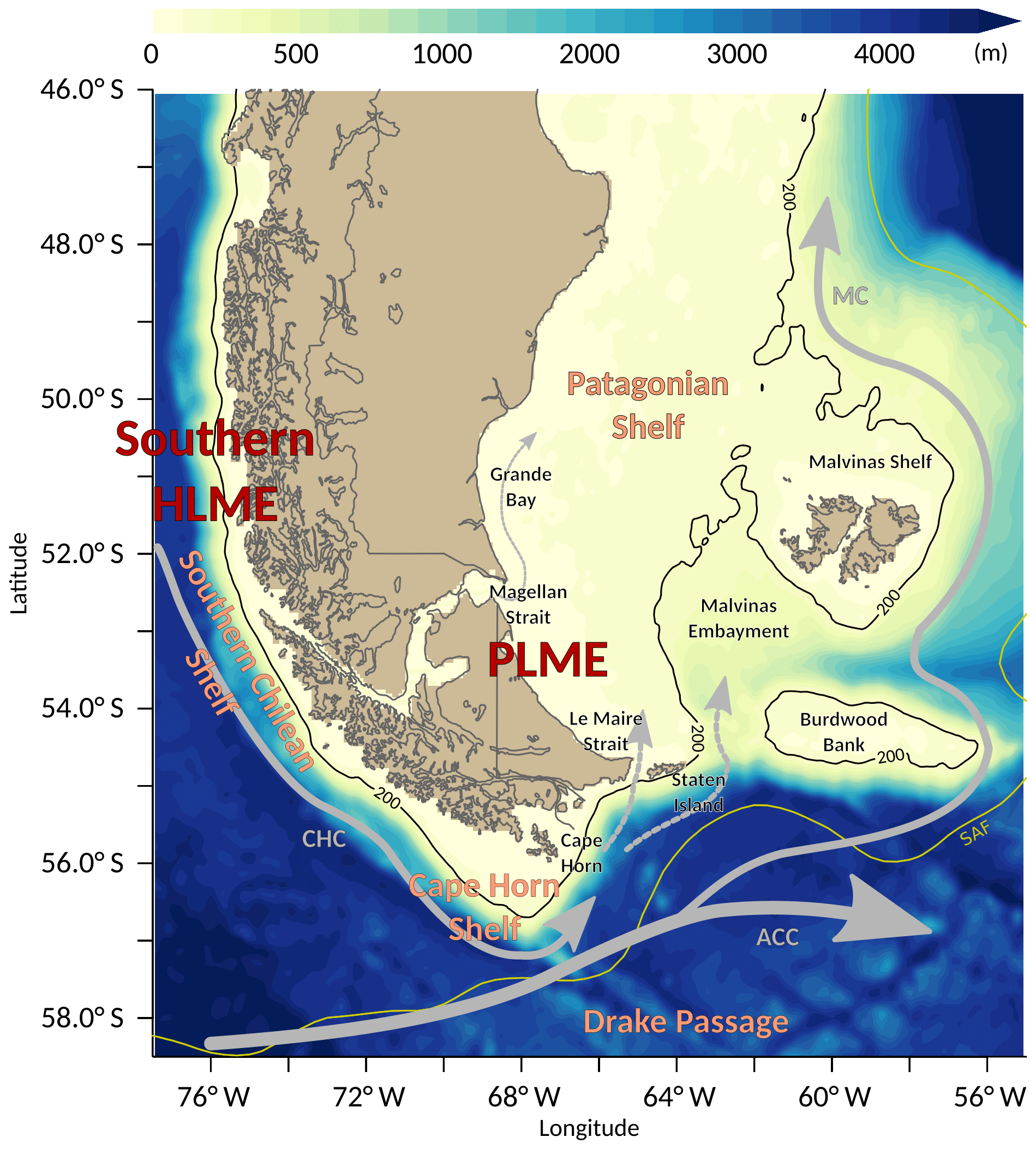
Figure 1 Domain of study and main geographic features. The colors show the bathymetry (m) of the CMM model used in this study. The northern branch of the Antarctic Circumpolar Current (ACC), the Cape Horn Current (CHC), and the Malvinas Current (MC) paths are shown in grey, and the southern Subantarctic Front (SAF), as defined by Kim and Orsi (2014), is shown in yellow.

The HLME is a prototypical eastern boundary upwelling system that extends from northern Peru to southern Chile in the South Pacific Ocean (see Heileman et al., 2009, for a detailed description), where it is adjacent to the PLME (Fig. 1). The HLME can be separated into two meridional subregions marked by the Subtropical Front at 35–40^∘ S (Chaigneau and Pizarro, 2005). About 65 % of the area of the HLME corresponds to the northern region and is under the influence of the Humboldt Current system and coastal upwelling from 4 to 40^∘ S. South of ≈45^∘ S the HLME is mostly under the influence of downwelling-favorable (poleward) winds and the poleward-flowing Cape Horn Current (CHC; Strub et al., 2007) along the shelf break of the southern Chilean Shelf (SCHS; 40–55^∘ S), a region with a complex fjord system. Further south, the shelf widens onto the Cape Horn shelf (CHS) region, marking the northern boundary of the Drake Passage.

At the southern tip of South America, the westerlies are strong, and schematic reconstructions of the annual mean ocean circulation in this area, based on hydrographic observations and models, show that the main flow patterns are from the Pacific towards the Atlantic (Combes and Matano, 2014a). The Antarctic Circumpolar Current (ACC) flows eastwards carrying cold and fresh (34 PSU) Subantarctic waters (Piola and Gordon, 1989; Peterson and Whitworth III, 1989) that are rich in nutrients (Acha et al., 2004; Romero et al., 2006) from the Drake Passage along the upper portions of the western slope of the Argentine basin. In the Drake Passage the northern boundary of the ACC is marked by a salinity minimum north of the Subantarctic Front (SAF) (Peterson and Whitworth III, 1989; Kim and Orsi, 2014) (Fig. 1).

The PLME is located in the southwestern Atlantic Ocean (see Heileman, 2009 for a detailed description) and embraces the Patagonian Shelf (hereafter PS), the largest continental shelf of the Southern Hemisphere (Bisbal, 1995), stretching from 37 to 55^∘ S and reaching up to 850 km off the coast in its widest portion (51^∘ S). The PS is characterized by low-salinity waters fresher than 33.8 PSU, with minor seasonal and vertical salinity variations (Piola et al., 2010); it is subjected to strong westerly winds and large-amplitude tides (e.g., Palma et al., 2004). An outstanding dynamical feature on the shelf is the Magellan Plume, derived from the discharge of relatively fresh waters through the Magellan Strait at 52.5^∘ S. This inflow explains the low salinity on the shelf and extends from 54 to 42^∘ S, which is up to 1800 km downstream (Piola et al., 2018, and references therein). The offshore boundary of the PS is marked by strong western boundary currents, the Brazil Current at the northern extremity flowing southwards, and the Malvinas Current (hereafter MC) south of about 38^∘ S, flowing northwards. The MC is derived from a deflection of the northern branch of the ACC around the PS. The thermohaline contrast between the MC and shelf waters creates a remarkable shelf-break front (e.g., Peterson and Whitworth III, 1989; Acha et al., 2004; Saraceno et al., 2004; Romero et al., 2006).

The southern section of the PS is the area where exchange with Pacific and Subantarctic waters takes place via the Magellan Strait, Le Maire Strait, and the shelf break. The Magellan Strait links the Pacific and Atlantic at 52^∘ S through a 570 km long channel of complex geomorphology with varying width, from a few kilometers at the Primera Angostura and Segunda Angostura narrows to more than 50 km near the eastern mouth. The Magellan Strait is very shallow on the eastern basin (<50 m) and exceeds 1000 m in the western basin. There is only one observationally based estimate of Pacific to Atlantic net throughflow via the Magellan Strait ranging between 0.04 and 0.07 Sv (Brun et al., 2019), while numerical models indicate a net flow towards the Atlantic of 0.085 Sv (Palma and Matano, 2012). The 30 km wide Le Maire Strait separates the southeastern tip of Tierra del Fuego from Staten Island (Isla de los Estados) at 54.83^∘ S. Situated downstream of Cape Horn, the Le Maire Strait is under the influence of strong currents flowing along the shelf break and the SAF (Orsi et al., 1995). Little is known about the transport and dynamics into the strait itself. On the eastern side of Staten Island, the shelf break turns abruptly north up to 51^∘ S where it diverges eastward towards the islands of the Malvinas Shelf. The Malvinas Embayment (ME) separates the PS from the shallower Burdwood Bank and the open ocean.

The lack of direct transport observations make it difficult to determine the variability of the exchange between the HLME and PLME. The complex morphology of the Patagonian area (rugged coastline, narrow straits, and enclosed bays) hampers the use of remote sensing such as satellite altimetry. Intrusions of high chlorophyll a on the PS via the Le Maire Strait have been observed (Romero et al., 2006), but the cloud coverage makes it difficult to use as time series. Surface drifters released in the Pacific usually end up ashore along the rugged southern Chilean Shelf or follow the large-scale circulation paths (along the ACC and MC) but rarely reach the PS, and Argo floats are not designed to work on shallow shelf areas. Hydrographic observations are too scarce to understand the time variability. The most notable published studies are surveys of the Magellan Strait by Panella et al. (1991) and the GEF Patagonia cruises, which took place on the PS in 2005 and 2006 (Charo and Piola, 2014). However, such in-depth studies have not been reconducted since and therefore cannot be used to evaluate the variability.

There have been a few modeling studies on the circulation of the PS evaluating its interactions with the deep ocean (e.g., Combes and Matano, 2018). However, no studies have focused on the exchange between the SCHS and the southern PS or on their property exchanges with the deep ocean and their drivers. Here, using 27 years (1980–2006) of numerical simulations at 1∕12^∘, we aim to quantify the exchange between the LMEs and establish a budget of the volume transport around the southern tip of South America. The flows through the straits and shelf–open-ocean exchanges contributing to the variability of the transport and its link with climate indices are discussed. The paper is organized as follows: Sect. 2 presents the datasets used in this study, Sect. 3 presents the mean simulated transport in the region and assesses the exchange between the LMEs, Sect. 4 focuses on the seasonal and interannual variability of these exchanges, and the results are summarized and discussed in Sect. 5.

2 Data

The model used in this work is the Regional Ocean Modeling System (ROMS; Shchepetkin and McWilliams, 2005) in a regional eddy-resolving configuration at 1∕12^∘. The model features a free surface, 40 σ levels with terrain-following coordinates on the vertical (Shchepetkin and McWilliams, 2005), and two-way nesting in a parent grid of 1∕4^∘ of the Southern Hemisphere, allowing for the forcing of the deep-ocean circulation at the boundaries. The spin-up spans 15 years: 10 years for the parent model and 5 additional years for the parent–child configuration, followed by a 34-year integration (1979–2012). This model configuration has previously been described by Combes and Matano (2014a) and widely used for studies on the Patagonian Shelf (e.g., Combes and Matano, 2014b, 2018). CMM is forced at the surface by monthly ERA-Interim winds (Dee et al., 2011) and heat and freshwater fluxes from the Comprehensive Ocean–Atmosphere Data Set (COADS) (Da Silva and Young, 1994), with a tendency-restoring term to the Pathfinder SST climatology. The eight main tidal components are also included. The bathymetry is smoothed from ETOPO1 (Amante and Eakins, 2009) to minimize the pressure gradient errors associated with terrain-following coordinates (Mellor et al., 1994). The Magellan Strait is resolved as a channel with a constant depth of 100 m and a fixed salinity of 31 at the Atlantic mouth to simulate the effect of freshwater input from rivers and glaciers. For more specific details about the configuration, the reader is referred to Combes and Matano (2014a). The configuration domain extends from 81 to 52.5^∘ W in longitude and 60 to 40^∘ S in latitude (reduced around the region of study in Fig. 1 to improve legibility). A total of 27 years (1980–2006) of monthly fields are used in this work, and thus all sub-monthly and high-frequency processes such as tides and the synoptic atmospheric variability are filtered out.

In addition to the above-described simulation, the ORCA0083-N06 simulations based on the NEMO code (Madec, 2014), developed by the Marine System Modelling team at the National Oceanography Centre (NOC), are used for comparison purposes. ORCA0083-N06 (hereafter referred to as ORCA) is a 1∕12^∘ global configuration available monthly over 33 years (1978–2010). ORCA is a global configuration featuring 75 vertical z levels with a grid spacing ranging from 1 m near the surface to 200 m at the bottom, with partial steps. ORCA features a nonlinear free surface. The bathymetry is derived from ETOPO2 (https://www.ngdc.noaa.gov/mgg/global/etopo2.html, last access: 28 January 2020; NGDC, 2006). ORCA uses a turbulent kinetic energy (TKE) mixing scheme (Blanke and Delecluse, 1993) and a total variance dissipation (TVD) advection scheme for active tracers (Madec, 2014). It is forced at the surface by the DRAKKAR forcing set atmospheric reanalysis (Brodeau et al., 2010), composed of ERA40 reanalysis winds and fluxes from the CORE2 reanalysis. ORCA does not include tides. It has successfully been used for Arctic (e.g., Kelly et al., 2018) and Southern Ocean (Mathiot et al., 2011; Duchez et al., 2014) studies.

Lagrangian analyses are conducted using the Ariane software (Blanke and Reynaud, 1997). This open-source tool available at http://www.univ-brest.fr/lpo/ariane (last access: September 2019) computes offline 3-D streamlines from the simulated velocity field from an ocean general circulation model (OGCM) such as NEMO or ROMS. It computes the time of advection between two cells, avoiding interpolation problems. There is no stranding parameterized. In this study Ariane is used in forward and backward modes applied to the 27 years of outputs from the ROMS configuration.

3 Exchange between the two LMEs

3.1 Mean transport and circulation

The PLME and HLME are subjected to various dynamical patterns. On the HLME, the narrow SCHS (extending from 0 to 100 km in width) that stretches from 48 to 53^∘ S features a complex coastline and the western mouth of the Magellan Strait. It differs greatly from the CHS at the tip of South America, where the continental slope orientation changes abruptly and the shelf is wider. In the Atlantic, the PLME can be separated into three subregions featuring different dynamics and/or topography. First, the southern Patagonian Shelf (SPS), extending from the southern tip of Tierra del Fuego to 47^∘ S, can itself be subdivided into two regions. SPS1, from the Le Maire Strait to Grande Bay at 51^∘ S, presents the more complex topography and is the region where exchange with the Pacific waters takes place through the Magellan Strait, Le Maire Strait, and the shelf break. SPS2, located further north, extends from 49.5 to 47^∘ S. Further east, the transports are evaluated in the Malvinas Shelf (MIS) region. The southern MIS is protected from a direct influence of the ACC by the shallower Burdwood Bank. Only a branch of this strong current, deflected between the PS and Burdwood Bank, enters the Malvinas Embayment and flows along the southern slope before joining the northward-flowing MC further north.

A volume transport budget of each of the above-described areas is calculated over the period as a mean over 27 years of the monthly velocities from CMM, vertically integrated down to 200 m deep. The transport is estimated normal to the 200 m isobath across the shelf break and is defined as positive poleward in the Pacific, equatorward in the Atlantic, and towards the shelf in the whole region. In the Malvinas Embayment area, which is not a shelf section, the transport is calculated in the upper 200 m layer and defined positive in the direction of the mean flow, which is towards the north in the southern section and towards the east in the eastern section. Each region has a closed budget (T_net≈0). Figure 2 shows the mean circulation in each of the previously defined areas. Black arrows schematically show the direction and intensity of the transport across the various sections.

Figure 2 Mean total schematic transport over 27 years in the upper layer (0–200 m) calculated from CMM on the southern Chilean Shelf (SCHS), Cape Horn shelf (CHS), southern Patagonian Shelf (SPS1 and SPS2), the Malvinas Shelf (MIS), and the Malvinas Embayment. The color bar represents the mean surface salinity from the model, and vectors represent the full mean depth-averaged velocity (surface to bottom). Black arrows and values indicate the integrated transport across each section.

On the Pacific shelf (SCHS), the current is poleward and then veers around the CHS, with an inflow from the shelf break. The eastward transport at the Cape Horn section (68^∘ W) reaches 0.95 Sv, flowing in eastward on the northern continental shelf of the Drake Passage. On the PS, the mean flow is positive (equatorward) and presents a total along-shelf transport of 1.33 Sv at 47^∘ S.

In the SPS1 region, there is a net inflow from the Magellan Strait (0.10 Sv), Le Maire Strait (0.17 Sv), and the shelf break (0.62 Sv). These inflows are compensated for by a net northward outflow of 0.88 Sv at 51^∘ S. This mass balance is in line with previous studies (0.5 to 0.8 Sv, based on a regional implementation of the Princeton Ocean Model; Palma et al., 2008; Matano and Palma, 2008). The transport through both straits accounts for 30 % of the total inflow onto the SPS, with a larger inflow through the Le Maire Strait than the Magellan Strait. The main source of waters to the SPS is through the shelf break (0.62 Sv) and is associated with the inflow of waters across the southern Malvinas Embayment section. Most of this on-shelf transport (0.5 Sv) occurs south of 52.5^∘ S. Though the transport through the Magellan Strait is minor, it greatly impacts the hydrographic characteristics of the PS, generating a coastal jet that leads to the development of a low-salinity plume extending downstream up to 46^∘ S. The MIS is more exposed to the influence of open-ocean waters and the MC. A net inflow of 1.15 Sv penetrates through the southern section (mainly from the Malvinas Embayment, accounting for 70 % of the total inflow), and 0.52 Sv exits northward towards the MC. A large fraction of the intruding waters (0.64 Sv) remains on the shelf and flows westwards to join the net equatorward flow on the PS. Both flows, from SPS1 and MIS, join and flow into SPS2. This is the only location where we observe a significant off-shelf (negative) transport (−0.28 Sv) from the PS, even if most of the water (80 %) entering the SPS2 through its southern boundary remains on the shelf and flows equatorwards.

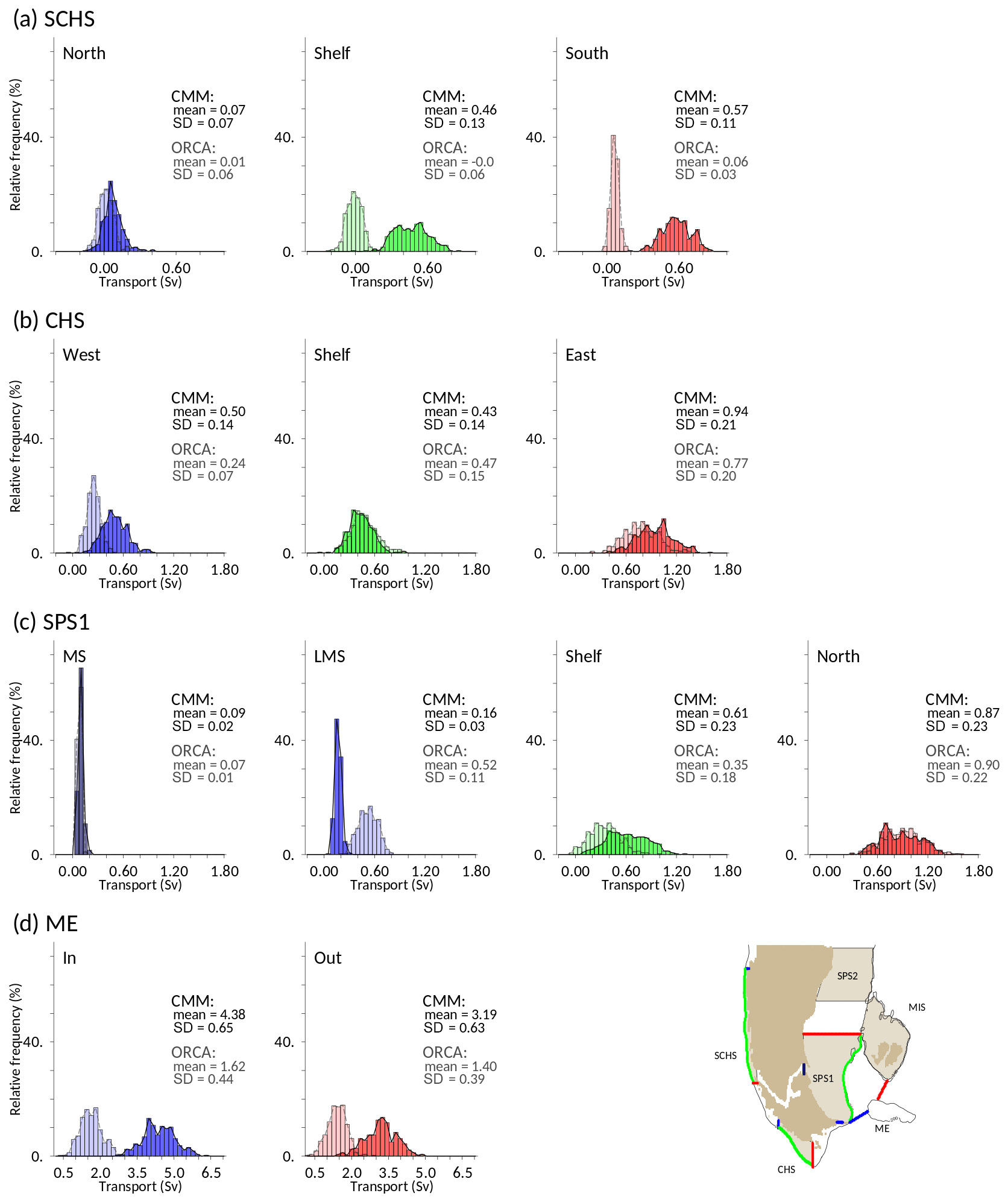
Figure 3 Histogram of transport over the 27 years at key locations of the SCHS (a), the CHS (b), the SPS1 (c), and the Malvinas Embayment (d), calculated along the colored sections indicated in the reference map. Opaque bins are from CMM, and transparent bins are from ORCA. The mean and standard deviation are indicated for each section. The transport is calculated over 200 m for all sections except for the Malvinas Embayment sections, where it is computed throughout the water column.

The above-described transports are based on the numerical results from CMM. For comparison we have also analyzed the ORCA outputs over the same subregions. Figure 3 displays the probability distribution of the monthly transport values for both models (here the transport in the Malvinas Embayment is calculated over the whole water column). The distributions are close to Gaussian, the exception being very narrow pathways like the SCHS, the northwestern limit of the CHS, the Magellan Strait, and the Le Maire Strait, especially in ORCA. The main differences between model results are concentrated on the southern sector of the SCHS where ORCA shows lower mean values in cross-shelf and along-shelf transports and decreased temporal variability. Additionally, and in contrast with the CMM results, the main source of waters to SPS1 in ORCA is the Le Maire Strait (0.52 Sv), whereas only 0.35 Sv enters via the shelf break. In wider sectors like the CHS, SPS1, and SPS2 (not shown), the agreement is better for both the mean and the variability.

3.2 Fate and origin of the LME waters

Two sets of Lagrangian experiments using Ariane were conducted to investigate the fate of HLME and PLME waters.

The first set was intended to explore the impact of the mean flow and employs the CMM climatological velocity fields. Initially, particles were released on all shelf grid points onshore from the 200 m isobath (see the green areas in Figs. 4a, 5a, and 6a) at the surface, at 50 m, and at 100 m, then advected by the mean flow during 90 d. It is important to note that though particles are released at a specific depth, they are free to displace vertically with the currents. Figures 4, 5, and 6 show the initial and final positions of the particles released at the surface, at 50 m, and at 100 m (panels a–c), as well as the trajectories, colored by depth (panels d–f). In order to render visibility in the figures, only 1 out of every 20 trajectories is represented.

On the SCHS, the particles are released from 47^∘ S along the Chilean coast up to Cape Horn at 68.3^∘ W (Fig. 4). The experiment represents a population of 1534 particles at the surface and 700 particles at 100 m of depth. The similarity of trajectories at the three depths suggests that particles travel at similar velocities despite the different release depths. While a few particles enter the Magellan Strait and flow directly towards the Atlantic, the majority take a poleward path to Cape Horn. The particles closest to the slope sink and join the CHC at depths greater than 150 m. Upon reaching Cape Horn, the particles that remain shallower than 100 m (light blue and yellow trajectories in Fig. 4d–f) follow the shelf break and either intrude into the PS via the Le Maire Strait or flow into the Malvinas Embayment through the passage between Staten Island and Burdwood Bank. The particles deeper than 100 m either follow a path along the SAF, around the southern slope of Burdwood Bank, or enter the Malvinas Embayment along a path similar as the surface particles.

Figure 4 Forward Lagrangian advection of particles during 90 d released on the SCHS. Initial positions (green) and final positions (red) of particles released at 0 m (a), 50 m (b), and 100 m (c). Vectors show the velocity at each depth. Particle trajectories colored by depth (m) for initial release at 0 m (d), 50 m (e), and 100 m (f) (1 out of 20 trajectories shown). The number of particles (n) for each experiment is shown, and the SAF is indicated in black.

A similar experiment is carried out by releasing particles on the PS (Fig. 5). In this region, distinct trajectories are observed between the surface and subsurface layers. Most of the surface particles are rapidly advected towards the shelf break, where they join the MC. When the MC reaches the confluence zone at ≈40^∘ S, they retroflect and flow southwards towards the open ocean (Fig. 5a). All the surface particles remain at the surface. At 50 and 100 m of depth, the particles drift onshore at relatively weak velocities. After 3 months of advection, most of the particles remain on the shelf. The particles close to the eastern mouth of the Magellan Strait are advected upwards as they approach the inner shelf (Fig. 5b). This onshore flow and subsequent upwelling compensates for the eastward advection of the surface layer. Thus, the cross-shore circulation is consistent with Ekman dynamics under intense westerly winds, which drive the surface waters northeastward and induce onshore flow in deeper layers and upwelling closer to the coast. In the central and eastern part of the shelf, the particles flow northward along the shelf. Though several particles reach the shelf break very few are exported to the MC. These particles flow along the shelf break, and some are upwelled around 46^∘ S.

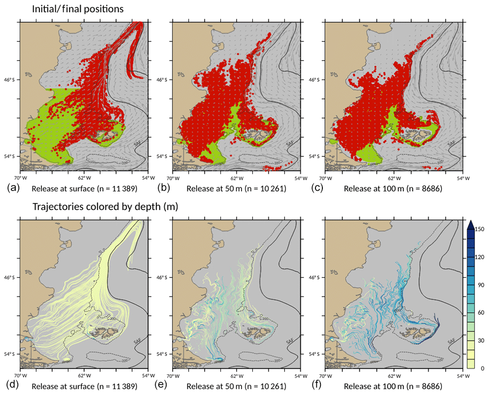
Figure 5 Forward Lagrangian advection of particles during 90 d released on the PS. Initial positions (green) and final positions (red) of particles released at 0 m (a), 50 m (b), and 100 m (c). Vectors show the velocity at each depth. Particle trajectories colored by depth (m) for initial release at 0 m (d), 50 m (e), and 100 m (f) (1 out of 20 trajectories shown). The number of particles (n) for each experiment is shown, and the SAF is indicated in black.

While these forward Lagrangian experiments confirm the flow of Pacific shelf waters into the PS and the equatorward flow in the Atlantic basin, they do not provide information about the possible inflow of open-ocean waters onto the shelf. To this end, we implemented an experiment prescribing a backward integration of 150 d from particles that reached SPS1 (Fig. 6). This experiment shows that the majority of surface waters in the PS originate in the Cape Horn shelf and enter the Atlantic through the Magellan and Le Maire straits and east of Staten Island. These particles are either derived from the surface waters in the southeast Pacific, north of 56^∘ S at 76^∘ W, or from the CHC. The deeper particles come from further north along the slope current (meaning they traveled faster), and several of these particles flow along the shelf break north of the SAF before reaching the CHS. It is important to note that apart from a few particles on the Malvinas Shelf, there are no waters originally deeper than 100 m entering the shelf in this climatological experiment, and there are no waters derived from south of the SAF reaching the Atlantic shelf.

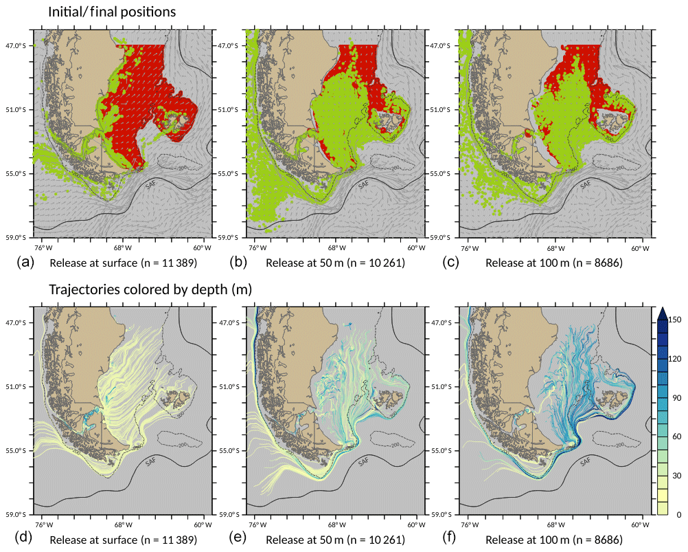
Figure 6 Backward Lagrangian advection of particles during 150 d that reached the PS. Initial positions (green) and final positions (red) of particles released at 0 m (a), 50 m (b), and 100 m (c). Vectors show the velocity at each depth. Particle trajectories colored by depth (m) for initial release at 0 m (d), 50 m (e), and 100 m (f) (1 out of 20 trajectories shown). The number of particles (n) for each experiment is shown, and the SAF is indicated in black.

The above-described particle paths indicate that the Drake Passage and CHS represent a key region for exchange between the two LMEs, as no particle released south of 57^∘ S in the averaged fields penetrates the PS. At the latitude of Cape Horn, the shelf features a change in orientation and is under the influence of strong flows associated with the SAF and the northern branch of the ACC.

The second group of Lagrangian experiments employed monthly averaged currents from CMM and monthly releases to better quantify the effect of mesoscale and long-term variability on the pathway of particles flowing through the northern Drake Passage. Particles are released on all grid points from 0 to 200 m at 68.1^∘ W (Cape Horn), from the coast (at 55.7^∘ S) to 58.5^∘ S, and advected during 1 year by the monthly averaged currents and density fields from CMM. This simulation is repeated monthly from 1980 to 2005, which makes 324 simulations of 365 d each. This corresponds to a release of 1649 particles per run (818 on CHS, which is from 55.7 to 56.67^∘ S, and the rest to the open ocean). At the end of each simulation, the particles that have reached SPS1 or the Malvinas Embayment are selected. The particles reaching the Malvinas Embayment through SPS1 are not counted twice and are consequently only considered to be particles reaching SPS1. These specific particles are then run backwards from their initial location (along Cape Horn) during 30 d to identify their origin. This experiment is designed to highlight the trajectory of the particles through the northern Drake Passage and CHS, from the Pacific to the PS, and properly assess their preferred path. Figure 7 displays the cumulative density of particles (summed from all the simulations) flowing through the Drake Passage and reaching SPS1 (Fig. 7a) and the Malvinas Embayment (Fig. 7c) after 90 d of advection. Figure 7 shows the propagation of the particles onto SPS1 (Fig. 7b) and the Malvinas Embayment (Fig. 7d) at 30, 90, 180, and 365 d.

On average for each simulation, 509 particles reach SPS1, and 381 reach the Malvinas Embayment. Among them, 93 % of the particles flowing through SPS1 and 49 % of the particles flowing through the Malvinas Embayment come from the CHS. No particle south of 57.48^∘ S reaches SPS1. The density distribution shows that a large number of particles enters SPS1 through the Le Maire Strait (Fig. 7a, b). These particles are advected all along the eastern side of the PS in 90 d, but they take longer to cover the coastal part of the shelf. After 1 year of advection, the particles have covered the entire SPS. The easternmost particles eventually flow south of the islands of the Malvinas Shelf and join the MC. The particles flowing directly through the Malvinas Embayment (Fig. 7b, d) penetrate the MIS area rapidly (in 30 to 90 d) and enter SPS2 but do not reach the coastal zone during the time of these experiments. The majority of the flow joins the MC along the slope.

Figure 7 Pathways of the monthly release of particles at Cape Horn (68.1^∘ W, from 58.5^∘ S to the coast) on the 0–200 m layer. Arrival at the Atlantic section through (a, b) SPS1 and (c, d) the Malvinas Embayment. Simulations are run backward for 30 d and forward for up to 365 d. (a, c) Cumulative square-meter density (number of particles per square meter simulations of 90 d. The drifter trajectories towards each area are shown in green. The dotted line at 68.1^∘ W shows the release section, and the black area shows the SPS1 and Malvinas Embayment areas, respectively. (b, d) Color shading shows the propagation of the advected particles after 30, 90, 180, and 365 d from dark to light blue.

A similar experiment was carried out over the 200–1000 m layer (Fig. 8): of the 137 172 particles that were released in total, only 127 reached SPS1, which is less than 1 particle per simulation. Moreover, the mean initial depth of these particles was 220 m, and they were located very close to the shelf break (the most austral particle was initially at 56.94^∘ S). A relatively small number of particles reaches the Malvinas Embayment (≈17 particles per simulation). Some of these particles came from greater depths (up to 850 m) but were mostly located close to the shelf break (90 % of these particles were deployed north of 57^∘ S). This is consistent with the previous result that the majority of the waters occupying the PS are derived from the upper layer of the Pacific and that little to no water from south of the SAF enters the PS.

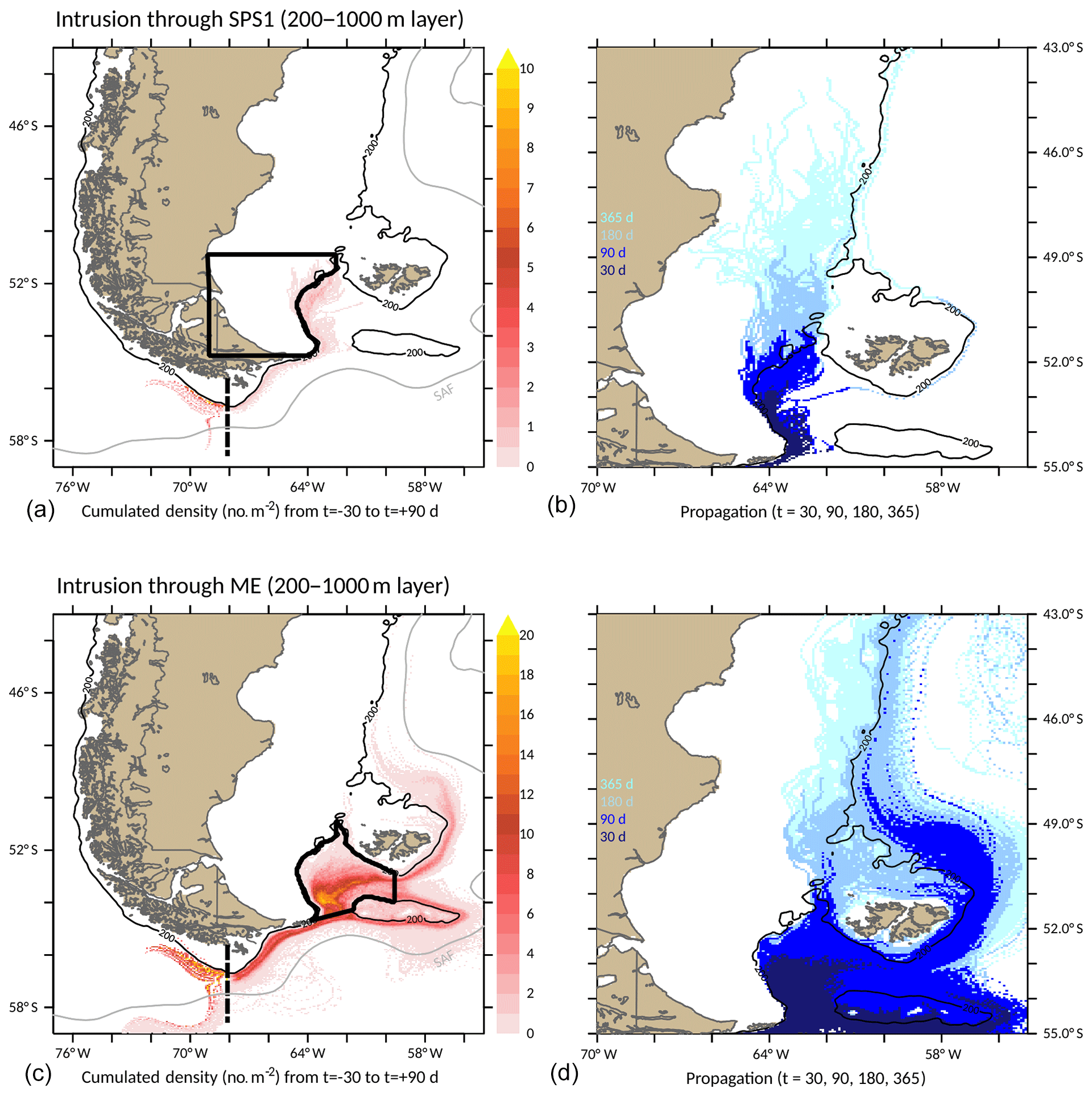
Figure 8 Pathways of the monthly release of particles at Cape Horn (68.1^∘ W, from 58.5^∘ S to the coast) on the 200–1000 m layer. Arrival at the Atlantic section through (a, b) SPS1 and (c, d) the Malvinas Embayment. Simulations are run backward for 30 d and forward for up to 365 d. (a, c) Cumulative square-meter density (number of particles per square meter), which is the cumulative spatial distribution after 324 simulations of 90 d. The dotted line at 68.1^∘ W shows the release section, and the black area shows the SPS1 and Malvinas Embayment areas, respectively. (b, d) Colors show the propagation of the advected particles after 30, 90, 180, and 365 d from dark to light blue.

Putman and He (2013) used HYCOM model outputs to explore temporal resolution effects on particle-tracking experiments in the North Atlantic. Comparison with real drifters released in the Gulf Stream system indicated that daily snapshots better represented the real trajectories, while 30 d averages tended to underpredict speeds (although not direction). Numerical experiments of particle dispersal also indicated a bias towards higher cross-shelf transport when using low-temporal-resolution model outputs. Overall, however, their results were very dependent on particle release location and the associated dynamical characteristics of the regional ocean circulation (i.e., releases in the South Atlantic Bight were scarcely affected by temporal resolution). In this regard, it is important to note that our geographical area differs from the one analyzed in Putman and He (2013). The SCHS is very narrow and located on an eastern boundary, while the PS is extremely wide, bounded by a very stable western boundary current, and forced by large tides (not included in HYCOM) and steady westerly winds. Altimetry analysis has shown that this is a region (particularly the shelf) of very low eddy variability (see, for example, Goni et al. (2011) and their Fig. 9 for the PS, and Meredith (2016) and his Fig. 2 for the entire region). The CMM maximum temporal resolution is a 10 d average. We carried out additional exploratory experiments comparing trajectories forced with 30 d (30D) averages and 10 d (10D) averages. Some indication of higher drifter velocities in 10D can be seen near the surface. The overall pattern of particle dispersal for 10D, however, is very similar to 30D both for SCHS and PS (not shown).

Surface drifter trajectories, extracted from the Coriolis database (http://www.coriolis.eu.org/, last access: 28 January 2020), were compared against the above-described simulated trajectories (green lines in Fig. 7). A total of 89 trajectories, flowing on the HLME–PLME or through the northern Drake Passage, were recorded between 1980 and 2017. Among them, 33 drifters flowed onto the HLME or the PLME shelf. However, most drifters either ended by washing ashore in the numerous fjords of southern Chile or were released directly in the PLME and are therefore not useful to portray the exchange between the two shelves. Only two drifters went through the Drake Passage and penetrated the PS briefly before reaching the Malvinas Embayment. Three additional drifters directly entered the Malvinas Embayment after flowing through the Drake Passage. Even though the observational dataset is small and precludes a quantitative statistical analysis, the observed and simulated trajectories are in good qualitative agreement as no drifters flowing through the Drake Passage south of the SAF entered the embayment. This supports our conclusion about the Pacific origin of the PS water masses.

Some of the drawbacks of poor sampling can be alleviated with multiple releases and long-term tracking (Putman and He, 2013). The release of particles every 30 d (not just a single day), the long-term span of our tracking experiments, and the ensemble average of the results (Figs. 7 and 8) ensure a more robust interpretation of particle dispersion between the HLME and the PLME. Therefore, although we expect some influence of high-frequency input on our preliminary particle-tracking results, the only way to properly assess and quantify this effect would be to perform a dedicated series of experiments, something that is beyond the scope of our study.

4 Variability of the exchange

This section assesses the seasonal to interannual variability of the transport through selected sections and investigates the origin of this variability.

4.1 Seasonal variability

On the southern HLME, the seasonal across-shelf transport onto the SCHS is lowest in June (green line of Fig. 9a), coinciding with a minimum in the zonal wind seasonal variability. At the same time, the increase in southward transport through the northern shelf section (blue line of Fig. 9a) results in a small change in the southward export across the southern boundary of SCHS (0.16 Sv; red line in Fig. 9a). A similar seasonal cycle is found across the shelf of CHS and at its eastern section (Fig. 9b) but presents a higher amplitude (≈0.35 Sv) with a peak in austral summer and a minimum in June.

While the seasonal cycles of wind and transport intensity are positively correlated on the SCHS and CHS, this is not the case on the PS, where the transport minimum is observed in austral spring (Fig. 9c–e) and the averaged wind on SPS1 presents a lower (and negative) correlation with the across-shelf transport at that location. While the transport through the Magellan and Le Maire straits presents lower variability, the transport across the northern boundary of SPS1 is highly correlated with the transport variability across the shelf-break section (r=0.95), with a minimum in October (0.75 Sv) and a maximum in summer (1 Sv). This can partly be explained by an increased offshore Ekman surface transport in late summer, which decreases the inflow from the shelf break. Combes and Matano (2018) argue that these seasonal variations are modulated by the ACC. They also indicate that variations in the shelf inflow (i.e., through the SPS1 shelf break) and the ACC transport are out of phase. Thus, an increase (decrease) in the latter produces a weakening (strengthening) of the former. The larger ACC transport during late winter augments its inertial tendency to flow eastward along the southern flank of the Burdwood Bank and therefore weakens the portion of the flow diverted into the Malvinas Embayment (Fetter and Matano, 2008). In summer a weaker ACC increases its interaction with the Malvinas Embayment, boosting inflow to SPS1.

The transport variability on the MIS is more complex. The incoming transport through the southern boundary (blue line in Fig. 9e) does not present a marked seasonal variability. However, the northward flow towards the MC increases in austral winter (red line in Fig. 9e), which is partially compensated for by a transport decrease towards the SPS (green line in Fig. 9e). The transport through the southern and northern boundaries of SPS2 (blue and red lines in Fig. 9d, respectively) has very similar seasonal cycles to those observed at the offshore boundaries of SPS1 and MIS (green lines in Fig. 9c and e, respectively). Since the transports through the Magellan and Le Maire straits are relatively small, the seasonal variability of the northward transport in the southern PS appears to be closely associated with the variability of the shelf–open-ocean exchanges.

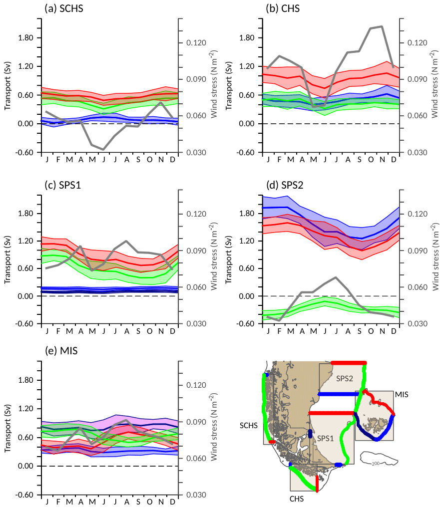
Figure 9 Mean seasonal variability of the transport across the key areas: SCHS (a), CHS (b), SPS1 (c), SPS2 (d), and MIS (e). The transport is defined as positive in the direction of the main flux (polewards in the Pacific, equatorwards in the Atlantic) and towards the shelf. The shaded areas represent the standard deviation from the 27 years of simulation. Bottom right shows a reference map of the sections of each key area where the seasonal transport has been calculated and their associated colors. The grey line in each panel is the zonal wind stress in the area, calculated in the shaded regions indicated in the reference map.

4.2 Interannual variability

Figure 10 shows the time series over 27 years of the transport anomaly along the borders of the key areas from the CMM simulations. Also shown in Fig. 10 are the spatially averaged zonal winds from ERA-Interim in the same areas, used as forcing for the simulations. A 12-month running mean is applied to the data to filter the seasonal signal. No significant trend in the transport is observed over the nearly 3 decades of simulations, nor is one observed in the forcing. The interannual variability of the transport anomalies in ORCA is in very good agreement with CMM (not shown), with a correlation above 0.7 on CHS and PS.

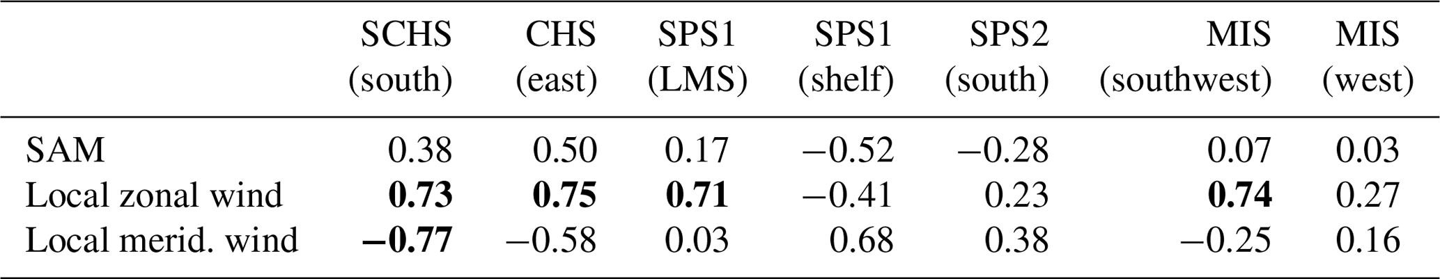
On the SCHS, the most significant anomaly occurs in 1998, when the inflow from the deep ocean decreased by ≈0.2 Sv, associated with a low zonal wind stress intensity. Further downstream, the southward inflow to the CHS from the shelf further north (blue line in Fig. 10b) is decorrelated from the exchange across the 200 m isobath, but the resulting eastward transport at 68^∘ W (red line in Fig. 10b) depends on both the along-shelf and across-shelf variability (correlations of 0.72 and 0.79, respectively). Both regions present an interannual variability correlated with the variability of the zonal and meridional components of the local wind (Table 2).

The variability of the transport anomaly on the southern PLME (SPS1 and SPS2) presents larger amplitudes than on the southern HLME, with remarkable minima in 1989 and 1999 and maxima in 1996 and 2003. The inflow through the Le Maire Strait, although small compared to the across-shelf exchange, is highly dependent on the upstream variations over the CHS (r=0.79, Table 1). The transport across the southwestern MIS section (cyan line in Fig. 10e) and the SPS shelf-break sections (green lines in Fig. 10c and d), though both are bounded by the Malvinas Embayment, are poorly correlated (r=0.14), suggesting that these exchanges are controlled by local dynamics. Indeed, the interannual anomaly of transport across the southwestern section of MIS if highly correlated with the interannual zonal wind averaged over the MIS area (r=0.74; Table 2). On the other hand, the intrusion of the MIS waters onto the PS through its western section is moderately correlated with the SPS1 transport anomalies (r=0.37), suggesting different drivers. The transport variations across the southern boundary of SPS2 (blue line in Fig. 10d) are equally dependent on the variability of the northern boundary of SPS1 (red line in Fig. 10e) and the western boundary in MIS (r=0.82 and 0.81, respectively). Positive transport anomalies across the southern boundary of SPS2 are associated with increased outflow at the shelf break.

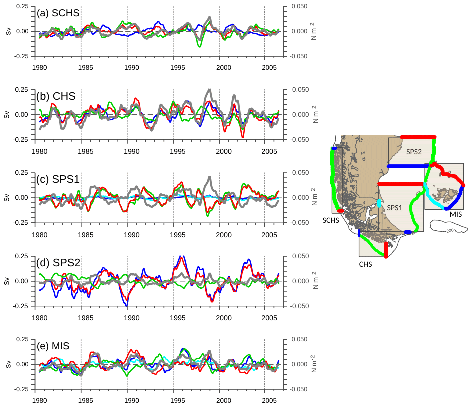
Figure 10 Monthly transport anomalies across the sections of the key areas. From top to bottom: SCHS (a), CHS (b), SPS1 (c), SPS2 (d), and MIS (e). On the right is a reference map that shows (in colors) the sections of each key area where the monthly transport has been calculated. The grey line in each panel is the zonal wind stress in the area, calculated in the shaded regions indicated in the reference map. A 12-month running mean is applied to the data to filter the seasonal signal.

Table 1 Correlation between interannual transport anomalies from CMM across selected sections: SCHS (south), CHS (east), SPS1 (LMS and shelf), SPS2 (south), and MIS (southwest and west). High correlations (equal to or above 0.7) are shown in bold.

Table 2 Correlation between the SAM, local wind anomalies, and the transport anomalies across selected sections calculated from CMM: SCHS (south), CHS (east), SPS1 (LMS and shelf), SPS2 (south), and MIS (southwest and west). For each section, the local wind anomaly is calculated in the shaded regions indicated in Fig. 10. High correlations (equal to or above 0.7) are shown in bold.

The analysis of the spatiotemporal variability of the simulated transport suggests that the interannual transport variability at the shelf-break boundary in SPS1 (green line in Fig. 10c) controls a substantial part of the variability of the northward transport all along the PS shelf. To further understand the nature of the interannual transport variability on the PS we compare the transport anomalies entering the SPS1 from the shelf break against climatic indices for both simulations. The transport variations show a significant correlation with the Southern Annular Mode (SAM) index (Marshall, 2003) in both CMM and ORCA ($r=-\mathrm{0.52}$ and −0.63, respectively; Fig. 11)

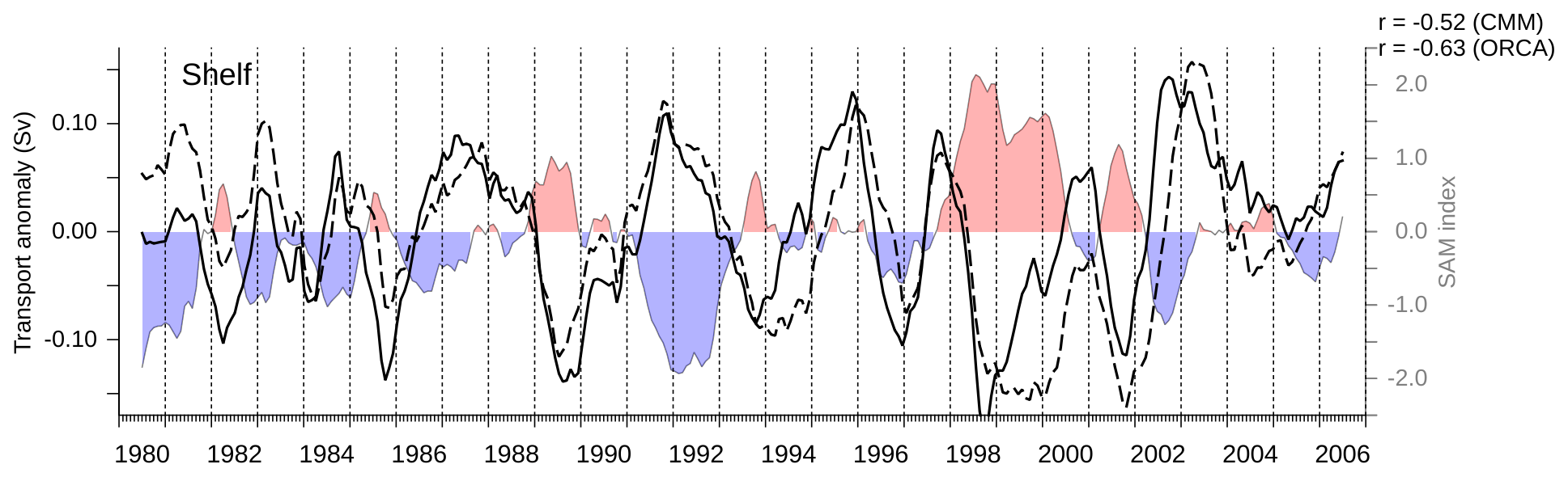
Figure 11 Monthly transport anomaly through the SPS1 shelf-break sections from CMM (solid line) and ORCA (dashed line), as well as the SAM index (positive and negative phases in red and blue, respectively). Correlations (r) between simulations and the SAM index are shown on the upper right-hand side. A 12-month running mean is applied to the data to filter the seasonal signal.

To further investigate the relationship between the SAM and the shelf transport we carried out an empirical orthogonal function (EOF) analysis of the zonal and meridional winds based on ERA-Interim data between 1980 and 2006. Though the mean zonal wind is significantly larger than the meridional wind, the amplitude of the interannual variability of both components is similar (Fig. S1 in the Supplement). The first EOF mode of the meridional wind (EOF1v), which explains 30 % of the total variability, presents a dipole structure with positive loadings over most of the southern portion of the shelf around southern South America and negative loadings farther north in the Pacific and farther northeast in the Atlantic (Fig. 12c). This spatial pattern is robust and also emerges in the first EOF modes of sea level pressure and meridional wind in the Southern Hemisphere south of 20^∘ S (see Fig. S2). The time series of EOF1v presents substantial interannual variability, which is significantly correlated with the SAM index (−0.67; Fig. 12e) and the northward transport through SPS1 (0.68; Fig. 12f). These results are in agreement with the recent analyses of Combes and Matano (2018), who suggested that the wind stress modulates the magnitude of cross-shelf exchanges at the southern boundary of the Atlantic shelf. As will be discussed below, the on-phase variations of the meridional winds at either side of South America have significant dynamical implications for the circulation over the continental shelves. The first EOF mode of the zonal wind (EOF1u), which explains 38 % of the total variability, shows a spatial structure very similar to EOF1v over southern South America, with a positive zonal band that reaches 40^∘ S (Fig. 12a). Its time series is also moderately correlated with the SPS1 transport anomalies, but they are out of phase, so during positive SAM phases stronger westerly winds drive weaker northward shelf transport. Note that although stronger westerlies promote larger northward Ekman transport, they also generate larger (southward) geostrophic coastal currents (Palma et al., 2008) that are in phase with the shelf transport anomalies.

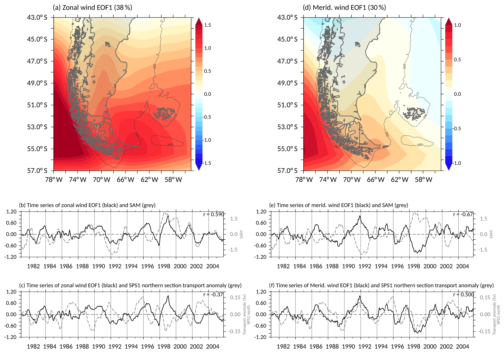
Figure 12 (a) Spatial pattern of the first EOF of zonal winds around southern South America. (b) Annual means of the first EOF mode of zonal wind (black) and the SAM index (grey), as well as (c) annual means of the first EOF of zonal wind (black) and northward transport through the northern boundary of SPS1 (grey). Panel (d) is the same as (a) but for the meridional wind. Panel (e) is the same as (b) but for the first EOF mode of the meridional wind. Panel (f) is the same as (c) but for the first EOF mode of the meridional wind. A 12-month running mean is applied to the data.

5 Conclusions

Our analyses of numerical simulations allow for the study of the exchange between the southern portions of the HLME and PLME and their variability over 3 decades. Results from two numerical models are used to quantify the transport over the shelf. Both simulations have been validated based on observations and have been widely used (Combes and Matano, 2018; Duchez et al., 2014). We used model outputs featuring the same space and time resolutions (monthly outputs at 1∕12^∘). However, the models were independently developed and feature different parameterizations. Though our objective is not to make a formal intercomparison of the models, due to the scarcity of observations, a discussion of their similarities and differences is useful to qualitatively determine which features of the circulation and their variability are more robust. While ORCA is a global configuration based on the NEMO code, the CMM configuration is a two-way nested simulation embedded in a 1∕4^∘ parent grid. Thus, elements of the large-scale circulation, such as the ACC, are resolved at 1∕12^∘ at a circumpolar scale in ORCA, whereas it is simulated at this resolution only in the child-grid domain in CMM. The choice of the vertical coordinate system (40 σ levels in CMM vs. 75 z levels in ORCA) plays an important role in the representation of the shelf and slope circulation. ORCA features only 31 levels in the upper 200 m. It is also important to note that the Magellan Strait inflow to the Atlantic shelf in the CMM simulation is implemented with a prescribed low salinity near the Atlantic mouth. In ORCA there is no correction on the Magellan Strait salinity, and therefore its discharge on the PS has salinities higher than observed. This point is of major importance in terms of water mass characteristics, but the resulting along-shelf transport is not significantly impacted by this correction, as the transport through the Magellan Strait is similar in both simulations and its contribution to the overall mass balance of the southern PS is relatively small. Despite all these differences, both models are in very good agreement in terms of circulation features over the shelf and present comparable transport intensities and variability, though ORCA presents less intense shelf–open-ocean exchange. For example, the transports across the shelf break from 51 to 54.8^∘ S (SPS1) in both models are well correlated (r=0.75). This transport is also highly correlated with the SAM index in both simulations, suggesting that the wind variability partially controls the exchange between the shelf and the adjacent deep ocean. It is also important to note at this point that both simulations are forced at the surface by ERA reanalysis (ERA-40 for ORCA and ERA-Interim for CMM). ERA-Interim features an improvement in resolution, data assimilation methods, and physics, but these changes do not greatly impact the representation of the winds at a monthly scale (Dee et al., 2011).

The combination of Lagrangian and time series analysis allows for a better understanding of the pathways and a quantification of the inputs of the different entry points into the southwest Atlantic shelf, as well as their variability. The shelf–deep-ocean transports were calculated across the 200 m isobath and not across strait sections, allowing for a fine evaluation of the shelf–sea exchange. The narrow SCHS is subject to open-ocean dynamics and the CHC, which flows along the shelf break. The PS waters originate from the SCHS and flow along the CHS. The majority of these waters enter the Atlantic shelf via the Le Maire Strait and the Malvinas Embayment shelf break. An additional contribution through the Magellan Strait, although smaller, is known to have a strong impact on the salinity and coastal circulation of the PS (Palma and Matano, 2012; Brun et al., 2019). The low-frequency variability of the shelf exchange in the SPS is partly explained by the large-scale wind variability, as determined by the SAM index.

The SAM modulates both wind components around southern South America. During positive SAM phases the zonal (meridional) component increases (decreases) and vice versa. The wind contribution on the shelf circulation, however, is known to be larger for along-shelf (i.e., meridional) winds than for cross-shelf (zonal) winds (Greenberg et al., 1997). Therefore, we hypothesize that the interannual variability of the along-shelf transport over this region is largely associated with the variability of the meridional component of the wind, which is negatively correlated with the SAM index. We argue that variations in the meridional component of the wind induce changes in the cross-shore Ekman transport and set up a cross-shore pressure gradient that in turn modulates the intensity of the along-shore currents over the Pacific and Atlantic shelves. Interestingly, the first EOF mode of the meridional winds is uniform over the southern tip of South America, implying that wind anomalies are in phase on the Atlantic and Pacific shelves. During negative SAM index periods southerly winds prevail on both shelves, implying upwelling winds on the Pacific and downwelling winds on the Atlantic. Thus, according to the proposed mechanism, the associated along-shelf geostrophic transport anomalies in the southeast Pacific shelf must be 180^∘ out of phase with the anomalies in the southwest Atlantic shelf (recall that positive transport is southward in the Pacific shelf and northward in the Atlantic shelf). Such an out-of-phase relationship is readily apparent when comparing the variability of the southward flow anomalies through the southern boundary of SCHS (black line in Fig. 13a) and the transport anomalies through the shelf break of SPS1 ($r=-\mathrm{0.52}$; grey line in Fig. 13a). Moreover, since the on-phase variability of the meridional wind over the Pacific and Atlantic shelves implies out-of-phase variations in coastal sea level, there must be a direct impact on the barotropic pressure gradient between the Pacific and Atlantic mouths of the Magellan Strait and hence on the associated transport. During positive SAM and negative (northerly) wind periods coastal sea level will rise in the Pacific and drop in the Atlantic, leading to increased transport from the Pacific to the Atlantic through the Magellan Strait. Such a relationship is also evident in the strong correlation between the transport through the Atlantic mouth of the Magellan Strait and the southward transport through the southern boundary of SCHS (r=0.77; Fig. 13b). These results are consistent with the sensitivity analysis carried out on realistic simulations of the Magellan Strait throughflow, which suggest a strong relationship between the inter-ocean sea level difference and the Magellan Strait transport (Sassi and Palma, 2006). Given that the Magellan Strait throughflow is the source of the lowest-salinity waters to the Atlantic shelf (Brun et al., 2019), periods of positive (negative) SAM, associated with enhanced (decreased) Magellan transport and decreased (enhanced) northeastward transport over the SPS, should lead to low-salinity (high-salinity) anomalies in this region. The SAM presents a positive long-term trend in response to the increase in anthropogenic forcing (Marshall et al., 2006). Should this positive SAM trend persist in the future it would lead to significant changes in the water mass characteristics (lower salinity) of the southern PS.

Figure 13 (a) Annual mean transport anomalies through the southern boundary of SCHS (black) and northward transport through SPS1 (grey). (b) Annual mean transport anomalies through the southern boundary of SCHS (black) and Pacific to Atlantic transport through the Atlantic mouth of the Magellan Strait (grey). The transports in (b) have been normalized with the maximum of each time series to help visualize the variability of the Magellan throughflow. The correlation between the transport anomalies is indicated on the right side of each panel. A 12-month running mean is applied to the data to filter the seasonal signal.

The analysis of 27 years of numerical simulations provided a regional understanding of the long-term exchange between two large marine ecosystems and allow for an assessment of the variability of this exchange. Further studies at increased spatiotemporal resolution are clearly needed at some key locations that are under-resolved or absent in CMM and ORCA. In particular, efforts must be made to provide a better representation of the narrowest geomorphological features such as the western sector and the Primera and Segunda Angostura narrows of the Magellan Strait, as well as the Beagle Channel, a very long and narrow passage (≈5 km) connecting the SCHS and the CHS to the south of Tierra del Fuego. This task would require the development of a new regional model at higher resolution, possibly nested to the 1∕12 models or employing unstructured grids. The model should incorporate continental discharge from glaciers and rivers as well as a better representation of the coastline and bottom topography. Daily outputs are required to improve the analysis of mesoscale variability and evaluate their impact on the exchanges described in this study. The combination of such higher spatiotemporal simulations with the current simulations would provide a finer picture of the exchange and allow for the quantification of the input from both the small-scale and large-scale circulation. Moreover, such modeling effort should be carried out in conjunction with observations at key locations of the Magellan Strait, Le Maire Strait, Beagle Channel, Cape Horn shelf, and the Malvinas Embayment, which would greatly improve our understanding of the water mass pathways in this complex region.

Despite the significant morphological and dynamical differences between the southern Humboldt Current and Patagonia LMEs, a number of biogeographical studies based on a variety of species and different methodology have suggested that south of 43^∘ S both regions share similar biological and environmental characteristics and belong to the Magellanic Province (Boschi, 2000; Sullivan Sealey, 1999; Spalding et al., 2007, and references therein). However, the causes of this relatively strong ecological connectivity are unknown. Our results suggest that the connectivity is mediated by a well-defined flux from the Pacific to the Atlantic, which may facilitate the dispersion of holoplanktonic species and planktonic larvae of benthic species, as well as fish larvae, towards the Atlantic.