Variability and stability of anthropogenic CO₂ in Antarctic Bottom Water observed in the Indian sector of the Southern Ocean, 1978–2018

Antarctic Bottom Water (AABW) is known as a long-term sink for anthropogenic CO₂ (C_ant), but the sink is hardly quantified because of the scarcity of observations, specifically at an interannual scale. We present in this paper an original dataset combining 40 years of carbonate system observations in the Indian sector of the Southern Ocean (Enderby Basin) to evaluate and interpret the interannual variability of C_ant in the AABW. This investigation is based on regular observations collected at the same location (63^∘ E–56.5^∘ S) in the framework of the French observatory OISO from 1998 to 2018 extended by GEOSECS and INDIGO observations (1978, 1985 and 1987).

At this location the main sources of AABW sampled is the low-salinity Cape Darnley Bottom Water (CDBW) and the Weddell Sea Deep Water (WSDW). Our calculations reveal that C_ant concentrations increased significantly in the AABW, from an average concentration of 7 µmol kg⁻¹ calculated for the period 1978–1987 to an average concentration of 13 µmol kg⁻¹ for the period 2010–2018. This is comparable to previous estimates in other Southern Ocean (SO) basins, with the exception of bottom water close to formation sites where C_ant concentrations are about twice as large. Our analysis shows that total carbon (C_T) and C_ant increasing rates in the AABW are about the same over the period 1978–2018, and we conclude that the long-term change in C_T is mainly due to the uptake of C_ant in the different formation regions. This is, however, modulated by significant interannual to multi-annual variability associated with variations in hydrographic (potential temperature, Θ; salinity, S) and biogeochemical (C_T; total alkalinity, A_T; dissolved oxygen, O₂) properties. A surprising result is the apparent stability of C_ant concentrations in recent years despite the increase in C_T and the gradual acceleration of atmospheric CO₂. The interannual variability at play in AABW needs to be carefully considered in the extrapolated estimation of C_ant sequestration based on sparse observations over several years.

1 Introduction

The carbon dioxide (CO₂) atmospheric concentration has been increasing since the start of industrialization (Keeling and Whorf, 2000). This increase leads to an ocean uptake of about a quarter of C_ant emissions (Le Quéré et al., 2018; Gruber et al., 2019a). It is widely acknowledged that the Southern Ocean (SO) is responsible for 40 % of the C_ant ocean sequestration (Matear, 2001; Orr et al., 2001; McNeil et al., 2003; Gruber et al., 2009; Khatiwala et al., 2009). Ocean C_ant uptake and sequestration have the benefit of limiting the atmospheric CO₂ increase but also result in a gradual decrease in the ocean pH (Gattuso and Hansson, 2011; Jiang et al., 2019). Understanding the oceanic C_ant sequestration and its variability is of major importance to predict future atmospheric CO₂ concentrations, the impact on the climate and the impact of the pH change on marine ecosystems (de Baar, 1992; Orr et al., 2005; Ridgwell and Zeebe, 2005).

C_ant in seawater cannot be measured directly, and the evaluation of the relatively small C_ant signal from total inorganic dissolved carbon (C_T; less than 3 %; Pardo et al, 2014) is still a challenge to overcome. Different approaches have been developed in the last 40 years to quantify C_ant concentrations in the oceans. The “historical” back-calculation method based on C_T measurements and preformed inorganic carbon estimates (C⁰) was independently published by Brewer (1978) and Chen and Millero (1979). This method has often been applied at the regional and basin scale (Chen, 1982; Poisson and Chen, 1987; Chen, 1993; Goyet et al., 1998; Körtzinger et al., 1998, 1999; Lo Monaco et al., 2005a). More recently, the TrOCA (Tracer combining Oxygen, dissolved Carbon and total Alkalinity) method has been developed (Touratier and Goyet, 2004a, b; Touratier et al., 2007) and applied in various regions including the SO (e.g., Lo Monaco et al., 2005b; Sandrini et al., 2007; Van Heuven et al., 2011; Pardo et al., 2014; Shadwick et al., 2014; Roden et al., 2016; Kerr et al., 2018). Comparisons with other data-based methods show significant differences in C_ant concentrations, especially at high latitudes and more particularly in deep and bottom water (Lo Monaco et al., 2005b; Vázquez-Rodríguez et al., 2009; Pardo et al., 2014).

Antarctic Bottom Water (AABW) is of specific interest for atmospheric CO₂ and heat regulation as it plays a major role in the meridional overturning circulation (Johnson et al., 2008; Marshall and Speer, 2012). AABW represents a large volume of water covering a major part of the world ocean floor (Mantyla and Reid, 1995), and its spreading in the interior ocean through circulation and water mixing is a key mechanism for the long-term sequestration of C_ant and climate regulation (Siegenthaler and Sarmiento, 1993). AABW formation is a specific process occurring in few locations around the Antarctic continent (Orsi et al., 1999). In short, AABW formation occurs when the Antarctic surface water flows down along the continental shelf. The Antarctic surface water density required for this process to happen is reached by the increase in salinity (S) due to brine release from ice formation and by a decrease in temperature due to heat loss to either the ice shelf or the atmosphere. Importantly, the AABW formation process is enhanced by katabatic winds that open areas free of ice called polynyas (Williams et al., 2007). Indeed, katabatic winds are responsible for an intense cooling that enhances the formation of ice constantly pushed away by the wind, leading to cold and salty surface water in contact with the atmosphere. The variable conditions of wind, ice production, surface water cooling and continental slope shape encountered around the Antarctic continent lead to different types of AABW, and hence the AABW characteristics can be used to identify formation sites.

The ability of AABW to accumulate C_ant has been controversial since one can believe that the ice coverage limits the invasion of C_ant in Antarctic surface water (e.g., Poisson and Chen, 1987). This is, however, not the case in polynyas, and several studies have reported significant C_ant signals in AABW formation regions, likely due to the uptake of CO₂ induced by high primary production (Sandrini et al., 2007; van Heuven et al., 2011, 2014; Shadwick et al., 2014; Roden et al., 2016). However, little is known about the variability and evolution of the CO₂ fluxes in AABW formation regions, and since biological and physical processes are strongly impacted by seasonal and interannual climatic variations (Fukamachi et al., 2000; Gordon et al., 2010; McKee et al., 2011; Gordon et al., 2015; Gruber et al., 2019b), the amount of C_ant stored in the AABW may be very variable, which could bias the estimates of C_ant trends derived from datasets collected several years apart (e.g., Williams et al., 2015; Pardo et al., 2017; Murata et al., 2019).

In this context of potentially high variability in C_ant uptake at AABW formation sites, as well as in AABW export, circulation and mixing, we used repeated observations collected in the Indian sector of the Southern Ocean to explore the variability in C_ant and C_T in the AABW and evaluate their evolution over the last 40 years.

2 Study area

2.1 AABW circulation in the Atlantic and Indian sectors of the Southern Ocean

The circulation in the SO is dominated by the Antarctic Circumpolar Current (ACC) that flows eastward, while the Coastal Antarctic Current (CAC) flows westward (Carter et al., 2008). The ACC and the CAC influence the circulation of the entire water column and generate gyres, which are crucial drivers of SO circulation (Carter et al., 2008). The most important gyres encountered around the Antarctic continent correspond to major AABW formation sites (Fig. 1). The main AABW formation sites are the Weddell Sea, where Weddell Sea Deep Water and Weddell Sea Bottom Water are produced (WSDW and WSBW, respectively; Gordon, 2001; Gordon et al., 2010), the Ross Sea for the Ross Sea Bottom Water (RSBW; Gordon et al., 2009, 2015), the Adélie Land coast for the Adélie Land Bottom Water (ALBW; Williams et al., 2008, 2010) and the Cape Darnley Polynya for the Cape Darnley Bottom Water (CDBW; Ohshima et al., 2013). AABW formation has also been observed in the Prydz Bay (Yabuki et al., 2006; Rodehacke et al., 2007). There, three polynyas and two ice shelves have been identified as Prydz Bay Bottom Water (PBBW) production hotspots from seal tagging and mooring data (Williams et al., 2016). This PBBW flows out of the Prydz Bay through the Prydz Channel and gets mixed with the CDBW. The mix of CDBW and PBBW (hereafter called CDBW) represents significant AABW export (13 % of all AABW export; Ohshima et al., 2013).

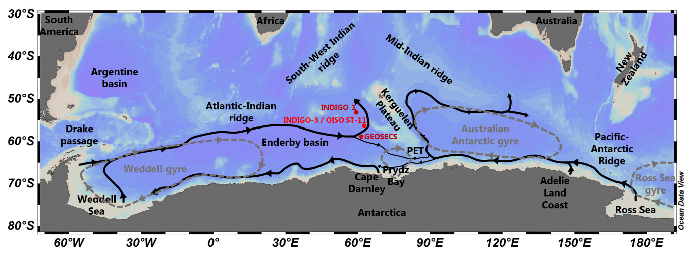
Figure 1 The rough AABW circulation transport paths from the literature (Orsi et al., 1999; Carter et al., 2008; Fukamachi et al., 2010; Williams et al., 2010; Vernet et al., 2019), with geographic indications (black text), main SO gyres (dark yellow text and dashed lines for the approximative locations) and stations considered in this study (red text and dots). PET: Princess Elizabeth Trough. Figure produced with Ocean Data View (Schlitzer, 2019).

The largest bottom water source of the global ocean is the Weddell Sea (Gordon et al., 2001). The exported WSDW is a mixture of the WSBW and Warm Deep Water (WDW). The WDW is a slightly modified Lower Circumpolar Deep Water (LCDW) by mixing with high-salinity surface water when the LCDW enters the Weddell basin (see Fig. 2 in van Heuven et al., 2011). The WSDW mixes with the LCDW during its transit. A part of the WSDW deflecting southward with the ACC in the Enderby Basin reaches the northwestern part of the Princess Elizabeth Trough (PET) region (area separating the Kerguelen Plateau from the Antarctic continent), where it mixes with other types of AABW (Heywood et al., 1999; Orsi et al., 1999). The deepest point of the PET is 3750 m, deep enough to allow AABW to flow between the Australian Antarctic Basin and the Enderby Basin (Heywood et al., 1999).

At the east of the PET, the CAC transports a mixture of RSBW and ALBW and accelerates northward along the eastern side of the Kerguelen Plateau (Mantyla and Reid, 1995; Fukamachi et al., 2010) following the Australian–Antarctic gyre, also called the Kerguelen gyre (Vernet et al., 2019). Part of the ALBW–RSBW mixture reaches the western side of the Kerguelen Plateau by the southern part of the PET (Heywood et al., 1999; Orsi et al., 1999; Van Wijk and Rintoul, 2014) and mixes with the CDBW. The mixture of CDBW and ALBW–RSBW flows westward with the CAC and dilutes with the LCDW (Meijers et al., 2010) until it reaches the Weddell gyre (Carter et al., 2008).

2.2 AABW definition

The distinction of water masses is usually performed according to neutral density (γⁿ) layers. In the SO, LCDW and AABW properties are generally well defined in the range 28.15–28.27 kg m⁻³ and 28.27 kg m⁻³ to the bottom, respectively (Orsi et al., 1999; Murata et al., 2019). However, to interpret the long-term variability of the properties in the AABW core at our location, we prefer to adjust the AABW definition to a narrow (more homogeneous) layer that we call Lower Antarctic Bottom Water (LAABW), characterized by γⁿ>28.35 kg m⁻³ (roughly ranging from 4200 to 4800 m; see Fig. 3). This definition corresponds to the AABW characteristics observed at higher latitudes in the Indian SO sector (Roden et al., 2016). The layer above the LAABW is hereafter called Upper Antarctic Bottom Water (UAABW).

3 Material and methods

3.1 AABW sampling during the last 40 years

Most of the data used in this study were obtained in the framework of the long-term observational project OISO (Ocean Indien Service d'Observations) conducted since 1998 onboard the R. S. V. Marion Dufresne (IPEV/TAAF). During these cruises, several stations are visited, but only one station is sampled down to the bottom (4800 m) south of the Polar Front, at 63.0^∘ E and 56.5^∘ S (hereafter denoted OISO-ST11). This station is located in the Enderby Basin on the western side of the Kerguelen Plateau (Fig. 1) and coincides with station 75 of the INDIGO-3 cruise (1987). In our analysis, we included all the data available for the OISO-ST11 location (which has not been sampled during each cruise for logistic reasons). We also included data from station 14 (deepest sample taken at 5109 m) of the INDIGO-1 cruise (1985) and station 430 (deepest sample taken at 4710 m) of the GEOSECS cruise (1978) located near the OISO-ST11 sampling site (405 and 465 km away from it, respectively; Fig. 1). All the reoccupations used in this analysis are listed in Table 1. Since seasonal variations are only observed in the surface mixed layer (Metzl et al., 2006), we used the observations available for all seasons (Table 1).

Table 1 List of the cruises used in this study.

3.2 Validation of the data

For 1998–2004, the OISO data were quality-controlled in CARINA (Lo Monaco et al., 2010) and for 2005 and 2009–2011 in GLODAPv2 (Key et al., 2015; Olsen et al., 2016, 2019). The three additional datasets from GEOSECS, INDIGO-1 and INDIGO-3 were first qualified in GLODAPv1 (Key et al., 2004) and used for the first C_ant estimates in the Indian Ocean (Sabine et al., 1999). The adjustments recommended for these historical datasets have been revisited in CARINA and GLODAPv2. In this paper we used the revised adjustments applied to the GLODAPv2 data product, with one exception for the total alkalinity (A_T) data from INDIGO-3 for which we applied an intermediate adjustment between the recommendation from GLODAPv1 (confirmed in CARINA) for no adjustment (due to a lack of available observations in this region for robust comparison) and the adjustment by −8 µmol kg⁻¹ applied to the GLODAPv2 data product (justification in the Supplement).

For the recent OISO cruises conducted in 2012–2018 not yet included in the most recent GLODAPv2 product, we have proceeded to a data quality control in deep water in which C_ant concentrations are low and subject to very small changes from year to year (see the Supplement).

3.3 Biogeochemical measurements

Measurement methods during OISO cruises were previously described (Jabaud-Jan et al., 2004; Metzl et al., 2006). In short, measurements were obtained using conductivity–temperature–depth (CTD) casts fixed on a 24 bottles rosette equipped with 12 L General Oceanics Niskin bottles. Potential temperature (Θ) and salinity (S) measurements have an accuracy of 0.002 ^∘C and 0.005, respectively. A_T and C_T were sampled in 500 mL glass bottles and poisoned with 100 µL of mercuric chloride saturated solution to halt biological activity. Discrete C_T and A_T samples were analyzed onboard by potentiometric titration derived from the method developed by Edmond (1970) using a closed cell. The repeatability for C_T and A_T varies from 1 to 3.5 µmol kg⁻¹ (depending on the cruise) and is determined by sample duplicates (at the surface, at 1000 m and in bottom water). The accuracy of C_T and A_T measurements (always better than ± 3 µmol kg⁻¹ for all cruises since 1998) was ensured by daily analyses of Certified Reference Materials (CRMs) provided by the A.G. Dickson laboratory (Scripps Institute of Oceanography). The dissolved oxygen (O₂) concentration was determined by an oxygen sensor fixed on the rosette. These values were adjusted using measurements obtained by Winkler titrations using a potentiometric titration system (at least 12 measurements for each profile). The thiosulfate solution used for the Winkler titration was calibrated using iodate standard solution (provided by Ocean Scientific International Limited) to ensure the standard O₂ accuracy of 2 µmol kg⁻¹. Nitrate (NO₃) and silicate (Si) concentrations were measured onboard or onshore with an automatic colorimetric Technicon analyzer following the methods described by Tréguer and Le Corre (1975) until 2008 and the revised protocol described by Coverly et al. (2009) since 2009. Based on replicate measurements for deep samples we estimate an error of about 0.3 % for both nutrients. NO₃ data are not available for all the cruises used in this analysis. The mean NO₃ concentration in the LAABW at OISO-ST11 is 32.8 ± 1.2 µmol kg⁻¹, while the average value derived from the GLODAP-v2 database in bottom water south of 50^∘ S in the southern Indian Ocean is 32.4 ± 0.6 µmol kg⁻¹. The lack of NO₃ data for few cruises has been palliated by using a climatological value of 32.4 µmol kg⁻¹ with a limited impact on C_ant determined by the C^∘ method (<2 µmol kg⁻¹ for estimates based on the differences observed between NO₃ measurements and the climatological value).

3.4 C_ant calculation using the TrOCA method

The TrOCA method was first presented by Touratier and Goyet (2004a, b) and revised by Touratier et al. (2007). Following the concept of the quasi-conservative tracer NO (Broecker, 1974), TrOCA is a tracer defined as a combination of O₂, C_T and A_T following

$$\begin{array}{}\text{(1)}& \mathrm{TrOCA}={\mathrm{O}}_{\mathrm{2}}+a\left(C_{\mathrm{T}}-{\displaystyle \frac{\mathrm{1}}{\mathrm{2}}}{A}_{\mathrm{T}}\right),\end{array}$$

where a is defined in Touratier et al. (2007) as a combination of the Redfield equation coefficients for CO₂, O₂, HPO${}_{\mathrm{4}}^{\mathrm{2}-}$ and H⁺. For more details about the definition and the calibration of this parameter, please refer to Touratier et al. (2007). The temporal change in TrOCA is independent of biological processes and can be attributed to anthropogenic carbon (Touratier and Goyet, 2004a). Therefore, C_ant can be directly calculated from the difference between TrOCA and its preindustrial value TrOCA^∘:

$$\begin{array}{}\text{(2)}& C_{\mathrm{ant}}={\displaystyle \frac{\mathrm{TrOCA}-{\mathrm{TrOCA}}^{\mathrm{0}}}{a}},\end{array}$$

where TrOCA^∘ is evaluated as a function of Θ and A_T (Eq. 3) as

$$\begin{array}{}\text{(3)}& {\mathrm{TrOCA}}^{\mathrm{0}}=e^{\left[b-\left(c\right)\mathrm{\Theta }-\frac{d}{A_{\mathrm{T}}^{\mathrm{2}}}\right]}.\end{array}$$

In these expressions, the coefficients a, b, c and d were adjusted by Touratier et al. (2007) from deep water free of anthropogenic CO₂ using the tracers Δ¹⁴C and CFC-11 from the GLODAPv1 database (Key et al., 2004). The final expression used to calculate C_ant is

$$\begin{array}{}\text{(4)}& C_{\mathrm{ant}}={\displaystyle \frac{{\mathrm{O}}_{\mathrm{2}}+\mathrm{1.279}\left(C_{\mathrm{T}}-\frac{\mathrm{1}}{\mathrm{2}}{A}_{\mathrm{T}}\right)-e^{\left[\mathrm{7.511}-\left({\mathrm{1.087.10}}^{-\mathrm{2}}\right)\mathrm{\Theta }-\frac{{\mathrm{7.81.10}}^{\mathrm{5}}}{A_{\mathrm{T}}^{\mathrm{2}}}\right]}}{\mathrm{1.279}}}.\end{array}$$

The consideration of the errors on the different parameters involved in the TrOCA method results in an uncertainty of ± 6.25 µmol kg⁻¹ (mostly due to the parameter a, leading to ± 3.31 µmol kg⁻¹). As this error is relatively large compared to the expected C_ant concentrations in deep and bottom SO water (Pardo et al., 2014) we will compare the TrOCA results using another indirect method to interpret C_ant changes over 40 years.

3.5 C_ant calculation using the preformed inorganic carbon (C⁰) method

To support the C_ant trend determined with the TrOCA method, C_ant was also estimated using a back-calculation approach denoted C⁰ (Brewer, 1978; Chen and Millero, 1979), previously adapted for C_ant estimates along the WOCE-I6 section between South Africa and Antarctica (Lo Monaco et al., 2005a). This method consists of the correction of the measured C_T for the biological contribution (C_bio) and preindustrial preformed C_T ($C_{\mathrm{PI}}^{\mathrm{0}}$):

$$\begin{array}{}\text{(5)}& C_{\mathrm{ant}}=C_{\mathrm{T}}-C_{\mathrm{bio}}-C_{\mathrm{PI}}^{\mathrm{0}}.\end{array}$$

C_bio (Eq. 6) depends on carbonate dissolution and organic matter remineralization, taking account of the corrected C∕O₂ ratio from Körtzinger et al. (2001):

$$\begin{array}{}\text{(6)}& C_{\mathrm{bio}}=\mathrm{0.5}\mathrm{\Delta }{A}_{\mathrm{T}}-\left(\mathrm{C}/{\mathrm{O}}_{\mathrm{2}}+\mathrm{0.5}\mathrm{N}/{\mathrm{O}}_{\mathrm{2}}\right)\mathrm{\Delta }{\mathrm{O}}_{\mathrm{2}},\end{array}$$

where $\mathrm{C}/{\mathrm{O}}_{\mathrm{2}}=\mathrm{106}/\mathrm{138}$ and $\mathrm{N}/{\mathrm{O}}_{\mathrm{2}}=\mathrm{16}/\mathrm{138}$. ΔA_T and ΔO₂ are the difference between the measured values (A_T and O₂) and the preformed values ($A_{\mathrm{T}}^{\mathrm{0}}$ and O${}_{\mathrm{2}}^{\mathrm{0}}$). $A_{\mathrm{T}}^{\mathrm{0}}$ (Eq. 7) has been computed by Lo Monaco et al. (2005a) as a function of Θ, S and the conservative tracer PO:

$$\begin{array}{}\text{(7)}& A_{\mathrm{T}}^{\mathrm{0}}=\mathrm{0.0685}\mathrm{PO}+\mathrm{59.79}S-\mathrm{1.45}\mathrm{\Theta }+\mathrm{217.1}.\end{array}$$

PO (Eq. 8) has been defined by Broecker (1974) and depends on the equilibrium of O₂ with phosphate (PO₄). When PO₄ data are not available, nitrate (NO₃) can be used instead as follows (the N∕P ratio of 16 is from Anderson and Sarmiento, 1994):

$$\begin{array}{}\text{(8)}& \mathrm{PO}={\mathrm{O}}_{\mathrm{2}}+\mathrm{170}{\mathrm{PO}}_{\mathrm{4}}={\mathrm{O}}_{\mathrm{2}}+(\mathrm{170}/\mathrm{16}){\mathrm{NO}}_{\mathrm{3}}.\end{array}$$

To determine O${}_{\mathrm{2}}^{\mathrm{0}}$, it is assumed that the surface water is in full equilibrium with the atmosphere (O${}_{\mathrm{2}}^{\mathrm{0}}=$ O_2,sat; Benson and Krause, 1980) and that after subduction O₂ in a given water mass is only impacted by the biological activity (Weiss, 1970). A correction of O${}_{\mathrm{2}}^{\mathrm{0}}$ has been proposed by Lo Monaco et al. (2005a) to take account of the undersaturation of O₂ due to sea ice cover at high latitudes. O${}_{\mathrm{2}}^{\mathrm{0}}$ is therefore corrected by assuming a mean mixing ratio of the ice-covered surface water k=50 % (Lo Monaco et al., 2005a) and a mean value for O₂ undersaturation in ice-covered surface water α=12 % (Anderson et al., 1991) according to Eq. (9):

$$\begin{array}{}\text{(9)}& \mathrm{\Delta }{\mathrm{O}}_{\mathrm{2}}=(\mathrm{1}-\mathit{\alpha }k){\mathrm{O}}_{\mathrm{2},\mathrm{sat}}-{\mathrm{O}}_{\mathrm{2}}=\mathrm{AOU}.\end{array}$$

$C_{PI}^{\mathrm{0}}$ in Eq. (5) is a function of the current preformed C_T ($C_{\mathrm{obs}}^{\mathrm{0}}$) and a reference water term (Eq. 10):

$$\begin{array}{}\text{(10)}& C_{\mathrm{PI}}^{\mathrm{0}}=C_{\mathrm{obs}}^{\mathrm{0}}+{\left[C_{\mathrm{T}}-C_{\mathrm{bio}}-C_{\mathrm{obs}}^{\mathrm{0}}\right]}_{\mathrm{REF}}.\end{array}$$

$C_{\mathrm{obs}}^{\mathrm{0}}$ has been computed similarly as $A_{\mathrm{T}}^{\mathrm{0}}$ (Eq. 11):

$$\begin{array}{}\text{(11)}& C_{\mathrm{obs}}^{\mathrm{0}}=-\mathrm{0.0439}\mathrm{PO}+\mathrm{42.79}S-\mathrm{12.02}\mathrm{\Theta }+\mathrm{739.8},\end{array}$$

where the reference water term is a constant for a given time of observation corresponding to the time when $C_{\mathrm{obs}}^{\mathrm{0}}$ is parameterized. In this paper, we used the parameterization given by Lo Monaco et al. (2005a) and their estimated value for the reference term of 51 µmol kg⁻¹. This number has been computed using an optimum multiparametric (OMP) model to estimate the mixing ratio of the North Atlantic deep water in the SO (used as reference water, i.e., old water mass, where C_ant=0). For more details about the C⁰ method, which has a final error of ± 6 µmol kg⁻¹, please see Lo Monaco et al. (2005a).

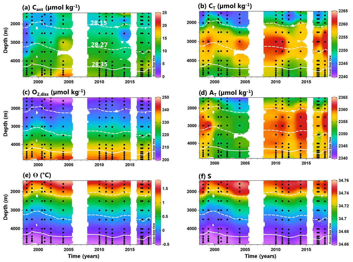
Figure 2 Hovmöller diagram of (a) C_ant via TrOCA, (b) C_T, (c) O₂, (d) A_T, (e) Θ and (f) S based on the OISO data presented in Table 1. Data points are represented by black dots. The white isolines represent the water mass separation by γⁿ (from the bottom: LAABW, UAABW and LCDW). Figure produced with Ocean Data View (Schlitzer, 2019).

4 Results

The vertical distribution of hydrological and biogeochemical properties observed in deep and bottom water and their evolution over the last 40 years are displayed in Fig. 2. The LCDW layer (γⁿ=28.15–28.27 kg m⁻³) is characterized by minimum O₂ concentrations (Fig. 2c), higher C_T (Fig. 2b) and lower C_ant concentrations than the AABW (Fig. 2a). C_ant concentrations were not significant in the LCDW until the end of the 1990s (<6 µmol kg⁻¹); then our data show an increase in C_ant between the two 1998 reoccupations, followed by relatively constant C_ant concentrations (10 ± 3 µmol kg⁻¹). In the LAABW (γⁿ>28.35 kg m⁻³), well identified by low Θ, low S and high O₂, C_ant concentrations are higher than in the overlying UAABW and LCDW (Fig. 2a). The evolutions of the mean properties in the LAABW over 40 years are shown in Fig. 3. In this layer, C_ant concentrations increased from 5 ± 4 µmol kg⁻¹ in 1978 and 7 ± 4 µmol kg⁻¹ in the mid-1980s to 13 ± 2 µmol kg⁻¹ at the end of the 1990s and up to 19 ± 2 µmol kg⁻¹ in 2004 (Fig. 3a). Figure 3a also shows a very good agreement between the TrOCA method and the C⁰ method for both the magnitude and variability of C_ant in the LAABW. Our results show a mean C_ant trend in the LAABW of +1.4 µmol kg⁻¹ per decade over the full period and a maximum trend of the order of +5.2 µmol kg⁻¹ per decade over 1987–2004 (Table 2). Due to the mixing of AABW with old LCDW (C_ant free), these trends are lower than the theoretical trend expected from the increase in atmospheric CO₂. Indeed, assuming that the surface ocean fCO₂ follows the atmospheric growth rate (+1.8 µatm yr⁻¹ over 1978–2018) in the seasonal ice zone (Roden et al., 2016), the theoretical C_ant trend at AABW formation sites would be of the order of +8 µmol kg⁻¹ per decade in the Antarctic surface water. This is close to the theoretical C_T trend estimated for freezing shelf water in the Weddell Sea (van Heuven et al., 2014).

Figure 3 Interannual variability (dashed lines) and significant trends (at 95 %, see Table 2; dotted lines) for the 40 years of observation of the OISO-ST11 LAABW properties, including (a) C_ant by the TrOCA (black circles and triangles) and the C⁰ (open circles) method, (b) C_T (black circles) and C_nat (open circles), (c) O₂, (d) A_T, (e) Θ, and (f) S. For (a) C_ant, (b) C_nat and (d) A_T, the triangles pointing up and down correspond to INDIGO-3 values with and without −8 µmol kg⁻¹ of correction on the A_T, respectively (see the Supplement for more details).

Table 2 Trends (per decade) of observed and calculated properties in the LAABW estimated over different periods (in bold: significant trends at the 95 % confidence level).

Over the full period, C_T increased by 2.0 ± 0.5 µmol kg⁻¹ per decade, mostly due to the accumulation of C_ant (Table 2). Our data also show a significant decrease in O₂ concentrations by 0.8 ± 0.4 µmol kg⁻¹ per decade over the 40-year period (Fig. 3c, Table 2) that could be caused by reduced ventilation, as suggested by Schmidtko et al. (2017), who observed significant O₂ loss in the global ocean. In the deep Indian SO sector, these authors found a trend approaching −1 µmol kg⁻¹ per decade over 50 years (1960–2010), which is consistent with our data. We did not detect any significant trend in A_T, Θ and S over the full period, but over shorter periods our data show a significant decrease in A_T. The low A_T values observed over 2000–2004 (Fig. 3d) could suggest reduced calcification in the upper ocean, leading to less sinking of calcium carbonate tests and a decrease in A_T in deep and bottom water over this period (Fig. 2d). For this period the increase in C_T was lower than the accumulation of C_ant, but such a feature is disputable in view of the uncertainty on the C_ant calculation. This event is followed by an increase in the “natural” component of C_T (C_nat, calculated as the difference between C_T and C_ant) since 2004 associated with a decrease in O₂ and no increase in C_ant (Table 2). These trends were not associated with a significant trend in Θ or S (Fig. 3e, f, Table 2). The increase in C_nat is thus unlikely to originate from increased mixing with LCDW during bottom water transport, confirming that our LAABW definition excludes mixing with the LCDW. Enhanced organic matter remineralization is also unlikely since NO₃ did not show any significant trend (Table 2).

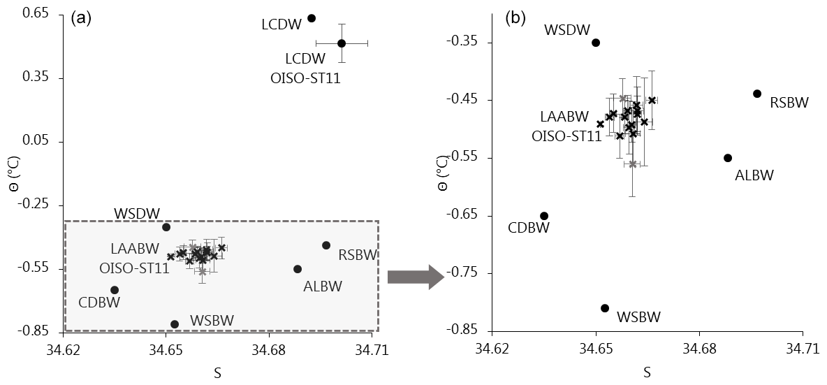
Figure 4 (a) Full Θ–S diagram of studied water masses and (b) a zoom-in to bottom water. Values are from the literature for the WSBW (Fukamachi et al., 2010; van Heuven, 2013; Pardo et al., 2014; Robertson et al., 2002), the WSDW (Carmack and Foster, 1975; Fahrbach et al., 1994; van Heuven, 2013; Robertson et al., 2002), the RSBW (Fukamachi et al., 2010; Gordon et al., 2015; Johnson, 2008; Pardo et al., 2014), the ALBW (Fukamachi et al., 2010; Johnson, 2008; Pardo et al., 2014), the CDBW (Ohshima et al., 2013) and the LCDW (Lo Monaco et al., 2005a; Pardo et al., 2014; Smith and Treguer, 1994), as well as from the OISO-ST11 dataset for the OISO-ST11 LAABW and OISO-ST11 LCDW. Error bars are calculated from the individual annual averaged values for the OISO-ST11 LAABW and from all data for the OISO-ST11 LCDW. For the OISO-ST11 LAABW, the grey cross are the GEOSECS (lowest Θ) and INDIGO-1 (highest Θ) values.

Importantly, our data show substantial interannual variations in LAABW properties, which could significantly impact the trends estimated from limited reoccupations (e.g., Williams et al., 2015; Pardo et al., 2017; Murata et al., 2019). For example, we found relatively higher C_ant concentrations in 1985 (10 µmol kg⁻¹) compared to 1978 (5 µmol kg⁻¹) and 1987 (7 µmol kg⁻¹). This is linked to a signal of low S in 1985 (Fig. 3f) that could be due to a larger contribution of fresher water such as the WSDW or CDBW. This could also be related to the different sampling locations. Over the last decade (2009–2018), our data show large and rapid changes in S that are partly reflected in C_T and O₂ and that could explain the relatively low C_ant concentrations observed over this period. Indeed, the S maximum observed in 2012 (correlated to higher Θ) is associated with a marked C_T minimum (surprisingly almost as low as in 1987), as well as low A_T (hence low C_nat) and low NO₃ concentrations. Since these anomalies were associated with a decrease in C_ant concentrations, one may argue for an increased contribution of bottom water ventilated far away from our study site. A few years later our data show an S minimum (correlated with lower Θ) associated with a rapid increase in C_T and a rapid decrease in O₂ between 2013 and 2016, suggesting the contribution of a closer AABW type such as the CDBW. The freshening of −0.006 per decade in S between 2004 and 2018 that we observed on the western side of the Kerguelen Plateau was also observed on the eastern side of the plateau by Menezes et al. (2017) over a similar period. In this region, Menezes et al. (2017) evaluated a change in S by about −0.008 per decade from 2007 to 2016 (against −0.002 per decade between 1994 and 2007), suggesting an acceleration of AABW freshening in recent years. However, they also reported a warming by +0.06 ^∘C per decade, while we observed cooler temperatures in 2016–2018. This suggests that we sampled a different mixture of AABW.

5 Discussion

5.1 LAABW composition at OISO-ST11

At each formation site, AABW experiences significant temporal property changes, mostly recognized at a decadal scale (e.g., freshening in the southern Indian Ocean; Menezes et al., 2017), with a potential impact on carbon uptake and C_ant concentrations during AABW formation (Shadwick et al., 2013). The Θ–S diagram constructed from yearly averaged data in bottom water (Fig. 4) shows that the LAABW at OISO-ST11 is a complex mixture of WSDW, CDBW, RSBW and ALBW. The coldest type of LAABW was observed at the GEOSECS station at 60^∘ S (−0.56 ^∘C), while the warmer type of LAABW was observed at the INDIGO-1 station at 53^∘ S (−0.44 ^∘C). These extreme Θ values could be a natural feature or may be related to specific sampling. For the other cruises, Θ in LAABW ranges from −0.51 to −0.45 ^∘C with no clear indication of the specific AABW origin. The S range observed in the bottom water at OISO-ST11 (34.65–34.67) illustrates either changes in mixing with various AABW sources or temporal variations at the formation site. Given knowledge of deep and bottom water circulation and characteristics (Figs. 1 and 4) and the significant C_ant concentrations that we calculated in the LAABW (Fig. 3a), the main contribution at our location is likely the younger and colder CDBW for which relatively high C_ant concentrations have been recently documented (Roden et al., 2016). From its formation region, the CDBW can either flow westward with the CAC or flow northward in the Enderby Basin (Ohshima et al., 2013; Fig. 1). In the CAC branch, the CDBW mixes with the LCDW along the Antarctic shelf and the continental slope between 80 and 30^∘ E (Meijers et al., 2010; Roden et al., 2016). On the western side of the Kerguelen Plateau, CDBW also mixes with RSBW and ALBW (Orsi et al., 1999; Van Wijk and Rintoul, 2014). In this context, the C_ant concentrations observed in the bottom layer at OISO-ST11 are probably not linked to one single AABW source but are likely a complex interplay of AABW from different sources with different biogeochemical properties.

5.2 C_ant concentrations

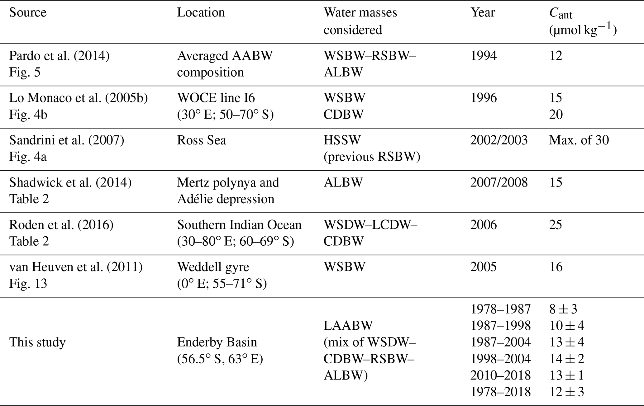
In order to compare our C_ant estimates with other studies, we separated the 40-year time series into three periods: the first period (1978–1987) corresponds to historical data when C_ant is expected to be low; the second period (1998–2004) starts when the first OISO cruise was conducted (using CRMs for A_T and C_T measurements) and ends when C_ant concentrations in the LAABW are maximum (Fig. 3a); and the third period consists of the observations performed in late 2009 to 2018 when the observed variations are relatively large for S and small for C_ant. The mean C_ant concentrations for each period are 7, 14 and 13 µmol kg⁻¹, respectively, which is consistent with the results from other studies (Table 3). The C_ant values for 1978–1987 can hardly be compared to other studies because very few observations were conducted in the 1980s in the Indian sector of the SO (Sabine et al., 1999) and because of potential biases for historical data despite their careful quality control in GLODAP and CARINA (Key et al., 2004; Lo Monaco et al., 2010; Olsen et al., 2016). In addition, the different methods used to estimate C_ant can lead to different results, especially in deep and bottom water of the SO (Vázquez-Rodríguez et al., 2009). Overall, Table 3 confirms that C_ant concentrations were low in the 1970s and 1980s and reached values of the order of 10 µmol kg⁻¹ in the 1990s, a signal not clearly captured in global data-based estimates (Gruber, 1998; Sabine et al., 2004; Waugh et al., 2006; Khatiwala et al., 2013).

Table 3 Compilation of C_ant sequestration investigations in the AABW (γⁿ≥28.25 kg m⁻³) using the TrOCA method. The C_ant estimation of Pardo et al. (2014) is calculated using theoretical AABW mean composition (with 3 % of ALBW) and the carbon data from the GLODAPv1 and CARINA databases. Sandrini et al. (2007) values have been measured at the bottom of the Ross Sea and correspond to recently sinking high-salinity shelf water (HSSW). The mean values published by Roden et al. (2016) for the AABW present WSDW characteristics but can be a mix of CDBW and LCDW.

The observations presented in this analysis, although regional, offer a complement to recent estimates of C_ant changes evaluated between 1994 and 2007 in the top 3000 m for the global ocean (Gruber et al., 2019a). In the Enderby Basin at the horizon at 2000–3000 m, the accumulation of C_ant from 1994 to 2007 is not uniform and ranges between 0 and 8 µmol kg⁻¹ (Gruber et al., 2019a). At our station, in the LCDW (2000–3000 m) the C_ant concentrations were not significant in 1978–1987 (−2 to 5 µmol kg⁻¹) but increase to an average of 9 ± 3 µmol kg⁻¹ in 1998–2018 (Fig. 2a), probably due to mixing with AABW that contains more C_ant. Interestingly, this value is close but in the high range of the C_ant accumulation estimated from 1994 to 2007 in deep water of the southern Indian Ocean (Gruber et al., 2019a).

Not surprisingly, high C_ant concentrations are detected in the AABW formation regions (Table 3). The highest C_ant concentrations in bottom water (up to 30 µmol kg⁻¹) were observed in the ventilated shelf water in the Ross Sea (Sandrini et al., 2007). In the Adélie and Mertz polynya regions, Shadwick et al. (2014) observed high C_ant concentrations in the subsurface shelf water (40–44 µmol kg⁻¹) but lower values in the ALBW (15 µmol kg⁻¹) due to mixing with older LCDW. In WSBW, all C_ant concentrations estimated from observations between 1996 and 2005 and with the TrOCA method (Table 3) lead to about the same values ranging between 13 and 16 µmol kg⁻¹ (Lo Monaco et al., 2005b; van Heuven et al., 2011). In bottom water formed near Cape Darnley (CDBW), Roden et al. (2016) estimated high C_ant concentrations in bottom water (25 µmol kg⁻¹) resulting from the shelf water that contains very high amounts of C_ant (50 µmol kg⁻¹). The comparison with other studies confirms that far from the AABW formation sites, contemporary C_ant concentrations do not exceed 16 µmol kg⁻¹ on average.

5.3 C_ant trends and variability

Comparison of long-term C_ant trends in deep and bottom water of the SO is limited to very few regions where repeated observations are available. To our knowledge, only three other studies have evaluated the long-term C_ant trends in the SO based on more than five reoccupations: in the southwestern Atlantic (Ríos et al., 2012) and in the Weddell gyre along the prime meridian section (van Heuven et al., 2011, 2014). Temporal changes in C_T and C_ant have also been investigated in other SO regions but limited to two to four reoccupations (Williams et al., 2015; Pardo et al., 2017; Murata et al., 2019). Given the C_ant variability depicted at our location (Fig. 3a), different trends can be deduced from limited reoccupations. As an example, Murata et al. (2019) evaluated the change in C_ant from data collected 17 years apart (1994–1996 and 2012–2013) along a transect around 62^∘ S and found a small increase at our location (<5 µmol kg⁻¹ around 60^∘ E). This result appears very sensitive to the time of the observation given that we found a minimum in C_ant concentrations between 2011 and 2014 (Fig. 3a) associated with a marked C_T minimum (Fig. 3b). In addition, our results show that the detection of C_ant trends appears very sensitive to the time period considered (Table 2). As an extreme case, the C_ant trend calculated for the period 1987–2004 is +5.2 µmol kg⁻¹ per decade (relatively close to the theoretical C_ant trend of +8 µmol kg⁻¹ per decade), but it reverses to −3.5 µmol kg⁻¹ per decade for the period 2004–2018.

The long-term C_T trend that we estimated in the LAABW in the eastern Enderby Basin (2.0 ± 0.5 µmol kg⁻¹ per decade) is slightly faster than the C_T trends estimated in the WSBW in the Weddell gyre: +1.2 ± 0.5 µmol kg⁻¹ per decade over the period 1973–2011 and +1.6 ± 1.4 µmol kg⁻¹ per decade when restricted to 1996–2011 (van Heuven et al., 2014). Along the SR03 line (south of Tasmania) reoccupied in 1995, 2001, 2008 and 2011, Pardo et al. (2017) calculated a C_T trend of +2.4 ± 0.2 µmol kg⁻¹ per decade in the AABW, composed of ALBW and RSBW in this sector. This is higher than the C_T trends found at our location and in the Weddell gyre, but surprisingly, this was not associated with a significant increase in C_ant. The C_T trend in AABW along the SR03 section was likely due to the intrusion of old and C_T-rich water also revealed by an increase in Si concentrations during 1995–2011 (Pardo et al., 2017). This is a clear example of decoupling between C_T and C_ant trends in deep and bottom water as observed at our location in the last decade (Table 2). For C_ant, our 40-year trend estimate (1.4 ± 0.5 µmol kg⁻¹ per decade) appears close to the trend reported by Ríos et al. (2012) in the southwestern Atlantic AABW from six reoccupations between 1972 and 2003 (+1.5 µmol kg⁻¹ per decade). However, if we limit our result to the period 1978–2002 or 1978–2004 (about the same period as in Ríos et al., 2012), our trend is much larger (+3–4 µmol kg⁻¹ per decade).

At our location, the C_ant trend over 40 years (+1.4 ± 0.5 µmol kg⁻¹ per decade) explains most of the observed C_T increase (+2.0 ± 0.5 µmol kg⁻¹ per decade). The residual of +0.4 µmol kg⁻¹ per decade reflects changes in natural processes affecting the carbon content (different AABW sources, ventilation, mixing with deep water, remineralization or carbonates dissolution). Although this is a weak signal, the natural C_T change (C_nat) mirrors the observed decrease in O₂ by $-\mathrm{0.8}\pm$ 0.4 µmol kg⁻¹ per decade. This O₂ decrease detected in the Enderby Basin appears to be a real feature that was documented at a large scale for 1960–2010 in deep SO basins (Schmidtko et al., 2017), suggesting that the changes observed at 63^∘ E, 56.5^∘ S are related to large-scale processes, possibly due to a decrease in AABW formation (Purkey and Johnson, 2012).

5.4 Recent C_ant stability

Although most studies suggest a gradual accumulation of C_ant in the AABW, our time series highlights significant multi-annual changes, in particular over the last decade when C_ant concentrations were as low as around the year 2000 (Fig. 3a) and decoupled from the increase in C_T (Fig. 3b). This result is difficult to interpret because at our location, away from AABW sources (Fig. 1), the temporal variability observed in the LAABW layer can result from many remote processes occurring at the AABW formation sites (such as wind forcing, ventilation, sea ice melting, thermodynamic, biological activity and air–sea exchanges). Additionally, internal processes during the transport of AABW (such as organic matter remineralization, carbonate dissolution and mixing with surrounding water) must also be taken into account. The apparent steady C_ant feature suggests that AABW found at our location has stored less C_ant in recent years. This might be linked to reduced CO₂ uptake in the AABW formation regions, as recognized at a large scale in the SO from the late 1980s to 2001 (Le Quéré et al., 2007; Metzl, 2009; Lenton et al., 2012; Landschützer et al., 2015). This large-scale response in the SO during a positive trend in the Southern Annular Mode (SAM) is mainly associated with stronger winds driven by accelerating greenhouse gas emissions and stratospheric ozone depletion, leading to warming and freshening in the SO (Swart et al., 2018), a change in the ventilation of C_T-rich deep water, and reduced CO₂ uptake (Lenton et al., 2009). The reconstructed pCO₂ fields by Landschützer et al. (2015) suggest that the reduced CO₂ sink in the 1990s is identified at high latitudes in the SO (see Figs. 2a and S9 in Landschützer et al., 2015). However, as opposed to the circumpolar open ocean zone (e.g., Metzl, 2009; Takahashi et al., 2009, 2012; Munro et al., 2015; Fay et al., 2018), the long-term trend of surface fCO₂ and carbon uptake deduced from direct observations is not clearly identified in the seasonal ice zone (SIZ), the shelves around Antarctica, and thus in the AABW formation regions of interest to interpret our results (Laruelle et al., 2018). There, surface fCO₂ data are sparse, especially before 1990, and cruises were mainly conducted in austral summer when the spatiotemporal fCO₂ variability is very large and driven by multiple processes at regional or small scales, such as primary production, sea ice formation and retreat, and water circulation and mixing. This leads to various estimates of the air–sea CO₂ fluxes around Antarctica depending on the region and period and large uncertainty when attempting to detect long-term trends (Gregor et al., 2018).

In particular, in polynyas and AABW formation regions where fCO₂ is low and where katabatic winds prevail, a very strong instantaneous CO₂ sink can occur at the local scale (up to −250 mmol C m⁻² d⁻¹ in Terra Nova Bay in the Ross Sea according to DeJong and Dunbar, 2017). In the Prydz Bay region where CDBW is formed, recent studies show that surface fCO₂ in austral summer varies over a very large range (150–450 µatm), with the lowest fCO₂ observed in the shelf region generating a very strong local CO₂ sink (−221 mmol C m⁻² d⁻¹; Roden et al., 2016). The carbon uptake was particularly enhanced near Cape Darnley and coincided with the highest C_ant concentrations that Roden et al. (2016) estimated in the dense shelf water that subducts to form AABW. In the Prydz Bay coastal region, surface fCO₂ values in 1993–1995 were as low as 100 µatm (Gibson and Trull, 1999), leading to a strong local CO₂ uptake of −30 mmol C m⁻² d⁻¹ in summer. In addition, Roden et al. (2013) found a large C_T increase over 16 years (+34 µmol kg⁻¹) in the Prydz Bay, which is much higher than the anthropogenic signal alone (+12 µmol kg⁻¹) and likely explained by changes in primary production that would have been stronger in 1994. To our knowledge, this is the only direct observation of decadal C_T change in surface water in a region of AABW formation (here the Prydz Bay), and it highlights the difficulty not only of evaluating the C_T and C_ant long-term trends in these regions but also separating natural and anthropogenic signals when this water reaches the deep ocean. We attempted to detect long-term changes in CO₂ uptake in this region using the qualified fCO₂ data available in the SOCAT database (Bakker et al., 2016), but our estimates (not shown) were highly uncertain due to very large spatial and temporal variability. To conclude, all previous studies conducted near or in AABW formation sites clearly reveal that these regions are potentially strong carbon sinks, but how the sink changed over the last decades is not yet evaluated, and thus we are not able to certify that the recent C_ant stability that we observed in the LAABW at our location is directly linked to the weakening of the carbon sink that was recognized at the large scale in the SO from the 1980s to mid-2000s (Le Quéré et al., 2007; Landschützer et al., 2015).

Changes in the accumulation of C_ant in AABW could also be directly related to changes in physical processes occurring in AABW formation regions. Decadal decreasing of sea ice production and melting of sea ice have been documented in several regions, including Cape Darnley polynyas (Tamura et al., 2016; Williams et al., 2016). The consequent changes in Antarctic surface water properties are transmitted into the deep ocean, notably the well-recognized freshening of the AABW (Rintoul, 2007; Anilkumar et al., 2015). The warming of bottom water was also documented in the Enderby Basin (Couldrey et al., 2013) as well as at a larger scale in all deep SO basins (Purkey and Johnson, 2010; Desbruyères et al., 2016). Associated with a decrease in AABW formation in the 1990s (Purkey and Johnson, 2012), these physical changes could explain the recent stability of C_ant concentrations in AABW observed at our location. As AABW from different sources spreads and mixes with C_T-rich deep water before reaching our location (Fig. 1), less AABW formation and export would result in an increase in C_T (increase in C_nat) not associated with an increase in C_ant and a decrease in O₂ (as observed in recent years in Fig. 3a, b, c). Finally, it is also possible that the LAABW observed in recent years at our location is the result of a larger contribution of older RSBW, ALBW or even WSBW that has lower C_ant and O₂ concentrations compared to CDBW formed at Cape Darnley and Prydz Bay.

6 Conclusions

The distribution and evolution of C_ant in the bottom layer of the SO are related to complex interactions between climatic forcing, air–sea CO₂ exchange at formation sites, and biological and physical processes during AABW circulation. The dataset that we collected regularly in the Enderby Basin over the last 20 years (1998–2018) in the framework of the OISO project, together with historical observations obtained in 1978, 1985 and 1987 (GEOSECS and INDIGO cruises), allows for the investigation of C_ant changes in AABW over 40 years in this region. The focus on AABW variability is made by defining Lower Antarctic Bottom Water (LAABW) as described in Sect. 2.3. Our results suggest that the accumulation of C_ant explains most, but not all, of the observed increase in C_T. We also detected a decrease in O₂ that is consistent with the large-scale signal reported by Schmidtko et al. (2017), possibly due to a decrease in AABW formation (Purkey and Johnson, 2012). Our data further indicate rapid anomalies in some periods, suggesting that for decadal to long-term estimates care has to be taken when analyzing the change in C_ant from datasets collected 10 or 20 years apart (e.g., Williams et al., 2015; Murata et al., 2019). Our results also show different C_ant trends over short periods, with a maximum increase of 5.2 µmol kg⁻¹ per decade between 1987 and 2004 and apparent stability in the last 20 years (despite an increase in C_T). This suggests that AABW has stored less C_ant in the last decade, but our understanding of the processes that explain this signal is not clear. This might be the result of the reduced CO₂ uptake in the SO in the 1990s (Le Quéré et al., 2007; Landschützer et al., 2015), but this is not yet verified from direct C_T or fCO₂ observations in AABW formation regions due to the lack of winter data and very large variability during summer. This calls for more data collection and investigations in these regions. The apparent stability of C_ant in the LAABW since 1998 could also be directly linked to a decrease in AABW formation in the 1990s (Purkey and Johnson, 2012) or a change in the contributions of AABW from different sources, especially in the Prydz Bay region (Williams et al., 2016). In these scenarios, an increased contribution of C_T-rich and O₂-poor older LCDW along AABW transit would also explain the decoupling between C_ant and C_T (increase in C_nat) and decrease in O₂ concentrations observed in recent years, even if we tried to isolate this specific feature in our data selection. The decoupling between C_ant and C_T is not a unique feature, as it was also reported along the SR03 section between Tasmania and Antarctica, most probably due to advection of C_T-rich water (Pardo et al., 2017). This highlights the importance of the ocean circulation in influencing temporal C_T and C_ant inventory changes (De Vries et al., 2017) and the need to better separate anthropogenic and natural variability based on time series observations.

The evaluation and understanding of decadal C_ant changes in deep and bottom ocean water are still challenging, as the C_ant concentrations remain low compared to C_T measurement accuracy (at best ± 2 µmol kg⁻¹, Bockmon and Dickson, 2015) and uncertainties of data-based methods (± 6 µmol kg⁻¹). Long-term repeated and qualified observations (at least 30 years) are needed to accurately detect and separate the anthropogenic signal from the internal ocean variability; we are thus only starting to document these trends that should now help to identify shortcomings in models regarding carbon storage in the deep SO (e.g., Frölicher et al., 2015). As changes in the SO (including warming, freshening, oxygenation and deoxygenation, CO₂, and acidification) are expected to accelerate in the future in response to anthropogenic forcing and climate change (e.g., Heuzé et al., 2015; Hauck et al., 2015; Ito et al., 2015; Yamamoto et al., 2015), it is important to maintain time series observations to complement the GO-SHIP strategy and to more regularly occupy other sectors of the SO (Rintoul et al., 2012). In this context, we hope to maintain our observations in the southern Indian Ocean in the next decade, and with ongoing synthetic product activities such as GLODAPv2 (Olsen et al., 2016, 2019), SOCAT (Bakker et al., 2016) and more recently the SOCCOM project (Williams et al., 2018), to offer a solid database to validate ocean biogeochemical models and coupled climate–carbon models (Russell et al., 2018) and ultimately reduce uncertainties in future climate projections.