the Creative Commons Attribution 4.0 License.
the Creative Commons Attribution 4.0 License.
 | 11 Dec 2020
Assessment of responses of North Atlantic winter sea surface temperature to the North Atlantic Oscillation on an interannual scale in 13 CMIP5 models
Yujie Jing
Yangchun Li
Yongfu Xu
This study evaluates the response of winter-average sea surface temperature (SST) to the winter North Atlantic Oscillation (NAO) simulated by 13 Coupled Model Intercomparison Project Phase 5 (CMIP5) Earth system models in the North Atlantic (NA) (0–65∘ N) on an interannual scale. Most of the models can reproduce an observed tripolar pattern of the response of the SST anomalies to the NAO on an interannual scale. The model bias is mainly reflected in the locations of the negative-response centers in the subpolar NA (45–65∘ N), which is mainly caused by the bias of the response of the SST anomalies to the NAO-driven turbulent heat flux (THF) anomalies. Although the influence of the sensible heat flux (SHF) on the SST is similar to that of the latent heat flux (LHF), it seems that the SHF may play a larger role in the response of the SST to the NAO, and the weak negative response of the SST anomalies to the NAO-driven LHF anomalies is mainly caused by the overestimated oceanic role in the interaction of the LHF and SST. Besides the THF, some other factors which may impact the relationship of the NAO and SST are discussed. The relationship of the NAO and SST is basically not affected by the heat meridional advection transports on an interannual timescale, but it may be influenced by the cutoffs of data filtering, the initial fields, and external-forcing data in some individual models, and in the tropical NA it can also be affected by the different definitions of the NAO indices.
- Article
(24829 KB) - Full-text XML
-
Supplement
(3412 KB) - BibTeX
- EndNote


There is a strong inverse relationship between Iceland's and the Azores' monthly mean sea level pressure (most significant in winter) in the North Atlantic (NA), which is called the North Atlantic Oscillation (NAO) (Walker, 1924). Studies have shown that the NAO has a significant impact on climate change in the Northern Hemisphere, including the significant impact on temperature and precipitation in Europe and the NA (Trigo et al., 2002). Because of the internal atmospheric dynamic process, the NAO is closely related to the location and intensity of the storm track in the NA (Rivière and Orlanski, 2007). In addition, the NAO impacts not only the atmospheric field but also the oceanic field through air–sea interactions, such as the sea surface temperature (SST) in the NA.
The influence of the atmospheric anomalies on SST is mainly reflected in the change of sea surface heat flux driven by the change of local wind stress in the NA (Chen et al., 2015; Han et al., 2016), and this mechanism mainly occurs on an interannual scale (Eden and Jung, 2001). Many studies have pointed out that the tripolar pattern of the SST anomalies in the NA was driven by turbulent heat flux anomalies (sensible and latent heat fluxes: SHF and LHF, respectively) associated with the NAO (Cayan, 1992; Marshall, 2003; Visbeck et al., 2003; Deser et al., 2010). During the positive phase of the NAO, the westerly winds in the subpolar NA and the northeast trade winds in the tropical NA are strengthened, which causes the increased turbulent heat flux from the ocean to the atmosphere, while at the middle latitudes of the NA wind speeds are weakened, which causes the reduced turbulent heat flux out of the ocean (Zhou et al., 2006; Deser et al., 2010). Some studies based on models suggest that, after the positive phase of the NAO, the Atlantic meridional overturning circulation (AMOC) is intensified, and the strengthened meridional heat transport associated with enhanced AMOC leads to broad-scale SST warming (Sun et al., 2015; Delworth et al., 2017). Compared with other seasons, this phenomenon is more obvious in winter (Flatau et al., 2003; Bellucci and Richards, 2006), and it probably occurs on interdecadal and multidecadal scales (Eden and Jung, 2001; Gastineau et al., 2012). It should be noted that, because there is a lack of long-term AMOC observations and the AMOC plays a more active influence on the change of SST on a long timescale (interdecadal and multidecadal scales), observational studies have not successfully linked the SST changes to the AMOC variability (Buckley and Marshall, 2016). In addition, SST anomalies also have feedbacks on the atmosphere, and the dominant heat flux forcing to the NAO is associated with the later summer horseshoe SST forcing (Wen et al., 2005). Furthermore, temperature anomalies of deeper seawater can also generate heat flux forcing to the atmosphere on long timescales (Yulaeva et al., 2001; Sutton and Mathieu, 2002).
Due to the time and space limitations of observations, many models are used to study the NAO. For example, Stoner et al. (2009) have evaluated the winter NAO simulated by coupled atmosphere–ocean general circulation models (AOGCMs) and pointed out that the spatial pattern of the NAO is more reasonable, but the action center of high pressure is west of the observation. In addition, Woollings et al. (2014) have simulated the mechanism of change of the NAO with an atmospheric circulation model (HiGEM) and proposed the impact of jets in the upper troposphere on the change of the NAO. The Coupled Model Intercomparison Project Phase 5 (CMIP5) (Taylor et al., 2012) includes more Earth system models with higher spatial resolution, which helps to better elucidate ocean and atmospheric variability and their interaction. The identification of the CMIP5 Earth system models' bias is important for the improvement of these models and development of climate projection (G. Wang et al., 2014a; C. Z. Wang et al., 2014b). For example, Liu et al. (2013) evaluated the SST variability in the NA warm pool simulated by 19 CMIP5 models and considered that the bias of the radiation balance caused by the CMIP5 models' unreasonable simulation of high-level cloud fraction can impact the SST variability. Meanwhile, C. Z. Wang et al. (2014) evaluated the global annual mean SST simulated by the CMIP5 models and found that the SST in the Northern Hemisphere, especially in the NA, is underestimated. C. Z. Wang et al. (2014) also pointed out that the underestimated SST is mainly caused by the weaker AMOC and shallower AMOC cell compared to the observations. Wang et al. (2017) paid attention to the ability of the CMIP5 models to simulate annual NAO and found that basically all models can reasonably reproduce the spatial distribution of the NAO. So far, the relationship between the SST and NAO in the North Atlantic from the CMIP5 models has not been systematically evaluated, but it is of great significance to study the North Atlantic variability and climate change in the entire Northern Hemisphere. Multiple observation-based studies have indicated that there is a close connection and strong interaction between the NAO and the tripolar pattern of winter SST anomalies (Czaja and Frankignoul, 2002; Chen et al., 2015). Therefore, the purpose of this paper is to evaluate whether the CMIP5 models can simulate the relationship between the NAO and SST in winter in the NA (0–65∘ N), to investigate the mechanism of the response of the SST to the NAO, and to explore the bias of models in simulating the response mechanism of the SST to the NAO.
2.1 Data
The observation-based data in this study are monthly sea level pressure (SLP) from 1948–2020 from the reanalysis dataset of the NCEP Reanalysis Derived Products (https://psl.noaa.gov/data/gridded/data.ncep.reanalysis.derived.html, last access: 17 September 2018, Kalnay et al., 1996) and the monthly SST data from 1870–2016, which were produced by the Hadley Centre Global Sea Ice and Sea Surface Temperature (HadISST, climatedataguide.ucar.edu/climate-data/sst-data-hadisst-v11; Rayner et al., 2003). The 10 m wind speed (vm10) data from 1836–2015 used here are based on a synthesis of NOAA-CIRES-DOE 20th Century Reanalysis (V3) monthly average meridional and zonal wind from 1948–2018 (https://www.esrl.noaa.gov/psd/data/gridded/data.20thC_ReanV3.monolevel.html, last access: 29 December 2019; Compo et al., 2011). The monthly SHF and LHF data from 1870–2016 used here were produced by NOAA-CIRES 20th Century Reanalysis version 2 (https://www.esrl.noaa.gov/psd/data/gridded/data.20thC_ReanV2.html, last access: 21 October 2019; Compo et al., 2011). In order to verify the reliability of the reanalysis data, three other observation-based SHF and LHF data are selected for comparative analysis; they are the NCEP-DOE AMIP-II Reanalysis Dataset (NCEP-DOE, https://www.psl.noaa.gov/data/gridded/data.ncep.reanalysis2.html, last access: 16 July 2020; Kanamitsu et al., 2002), European Centre for Medium-Range Weather Forecasts (ECWMF) Interim Reanalysis Dataset (ERA-Interim, https://apps.ecmwf.int/datasets/data/interim-full-mnth/levtype=sfc/, last access: 16 July 2020; Dee et al., 2011), and Objectively Analyzed Air–Sea Fluxes (OAFlux, ftp://ftp.whoi.edu/pub/science/oaflux/data_v3/monthly/turbulence/, last access: 16 July 2020; Yu and Weller, 2007). The sea surface meridional velocity (vo) data from 1981–2017 are also used for analysis, which was produced by the Global Ocean Data Assimilation System (GODAS, https://www.esrl.noaa.gov/psd/data/gridded/data.godas.html, last access: 26 November 2019; Behringer and Xue, 2004).
The 13 Earth system models used for this work are from a historical experiment (r1i1p1) of CMIP5 which is integrated from the spinup results of the pre-industrial control experiment (piControl) and forced by the historical forcing data after the Industrial Resolution (Table 1, cera – https://www.dkrz.de, last access: 20 October 2019; Taylor et al., 2012). The simulated results from these models provide the monthly average data of SLP, SST, SHF, LHF, and vo during 1850–2005. Seven of these 13 models conducted historical ensemble experiments, which started from different integration times of the piControl, namely CanESM2, HadGEM2-CC, HadGEM2-ES, IPSL-CM5A-LR, IPSL-CM5A-MR, MPI-ESM-LR, and MPI-ESM-MR. The experiments marked as r3i1p1 from these seven models are adopted to compare with those marked as r1i1p1, and the influence of initial fields on the relationship between the NAO and SST is discussed. The results of piControl experiments are also used to investigate the historical forcing influence. In order to make comparisons and analyses between the simulated and observed results, all variables are interpolated into a spatial resolution of 1∘ × 1∘ by linear interpolation, and the time range of all variables from observations and models is 1965–2015 and 1955–2005 (except for the vo), respectively.
2.2 Methods
The anomalies of variables in the study are obtained by removing the trend from the seasonal mean data with the least-squares method. The standardized variable is obtained by dividing the variable anomalies by their standard deviation. The regression and covariance are performed with the standardized variables, for which the regression is conducted at each grid.
The site-based observation-based NAO index is the difference of standardized sea level pressure between Lisbon, Portugal, and Stykkishólmur or Reykjavik, Iceland, since 1864 (NCAR; https://climatedataguide.ucar.edu/climate-data/hurrell-northatlantic-oscillation-nao-index-station-based, last access: 20 August 2018, Hurrell and Deser, 2009). Because the locations of the NAO action centers are different between the model and the observation, and between the different models, we use the method proposed by Zheng et al. (2013) to define the NAO index based on the results of the models. The winter NAO index is defined as the difference in the standardized SLP, zonally averaged over the North Atlantic sector (30–80∘ N, 80∘ W–30∘ E), between the two latitudes that have the strongest negative correlation in SLP variability. The observed SLP is used to verify the reliability of this NAO definition method: the correlation coefficient of the site-based NAO index obtained by NCAR and the NAO index calculated by the method of Zheng et al. (2013) is 0.91, reaching statistical significance at the 95 % confidence level.
The winter duration used to define the winter NAO indices, SST, wind speed, and turbulent heat flux is December–January–February (DJF). For the variables of DJF, the month of January in the given year is used as the reference to obtain the winter variables. In other words, the variables for DJF of 1980 are obtained based on data in December of 1979 and January and February of 1980. For the winter variables, when calculating the seasonal average NAO indices (DJF), the winter season average of SLP is firstly calculated, and then the NAO indices are obtained.
Because the main cycles characterized by the interannual and decadal signs of the NAO are within 2–6 years and above 8 years, respectively (Jing et al., 2019), the interannual scale is extracted using a 2–6-year Lanczos band-pass filter. For the regression analysis between the NAO and ocean physical variables, the effective degree of freedom (DOF) is calculated following Bretherton et al. (1999):
where N is the sample size, and r1 and r2 are the lag 1 autocorrelation coefficients of the time series of the two variables.
The least-squares method is used to obtain the linear regression equation (), and with this method the standardized regression coefficients of different variables are calculated. The NAO-driven SHF, LHF, and sea surface meridional velocity anomalies are extracted by using the regression of these variables against the NAO indices.
In order to understand the mechanisms of the impact of the NAO on the SST, we need to know the main factors leading to the change of the SST. The variability of the SST is described by
Here, C0 is the thermal capacity of the upper mixed layer of the ocean, which is approximately constant, A is the divergence of ocean heat transport, and Q is the air–sea heat flux and has both radiative (QR) and turbulent (QB) components. The turbulent heat fluxes are the sensible (QS, SHF) and latent (QL, LHF) heat fluxes (the positive value indicates the flux from the sea surface to the atmosphere). Among them, the SHF and LHF are mainly related to wind speed and SST, which are usually calculated by the following equations:
where ρ is a near-surface air density; Cp is the specific heat of the air; Lp is the latent heat of evaporation; CS and CL are the transfer coefficients of sensible and latent heat fluxes, respectively; Ta is the temperature of the atmosphere near the sea surface; is the vector difference between the wind speed at the sea surface and the sea surface current speed, in which the current speed is often neglected; and qa and qs correspond to saturation specific humidity of air over sea surface and sea surface temperature, respectively. qs is usually calculated by the saturation humidity qsat, for pure water at SST:
where a multiplication factor of 0.98 is used to take into account reduction in vapor pressure caused by a typical salinity of 34 psu. The methods adopted by the observation-based products and models to calculate the SHF and LHF are similar – they are mainly based on the bulk formula but may use different parameters – so the above Eqs. (2)–(6) only help us to understand the relationship between the SST and the SHF and LHF, which are not the exact formulas used in the observation-based products and models.
The variations of the heat energy caused by the surface meridional velocity at each grid can be expressed by the following formula:
where Cp is specific heat capacity of seawater, and the subscripts “S” and “N” are the SST at the southern and northern boundary of the grid, respectively. It is assumed that the density and specific heat capacity of adjacent seawater are the same, and the meridional variation of the SST caused by the surface meridional velocity at each grid can be expressed by the following formula:
where ΔV is the volume of the grid.
3.1 Simulated basic state of the winter NAO and SST
3.1.1 Space state
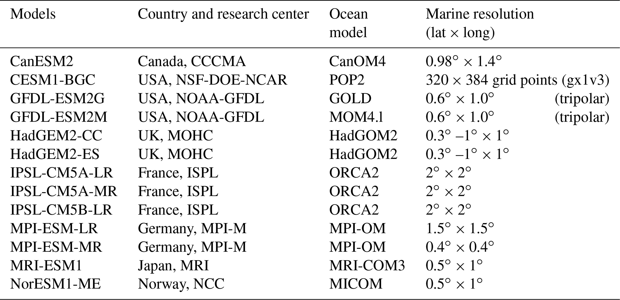
An empirical orthogonal function (EOF) analysis is performed on the standardized winter-average North Atlantic sea level pressure to obtain the first mode (EOF1) of the SLP field, that is, the NAO mode (Hurrell and Deser, 2009). Figure 1 shows the NAO modes of the observation and CMIP5 model simulations. The NAO mode calculated with the observed SLP is significant, which explains 51.8 % of the total variance. The explanation variance of the NAO mode by the models ranges from 27.5 to 56.4 %, and the explanation variance of most models is lower than that of the observation-based result. It is worth noting that the NAO mode simulated by the HadGEM2-CC in 1955–2005 is not statistically significant. The observation shows that the low-pressure action center of the NAO is at around 77.5∘ N, 2.5∘ E, and that the high-pressure action center is around 42.5∘ N, 2.5∘ W (Fig. 1). The CMIP5 models can basically reproduce the NAO mode, although there are some slight differences of the locations of the NAO action centers between different models and between the models and observation. The differences between the NAO patterns simulated by these models with the same external-forcing data are probably induced by their different model structures and values of parameters. In addition, many studies are based on the observation that there is a shift in the action centers of the NAO (Jung et al., 2003; Moore et al., 2013), and this shift is related to the phase of the NAO (Cassou et al., 2004; Jing et al., 2019). The locations of the NAO action centers simulated by most of the 13 CMIP5 models in different NAO phases do not show obvious movements illustrated by the observation (Fig. S1), which means that the climate variations simulated by the models are more symmetrical than the actual situation.
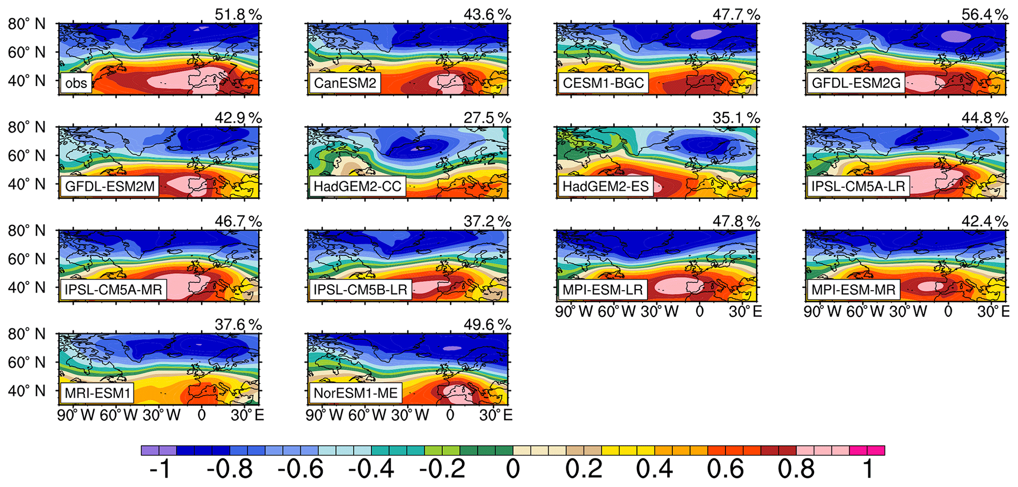
Figure 1EOF1 of observed and simulated standardized winter-average sea level pressure over a particular region of the North Atlantic (30–80∘ N, 100∘ W–40∘ E). The time periods for the observation and models range from 1965 to 2015 and from 1955 to 2005, respectively. The simulated results are based on a historical experiment of CMIP5 (r1i1p1).
The CMIP5 models can basically reproduce the spatial distribution of the SST in the NA (spatial correlation coefficients with the observations are all above 0.99, Fig. S2), although the CMIP5 models underestimate the annual mean SST of the NA (C. Z. Wang et al., 2014). In terms of interannual variability of winter SST in the NA (0–65∘ N) (Fig. 2), all CMIP5 models can reproduce the strong interannual variability of the SST in the Gulf Stream extension, but the simulated strong interannual variability of the SST by most models is more easterly than the observations. With a climate system model, Siqueira and Kirtman (2016) found that the change of ocean component model resolution can change the simulated SST variability, locations of atmospheric circulation anomalies, and air–sea interactions in the North Atlantic. The change is induced by the impact of the resolution on the ocean dynamics, such as ocean fronts and eddies in the Gulf Stream which can be well resolved in the high-resolution model with a horizontal resolution of 0.1∘ × 0.1∘. Nevertheless, the highest horizontal resolution of these ocean component models used in this study is 0.4∘ × 0.4 ∘ (MPI-ESM-MR), and the comparison of MPI-ESM-LR and MPI-ESM-MR, which are both from the same institution but have different ocean component model resolutions, shows that the SST variability in the Gulf Stream is not significantly different. This indicates that the resolution of these models is still not enough to investigate the SST variability in the Gulf Stream and may explain the deviation between the simulated SST variability and the observed one. In addition, some models also simulate strong interannual variability at higher latitudes, which is not observed.
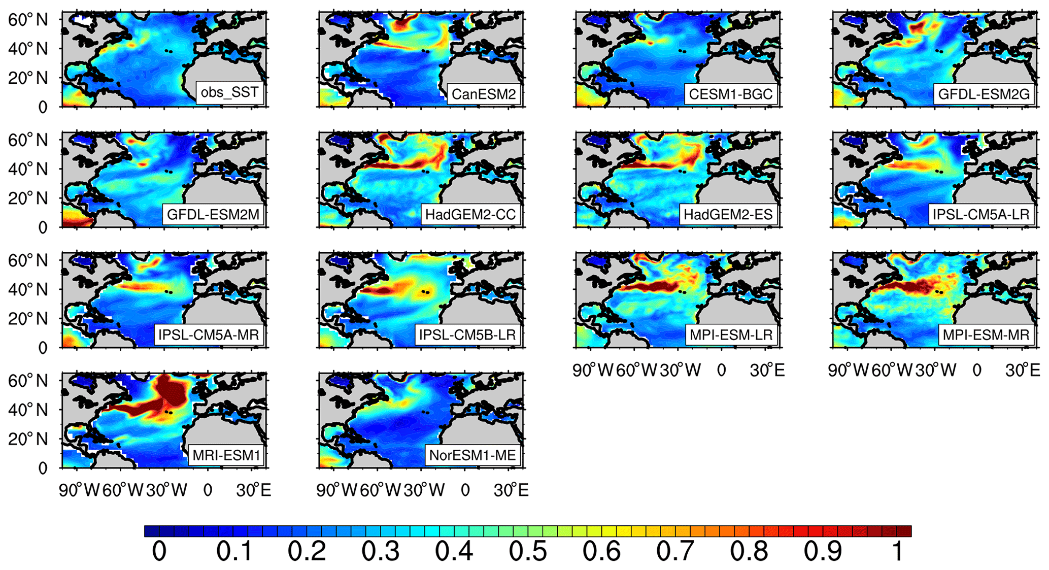
Figure 2Observed and simulated SST interannual variability (∘, 1 SD). The time periods for the observation and models range from 1965 to 2015 and from 1955 to 2005, respectively. The simulated results are based on a historical experiment of CMIP5 (r1i1p1).
3.1.2 Temporal period
Figure 3a shows the periods of the observation-based NAO indices provided by NCAR and model-based NAO indices calculated with the method proposed by Zheng et al. (2013). The power spectra of the NAO indices are also shown in Fig. S3. The significant periods (at a 90 % confidence level) of the observed NAO index are 3, 4.8, and 8–10 years, shown as a red line in Fig. 3a, characterized by interannual and decadal signals. Most models can reproduce significant interannual signals of around 3 years, and CESM1-BGC, GFDL-ESM2M, IPSL-CM5B-LR, MPI-ESM-MR, and NorESM1-ME can reproduce the interannual signal of 4–5 years. It should be noted that HadGEM2-CC without significant EOF1 of SLP does not have a significant interannual period of the NAO index. Therefore, we will not emphasize the analysis of simulated results from HadGEM2-CC in the following content. Compared with the observation, the model bias of the NAO periods is mainly reflected on a decadal scale, which is consistent with the analysis of the CMIP5 models by Wang et al. (2017) based on the annual NAO. Only five models (CanESM2, HadGEM2-CC, IPSL-CM5A-MR MPI-ESM-LR, and MRI-ESM1) can reproduce the decadal signals longer than 8 years, and GFDL-ESM2G can simulate the periods of 16 and 18 years, characterized by decadal signals, which are not observed.
Figure 3Periodicities of the observed and simulated winter-average NAO indices (a) and area-average SST anomalies in the subtropical (b, 25–45∘ N) and subpolar NA (c, 45–65∘ N), determined by power spectrum analysis. The periodicities are determined by calculating the red noise confidence interval and choosing those at the 90 % confidence level. The y coordinate of the horizontal lines or areas is the significant period of observation. The time periods for the observation and models range from 1965 to 2015 and from 1955 to 2005, respectively. The simulated results are based on a historical experiment of CMIP5 (r1i1p1).
Figure 3b and c show the observed and simulated periods of winter area-averaged SST anomalies in the subtropical (25–45∘ N) and subpolar NA (45–65∘ N), respectively. The power spectra of the area-averaged SST anomalies are also shown in Fig. S4 (for the subtropical NA) and S5 (for the subpolar NA). In the subtropical NA, the observed area-averaged SST anomalies have a significant interannual signal of 2 years. Most CMIP5 models can reproduce the 2–4-year interannual signals of SST in this region. Some models, such as HadGEM2-CC/ES and IPSL-CM5A-LR/MR, can simulate the decadal signal of 8–20 years, which is not observed, and some models even produce the multidecadal signal, such as IPSL-CM5B-LR and NorESM1-ME. In the subpolar NA, the observed area-averaged SST anomalies have a significant interannual signal of 3.5 years. There are six models that reproduce a significant period of the area-averaged SST anomalies of about 3.5 years, namely CanESM2, CESM1-BGC, GFDL-ESM2M, IPSL-CM5A-MR, IPSL-CM5B-LR, and MPI-ESM-LR; except for GFDL-ESM2G most models can reproduce the 2-year interannual signal of the SST in the region. Some models – such as CESM1-BGC, GFDL-ESM2G/M, HadGEM2-CC/ES, IPSL-CM5A/B-LR, and MRI-ESM1 – can also simulate the decadal or multidecadal signal of over 8 years, which is not observed.
Based on the above analysis, simulated periods of the NAO indices on an interannual scale are more consistent with the results of observations compared to those on a decadal scale. The observed periods of the area-averaged SST in the subtropical and subpolar NA only present interannual signals. In addition, the impact of the atmospheric anomalies (NAO) on the SST in the NA is mainly reflected in the impact of local change of wind stress on the sea–air heat flux on interannual scales (Eden and Jung, 2001; Chen et al., 2015; Han et al., 2016). Therefore, we will extract the interannual signal of 2–6 years by band-pass filter based on the periods of the NAO and area-averaged SST anomalies to evaluate the relationship between the simulated NAO and SST in the CMIP5 models on an interannual scale.
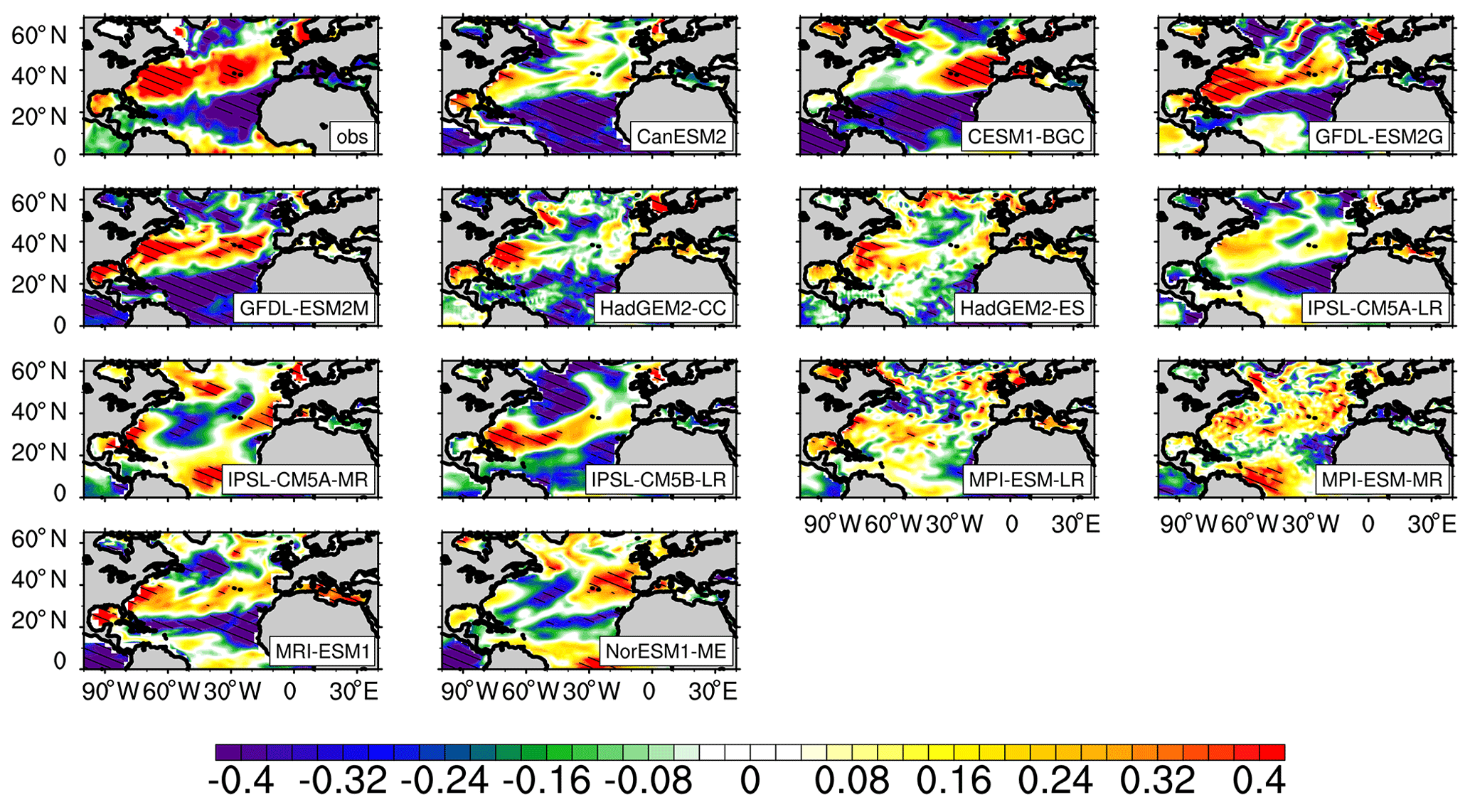
Figure 4Observed and simulated standardized regression coefficients (RCs) of the winter-average SST anomalies against the NAO indices on an interannual scale (with 2–6-year data filtering). Shaded areas indicate that RCs are statistically significant at the 95 % confidence level of Student's t test. The obs is the RCs of observed SST to the NAO indices provided by NCAR. The time periods for the observation and models range from 1965 to 2015 and from 1955 to 2005, respectively. The simulated results are based on a historical experiment of CMIP5 (r1i1p1).
3.2 Responses of NA (0–65∘ N) SST to the NAO
Figure 4 shows the regression coefficients (RCs) of the winter-average SST anomalies against the NAO indices on an interannual scale in the NA (0–65∘ N). The significant RCs between the observed NAO indices and SST anomalies give out a tripole pattern along the meridional direction with positive RCs in the subtropical region (25–45∘ N) and negative RCs in both the tropical (0–25∘ N) and subpolar regions (45–65∘ N), which is consistent with Walter and Graf (2002) and Chen et al. (2015). Compared with the observation, most of the models can roughly reproduce the tripole pattern of the response of the SST anomalies to the NAO. In the region around 20∘ N, all models can reproduce the significant negative response (reaching a 95 % confidence level) east of 40∘ W, and in the subtropical NA 10 models can reproduce significant positive response of the SST anomalies to the NAO near the American coast. The main difference in the RCs between the modeled and observation-based results occurs in the subpolar region, where the simulated locations of the negative-response centers by some of models are different from the observation-based results, especially in CanESM2, HadGEM2-ES, IPSL-CM5A-MR, MPI-ESM-LR/MR, and NorESM1-MR. The simulated and observed factors affecting the response of the SST to the NAO will be compared to explore the reasons for the different response of the SST anomalies to the NAO mainly in subpolar NA.
In HadGEM2-ES, the low-pressure action centers of the NAO are slightly further south than observations (Fig. 1; the low-pressure action center is at around 67.5∘ N), and the negative-response center of the SST to the NAO is also further south than observations. However, in some models (for example IPSL-CM5A-MR and IPSL-CM5B-LR), even if the locations of the low-pressure action center of the NAO are close to that of the observation or even further north, the negative-response center of the SST anomalies related to the NAO is further south than the observation-based results. Therefore, there must be other factors that impact the relationship of the SST and NAO in the subpolar NA in some models.
3.2.1 The role of wind speed
Since the influence of the NAO on the SST is mainly through the wind field in the NA (Zhou et al., 2006; Deser et al., 2010), in order to evaluate the mechanism of the influence of the simulated NAO on the SST in the NA, the response of the wind speed to the NAO should be firstly considered. Figure 5 shows the RCs of the sea surface wind speed anomalies against the NAO indices on an interannual scale, which clearly shows a meridional tripole pattern with negative RCs at middle latitudes (30–40∘ N) and positive RCs at both tropical and high latitudes (north of 40∘ N). This distribution pattern is closely similar to the NAO–SST relationship, which is consistent with the results of Cayan (1992), Marshall (2003), Visbeck et al. (2003), and Deser et al. (2010). All the CMIP5 models can reproduce the impact of the NAO on the sea surface wind field. During the positive phase of the NAO, wind speed is strengthened in the tropical NA and at high latitudes, and weakened at middle latitudes. This is consistent with the fact that during the positive phase of the NAO the deepening of the low pressure in Iceland causes the anomalous east wind superimposed on the midlatitude westerly wind, which weakens the midlatitude wind speed (Deser et al., 2010; Chen et al., 2015). It should be noted that in the subpolar NA the locations of the positive-response center of wind speed anomalies related to the NAO are consistent among different models, which indicates that the difference between the locations of the NAO low-pressure action center simulated by these models has little influence on the locations of the response center of wind speed anomalies related to the NAO.

Figure 5Same as Fig. 4 but for the winter-average sea surface wind speed anomalies against the NAO indices. A missing panel means that the model output is not available.
According to Eqs. (2)–(5), the wind speed anomalies impact the SST by affecting the turbulent heat flux, but the wind speed only affects the magnitude of the turbulent heat flux. Therefore, when analyzing the effect of wind speed anomalies on the turbulent heat flux, it is necessary to consider the direction of the turbulent heat flux, which is determined by the difference of temperature and specific humidity between the atmosphere and the sea surface. From the results of the multiyear-average winter SHF and LHF (Fig. S6), the observed and simulated SHF and LHF are all from the sea to the atmosphere. Considering the directions of the SHF and LHF, the increase in wind speed can significantly increase the turbulent heat flux transported from a large region of the sea surface to the atmosphere.
In order to ensure the accuracy of the observed multiyear-average winter SHF and LHF, three other observation-based SHF and LHF data in winter are selected, and all of these datasets are in the same periods from 1980 to 2015. The distributions of the SHF and LHF from the four reanalysis databases are generally consistent with each other, and the main difference among these datasets is in the intensity of high values, especially in the high-value center of the LHF located in the tropical NA (Fig. 6a). The response of the SHF and LHF anomalies to the NAO in these four datasets is also close to each other, and the main difference among these datasets still occurs in the tropical NA (Fig. 6b). Based on the above analysis, it can be concluded that the difference among the observation-based SHF and LHF does not affect the investigation of the relationship of the SHF and LHF and the NAO and SST in this study because the regions of concern are mainly the subtropical and subpolar NA. In the following text, unless otherwise specified, the observation-based SHF and LHF are the data from the NOAA-CIRES 20th Century Reanalysis version 2.
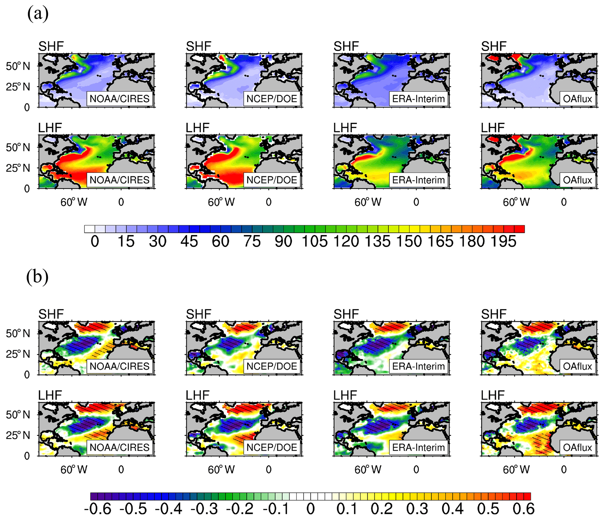
Figure 6(a) Observed multiyear mean winter sensible (SHF) and latent heat flux (LHF) (Wm−2), and (b) standardized RCs of the winter-average SHF and LHF anomalies against the NAO indices. The time periods of the four datasets used in this figure range from 1980 to 2015. The three observation-based data from the NOAA-CIRES (NOAA-CIRES), NCEP (NCEP-DOE), and ECWMF (ERA-Interim) are reanalysis data, and the last one (OAflux) is the optimal syntheses of voluntary observing ships, reanalysis, and satellite data sources.
Most models seem to reproduce the maximum SHF in the Labrador Sea and a large SHF in the Gulf Stream Basin (Fig. S6), and the observed distributions of the LHF are also well reproduced in these models, except that some models, such as CanESM2 and IPSL-CM5B-LR, underestimate LHF in the subpolar NA (Fig. S6). However, there is no evidence that the simulation bias of the magnitude of the multiyear-average LHF can affect the relationship between the NAO and SST anomalies.
Figure 7 shows the RCs of winter turbulent heat flux anomalies against the NAO indices. The significant observed RCs between the NAO indices and the SHF and LHF anomalies in the NA (0–65∘ N) indicate a meridional tripole pattern with negative RCs in the subtropical region and positive RCs in both the tropical and subpolar regions. The simulated and observed locations of the positive RCs in the subpolar region are almost same, which further illustrates that the bias in CMIP5 models regarding the location of the NAO low-pressure action center may have little influence on the NAO–SST relationship. The spatial distribution of the observed RCs is consistent with the results of Eden and Jung (2001) and Deser et al. (2010), and is generally consistent with the meridional distribution of the observed RCs of the sea surface wind speed anomalies against the NAO, from which we can infer that the wind speed anomalies related to the NAO can impact the SHF and LHF anomalies. During the positive phase of the NAO, the increase of wind speed in the tropical and subpolar NA strengthens the turbulent heat flux transported from the ocean to the atmosphere, while the weakening of the wind speed in the subtropical NA weakens the turbulent heat flux. The CMIP5 models can basically reproduce the significant RCs of turbulent heat flux anomalies against the NAO, for which the meridional distribution pattern is the same as the RCs of the wind speed anomalies against the NAO indices.
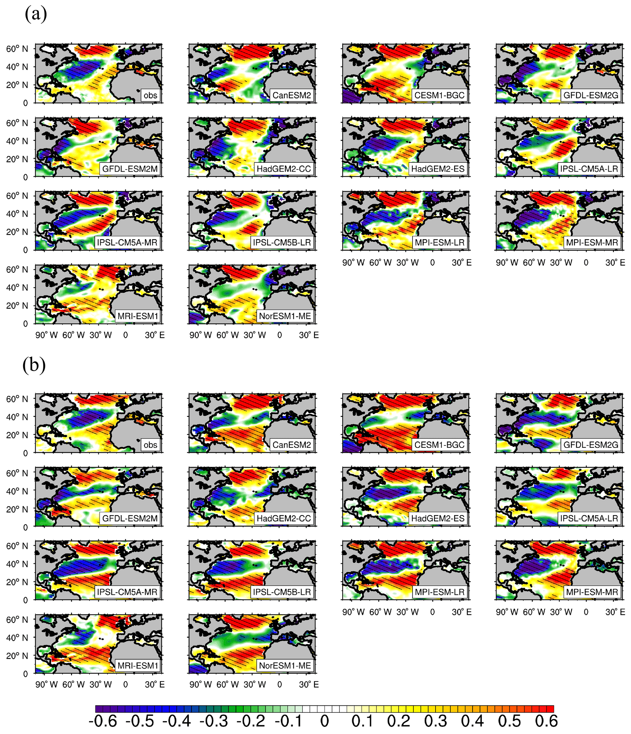
Figure 7Same as Fig. 4 but for the winter-average SHF (a) and LHF (b) anomalies against the NAO indices.
3.2.2 The role of SHF
The variability of the SHF and SST is related. According to the calculation formula of the SST and SHF, the increase of the SHF can decrease SST (Eqs. 2–3), while the decreased SST can further decrease the SHF (Eq. 4). Therefore, when the variations of the SST and SHF are negatively correlated, it can be inferred that the change of the SHF influences the SST, which means that the atmosphere forces the ocean; when the variations of the SST and SHF are positively correlated, the change of the SST leads to the change of SHF, which means that the ocean forces the atmosphere.
Figure 8a shows the observation-based and simulated RCs of the winter-average SST anomalies to the NAO-driven SHF anomalies obtained by the linear regression of the SHF against the NAO indices. As expected, the observed winter-average SST anomalies show significant negative RCs against the observed NAO-driven SHF anomalies in the high-value centers of RCs (absolute value) of the SST anomalies against the NAO index, except for a little region in the eastern NA around 20∘ N where the RCs of SST against the NAO-driven SHF is positive, which is consistent with the RCs of SHF and SST anomalies against the NAO index being negative in this region (Figs. 7a and 4). This indicates that the response of the SST to the NAO is really related to the response of the SST to the NAO-driven SHF, and the atmosphere forces most regions of the North Atlantic Ocean in winter. Considering the significant relationship between the SST, SHF, and wind speed anomalies and the NAO, it can be concluded that in winter the NAO can impact the SST by affecting the SHF in most regions of the NA through the change of wind speed. There are some differences between the modeled and observed relationships of the SST and SHF. In the subtropical NA, there are no significant negative-response centers of the SST anomalies related to the NAO-driven SHF anomalies near the American coast in CESM1-BGC, IPSL-CM5A-LR, and NorESM1-ME, so the three models cannot simulate positive-response centers of the SST anomalies related to the NAO. The significant positive response of the SST anomalies to the NAO-driven SHF in the subtropical NA of IPSL-CM5A-MR and NorESM1-ME also induces a significant negative response of the SST anomalies to the NAO. In the subpolar NA, the locations and magnitude of negative-response centers of the SST anomalies related to the NAO-driven SHF anomalies in some models are not consistent with the observation-based results, but they are consistent with those of the SST anomalies related to the NAO by all CMIP5 models. This can partly explain why the negative-response center of SST anomalies related to the NAO in the subpolar NA in some models are inconsistent with the observation.
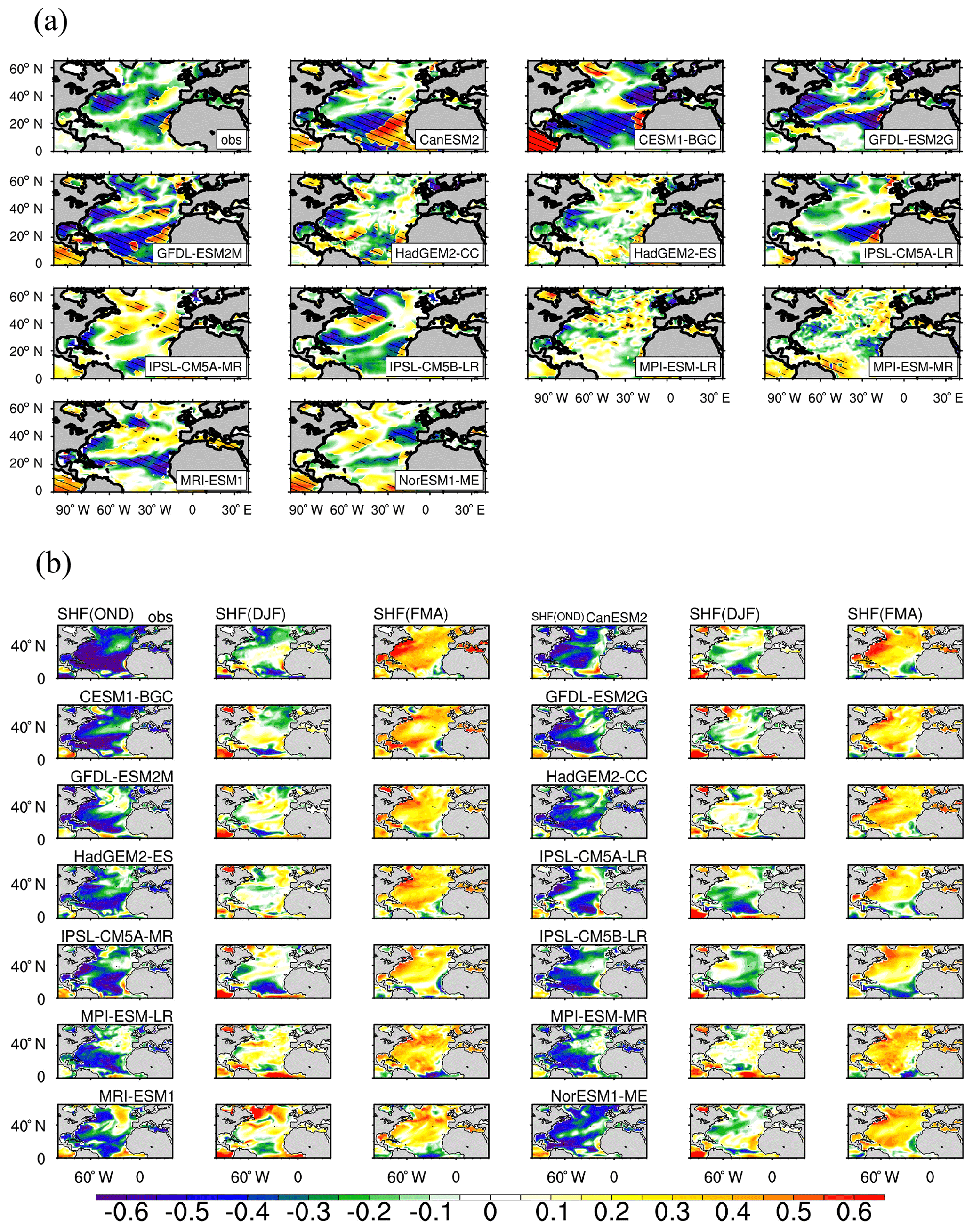
Figure 8(a) Same as Fig. 4 but for the winter-average SST anomalies against the NAO-driven SHF anomalies. (b) The standardized lagged (lead) covariance between monthly SHF anomalies from October to December and from February to April with the SST anomalies from December to January. OND refers to the SHF from October to December, and FMA refers to the SHF from February to April.
There may be two reasons for the models' bias regarding the locations and magnitude of negative-response centers of the winter-average SST anomalies related to the NAO-driven SHF anomalies: the areas where air–sea interaction is dominated by the atmosphere are different from the observation, and there may be other factors which play a dominate role in the variation of the SST and further impact the relationship between the anomalies of the SST and SHF. To investigate the reason, lagged (lead) covariance analysis of monthly anomalies of the SHF and SST is used and shown in Fig. 8b. The lagged or lead time is 2 months. Here, the monthly SHF anomalies from October to April and monthly SST anomalies from December to February of the same year are used. When the observed SST anomalies lag (lead) SHF anomalies by 2 months, the covariance between the SHF and SST anomalies is negative (positive) in most regions. When the change of SHF synchronizes with the change of SST, the covariance between the anomalies of the SHF and the SST is negative in the subpolar and western subtropical NA, which means that the forcing from the SHF (atmosphere) to the SST (ocean) is still dominated in the interaction between the SHF and SST in these regions.
When the SST anomalies lag the SHF anomalies by 2 months, all CMIP5 models can reproduce the negative covariance between SHF and SST anomalies in most regions of the NA, although there are some models that simulate weak positive covariance in some regions of the subpolar NA, such as GFDL-ESM2M, HadGEM2-CC/ES, IPSL-CM5A-L/MR, MPI-ESM-LR, and MRI-ESM1, indicating that other factors (such as the internal motion of ocean) have an impact on the variations of the SST in the regions beyond the SHF in these models. When the change of SHF is synchronized with the change of the SST, most models reproduce the weakening of the SHF's influence on the SST, especially in the subtropical and tropical NA, and in the six models mentioned above the geographical range of the negative covariance in the subpolar NA is still smaller than that of the observed data, especially in MRI-ESM1. It is worth mentioning that the locations of the covariance center simulated by most models in the subpolar NA are consistent with that of the RCs of the winter-average SST anomalies against the NAO-driven SHF anomalies and that of the winter-average SST anomalies against the NAO, while in some models, such as MRI-ESM1 and NorESM1-ME, the performance of simulating the covariance of the SHF and the SST is not consistent with that of simulating the response of the SST to the NAO-driven SHF. In MRI-ESM1, the covariance of the SHF and the SST in the subpolar NA deviates from the observation-based results, while the response of the SST to the NAO-driven SHF and NAO is close to the observation results. In NorESM1-ME, the covariance of the SHF and the SST is close to the observation-based results in the subpolar NA, while the response of the SST to the NAO-driven SHF and NAO is biased in this region. This demonstrates that in some models there are other factors that can influence the relationship of the NAO-driven SHF and NAO and the SST in the subpolar NA.
3.2.3 The role of LHF
The LHF is calculated by wind speed and the difference between the saturation specific humidity of lower air and the sea surface. Because the saturation specific humidity of sea surface is a function of the SST (Eq. 6), according to the calculation formulas of the SST and LHF (Eqs. 2, 3, 5, and 6), the relationship between the LHF and SST is similar to the one between the SHF and SST. This means that, when the variations of the SST and LHF are negatively correlated, the atmosphere forces the ocean through the LHF and that, when the variations of the SST and LHF are positively correlated, the ocean forces the atmosphere.
Figure 9a shows the RCs of the observed and simulated winter-average SST anomalies against the NAO-driven LHF anomalies. The distributions of the RCs are similar to those of the SST anomalies against NAO-driven SHF anomalies in a large area of the NA. The main difference between the response of the SST to the SHF and to the LHF is that the observed and modeled positive RCs of the SST anomalies against NAO-driven SHF anomalies in the eastern NA around 20∘ N do not occur in the regression of the SST anomalies against NAO-driven LHF anomalies. This indicates that the influence of the LHF on the SST probably controls the RCs of the SST anomalies against the NAO in this region. The observed difference between the relationship of the SST and NAO-driven SHF and that of SST and NAO-driven LHF is well reproduced by most models, and the main bias of the simulated response of the SST to the NAO-driven LHF is also close to that to the NAO-driven SHF. In each model the locations and magnitude of the negative-response centers of the SST anomalies related to the NAO-driven LHF anomalies in the subpolar NA are very similar to those to the NAO-driven SHF anomalies. Therefore, the biases of the relationship between the SST anomalies and NAO-driven SHF and LHF anomalies together lead to the bias of the locations and magnitude of the negative-response center of the SST anomalies related to the NAO in the subpolar NA in these models.
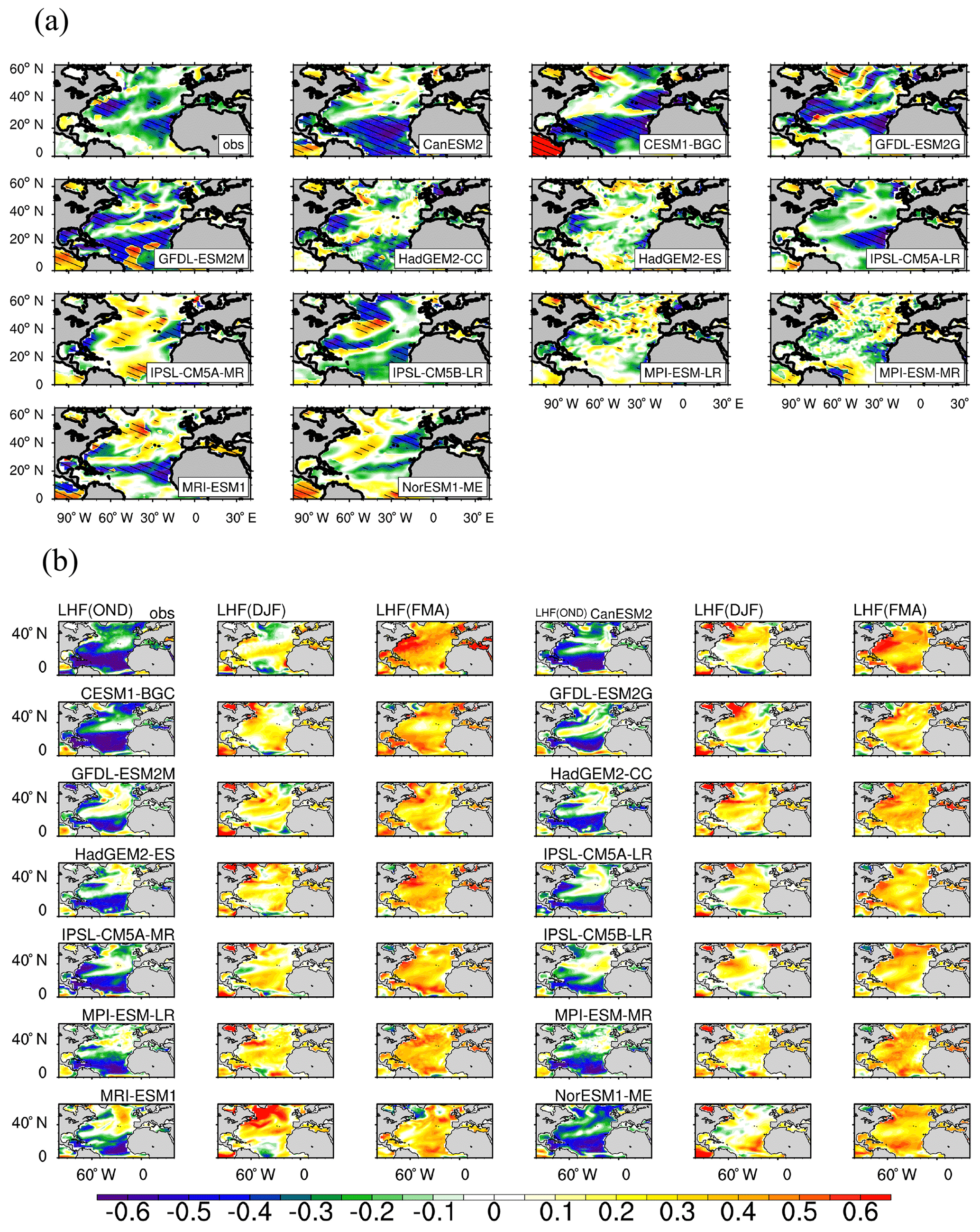
Figure 9Same as Fig. 8 but for the LHF.
Figure 9b shows the lagged (lead) covariance between the anomalies of the LHF and SST. As well as the relationship of the SST and SHF, when the observed SST anomalies lag (lead) those of the LHF by 2 months, there is an obviously negative (positive) covariance in a large region of the NA, which indicates that the change of LHF (SST) can influence the change of SST (LHF) after 2 months. It should be noted that, whether the change of the LHF is ahead of or synchronized with the SST, the geographical ranges and magnitudes of the negative covariance of LHF and SST are smaller than those of the SHF and SST. For example, when the changes of the SST and LHF are synchronized, there is an obviously positive covariance in the subtropical NA, which has a larger value and a greater range than that of the synchronized SHF anomalies and SST anomalies. This demonstrates that the timescale of the LHF affecting SST is shorter than that of the SHF affecting SST, and the ocean plays an important role in the interaction of LHF and SST in a large region of the NA. The CMIP5 models basically reproduce the lagged or lead relationship between the SST anomalies and the LHF anomalies. When the SST anomalies lag the LHF anomalies, most models – except for CanESM2, CESM1-BGC, and NorESM1-ME – simulate a large region of positive covariance in the subpolar NA, which only occurs in a small region in the observation-based results. When the two variables in the models are synchronized, the range and magnitude of positive covariance simulated by models are significantly larger than those in the observation-based results. It can be concluded that the oceanic forcing on the atmosphere through the LHF variation is enhanced in the models, which results in a positive response of the winter-average SST anomalies to the LHF anomalies in the NA, which weakens the magnitude of the negative-response center of the SST anomalies related to the NAO and may be the reason for the bias of NorESM1-ME, which has a realistic relationship of the SHF and SST, regarding the response of the SST anomalies to the NAO in the subpolar NA.
We evaluated the influence mechanism of the NAO on the SST in the NA (0–65∘ N) simulated by the 13 models of CMIP5. In most of the models, the significant periods of interannual signals obtained by the power spectra are consistent with the observation-based results, and the significant periods of the subpolar and subtropical area-averaged SST in the observation are mainly characterized by interannual signals, so we mainly evaluated the simulation of the relationship between the winter-average SST and NAO by these 13 CMIP5 models on an interannual scale.
Based on the observations, the RCs of winter-average SST anomalies against the NAO show a significant tripolar distribution in the meridional direction in the NA. Most of the models can reproduce the tripole pattern of the response of the SST anomalies to the NAO. In the subtropical NA (25–45∘ N), most models can reproduce the significant positive-response center near the American coast. However, in the subpolar region, the simulated locations and magnitude of the negative-response centers by most models have some difference from the observation.
Further evaluation of the response of the winter-average SST anomalies to the NAO simulated by the 13 CMIP5 models in the NA shows that the models can basically reproduce the impact of the wind speed anomalies related to the NAO on turbulent heat flux anomalies in the NA, but the relationship between the anomalies of the NAO-driven turbulent heat flux and SST simulated by the models has some differences from observation-based results in some regions of the NA, especially in the region north of 45∘ N. In the subpolar NA, the geographical range and magnitude of the negative response of the SST anomalies to the NAO-driven SHF and LHF simulated by most of the models are smaller than those in the observation-based results, which may lead to the bias of the locations and magnitude of the negative-response centers of the SST anomalies related to the NAO. One piece of evidence for this conclusion is that the bias of locations of negative-response centers of the SST anomalies related to the NAO-driven SHF and LHF simulated by most models corresponds to the bias of locations of negative-response centers of the SST anomalies related to the NAO. It seems that the influence of the LHF on the SST is weaker than that of the SHF on the SST in most regions from both the observation-based and simulated results of most models, except for the eastern tropical NA and NorESM1-ME. The weak negative response or strong positive response of the SST anomalies to the NAO-driven LHF simulated by most models may be caused by the rapid response of the ocean to the change of the LHF.
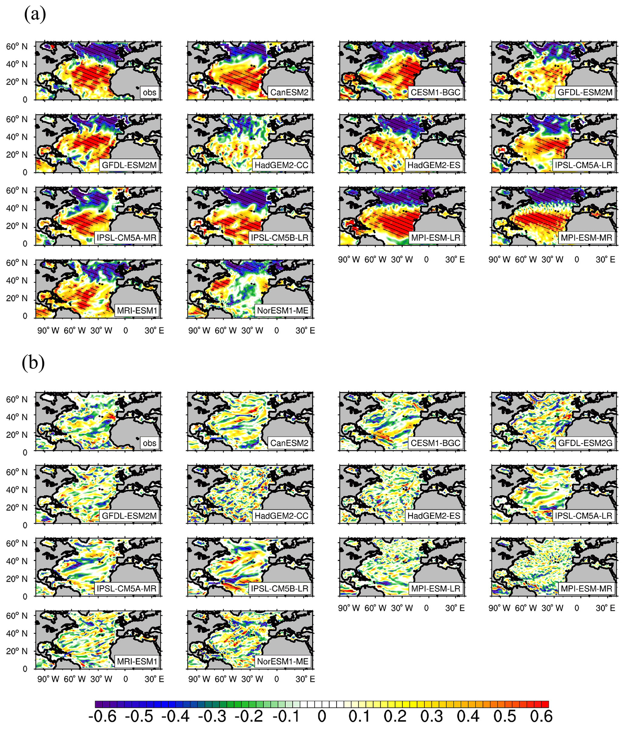
Figure 10(a) Observed and simulated standardized RCs of the winter-average sea surface meridional velocity anomalies against the NAO index. (b) Standardized correlation coefficients between the winter-average SST anomalies and the change in SST caused by NAO-driven surface meridional velocity on an interannual scale (with 2–6-year data filtering, Eqs. 7–9). Shaded areas indicate that the correlation coefficients are statistically significant at the 95 % confidence level of Student's t test. The obs is the observation-based result. The time periods for the observation and models range from 1981 to 2015 and from 1955 to 2005, respectively. The simulated results are based on a historical experiment of CMIP5 (r1i1p1).
Although the response of the SST anomalies to the NAO in most models can be explained by the bias of the SST response to the air–sea turbulent heat flux, there are still some models whose performance has not been reasonably explained, for example MRI-ESM1, in which the relationship of the SST and the NAO-driven heat flux is not consistent with the observation-based result at high latitudes, but the response of the SST to the NAO is realistic. There may be some other factors which can affect the relationship of the SST and NAO, or deficiencies in the method used in this study.
5.1 Heat advection transport
In addition to the turbulent heat flux, the changes of long- and short-wave radiation and the ocean circulation also have effects on the change of the SST. The long-wave radiation on the sea surface is mainly determined by SST, while the change of short-wave radiation does not have a strong relationship with the NAO (the figure is omitted). The simulated relationship between the SST and the NAO by the CMIP5 models may be also related to the NAO-driven horizontal heat advection, although some other studies have argued that the impact of ocean heat advection on the change of SST in the subtropical NA is mainly on a decadal scale (Delworth and Mehta, 1998; Krahmann et al., 2001).
From the observation-based RCs of vo anomalies against the NAO in winter (Fig. 10a), it can be seen that on an interannual scale in the subtropical NA the observed vo (positive values indicate northward) anomalies have a significant positive response to the NAO, and in the subpolar NA they have a significant negative response to the NAO. The observed and simulated correlation coefficients between the winter-average SST anomalies and the SST variations caused by NAO-driven vo on an interannual scale, which are calculated with Eqs. (7) and (8), are shown in Fig. 10b. There seems no obvious regular distribution of the influence of the NAO-driven vo on the SST which can be related to the tripole pattern of the response of the SST anomalies to the NAO (Fig. 10b), so on an interannual timescale the role of the heat advection to the change of the SST in the NA can be ignored.
5.2 Band-pass filter
Cane et al. (2017) point out that the low-pass filter can influence the correlations of the SST and heat flux. Therefore, the influence of the band-pass filter should be analyzed. We also did regression analysis of unfiltered winter-average SST anomalies and NAO indices (Fig. S7). It is found that, except for the models of IPSL-CM5A-MR and MPI-ESM-L/MR, there is no obvious difference in the distribution of standardized RCs of the SST and NAO between the filtered and unfiltered results, and the main difference is that the RCs from the unfiltered data are slightly smaller than those from the filtered data in the subtropical NA (Fig. 4) of both the observation-based results and the majority of the modeled results. In IPSL-CM5A-MR and MPI-ESM-L/MR, both the magnitude and location of the significant positive RCs of the unfiltered SST and NAO indices in the subtropical NA are changed and are much closer to the observation-based results than those of the filtered results. This indicates that in these three models the signals over 8 years probably play a more important role in the response of the SST to the NAO. It should be noted that in the tropical and subpolar NA the RCs of the SST against the NAO in the unfiltered observation-based results are enhanced, but those in most of the unfiltered modeled results are weakened. The area of the negative response of the SST to the NAO is enlarged in the unfiltered results of NorESM1-ME and much closer to the observation-based results than that in the filtered results. The periods of the NAO and SST illustrated in Fig. 3 do not provide us with enough information to explain the phenomenon occurring in the observation-based results and simulated results of NorESM1-ME, but they do indicate that the data filtering process can affect our evaluation of individual models to some extent. For the relationship between the SST and NAO-driven SHF and LHF (Fig. S8), the magnitude of the RCs of the SST and NAO-driven SHF and LHF anomalies is enhanced in the unfiltered observation-based results but weakened in most of the unfiltered model results, except for the subtropical NA of IPSL-CM5A-MR and MPI-ESM-L/MR and the subpolar NA of NorESM1-ME. The difference between the unfiltered and filtered RCs of the SST and the NAO-driven SHF and LHF anomalies in the models is consistent with that between the unfiltered and filtered RCs of the SST and NAO. Once again, the NAO-driven heat flux anomalies are the key to controlling the response of the SST to the NAO.
The periods of NAO indices are sensitive to the time period analyzed. The significant periods of the observed NAO index in 1897–2005 are 2.3–2.7, 4.7–5.8, and 8.3 years, but in 1955–2005 they become 3, 4.8, and 8–10. The periods of NAO indices are also sensitive to the dataset, which is analyzed in Jing et al. (2019). Therefore, the influence of the cutoff period used in the filter should be analyzed. We do regression analysis of winter-average SST anomalies and NAO indices on an interannual scale calculated by 2–4-year filtering (Fig. S9) and find that the observed and simulated patterns of the response of the SST anomalies to the NAO based on 2–4-year filtering is close to the results based on 2–6 years, but the intensity of the response of the SST anomalies to the NAO in the observation and most models is strengthened. It should be noted that with the 2–4-year filtering the performance of the response of the SST to the NAO in MPI-ESM-L/MR and NorES1-ME is very close to that with the 2–6-year filtering. Combining the difference between the unfiltered and filtered results, it can be concluded that there are indeed signals on a long timescale which have a more important influence on the relationship of the SST and NAO, although we cannot get supporting information from the analysis of periodicity.
5.3 NAO index definition
Currently, there are many NAO index definitions; because the method used to define NAO index differs, the description of several associated phenomena will also vary (Pokorná and Huth, 2015). In addition to the site-based NAO index provided by NCAR in this study, the two other observation-based NAO indices defined by the method of Gong and Wang (2000) and the method used to calculate model NAO indices (Zheng et al., 2013) are applied to study the relationship between different NAO indices and SST on an interannual scale (Fig. S10). The NAO index defined by different methods does affect the relationship between the NAO and SST in the tropical NA but has only little effects on the relationship in both the subpolar and subtropical NA. This suggests that, if one focuses on the relationship of the SST and NAO in the tropical NA, one should be careful of his choice of the NAO indices.
5.4 Initial fields and external forcing for models
Kay et al. (2015) did ensemble experiments by adding different minute perturbations to the atmosphere as initial conditions to study the internal variability. There are also some historical ensemble experiments in CMIP5 which are initialized with different initial conditions in 1850. The initial conditions of these ensemble members are from the different integration times of the piControl experiments, so these initial conditions represent the different time histories of internal variability. The relationship of the NAO and SST simulated by the models with differing initial fields (r1i1p1 and r3i1p1), as previously discussed, are compared (Fig. S11). Seven of the 13 models employed the historical experiment results with different initial fields. The locations of the response centers of the SST anomalies related to the NAO simulated by six of the seven models in the r3i1p1 experiments are close to those from the r1i1p1 experiments (Fig. S11), while the magnitude of the response centers simulated in the r3i1p1 experiments is stronger than that in the r1i1p1 experiments (Fig. 4). The locations and magnitude of response centers of the SST anomalies related to the NAO simulated by MPI-ESM-MR in the r3i1p1 experiment are obviously different from those in the r1i1p1 experiment with the same filtering cutoffs, and are closer to the observation and the 2–4-year filtering results of the r1i1p1 experiment. The significant periods of the NAO in the experiments of r3i1p1 are also different from those of r1i1p1 (Fig. S12), but there is no obvious law about the significant periods and the magnitude of the response of the SST to the NAO in these seven models. We cannot figure out the reason for the difference between these two sets of experiments, especially in MPI-ESM-MR, but it should be emphasized that the influence of the initial conditions on the result needs to be considered in the evaluation of some individual models.
Besides the initial fields, the external forcing may impact the relationship of the SST and the NAO in models. To investigate the influence of the external-forcing data of the historical experiments, the outputs from the piControl experiments are used to compare with those from the historical experiments. The relationships of the NAO and SST from the piControl experiments of the 13 CMIP5 models are analyzed (Fig. S13). The locations of the response centers of the SST related to the NAO are close to those in historical experiments of most models (except for the subtropical NA of CESM1-BGC). The main difference between the piControl and historical experiments is the magnitude of the response of the SST to the NAO, which also occurs in the difference between the two sets of historical experiments (r1i1pi1 and r3i1p1). It should be noted that the result of the piControl experiment in MPI-ESM-MR is very similar to its r3i1p1 historical experiment but is different from its r1i1p1 historical experiment. The response of the SHF and LHF to the NAO in the piControl experiments (Fig. S14) is also stronger than that in the r1i1p1 historical experiments (Fig. 7). Based on the above analysis, it can be concluded that there is less influence of the external forcing on the NAO–SST relationship in most models, especially on the locations of response centers, but in some individual models the influence of external forcing cannot be ignored. Some studies have shown that in the climate models the amplitude of the response to the external forcing (such as volcanic forcing, solar variability, and ozone depletion) is weak, which leads to weak predictable signals in these models, although these models can predict observed climate variability (Scaife and Smith et al., 2018). The weak predictable signals inhibit the estimation of forced climate variability in the Atlantic sector (Scaife and Smith et al., 2018). The weak influence of the external forcing on the NAO–SST relationship was also found in the CMIP5 models in this work. Smith et al. (2020) have argued that a large ensemble number can overcome the signal-to-noise paradox, which probably provides a reference for the future application of CMIP models in the predications.
The URLs from which to download all data used in this study are described in Sect. 2.1. All data for results are available by contacting the corresponding author.
The supplement related to this article is available online at: https://doi.org/10.5194/os-16-1509-2020-supplement.
YJ, YL, and YX designed the research. YJ analyzed the data under the guidance of YCL and YX, and prepared the manuscript with contributions from YL and YX.
The authors declare that they have no conflict of interest.
All the authors thank the National Center for Atmospheric Research for providing the sea level pressure data; the Hadley Centre Global Sea Ice and Sea Surface Temperature (HadiSST) for providing sea surface temperature data; and the National Oceanic and the Atmospheric Administration (NOAA) for providing the 10 m wind speed, turbulent heat flux, and seawater meridional velocity data. The authors thank the institutions that developed the CMIP5 Earth system models and provided simulation results. Finally, the authors also thank the reviewers and topical editor for their conscientious reviews and useful comments on an earlier version of this paper.
This work was supported jointly by the National Key Research and Development Program of China (no. 2016YFB0200800), the National Natural Science Foundation of China (grant no. 41530426), and the Strategic Priority Research Program of the Chinese Academy of Sciences (grant no. XDB42000000).
This paper was edited by Matthew Hecht and reviewed by two anonymous referees.
Behringer, D. W. and Xue, Y.: Evaluation of the global ocean data assimilation system at NCEP: The Pacific Ocean, Proc. Eighth Symp. on integrated observing and assimilation systems for atmosphere, oceans, and land surface, AMS 84th annual meeting in Washington State Convention and Trade Center, Seattle, Washington, 11–15 January 2004, Am. Meteorol. Soc., 2004.
Bellucci, A. and Richards, K. J.: Effects of NAO variability on the North Atlantic Ocean circulation, Geophys. Res. Lett., 33, L02612, https://doi.org/10.1029/2005gl024890, 2006.
Bretherton, C. S., Widmann, M., Dymnikov, V. P., Wallace, J. M., and Bladé, I.: The effective number of spatial degrees of freedom of a time-varying field, J. Clim., 12, 1990–2009, 1999
Buckley, M. W. and Marshall, J.: Observations, inferences, and mechanisms of the Atlantic Meridional Overturning Circulation: A Review, Rev. Geophys., 54, 5–63, https://doi.org/10.1002/2015RG000493, 2016.
Cane, M. A., Clement, A. C., Murphy, L. N., and Bellomo, K.: Low pass filtering, heat flux and Atlantic Multidecadal Variability, J. Clim., 30, 7529–7553, https://doi.org/10.1175/JCLI-D-16-0810.1, 2017.
Cassou, C., Terray, L., Hurrell, J. W., and Deser. C.: North Atlantic winter climate regimes: spatial asymmetry, stationarity with time, and oceanic forcing, J. Clim., 17, 1055–1068, 2004.
Cayan, D. R.: Latent and sensible heat flux anomalies over the northern oceans: driving the sea surface temperature, J. Phys. Oceanogr., 22, 859–881, 1992.
Chen, H., Schneider, E. K., and Wu, Z.: Mechanisms of internally generated decadal-to-multidecadal variability of SST in the Atlantic Ocean in a coupled GCM, Clim. Dynam., 46, 1–30, https://doi.org/10.1007/s00382-015-2660-8, 2015.
Compo, G. P., Whitaker, J.S., Sardeshmukh, P. D., Matsui, N., Allan, R. J., Yin, X., Gleason, B. E., Vose, R. S., Rutledge, G., Bessemoulin, P., Brönnimann, S., Brunet, M., Crouthamel, R. I., Grant, A. N., Groisman, P.Y., Jones, P. D., Kruk, M., Kruger, A. C., Marshall, G .J., Maugeri, M., Mok, H. Y., Nordli, Ø., Ross, T. F., Trigo, R. M., Wang, X. L., Woodruff, S. D., and Worley, S. J.: The Twentieth Century Reanalysis Project, Q. J. Roy. Meteor. Soc., 137, 1–28, https://doi.org/10.1002/qj.776, 2011.
Czaja, A. and Frankignoul, C.: Observed impact of Atlantic SST anomalies on the North Atlantic oscillation, J. Clim., 15, 606–623, 2002.
Dee, D. P., Uppala, S. M., Simmons, A. J., Berrisford, P., Poli, P., Kobayashi, S.,Andrae, U., Balmaseda, M. A., Balsamo G., Bauer P., Bechtold P., Beljaars, A. C. M., Berg, L. V., Bidlot, J., Bormann, N., Delsol, C., Dragani, R., Fuentes, M., Geer, A. J. Haimberger, L., Healy, S. B., Hersbach, H., Hólm, E. V., Isaksen, L., Kållberg, P., Köhler, M., Matricardi, M., McNally, A. P., Monge‐Sanz, B. M., Morcrette, J. J., Park, B. K., Peubey, C., Rosnay, P. D., Tavolato, C., Thépaut, J. N., and Vitart, F.: The ERA-Interim reanalysis: Configuration and performance of the data assimilation system, Q. J. Roy. Meteor. Soc., 137, 553–597, https://doi.org/10.1002/qj.828, 2011.
Delworth, T. L. and Mehta, V. M.: Simulated interannual to decadal variability in the tropical and sub-tropical North Atlantic, Geophys. Res. Lett., 25, 2825–2828, https://doi.org/10.1029/98gl02188, 1998.
Delworth, T. L., Zeng, F. R., Zhang, L. P., Zhang, R., Vecchi, G. A., and Yang, X. S.: The central role of ocean dynamics in connecting the North Atlantic Oscillation to the extratropical component of the Atlantic Multidecadal Oscillation, J. Clim., 30, 3789–3805, 2017.
Deser, C., Alexander, M. A., Xie, S. P., and Phillips, A. S.: Sea surface temperature variability: patterns and mechanisms, Annu. Rev. Mar. Sci., 2, 115–143, https://doi.org/10.1146/annurev-marine-120408-151453, 2010.
Eden, C. and Jung, T.: North Atlantic interdecadal variability: oceanic response to the North Atlantic Oscillation (1865–1997), J. Clim., 14, 676–691, 2001.
Flatau, M. K., Talley, L., and Niiler, P. P.: The North Atlantic Oscillation, surface current velocities, and SST changes in the subpolar North Atlantic, J. Clim., 16, 2355–2369, https://doi.org/10.1175/2787.1, 2003.
Gastineau, G., D'Andrea, F., and Frankignoul, C.: Atmospheric response to the North Atlantic Ocean variability on seasonal to decadal time scales, Clim. Dynam., 40, 2311–2330, https://doi.org/10.1007/s00382-012-1333-0, 2012.
Gong, D. Y. and Wang, S. W.: The North Atlantic Oscillation index and its interdecadal variability, Chin. J. Atmos. Sci., 24, 187–192, https://doi.org/10.3878/j.issn.1006-9895.2000.02.07, 2000.
Han, Z., Luo, F. F., and Wan, J. H.: The observational influence of the North Atlantic SST tripole on the early spring atmospheric circulation, Geophys. Res. Lett., 43, 2998–3003, https://doi.org/10.1002/2016GL068099, 2016.
Hurrell, J. W. and Deser C.: North Atlantic climate variability: the role of the North Atlantic Oscillation, J. Mar. Syst., 79, 231–244, https://doi.org/10.1016/j.jmarsys.2009.11.002, 2009.
Jing, Y., Li, Y. C., Xu, Y. F., and Fan, G. Z.: Influences of different definitions of the winter NAO index on NAO action centers and its relationship with SST, Atmos. Ocean. Sci. Lett., 12, 320–328, https://doi.org/10.1080/16742834.2019.1628607, 2019.
Jung, T., Hilmer, M., Ruprecht, E., Kleppek, S., Gulev, S. K., and Zolina, O.: Characteristics of the recent eastward shift of interannual NAO variability, J. Clim., 16, 3371–3382, 2003.
Kalnay, E., Kanamitsu, M., Kistler, R., Collins, W., Deaven, D., Gandin, L., Iredell, M., Saha, S., White, G., Woollen, J., Zhu, Y., Chelliah, M., Ebisuzaki, W., Higgins, W., Janowiak, J., Mo, K. C., Ropelewski, C., Wang, J., Leetmaa, A., Reynolds, R., Jenne, R., and Joseph, D.: The NCEP/NCAR 40-year reanalysis project, Bull. Am. Meteorol. Soc., 77, 437–470, 1996.
Kanamitsu, M., Ebisuzaki, W., Woollen, J., Yang, S. K., Hnilo, J. J., Fiorino, M., and Potter, G. L.: NCEP–DOE AMIP-II reanalysis (R-2), B. Am. Meteor. Soc., 83, 1631–1643, https://doi.org/10.1175/BAMS-83-11-1631, 2002.
Kay, J. E., Deser C., Phillips, A., Mai, A., Hannay, C., Strand, G., Arblaster, J. M., Bates, S. C., Danabasoglu, G., Edwards, J., Holland, M., Kushner, P., Lamarque J. F. Lawrence, D., Lindsy, K., Middleton, A., Munoz, E., Neale, R., Oleson, K. Polvani, L., and Vertenstein, M.: The Community Earth System Model (CESM) Large Ensemble Project: A Community Resource for Studying Climate Change in the Presence of Internal Climate Variability, Bull. Am. Meteorol. Soc., 96, 1333–49, https://doi.org/10.1175/BAMS-D-13-00255.1, 2015.
Krahmann, G., Vsbeck, M., and Reverdin, G.: Formation and propagation of temperature anomalies along the North Atlantic Current, J. Phys. Oceanogr., 31, 1287–1303, 2001.
Liu, H. L., Wang, C. Z., Lee, S. K., and Enfield, D.: Atlantic warm pool variability in the CMIP5 simulations, J. Clim., 26, 5315–5336, https://doi.org/10.1175/JCLI-D-12-00556.1, 2013.
Marshall, G. J.: Trends in the Southern Annular Mode from observations and reanalyses, J. Clim., 16, 4134–4143, 2003.
Moore, G. W. K., Renfrew, I. A., and Pickart, R. S.: Multidecadal mobility of the North Atlantic Oscillation, J. Clim., 26, 2453–2466, https://doi.org/10.1175/jcli-d-12-00023.1, 2013.
Pokorná, L. and Huth. R.: Climate impacts of the NAO are sensitive to how the NAO is defined, Theor. Appl. Climatol., 119, 639–652, https://doi.org/10.1007/s00704-014-1116-0, 2015.
Rayner, N. A., Parker, D. E., Horton, E. B., Folland, C. K., Alexander, L. V., Rowell, D. P., Kent, E. C., and Kaplan, A.: Global analyses of sea surface temperature, sea ice, and night marine air temperature since the late nineteenth century, J. Geophys. Res., 108, 4407, https://doi.org/10.1029/2002JD002670, 2003.
Rivière, G. and Orlanski, I.: Characteristics of the Atlantic storm-track eddy activity and its relation with the North Atlantic Oscillation, J. Atmos. Sci., 64, 241–266, https://doi.org/10.1175/jas3850.1, 2007.
Scaife, A. A. and Smith. D.: A signal-to-noise paradox in climate science, NPJ Clim. Atmos. Sci., 1, 1–7, https://doi.org/10.1038/s41612-018-0038-4, 2018.
Siqueira, L. and Kirtman B. P.: Atlantic near-term climate variability and the role of a resolved Gulf Stream, Geophys. Res. Lett., 43, 3964–3972, https://doi.org/10.1002/2016GL068694, 2016.
Smith, D. M., Scaife, A. A., Eade, R., Athanasiadis, P., Bellucci, A., Bethke, I., Bilbao, R., Borchert, L. F., Caron, L. P., Counillon, F., Danabasoglu, G., Delworth, T., Doblas-Reyes, F. J., Dunstone, N. J., Estella-Perez, V., Flavoni, S., Hermanson, L., Keenlyside, N., Kharin, V., Kimoto, M., Merryfield, W. J., Mignot, J., Mochizuki, T., Modali, K.,. Monerie, P. A., Müller, W. A., Nicolí, D., Ortega, P., Pankatz, K., Pohlmann, H., Robson, J., Ruggieri, P., Sospedra-Alfonso, R., Swingedouw, D., Wang, Y., Wild, S., Yeager, S., Yang, X., and Zhang, L.: North Atlantic climate far more predictable than models imply, Nature, 583, 796–800, https://doi.org/10.1038/s41586-020-2525-0, 2020.
Stoner, A. M. K., Hayhoe, K., and Wuebbles, D. J.: Assessing general circulation model simulations of atmospheric teleconnection patterns, J. Clim., 22, 4348–4372, https://doi.org/10.1175/2009JCLI2577.1, 2009.
Sun, C., Li, J. P., and Jin, F. F.: A delayed oscillator model for the quasi-periodic multidecadal variability of the NAO, Clim. Dynam., 45, 2083–2099, 2015.
Sutton, R. and Mathieu, P. P.: Response of the atmosphere–ocean mixed-layer system to anomalous ocean heat-flux convergence, Q. J. Roy. Meteorol. Soc., 128, 1259–1275, https://doi.org/10.1256/003590002320373283, 2002.
Taylor, K. E., Stouffer, R. J., and Meehl, G. A.: An overview of CMIP5 and the experiment design, Bull. Am. Meteorol. Soc., 93, 485–498, https://doi.org/10.1175/BAMS-D-11-00094.1, 2012
Trigo, R. M., Osborn, T. J., and Corte-Real, J. M.: The North Atlantic Oscillation influence on Europe: climate impacts and associated physical mechanisms, Clim. Res., 20, 9–17, 2002.
Visbeck, M., Chassignet, E. P., Curry, R. G., Delworth, T. L., Dickson, R. R., and Krahmann, K.: The ocean's response to North Atlantic Oscillation variability, American Geophysicall Union, USA, 113–145, https://doi.org/10.1029/134GM06, 2003.
Walker, G. T.: Correlation in seasonal variations of weather-A further study of world weather, Mon. Weather Rev., 53, 252–254, 1924.
Walter, K. and Graf, H. F.: On the changing nature of the regional connection between the North Atlantic Oscillation and sea surface temperature, J. Geophys. Res., 107, 7–13, https://doi.org/10.1029/2001jd000850, 2002.
Wang, G., Dommenget, D., and Frauen, C.: An evaluation of the CMIP3 and CMIP5 simulations in their skill of simulating the spatial structure of SST variability, Clim. Dynam., 44, 95–114. https://doi.org/10.1007/s00382-014-2154-0, 2014a.
Wang, C. Z, Zhang, L. P., Lee, S. K., Wu, L. X., and Mechoso, C. R.: A global perspective on CMIP5 climate model biases, Nat. Clim. Change, 4, 201–205, https://doi.org/10.1038/nclimate2118, 2014b.
Wang, X. F., Li, J. P., Sun, C., and Liu T.: NAO and its relationship with the Northern Hemisphere mean surface temperature in CMIP5 simulations, J. Geophys. Res.-Atmos., 122, 4202—4227, https://doi.org/10.1002/2016JD025979, 2017.
Wen, N., Liu, Z. Y., Liu, Q. Y., and Frankignoul, C.: Observations of SST, heat flux and North Atlantic Ocean-atmosphere interaction, Geophys. Res. Lett., 322, 348–362, https://doi.org/10.1029/2005GL024871, 2005.
Woollings, T., Franzke, C., Hodson, D. L. R., Dong, B., Barnes, E. A., Raible C. C., and Pinto, J. G.: Contrasting interannual and multidecadal NAO variability, Clim. Dynam., 45, 539–556, https://doi.org/10.1007/s00382-014-2237-y, 2014.
Yu, L. and Weller, R. A.: Objectively analyzed air–sea heat fluxes for the global ice-free oceans (1981–2005), Bull. Am. Meteorol. Soc., 88, 527–540, https://doi.org/10.1175/BAMS-88-4-527, 2007
Yulaeva, E., Schneider, N., Pierce D., and Barnett T.: Modeling of North Pacific climate variability forced by oceanic heat flux anomalies, J. Clim., 14, 4027–4046, https://doi.org/10.1175/1520-0442(2001)0142.0.CO;2, 2001.
Zheng, F., Li, J. P., Clark, R. T., and Nnamchi, H. C.: Simulation and projection of the Southern Hemisphere annular mode in CMIP5 models, J. Clim., 26, 9860–9879, 2013.
Zhou, T. J., Yu, R., Gao, Y., and Helge, D.: Ocean-atmosphere coupled model simulation of North Atlantic interannual variability I: Local air-sea interaction, Acta Meteorol. Sin., 64, 18–29, 2006.