Model uncertainties of a storm and their influence on microplastics and sediment transport in the Baltic Sea

Microplastics (MPs) are omnipresent in the aquatic environment where they pose a risk to ecosystem health and functioning. However, little is known about the concentration and transport patterns of this particulate contaminant. Measurement campaigns remain expensive, and assessments of regional MP distributions need to rely on a limited number of samples. Thus, the prediction of potential MP sink regions in the sea would be beneficial for a better estimation of MP concentration levels and a better sampling design. Based on a sediment transport model, this study investigates the transport of different MP model particles, polyethylene-terephthalate (PET) and polyvinyl chloride (PVC) particles with simplified spherical sizes of 10 and 330 µm, under storm conditions. A storm event was chosen because extreme wave heights cause intense sediment erosion down to depths that are otherwise unaffected; therefore, these events are critical for determining accumulation regions. The calculation of metocean parameters for such extreme weather events is subject to uncertainties. These uncertainties originate from the imperfect knowledge of the initial conditions and lateral boundary conditions for regional models, which are necessary to be able to run a numerical model. Processes, which can be resolved by the model, are limited by the model's resolution. For the processes for which the model resolution is too coarse, parameterizations are used. This leads to additional uncertainty based on the model physics. This sensitivity study targets the propagation of uncertainty from the atmospheric conditions to MP erosion and deposition, on the basis of freely available models and data. We find that atmospheric conditions have a strong impact on the quantity of eroded and deposited material. Thus, even if the settling and resuspension properties of MP were known, a quantitative transport estimation by ocean models would still show considerable uncertainty due to the imperfect knowledge of atmospheric conditions. The uncertainty in the transport depends on the particle size and density, as transport of the larger and denser plastic particles only takes place under storm conditions. Less uncertainty exists in the location of erosional and depositional areas, which seems to be mainly influenced by the bathymetry. We conclude that while quantitative model predictions of sedimentary MP concentrations in marine sediments are hampered by the uncertainty in the wind fields during storms, models can be a valuable tool to select sampling locations for sedimentary MP concentrations to support their empirical quantification. The purpose of this study is to support the strategic planning of measurement campaigns, as the model predictions can be used to identify regions with larger net deposition after a specific storm event.

1 Introduction

The presence of MP particles has been proven in a variety of different ecosystems (e.g. Huerta Lwanga et al., 2016; Andrady, 2011). MPs constitute potential transport vectors for toxic substances, both substituted chemicals during production and adsorbed environmental pollutants, which can be assimilated by aquatic organisms (Besseling et al., 2019). The pollution of the environment with these synthetic particles, which are foreign and incompatible with natural cycles, is happening at an unprecedented rate and contributes to the degradation of ecosystem services worldwide (Watkins et al., 2017). The relevance of these particulate pollutants for specific ecosystems cannot, however, be assessed when drivers of their distribution are not understood and their current stocks remain unknown.

Currently, MP data collection from various environmental compartments is expensive and time-consuming; consequently, only small data sets are presently achievable. Here, numerical models, which are known and vigorously applied in sediment transport studies (e.g. Sassi et al., 2015), can help to complement sparse measurements. For this purpose, an initial data set is necessary to calibrate and validate the numerical models. The initial model set-up can be applied as a support tool for measurement campaign planning, as it can help identify regions in which net deposition can be expected. This is the major purpose of this study.

Plastic denotes a wide range of different polymer types with different density ranges. Among the most widely produced (PlasticsEurope, 2019) are polyvinyl chloride (PVC), which has a density of 1275 kg m⁻³, and polyethylene-terephthalate (PET), which has a density of 1400 kg m⁻³ (Andrady and Neal, 2009); these two plastics were used as model particles in the present study.

During cyclone “Xaver” in October 2017, mean horizontal bottom water currents exceeded 0.5 m s⁻¹, e.g. in the Arkona Basin (Bunke et al., 2019). We expect that significant transport and sorting of larger and denser plastic particles only takes place under such storm conditions. This assumption is justified in this study by a 1 month model run including storm and calm conditions. The interest of this study is the identification of potential areas of accumulation of MP particles to support the planning of measurement campaigns by identifying potential areas of interest, because we assume that a stock of high-density plastic particles exists in Baltic Sea sediments.

Extreme events have a strong impact on particle transport (e.g. Bartholomä et al., 2009). The idea that storm events determine the relocation of settled MP is supported by existing knowledge from the amber hunting community. It has been observed that beach combing and jewellery hunting for amber only becomes profitable after strong wave and ocean current activity. Amber is a naturally occurring polymer with a density range between 1050 and 1150 kg m⁻³ (similar to MP) and is especially abundant in the Baltic Sea. It was produced a long time ago by the resin of trees and now forms a standing stock on the Baltic Sea seafloor. Amber was also taken into account in laboratory measurements by Shields (1936), who found that the initiation of motion of amber can be described by the Shields curve and is comparable to that of sediments.

Chubarenko and Stepanova (2017) compared the transport behaviour of amber with that of MPs and found dimensionless critical bottom shear stresses close to that represented by the Shields curve. They also found a variation depending on the plastic type and shape. Therefore, the Shields curve was adapted to calculate the critical shear stress.

A sediment transport model is applied in this study to simulate the transport of MP as suspended matter with sizes of the order of sand particles. Certain factors cannot be accounted for, such as the plastic type and shape, which can influence the critical bottom shear stress (Chubarenko and Stepanova, 2017; Enders et al., 2019) and the settling velocity of particles (Khatmullina and Isachenko, 2017). Based on laboratory measurements using MPs down to 0.4 mm in size, Waldschläger and Schüttrumpf (2019) calculated a sinking formula depending on the particle shape. For simplicity, the standard Stokes formula (Stokes, 1851) for spherical particles is used here.

Although the critical bottom shear stress and the settling velocity are assumed to strongly impact the uncertainty in the transport behaviour, this initial study focuses on a quantification of the metocean uncertainty in the transport behaviour. There are several other approaches to estimate the transport of MPs (e.g. Ballent et al., 2013; Bagaev et al., 2017). These models are based on deterministic metocean products and metocean models. Our objective is instead to assess whether the relocation of MP particles during a single storm event is quantitatively predictable, or whether it is too sensitive to the meteorological uncertainties to allow for a sufficiently precise model estimation. If this uncertainty is too large, even precise knowledge of a particle's sinking and erosion properties would not allow for an estimation of its transport.

A well-known method to quantify sensitivity to uncertainties in numerical models is the use of an ensemble approach. Ensemble forecasts have been used in operational weather prediction for more than 25 years (Buizza, 2018) and have also been successfully applied in different areas, such as aviation (e.g. Osinski and Bouttier, 2018), the energy sector (e.g. Taylor and Buizza, 2003), or hydrology (e.g. Pappenberger et al., 2008). An application of ensemble forecasts to quantify the uncertainty in the morphological impact of storms was proposed by Baart et al. (2011). Osinski et al. (2016) applied a windstorm tracking algorithm to the operational ensemble forecasts of the European Centre for Medium-Range Weather Forecasts (ECMWF) and demonstrated strong variation in the track as well as in the damage potential of the different realizations of historical storm events in the ensemble members. This range of uncertainty should also be reflected in the uncertainty in the transport of suspended matter. An ensemble of 30 members, produced by a mesoscale atmospheric model in non-hydrostatic mode, is applied in the presented study to estimate these uncertainties in the transport behaviour of MPs.

Existing studies on the transport of MPs in the marine environment are mainly based on a particle tracking approach (e.g. Jalón-Rojas et al., 2019b; Liubartseva et al., 2018). Jalón-Rojas et al. (2019a) showed the importance of applying a 3-D model to estimate MP transport. This is the case in this study, and an Eulerian approach was applied in our model, i.e. MP is stored as a concentration in grid cells and a bottom reservoir.

2 Data and models

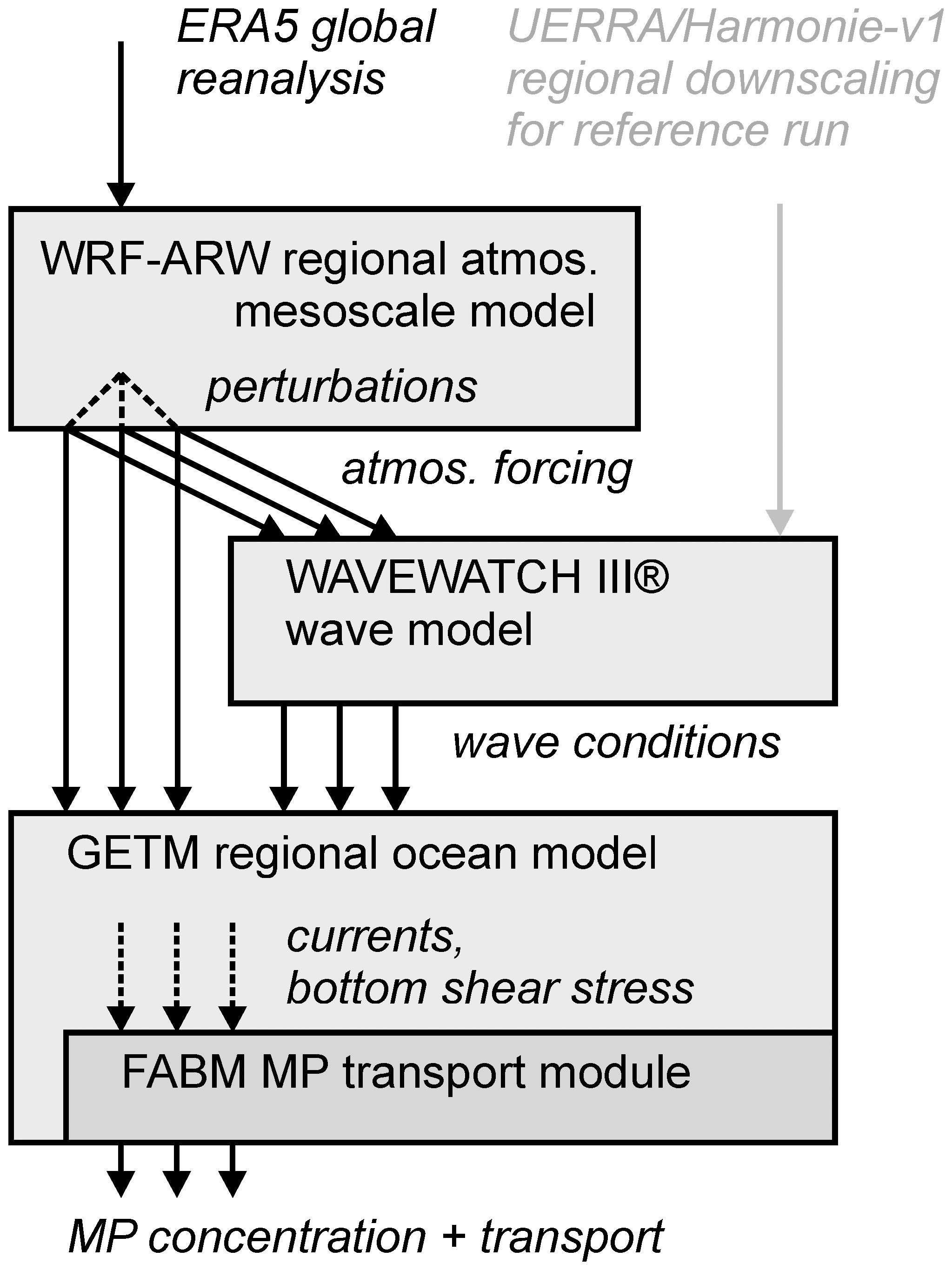
For our assessment, we applied a four-step model chain, as illustrated in Fig. 1. Firstly, ensemble data based on stochastic perturbations were produced with the WRF-ARW (Weather Research and Forecasting Model in the Advanced Research WRF variant) atmospheric model to account for uncertainties in the representation of storm events. Secondly, the atmospheric fields were passed to the WAVEWATCH III^® wind wave model. Thirdly, atmospheric and wave ensemble data were then applied to drive the GETM (General Estuarine Transport Model) regional ocean model. Finally, a transport module in GETM simulated the transport of PET and PVC with particle sizes of 10 and 330 µm. The WRF-ARW atmospheric model was applied here to produce an ensemble hindcast of a storm surge event in the Baltic Sea and to provide the necessary forcing fields for the wave and the ocean model. The simulation period covered 1–4 January 2019. This includes the storm Alfrida (the reader is referred to the ECMWF Severe Event Catalogue: https://confluence.ecmwf.int/pages/viewpage.action?pageId=129123779, last access: 2 April 2020) which moved across southern Sweden and especially hit the island of Gotland, where wind speeds of 27.5 m s⁻¹ (10 Bft) were reached (The Local, 2019). Storms of this strength occur approximately two to three times per year in the Baltic Sea, although at different locations. WAVEWATCH III^® was used to produce ensemble hindcasts of wave parameters based on the WRF-ARW output. GETM was driven by the ensemble hindcasts of the corresponding atmospheric and wave parameters from the unperturbed and perturbed model runs.

Figure 1 Schematic overview of the model chain used in this study.

2.1 The WRF-ARW atmospheric model

Version 4.1.1 of the WRF-ARW atmospheric mesoscale model (https://github.com/wrf-model/WRF/releases, last access: 14 March 2020) (Skamarock et al., 2019) was used in this study for ensemble hindcasting. A region slightly larger than the Baltic Sea was used with a horizontal resolution of about 0.063^∘, and output was written every 5 min. Vertically, 89 pressure levels were applied up to 50 hPa, corresponding to levels 2 to 90 in the ERA5 reanalysis (Copernicus Climate Change Service(C3S), 2017). Initial and lateral boundary conditions originated from the ERA5 reanalysis. Osinski and Radtke (2020) tested different ensemble generation strategies with WRF-ARW driven by ERA5 and compared the outcome with the uncertainty measure provided by the ERA5 reanalysis. As demonstrated in Osinski and Radtke (2020), stochastic perturbations, namely stochastically perturbed parameterization tendencies (SPPT; Buizza et al., 1999) and stochastic kinetic energy backscatter (SKEB; Shutts, 2005), were used here to produce a small ensemble of 30 members to study the impact of the uncertainty in the atmospheric forcing on the transport patterns, which includes random perturbations of the lateral boundary conditions (Skamarock et al., 2019). Instead of validating the atmospheric data against observations, the wind data were validated indirectly by the wave model output. A visual comparison of the WRF-ARW wind fields against UERRA/HARMONIE-v1 and ERA5 data can be found in Osinski and Radtke (2020).

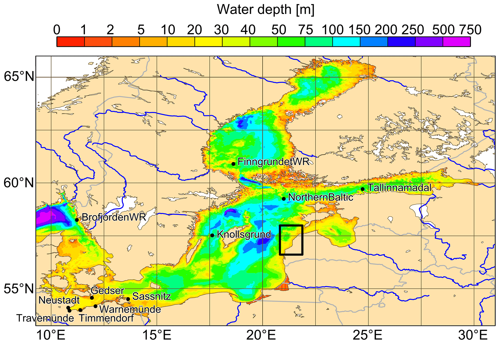
Figure 2 Bathymetry [m] of the 1 nautical mile WAVEWATCH III^® set-up. Black dots show stations for the validation of water level and significant wave height. The black rectangle shows the subregion for plots of the transport simulation results.

Sources of uncertainty in atmospheric model predictions originate from the initial conditions and from the model physics; for a regional model, they also originate from lateral boundary conditions. Osinski and Radtke (2020) compared different ensemble generation methods and proposed the use of the ERA5 data from the Ensemble of Data Assimilations as initial conditions to allow for a spread from the start of the simulation. The initial conditions in the presented study are based on the high-resolution ERA5 reanalysis, and the model approach includes perturbations of the model physics and the lateral boundary conditions. In contrast, the desired spread needs to develop in the model ensemble in the method chosen here. We selected this method to keep our results comparable with a potential future application in forecast mode. While we ran the model for a storm event in the past, the same could be done for a predicted storm, possibly based on a deterministic forecast product.

2.2 The WAVEWATCH III^® wind wave model

Wave-induced bottom shear stress is an important driver for the resuspension of bottom sediments and, potentially, of high-density MPs on the seafloor, as investigated in this study. To be able to prescribe wave parameters at high spatial and temporal resolution, the WAVEWATCH III v6.07^® (https://github.com/NOAA-EMC/WW3 third-generation spectral wind wave model, last access: 14 March 2020) (Tolman, 1991; The WAVEWATCH III® Development Group (WW3DG), 2019) was applied in a three-level one-way nested configuration. The model domain with the highest resolution is based on the same grid as in the GETM model (Gräwe et al., 2019). Dissipation and wind input were based on the formulation of Ardhuin et al. (2010), and the SHOWEX bottom friction scheme was applied following Ardhuin et al. (2003). For the latter, a map of the D50 (median diameter of the particle size distribution) sediment grain size was prescribed based on the European Marine Observation and Data Network (EMODnet; http://www.emodnet-geology.eu/, last access: 14 March 2020) data. The wave spectrum was discretized in the same way as in the ERA5 reanalysis: 24 directions starting at 7.5^∘ with a 15^∘ direction increment, and 30 frequencies starting at 0.03453 Hz geometrically distributed with a step of 1.1. A set-up with a 0.1^∘ resolution covering the North Sea and a small part of the eastern Atlantic Ocean was used to produce boundary conditions for the Baltic Sea set-up at the border with the North Sea. The 0.1^∘ model was nested into a set-up for the Atlantic Ocean with a 0.5^∘ resolution. The GEBCO_2014 Grid, version 20150318 (http://www.gebco.net, last access: 14 March 2020), was used as bathymetry for the Atlantic and North Sea set-ups. The Baltic Sea set-up had a resolution of 1 nautical mile with a bathymetry based on the work of Seifert et al. (2001). The 0.5^∘ set-up is driven by ERA5 winds and the ERA5 sea ice cover fraction. For the 0.1^∘ set-up, UERRA/HARMONIE-v1 (Ridal et al., 2017) winds and the ERA5 sea ice cover fraction were used because of their higher spatial resolution. The Baltic Sea set-up was driven by two data sets: the UERRA/HARMONIE-v1 wind for a reference simulation, and the wind produced with the WRF-ARW wind ensemble for the MP ensemble simulations. Sea ice was taken from the Ostia reanalysis (http://marine.copernicus.eu/services-portfolio/, last access: 29 November 2020). An obstruction grid based on the GSHHS (Global Self-consistent, Hierarchical, High-resolution Shorelines) (Wessel and Smith, 1996) coastline data set has been generated with the Gridgen software (https://github.com/NOAA-EMC/gridgen, last access: 14 March 2020) to take unresolved orography into account.

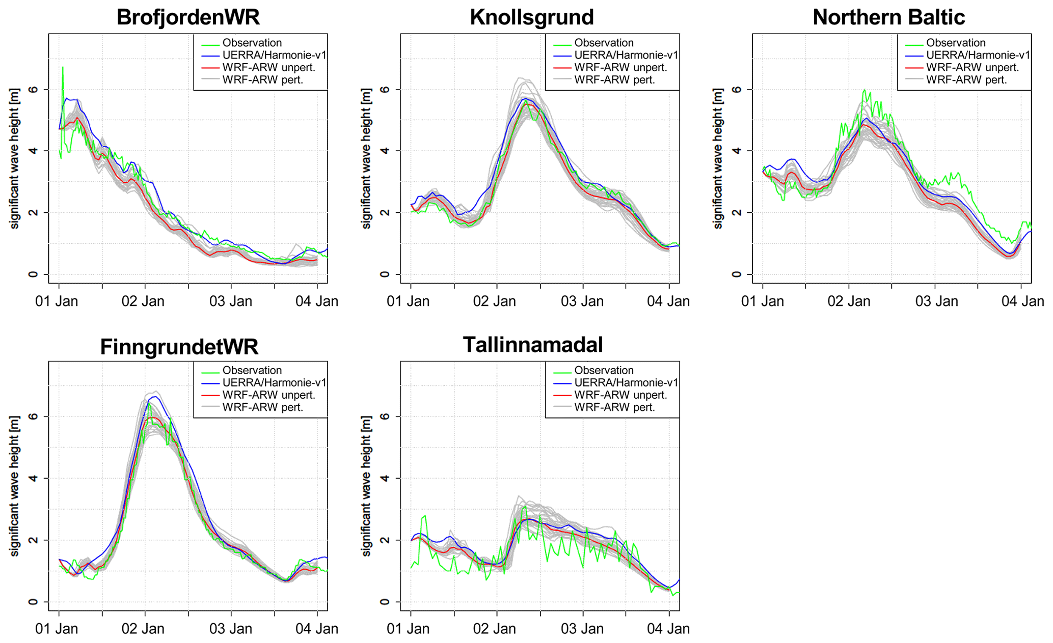
Figure 3 Significant wave height at five stations from the 1 nautical mile WAVEWATCH III^® model run. Wind data are from UERRA/HARMONIE-v1, WRF-ARW is unperturbed, and the 30 WRF-ARW members are generated with stochastic perturbations.

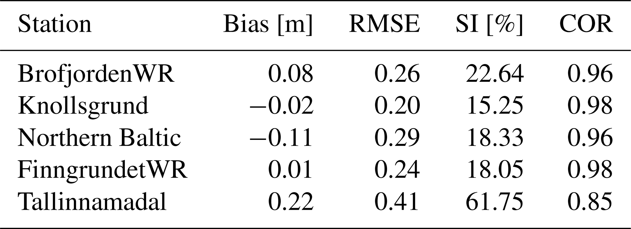
Observation data from buoys available from the Copernicus Marine Environment Monitoring Service (http://marine.copernicus.eu/services-portfolio/access-to-products/, last access: 14 March 2020) (CMEMS) were used for validation and calibration. A comparison with station data in Fig. 3 shows good agreement in the significant wave height as well as verification scores over January 2019 (Table 1). The spread in the ensemble is visible at all stations and is expected to provoke differences in the bottom shear stress, leading to differences in the resuspension.

Table 1 Verification scores – root mean square error (RMSE), scatter index (SI, Zambresky, 1989), and correlation (COR) – for significant wave height simulated by WAVEWATCH III^® driven by UERRA/HARMONIE-v1 for January 2019.

Waves affect the seafloor until a water depth of about half the wave length. The dominant wavelength in the Baltic Sea is between 20 and 70 m and can reach up to 130 m (Kriaučiūnienė et al., 1961).

2.3 The GETM regional ocean model

GETM (General Estuarine Transport Model; Burchard and Bolding, 2002; Hofmeister et al., 2010; Klingbeil and Burchard, 2013) is an ocean model specifically designed for the coastal ocean (see review by Klingbeil et al., 2018). In the present study, GETM was applied to the Baltic Sea with the model set-up of Gräwe et al. (2019), on the same 1 nautical mile grid as the innermost WAVEWATCH III^® nest. The model domain is shown in Fig. 2. The original set-up was extended by coupling it to FABM (Framework for Aquatic Biogeochemical Models; Bruggeman and Bolding, 2014) in order to consider sediment and MP. For an accurate 3-D transport of these quantities, GETM provides high-order advection schemes with reduced spurious mixing (Klingbeil et al., 2014), a state-of-the-art second-moment turbulence closure for vertical mixing from GOTM (General Ocean Turbulence Model; Burchard et al., 1999; Umlauf and Burchard, 2005), and flow-dependent lateral mixing (Smagorinsky, 1963). Numerical mixing leads to an unrealistically high diffusion of transported concentrations, reducing the peak concentrations and overestimating the area in which tracers spread. The accuracy of the model is further increased by adaptive vertical coordinates that guarantee an optimal vertical mesh aligned to the dynamic boundary layers and to the stratified interior (Gräwe et al., 2015). Air–sea fluxes were calculated from the meteorological data provided by the atmospheric model according to the bulk formulas of Kondo (1975). Based on the data provided by the wave model, GETM calculated the mean and maximum combined wave- and current-induced bed stress during a wave cycle. The latter was used in FABM for the erosion of sediment and MPs from the bottom pool (see Sect. 2.4). A realistic initial state as the starting condition for the hydrodynamical model was obtained by prolonging the simulations from Gräwe et al. (2019) with the UERRA/HARMONIE-v1 atmospheric data set. Further details about open boundary conditions and river discharge can be found in Gräwe et al. (2019).

A detailed validation of the model set-up can be found in Gräwe et al. (2019) and (). For demonstration purposes, only the spread in sea surface elevation due to the different atmospheric forcing sets is shown here (Fig. 4). A verification of the water level at different stations from EMODnet (https://www.emodnet-physics.eu/, last access: 14 March 2020) showed satisfactory performance for both forcing data sets (WRF-ARW and UERRA/HARMONIE-v1). A large spread is also visible in the water level, especially at the peak of the surge.

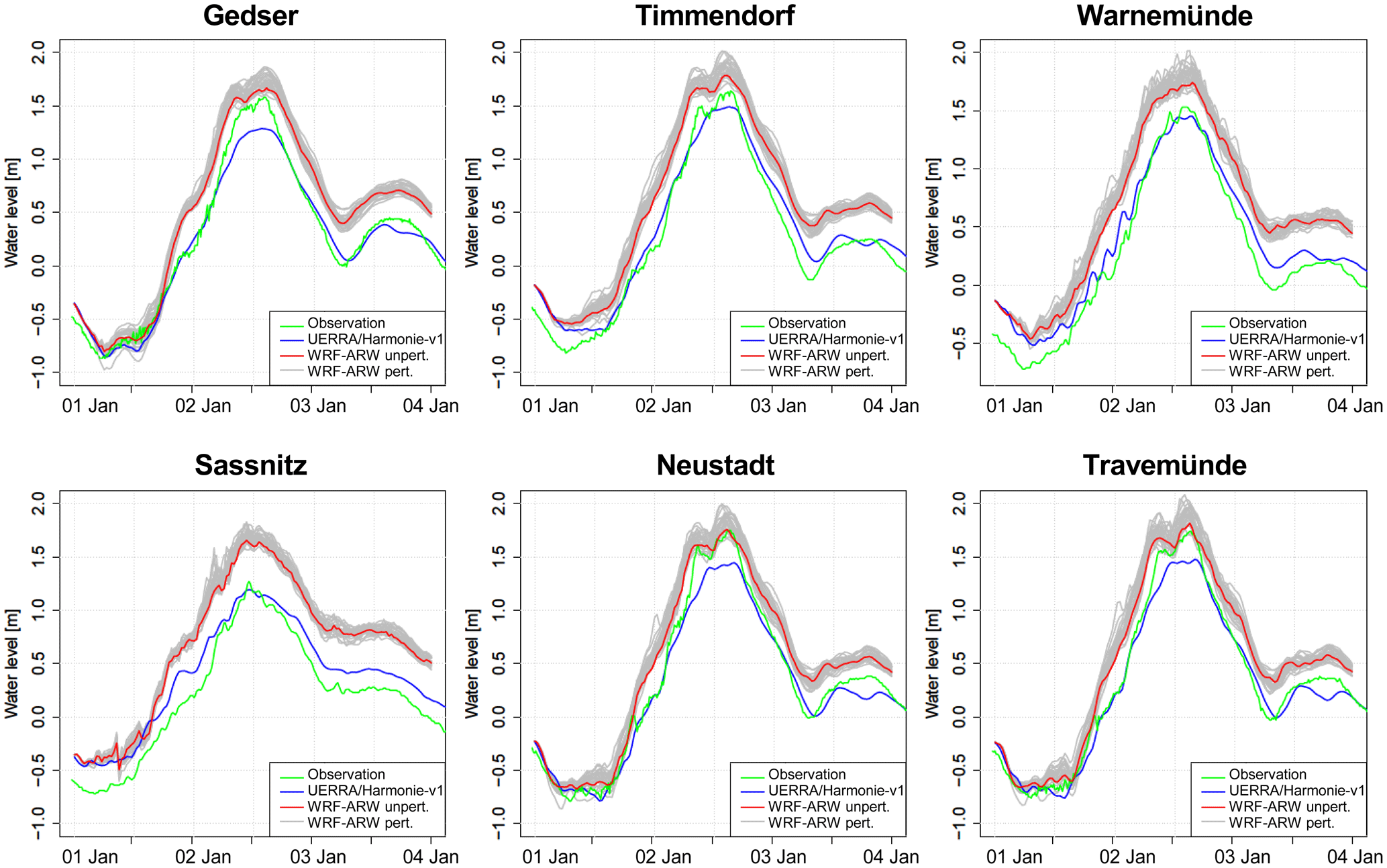
Figure 4 Water level at six stations with the 1 nautical mile GETM model; atmospheric data from UERRA/HARMONIE-v1, WRF-ARW is unperturbed, and the 30 WRF-ARW members are generated with stochastic perturbations.

The ensemble generation in the GETM model in this study is only based on the ensemble hindcasts of the atmospheric and wave parameters driving the model runs. Brankart et al. (2015) showed that stochastic perturbations in the ocean model are also important for uncertainty estimation. The uncertainty in the ocean currents could therefore be underestimated.

2.4 Microplastic representation

In GETM and FABM, sediment and MPs are represented as Eulerian concentration fields. GETM simulated the 3-D transport of the pelagic concentrations, whereas the FABM model calculated the interaction with the corresponding bottom pools due to erosion and deposition and provided settling velocities to GETM. In FABM, a model for non-cohesive sediments (see  Sassi et al., 2015) was used to calculate erosion, settling, and deposition of both sediment and MPs. The different transport was caused by the lower densities of MPs, which exceed that of the ambient water, i.e. we only considered sinking particles. This study focuses on model MPs with the sizes and densities reported by Stuparu et al. (2015): 10 and 330 µm for both PVC with a density of 1275 kg m⁻³ and PET with a density of 1400 kg m⁻³. To study the impact of density and particle size on the uncertainty in the transport, additional densities of 1100, 1200, and 1300 kg m⁻³ and particle sizes of 200, 250, 300, and 350 µm were tested. As our main aim is to support measurement campaigns and larger particles are easier to sample, we focus our attention on particles above 300 µm.

The simulations in this study started from homogenous bottom pools of 1 kg m⁻² as a purely hypothetical reference value as well as zero suspended material in the water column. Rivers and open boundaries were assumed to not import material into the model domain. MP transport in the model is affected by wave activity and different types of currents. Tidal currents are represented, but they only play a role in the Danish straits, as the interior of the Baltic Sea is non-tidal. Turbidity currents cannot be represented in our model, as the concentration of suspended matter has no influence on seawater density in the model. Thermohaline circulation, in contrast, is fully taken into account.

3 Results and discussion

3.1 MP relocation and its uncertainty

After a 2 d storm surge event, a rearrangement of particles could be observed in the model with some locations dominated by erosion and others by deposition. This can be seen by the change in the amount of MP stored in the bottom pool (PET and PVC with a diameter of 330 µm). To demonstrate the range of uncertainty in the transported amount of MP, two different grid cells in the Gotland Basin were selected (Fig. 5): 57.69^∘ N, 21.35^∘ E (Fig. 6a–b) as a net erosion location, and 57.66^∘ N, 21.32^∘ E (Fig. 6c–d) as a net deposition location. Relative to the initial concentration, net erosion varied between 39 % and 72 % for PVC and between 16 % and 45 % for PET. Net accumulation varied between −13 % and 38 % for PVC and between 22 % and 34 % for PET. Thus, for PVC in the deposition grid cell (Fig. 6c), weak erosion is visible in some ensemble members, whereas the majority of the ensemble members show net deposition at this location. For the denser PET, the uncertainty range is smaller than for PVC, implying that its transport is less sensitive to uncertainties in the wind fields and more predictable. Still, the transported amount, even in this particle class, varies by around a factor of 2 between realizations, showing that a realistic quantitative estimation of MP transport is impossible in ocean circulation models, even if the precise sinking, settling, and resuspension properties of the MP particles were perfectly known.

3.2 Erosion and deposition areas

Now we consider the spatial patterns where erosion and sedimentation take place. The spatial pattern in four selected ensemble members and the deterministic runs is shown in Fig. 7. We chose four members with a considerable spread in the simulated wave height (Fig. 7g). The overall spatial pattern is very similar between the different realizations. The main impact of the metocean uncertainty lies in the amount of the transported material. The perturbations of the atmospheric model also produce deviations in the track of the storm between ensemble members, which impacts the direction of ocean waves and currents and, in turn, the direction in which the bottom shear stresses are directed. These findings indicate that the bathymetry has a predominant impact on the region where erosion and deposition take place, as the locations are insensitive to changes in the track of the storm. For this specific storm surge event and selected region, net deposition took place on the south-western sides of ridges, and net erosion took place on the north-eastern sides. Model MP with a diameter of 330 µm in deeper regions, below 50 m, was completely unaffected. It is well known that water depth plays a major role in sediment erosion by waves, as deep-water waves (with wavelengths much shorter than the water depth) show an exponential attenuation in their velocity amplitude with depth (e.g. Kundu and Cohen, 2001). Our findings suggest that this causes stability in the spatial patterns of MP transport against changes in the wind forcing and makes the areas where erosion and deposition take place during a specific storm event predictable.

Figure 5 Bathymetry [m] of the subregion for which the model results are presented. Black dots indicate the locations of two selected grid cells for later reference.

Figure 6 Changing bottom concentration of PVC (a, c) and PET (b, d) particles with a 330 µm diameter in the two grid cells indicated in Fig. 5, relative to the initial concentration. The different curves show 30 perturbed runs and 1 unperturbed run with WRF atmospheric forcing and another simulation with UERRA/HARMONIE-v1 forcing. Panels (a) and (b) show a grid cell predominated by processes of net erosion, whereas panels (c) and (d) show a cell with net sedimentation.

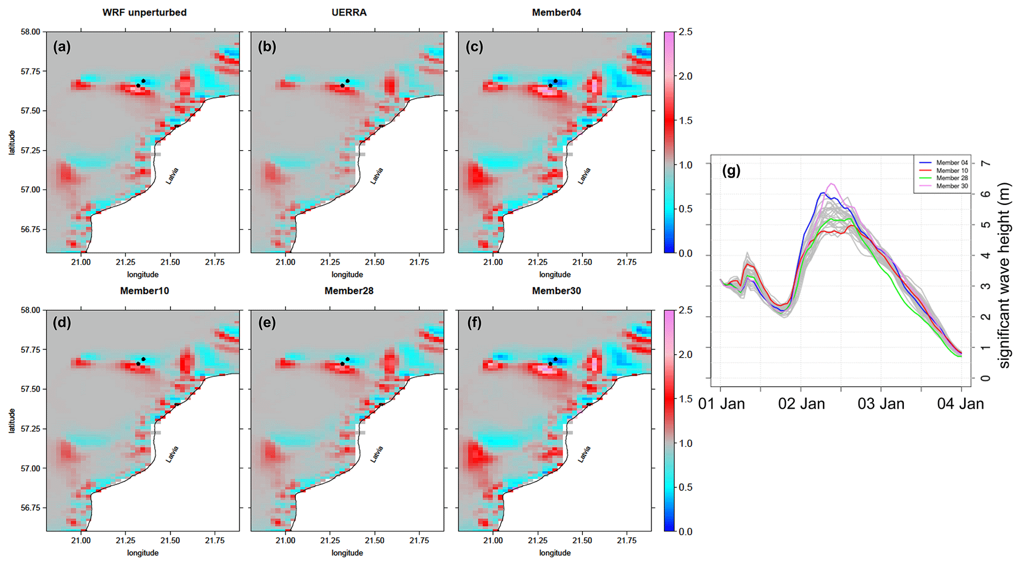
Figure 7 Seabed concentration of PVC with a 330 µm diameter on 3 January 2019 at 12:00 UTC, i.e. after the storm surge event in the model, relative to the homogenous initial concentration. Individual panels show the unperturbed WRF run (a), the model driven by UERRA/HARMONIE-v1 (b), and four selected WRF ensemble members (c–f). Dots show the locations of the grid cells selected in Fig. 6. (g) Time series of the significant wave height [m] at the position of the dot in the other figures with net erosion.

The uncertainty ranges of the spatial pattern of the model results were further investigated by means of the ensemble statistics composed of the mean, minimum, and maximum of each individual grid cell of all ensemble members (Fig. 8). The net effect – whether the location was characterized by deposition or erosion – appeared largely consistent for the entire uncertainty range. Only a few locations showed deviations from this finding where some ensemble members shifted between weak erosional and depositional net effects. The larger extent of the erosional areas was due to more severe representations of the storm event in some ensemble members. Overall, these findings suggest stability in spatial patterns of MP transport against changes in the wind forcing. Areas of erosion and deposition during a specific storm event are predictable.

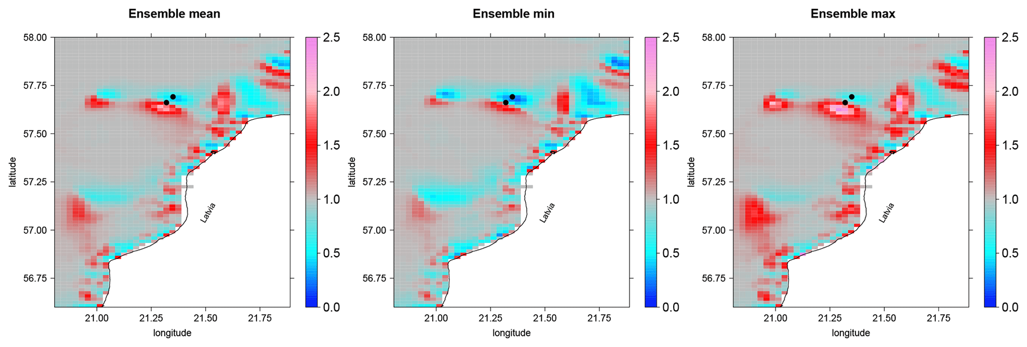
Figure 8 Ensemble mean, minimum, and maximum of the seabed concentration of PVC with a 330 µm diameter on 3 January 2019 at 12:00 UTC, i.e. after the storm surge event in the model, relative to the homogenous initial concentration. Dots show the locations of the grid cells selected in Fig. 6.

3.3 Effect of particle size on transport uncertainty

Next, we investigate the effect of particle size on the uncertainty in the transport by reducing the size of the particles to 10 µm. The small PET particles show a net erosion across almost the whole model domain due to slower resettlement. That is, they are still found in the water column up to 1.5 d after the storm (at the end of the simulation). This partly explains the large difference between the ensemble minimum and maximum (Fig. 9b, c): When sedimentation takes longer, quantitative differences in erosion strength will result in larger transport deviations, as the material can be advected further. This finding is also supported by theory on sediment transport: smaller particles (if unconsolidated) are suspended under lower shear stress levels and also require calmer metocean conditions to deposit. Thus, the uncertainty in MP transport appears to strongly depend on the particle diameter and density.

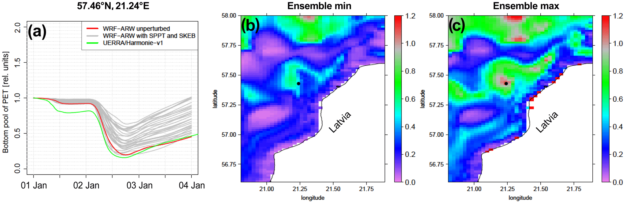
Figure 9 (a) Change in the seafloor concentration of PET particles with a 10 µm diameter in one selected grid cell in 30 perturbed runs and 1 unperturbed run with WRF forcing and 1 run with UERRA/HARMONIE-v1 forcing. (b) Ensemble minimum and (c) ensemble maximum on 4 January 2019 at 00:00 UTC (at the end of the simulation). All concentrations are relative to the homogenous initial concentration. The black dots show the locations for the time series plots.

To find out whether this is a systematic effect, the uncertainties in the amount of transported material dependent on the particle properties size and density were investigated in more detail. These relationships were studied based on sensitivity runs with 30 ensemble members for (1) PVC with grain sizes of 200, 250, 300, and 350 µm as well as (2) 330 µm MP with different densities of 1100, 1200, 1300, and 1400 kg m⁻³ (Fig. 10a, b). The seafloor concentrations at the end of the model run deviate between the ensemble members. Relative deviations from the ensemble mean were calculated. Figure 10c and d show that the relative uncertainty increases with decreasing density and/or particle diameter, with the exception of the 1100 µm MP class, which shows a smaller uncertainty as it is almost completely resuspended at the chosen location. We conclude that the uncertainty in the amount of transported material on the seafloor at a specific time depends strongly on the properties of the transported material. Thus, the application of an ensemble approach (using more than one model realization to predict transport pathways) is especially important if finer and lighter material is to be represented in future model applications.

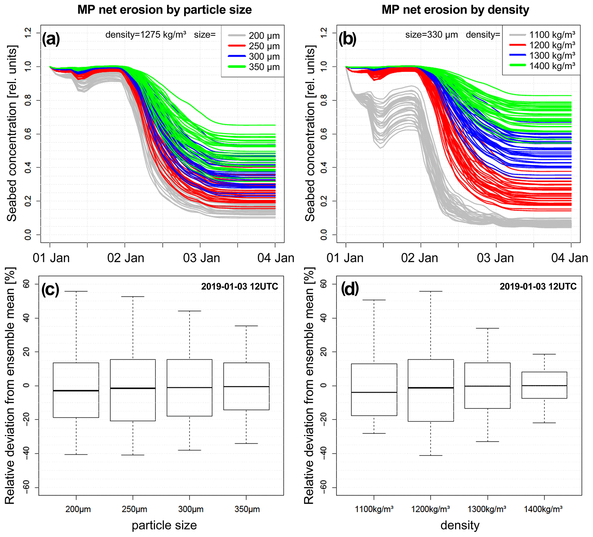
Figure 10 Time series of 30 ensemble members at 57.69^∘ N, 21.35^∘ E for (a) different MP sizes and (b) different MP densities. (c, d) Box-and-whisker plots show the uncertainty in the concentration of material on the seabed, expressed as a relative deviation of the individual ensemble members from the ensemble mean.

Figure 11 Spread of runs with varying atmospheric forcing and/or varying wave forcing for PVC with a 330 µm diameter (a, b, c) and PET with a 10 µm diameter (d, e, f), for the bottom concentration at 57.69^∘ N, 21.35^∘ E (see Fig. 9) relative to the initial value.

3.4 Pathways of atmospheric uncertainty propagation

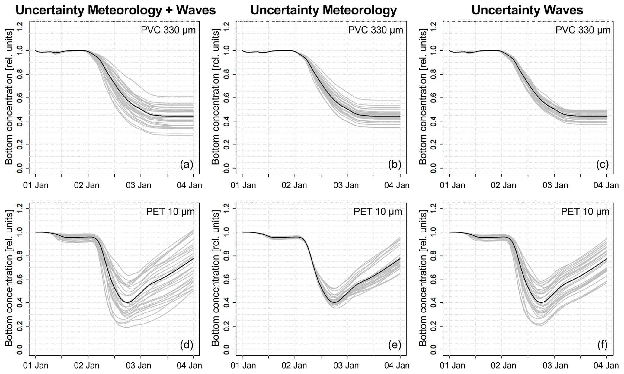
In the following, the mechanism by which the atmospheric uncertainty affects the MP transport is identified. In our model, this can be caused (a) by influencing the wave height, which changes the bottom shear stress and, therefore, MP mobilization, or (b) by directly affecting the ocean circulation through factors such as momentum input, thereby influencing both mobilization and transport. We focused on these two major pathways and attempted to distinguish their influence. The possibility of interlinkage by wave–current interaction is neglected in the present model cascade. To estimate the respective uncertainties of MP transport of the two above-mentioned pathways, an ensemble driven with the wave data from the unperturbed WRF-ARW run with the perturbed WRF-ARW atmospheric forcing and vice versa (with perturbed wave data and unperturbed atmospheric data) has been conducted. By comparing (Fig. 11) the outcome with the original ensemble, where both perturbed atmospheric and wave data were used, it can be seen that the impact of the wave field depends on the properties of the transported material. The lighter or smaller the MP, the more important the impact of the wave uncertainty on the amount of transported material. For denser and larger MP, the uncertainty in the direct effect of atmospheric uncertainty on hydrodynamics is predominant.

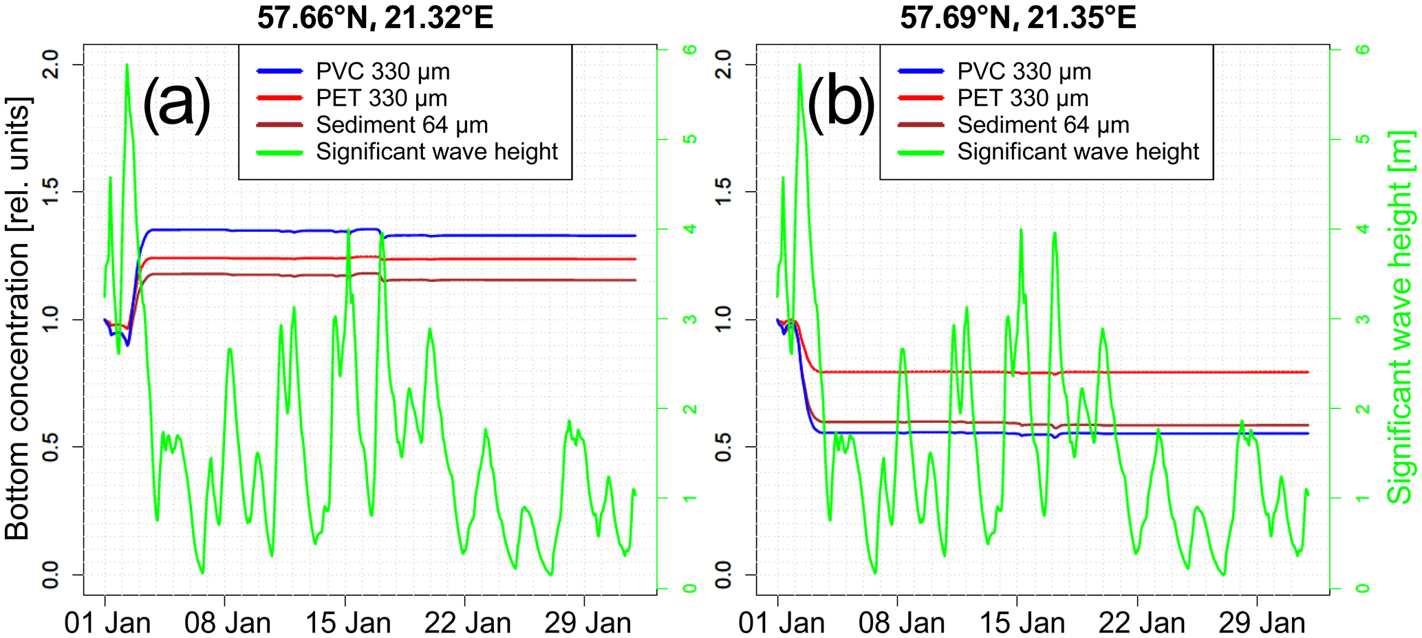
Figure 12 Evolution of the amount of PET and PVC with a 330 µm diameter and sediment with a 64 µm diameter on the seafloor during January 2019, starting from initial amount of 1 kg m⁻², at two grid cells, (a) with net deposition and (b) with net erosion.

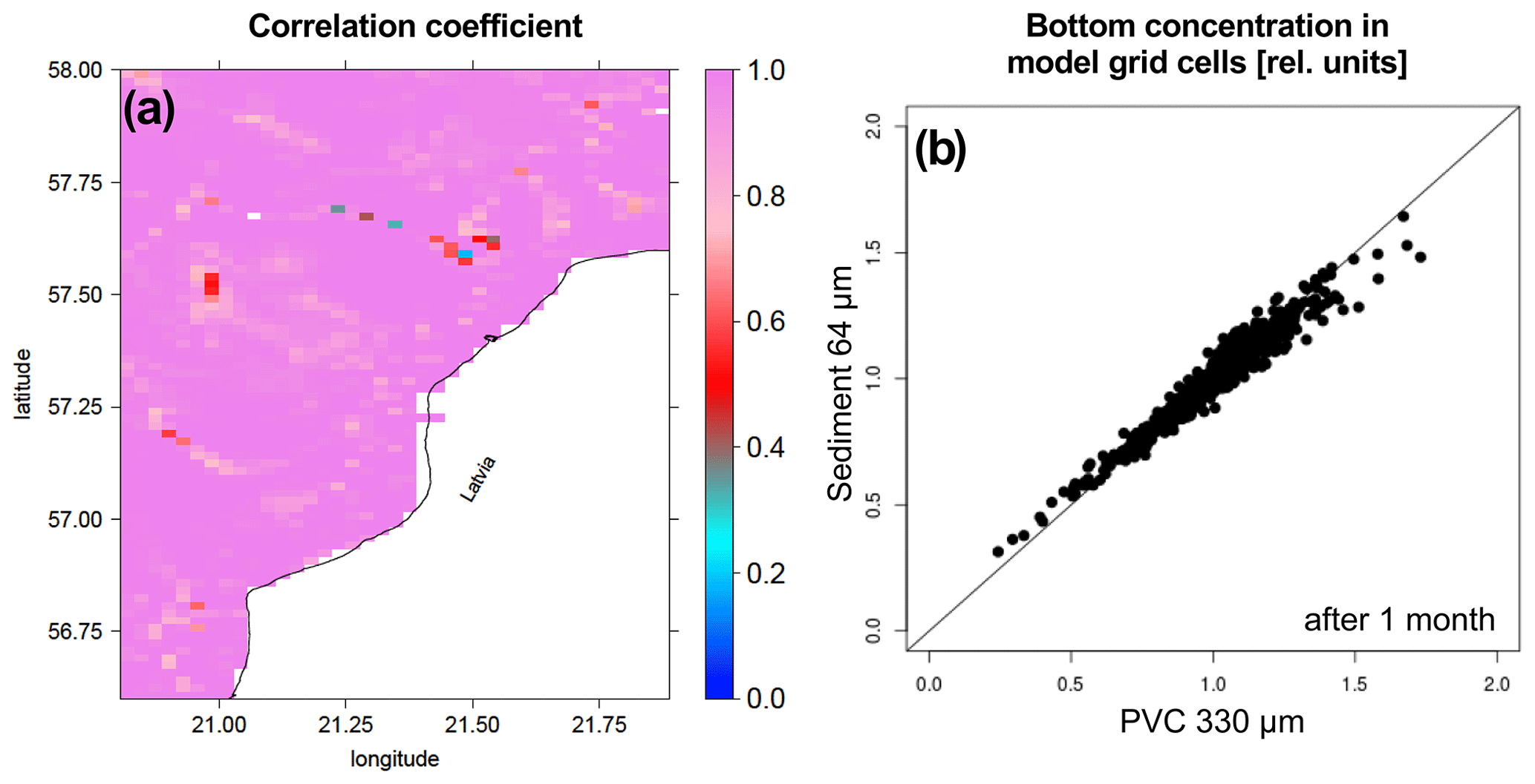
Figure 13 (a) Pearson correlation between the time series of bottom concentrations of PVC with a 330 µm diameter and sediment with a 64 µm diameter for January 2019. (b) Scatter plot of bottom concentrations after the 1-month simulation. Concentrations are given relative to the homogenous initial concentration.

3.5 Importance of storms for MP transport

Higher-density MPs of about 300 µm diameter were only transported under severe storm conditions, as demonstrated in Fig. 12. The continuation of the simulation for the rest of January 2019 caused almost no further erosion or deposition. This confirms the assumption regarding the importance of extreme events for MP transport, which complicates its direct empirical determination. Budget methods will be required to empirically determine quantities of transported MP. A budget method relates (a) the input and (b) the output of a quantity to (c) changes in its mass, e.g. inside an area of interest. If two of the three values are known, the third one can be determined. That is, transport rates might be more reliably derived from observed amounts before and after storm events than by multiplying abundances of suspended MP by instantaneous volume transports, both of which might show strong temporal variation during extreme weather conditions.

3.6 Similarities between MP and sediment transport

The finding that spatial patterns of MP can be reliably predicted by ocean models, while the quantitative estimation of MP is prone to considerable uncertainties shows that additional approaches are required for a more reliable estimation of large-scale MP concentration levels. Here, the recently found MP–sediment proxy postulated by Enders et al. (2019), which is based on correlations between certain high-density polymer size fractions (> 1000 kg m⁻³, > 500 µm) and sediment grain size fractions, would be an achievable method. Estimations of MP levels can be based on a relatively small in situ data set and extrapolated to larger spatial scales by using the MP–sediment correlates. Lower densities of MP (1000–1600 kg m⁻³) compared with sediments (quartz: 2650 kg m⁻³) are offset by a larger size. This relationship was explained by comparable threshold bed shear stresses (and thus erosion rates) between these size fractions, which appeared to be the predominant mechanism determining the sorting in the described study area (Warnow Estuary, Baltic Sea, Germany; Enders et al., 2019). Although the MP size ranges covered in the present study were below those investigated by Enders et al. (2019), it is assumed that similar patterns can be found for smaller size ranges. Indeed, in the present study, after the storm surge event, model PVC with a diameter of 330 µm co-occurred with 64 µm sediment grains, as apparent by the high correlation coefficient shown in Fig. 13. This correlation is found to be largely explained by similar erosion rates (Fig. 12b), whereas bottom concentrations, predominantly determined by deposition, are also influenced by the settling velocity of particles and, thus, differ slightly (higher amounts of PVC). Therefore, it is expected that areas largely influenced by the settling of MP show a larger difference in the expected MP–sediment size relation than described by the current MP–sediment proxy. For instance, larger (and/or heavier) MP particles than 330 µm PVC (such as PET) would be closer to the deposition rate of sediment grains of 64 µm (Fig. 12a). Existing maps of sediment substrate type, which typically differentiate between median grain sizes above and below 63 µm (e.g. EMODnet, 2020), may therefore also provide information about the MP concentrations to be expected. However, as this investigation is purely based on our model results with the above-mentioned uncertainties, in situ measurements are inevitable to further research the influences on this MP–sediment proxy.

4 Conclusions

A storm surge event in the Baltic Sea in January 2019 has been hindcast by a four-step probabilistic model chain started from an homogeneous initial MP distribution. The model validation showed a good performance for water level and significant wave height compared with different station data.

A strong variation in the amount of transported MP between ensemble members was found. This illustrates that quantitative modelling of MP transport during storm events already exhibits substantial uncertainty due to uncertainties in meteorological forcing fields (e.g. wind speeds). A test with different particle sizes and densities showed a dependence of the uncertainty in the transport on the particle properties. The impact of the metocean uncertainty on sediment and MP transport increases with decreasing particle density and/or size.

The spatial distribution pattern where material was eroded or accumulated in the model runs was stable against the atmospheric perturbations, illustrating the capability of a numerical model to identify regions of interest where seafloor sampling of MP concentrations is promising.

The demonstrated procedure could also be applied in forecast mode, by exchanging the ERA5 reanalysis data used in this study for data such as the freely available GFS forecasts (https://www.emc.ncep.noaa.gov/emc/pages/numerical_forecast_systems/gfs.php, last access: 14 March 2020). As a synoptic-scale winter storm event can be well predicted at medium-range timescales (3–5 d), this would allow for the production of ensemble simulations of MP transport a couple of days in advance in order to identify sampling regions, as a strategic support tool for measurement campaigns. The impact of the uncertainty from the lack of knowledge on settling velocities and critical bottom shear stresses would then have to be taken into account. One idea to reduce the necessary computational resources is a clustering of the atmospheric ensemble data and driving the rest of the model chain (wave and ocean model) with a reduced set of representative ensemble members.

As a consequence of the insensitivity of the location of erosional and depositional areas to the uncertainty in the metocean forcing and a substantially smaller transport during moderate conditions, this study indicates that it would, in principle, be possible to construct a map of the spatial distribution of high-density MP particles in the Baltic Sea using long model runs containing several storm events. Differences between storm events might be larger than the uncertainty in a single event. To get a more general picture of erosional and depositional regions in the Baltic Sea, other storm events with different tracks also have to be taken into account.

The demonstrated ensemble approach can also be useful for other applications, such as implementation in the maritime transport sector. After a strong storm event, it could help to predict whether it would still be possible for large vessels to enter a harbour or whether the morphodynamic changes are so strong that dredging would be necessary.

Appendix A: Mathematical description of the particle sinking and erosion model

Sinking velocity of the particles is initially calculated using the Stokes formula:

$$\begin{array}{}\text{(A1)}& w_{\mathrm{Stokes}}={\displaystyle \frac{g{D}^{\mathrm{2}}}{\mathrm{18}\mathit{\nu }}}{\displaystyle \frac{{\mathit{\rho }}_{\mathrm{p}}-{\mathit{\rho }}_{\mathrm{w}}}{{\mathit{\rho }}_{\mathrm{w}}}},\end{array}$$

where g is the gravitational acceleration, D is the particle diameter, ν is the kinematic viscosity of water, and ρ_p and ρ_w are the densities of the particle and the water respectively. To correct for larger particles whose sinking velocity would be overestimated by the Stokes formula, a Newtonian correction is applied by an iterative algorithm:

• a Reynolds number is calculated as $\mathit{\text{Re}}=\mathrm{0.64}{w}_{\mathrm{sink}}D/\mathit{\nu }$;

• a relative drag coefficient is derived from this Reynolds number as $C_{\mathrm{D}}=\mathrm{18.5}/{\mathit{\text{Re}}}^{\mathrm{0.6}}$ following Perry and Chilton, as cited by Khalaf (2009);

• the updated velocity is calculated as $w_{\mathrm{sink}}=\sqrt{\frac{\mathrm{4}gD}{\mathrm{3}{C}_{\mathrm{D}}}\frac{{\mathit{\rho }}_{\mathrm{p}}-{\mathit{\rho }}_{\mathrm{w}}}{{\mathit{\rho }}_{\mathrm{w}}}}$, which can be understood as a weighted geometric mean between the two velocities w_Stokes and ν∕D.

This correction makes large particles sink slower than the Stokes formula suggests. However, we also erroneously applied the correction to the small particles where it resulted in an undesired upward correction. This has no effect on particle erosion, but it accelerates redeposition, which may even lead to an underestimation of the influence of meteorological uncertainty for the small particles in our study.

Erosion takes place when the actual shear stress exceeds the critical shear stress. To determine the critical shear stress, we follow the Shields curve, using the version that was corrected by Soulsby (1997). First, we calculate the dimensionless particle diameter D_*, which relates the particle diameter D to a viscosity-determined length scale, following Rijn (1984):

$$\begin{array}{}\text{(A2)}& D_{*}=\sqrt{\mathrm{3}}{\displaystyle \frac{g}{{\mathit{\nu }}^{\mathrm{2}}}}{\displaystyle \frac{{\mathit{\rho }}_{\mathrm{p}}-{\mathit{\rho }}_{\mathrm{w}}}{{\mathit{\rho }}_{\mathrm{w}}}}D,\end{array}$$

where ν is the kinematic viscosity of water, ρ_p is the particle density, and ρ_w is the water density. Then, we calculate the critical Shields parameter for non-cohesive grains, θ_cr (also dimensionless), following Soulsby (1997) as cited by Ziervogel and Bohling (2003):

$$\begin{array}{}\text{(A3)}& {\mathit{\theta }}_{\mathrm{cr}}={\displaystyle \frac{\mathrm{0.3}}{\mathrm{1}+\mathrm{1.2}{D}_{*}}}+\mathrm{0.055}\cdot \left(\mathrm{1}-e^{-\mathrm{0.02}{D}_{*}}\right).\end{array}$$

The critical shear stress can then be calculated as

$$\begin{array}{}\text{(A4)}& {\mathit{\tau }}_{\mathrm{cr}}=D\left({\mathit{\rho }}_{\mathrm{p}}-{\mathit{\rho }}_{\mathrm{w}}\right){\mathit{\theta }}_{\mathrm{cr}}.\end{array}$$

The actual shear stress is calculated from the wave-induced and the current-induced shear stress, τ_w and τ_c respectively. The current-induced shear stress itself, however, is also modified by the wave field, as it changes the bottom drag coefficient according to the DATA2 formula given by Soulsby (1997):

$$\begin{array}{}\text{(A5)}& {\mathit{\tau }}_{\mathrm{m}}=\left(\mathrm{1}+\mathrm{1.2}{\left({\displaystyle \frac{{\mathit{\tau }}_{\mathrm{w}}}{{\mathit{\tau }}_{\mathrm{c}}+{\mathit{\tau }}_{\mathrm{w}}}}\right)}^{\mathrm{3.2}}\right){\mathit{\tau }}_{\mathrm{c}},\end{array}$$

where τ_c is the shear stress induced by the current in the absence of waves. The shear stresses induced by currents and waves are combined depending on the angle α between currents and waves:

$$\begin{array}{}\text{(A6)}& {\mathit{\tau }}^{\mathrm{2}}={\mathit{\tau }}_{\mathrm{w}}^{\mathrm{2}}+{\mathit{\tau }}_{\mathrm{m}}^{\mathrm{2}}+\mathrm{2}{\mathit{\tau }}_{\mathrm{w}}{\mathit{\tau }}_{\mathrm{m}}\cos \left(\mathit{\alpha }\right).\end{array}$$

If the actual shear stress exceeds the critical one, the deposited material becomes resuspended with first-order kinetics, i.e. proportional to its mass in the sediment pool.

The actual values for sinking velocities and critical stresses depend on temperature, as it influences sea water viscosity. Values for 10 ^∘C are presented in Table A1.

Table A1 Sinking velocities and critical shear stress in the model at 10 ^∘C.