the Creative Commons Attribution 4.0 License.
the Creative Commons Attribution 4.0 License.
 | 23 Nov 2020
Multidecadal preconditioning of the Maud Rise polynya region
Henk A. Dijkstra
In this paper, we consider Maud Rise polynya formation in a long (250-year) high-resolution (ocean 0.1∘, atmosphere 0.5∘ horizontal model resolution) of the Community Earth System Model. We find a dominant multidecadal timescale in the occurrence of these Maud Rise polynyas. Analysis of the results leads us to the interpretation that a preferred timescale can be induced by the variability of the Weddell Gyre, previously identified as the Southern Ocean Mode. The large-scale pattern of heat content variability associated with the Southern Ocean Mode modifies the stratification in the Maud Rise region and leads to a preferred timescale in convection through preconditioning of the subsurface density and consequently to polynya formation.
- Article
(11105 KB) - Full-text XML
- BibTeX
- EndNote


A polynya is an open-water area enclosed by sea ice which persists at least for a few months. A famous area for polynya formation is the Maud Rise region in the Weddell Sea. Polynyas occurring at this location are usually referred to Maud Rise polynyas (MRPs), referring to the bathymetry feature below the ocean water. In 1974, the first MRP was observed and developed into the larger Weddell polynya in the following years (Carsey, 1980). These polynyas were observed by in situ (Gordon, 1978) and satellite microwave imaging (Carsey, 1980). The mid-1970s polynya was characterised by a sea-ice-enclosed open-water area (1–3 × 10⁵ km2) located near 65∘ S, 0∘ E (Gordon, 1978). The interest towards polynyas has increased recently because of the appearance of an MRP in the austral winter and spring of 2017, with an open-water area of about 0.5 × 10⁵ km2 (Campbell et al., 2019).
Many observational, modelling and theoretical studies based on the 1974–1976 polynya have addressed its formation, evolution and decay (Martinson et al., 1981; Parkinson, 1983; Holland, 2001; Gordon et al., 2007; Martin et al., 2013; Latif et al., 2017; Weijer et al., 2017; Kurtakoti et al., 2018). The occurrence of convection in the vicinity of Maud Rise is clearly a generic aspect during MRP formation. Convective events are induced by a destabilisation of the water column and the classical view is that surface salinity anomalies (e.g. through brine rejection) induce convection once the column is preconditioned through subsurface processes (Martinson et al., 1981). In Gordon et al. (2007), it is proposed that a negative phase of the Southern Annular Mode (SAM) causes drier atmospheric conditions (net evaporation), resulting in a more saline surface layer, leading to a destabilisation of the water column. Preconditioning can also occur due to the interaction of an ocean eddy and the Maud Rise topographic feature (Holland, 2001) and by stratified Taylor columns (Alverson and Owens, 1996; de Steur et al., 2007).
The occurrence of Southern Ocean convection is also ubiquitous in many global climate models (GCMs). Martin et al. (2013) show that in the Kiel Climate Model (KCM), a centennial timescale buildup of a heat reservoir at mid-level depths (1000–3000 m) preconditions the water column affecting convection. Reintges et al. (2017) analysed a variety of (Coupled Model Intercomparison Project phase five; CMIP5) GCMs and found that several models display deep convection events at multidecadal timescales, for example, the Geophysical Fluid Dynamics Laboratory Climate Model (GFDL-CM) (Zanowski et al., 2015; Zhang and Delworth, 2016). Reintges et al. (2017) argue that models with a weak (strong) stable stratification tend to have a shorter (longer) reoccurrence time of deep convection and demonstrate the importance of sea-ice volume on the average length of both non-convective and convective periods.
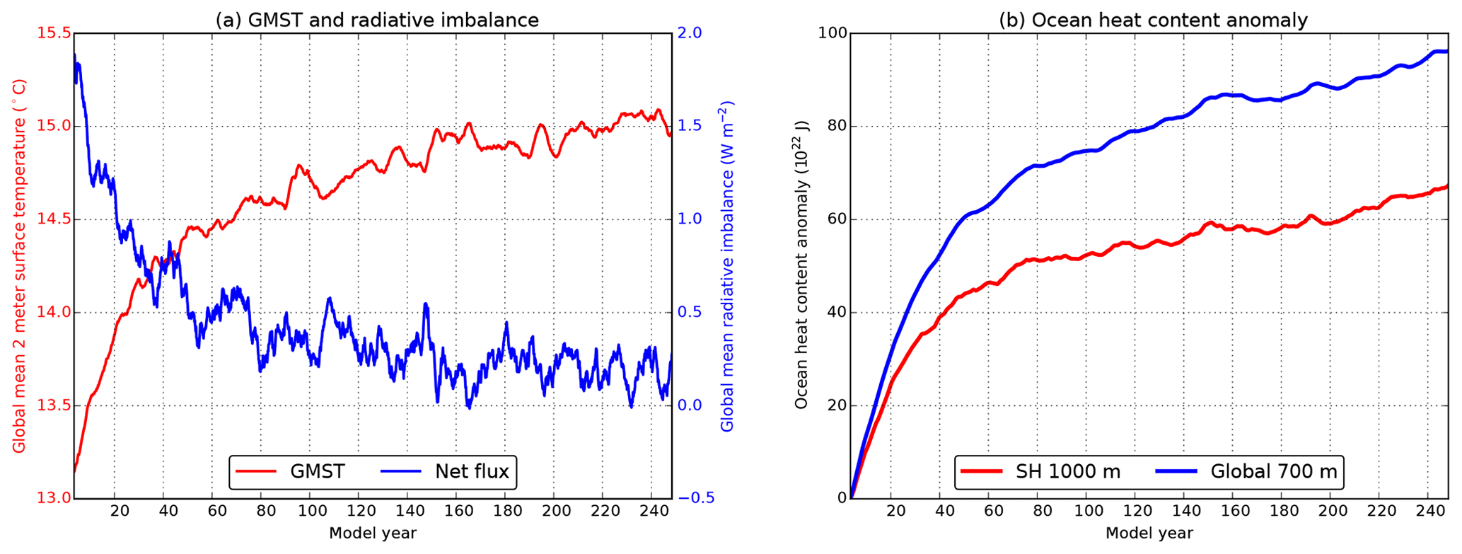
Figure 1Equilibration of the CESM simulation for (a) the global mean 2 m surface temperature (GMST) and global radiative imbalance at the top of the model (net flux) and in (b) the upper 700 m global ocean heat content (OHC) anomaly and the upper 1000 m Southern Hemisphere OHC anomaly. The anomalies are with respect to their initial value of model year 1. All time series are smoothed by a 60-month running mean.
Dufour et al. (2017) analysed MRP events in two versions (eddy-permitting and eddy-resolving) of the GFDL-CM. The lower-resolution version has a weaker vertical background stratification (compared to the high-resolution version) and displays quasi-continuous deep convection events. The effects of eddy-driven heat and salt transport and the representation of overflows were shown to be crucial for the stratification changes in the Maud Rise region (Dufour et al., 2017). In addition, Weijer et al. (2017) demonstrated in a 100-year model simulation of the Community Earth System Model (CESM) that the MRP is only present in the eddying version of the same model. The results in Dufour et al. (2017) and Weijer et al. (2017) suggest that ocean eddies (and also overflows) play a significant role in the vertical background stratification (in addition to the effects already mentioned by Reintges et al., 2017) and therefore affect the timescale of the occurrence of deep convection.
The diverse multidecadal (Reintges et al., 2017) to centennial (Martin et al., 2013) variability found in climate models gives the impression that convection can occur rather randomly through surface density perturbations once the water column is sufficiently preconditioned. However, recently rather regular multidecadal patterns of internal variability have been found in strongly eddying ocean models in the Southern Ocean, the so-called Southern Ocean Mode (SOM; Le Bars et al., 2016). Dynamical processes involving eddy–mean flow interaction and eddy–topography interaction (Hogg and Blundell, 2006) are the driving mechanisms of the SOM (Jüling et al., 2018). Recently, van Westen and Dijkstra (2017) have shown that the SOM variability also occurs in a high-resolution ocean-eddying version of CESM.
In this paper, we pursue the idea of the possible existence of a preferred multidecadal timescale of MRP events in the Southern Ocean through preconditioning and subsequent convection, by analysing the results of an extended CESM simulation as in van Westen and Dijkstra (2017). In this multi-century CESM simulation, several MRP events are found and we analyse the processes involved in these events. In Sect. 2, information on the CESM simulation and mean properties of the (Antarctic) sea-ice field in the simulation are given. As the Southern Ocean Mode is a relatively recent concept, we provide a brief overview and several characteristics of this mode in Sect. 3. Analysis of the MRP events in CESM is provided in Sect. 4. A summary and discussion of the results with the main conclusions are given in the final Sect. 5.
The model output of CESM version 1.0.4 (Hurrell et al., 2013) is taken from the same simulation as used in van Westen and Dijkstra (2017), which has been extended for this study to model year 250. The ocean component (Parallel Ocean Program; POP) and the sea-ice component (Los Alamos Sea Ice Model; CICE) of the model have a 0.1∘ horizontal resolution on a curvilinear, tripolar grid which captures the development and interaction of mesoscale eddies (Hallberg, 2013). The ocean model has 42 non-equidistant depth levels, with the highest vertical resolution near the surface. The atmosphere and land surface components of CESM have a horizontal resolution of 0.5∘, and the atmosphere component has 30 non-equidistant pressure levels. The forcing conditions (e.g. CO2, solar insulation, aerosols) are the observed ones over the year 2000 and are seasonally varying and repeated for every model year.
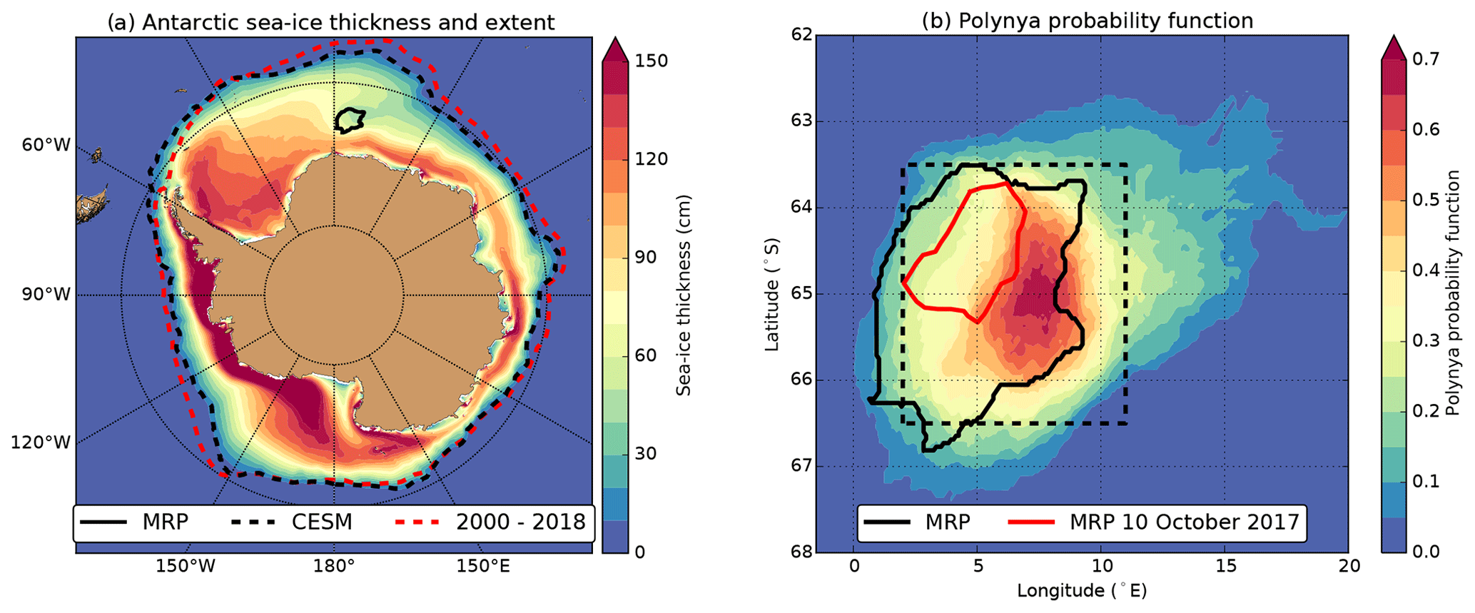
Figure 2(a) Average sea-ice thickness (contours) for September over all the analysed years (model years 150–250) of the CESM output, including the time-mean September sea-ice extent (dashed black curve) and the time-mean (2000–2018) September sea-ice extent for the Scanning Multichannel Microwave Radiometer (SMMR) and Special Sensor Microwave Imager (SSM/I). The September model year 181 MRP is shown by the black contour in panels (a) and (b). (b) Polynya probability function (explained in Sect. 2) based on all the polynya years. The dashed outlined region (66.5–63.5∘ S, 2–11∘ E) is defined as the polynya region. The observed 2017 MRP is indicated by the red contour in panel (b).
The equilibration of the CESM simulation over the first 250 model years is shown in Fig. 1 (these results extend those in van Westen and Dijkstra, 2017). Transient effects dominate the global mean (2 m) surface temperature and global mean radiative imbalance at the top of the atmosphere time series during the first 100 model years (Fig. 1a). These transient effects become smaller after about 150 years as CESM further adjusts to the present-day forcing conditions. The radiative imbalance remains slightly positive (∼ 0.2 W m−2) over the last 100 years of the simulation. The upper 700 m global ocean heat content and upper 1000 m Southern Hemisphere ocean heat content are still adjusting (Fig. 1b), but relatively small trends (compared to the first 100 model years of the simulation) occur over the last 100 years which can easily be removed through a quadratic detrending. The deep ocean fields take a much longer time to equilibrate, and hence the model state is not yet in equilibrium at year 250. Here, we analyse only the last 101 years (model years 150–250) of the simulation, using monthly averaged fields of the high-resolution output on the 0.1∘ × 0.1∘ horizontal grid, instead of the interpolated output used in van Westen and Dijkstra (2017).
The time-mean September sea-ice extent (based on a minimum sea-ice fraction of 15 %) is shown in Fig. 2a as the dashed black curve and the modelled sea-ice extent is slightly lower compared to observations (dashed red curve). The modelled and observed September sea-ice areas vary between 15.8 and 18.4 million km2 (101 model years) and 18.8 and 21.3 million km2 (19 years), respectively. For observations, we used sea-ice measurements by the Scanning Multichannel Microwave Radiometer (SMMR) and Special Sensor Microwave Imager (SSM/I) (https://nsidc.org/data/g02202/versions/3, last access: 8 August 2019; Peng et al., 2013; Meier et al., 2017). The time-mean September sea-ice thickness (colour plot in Fig. 2a) displays relatively small values in the eastern part of the Weddell Sea. In this part of the Weddell Sea, multiple polynyas over Maud Rise appear in CESM; a modelled MRP is shown by the black curve in Fig. 2a. In a companion CESM simulation, with a lower ocean resolution and sea-ice resolution of 1∘, no MRP formation is found over a simulated period of 1300 years (results not shown).
The MRP is defined as the enclosed region within the Antarctic sea-ice pack that has a sea-ice fraction smaller than 15 % (Weijer et al., 2017). The observed 2017 MRP and a CESM modelled MRP are both located over Maud Rise (Fig. 2b). The MRPs found in CESM turn out to be quite localised in space, and to determine that region, we computed a polynya probability density function. First, we define a polynya year to be a year where an MRP appears for at least 3 months. Secondly, at each MRP, the open-water grid cells (bounded by the 15 % sea-ice fraction contour) and sea-ice-covered grid cells are given a label of 1 and 0, respectively. This procedure is applied to each polynya year, so non-polynya years are discarded. Taking the average over all the labelled fields (0 or 1) results in the polynya probability density function as shown in Fig. 2b. There is a small region near 65∘ S, 7.5∘ E, where there is open water for almost all MRPs. Based on the polynya probability density function, we define the polynya region (66.5–63.5∘ S, 2–11∘ E, shown as the dashed outlined region in Fig. 2b).
We determined spatial averages over the polynya region for the temperature, salinity, ocean heat content, sea-ice fraction, sea-ice thickness and the monthly maximum mixed layer depth. The mixed layer depth is defined as the depth at which the interpolated buoyancy gradient matches the maximum buoyancy gradient (this is standard output in CESM; Smith et al., 2010). The local ocean heat content (OHC), indicated by Hk, at model level zk was calculated as
where dzk is the vertical cell length of the model grid at that level. The quantities ρk, Tk and Cp,k are the local density, temperature and heat capacity, respectively. The temperature, salinity and pressure dependency are taken into account when calculating the local density and heat capacity (Millero et al., 1980; Sharqawy et al., 2010). The drift in the integrated OHC over the polynya region (not shown) is smaller compared to that in the time series in Fig. 1b.
The propagation of particles into the polynya region is studied using OceanParcels (Probably A Really Computationally Efficient Lagrangian Simulator, version 2.1.4; Delandmeter and Van Sebille, 2019). In OceanParcels, one can release a set of virtual particles and track their path under the flow using Lagrangian modelling. Particles are passively advected by the time-varying 3-D velocity field from the CESM output, either forward or backward in time. When a particle is released, its age is set to zero. We used a time step of Δt=1 h to update the location of each particle (by linear interpolation of the velocity fields; Delandmeter and Van Sebille, 2019) and the output of each particle (i.e. age, depth, latitude and longitude) is stored every 10 d.
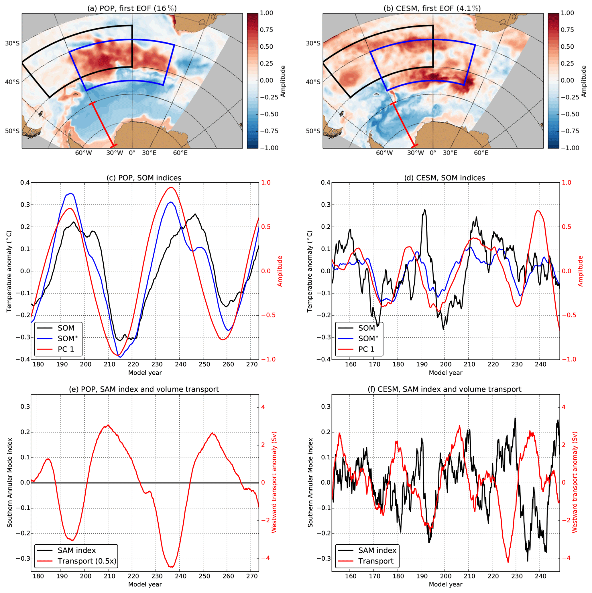
Figure 3(a, b) The first EOF of the upper 1000 m averaged temperature in the Southern Ocean (80–30∘ S, 70∘ W–40∘ E) for the stand-alone POP and for CESM. The black-outlined (blue) region is used to determine the SOM (SOM*) index. The full-depth westward volume transport is determined over the red section (77–60∘ S, 30∘ W). (c, d) The SOM index, SOM* index and the first PC (of the upper 1000 m averaged temperature field) for the stand-alone POP and CESM. (e, f) The SAM index and westward volume transport anomaly at 30∘ W for the stand-alone POP and CESM. The time series in panels (c–f) are quadratically detrended and smoothed with a 60-month running mean. The anomalies of the westward transport are reduced by a factor of 2 for the stand-alone POP.
In a stand-alone ocean simulation with the POP (not to be confused with the coupled model simulation, i.e. CESM), Le Bars et al. (2016) identified a large-scale intrinsic mode of variability in the Southern Ocean (i.e. the SOM). In this simulation, the POP was forced by a yearly repeated and seasonally varying atmosphere where the atmospheric forcing conditions were retained from climatology (see Le Bars et al., 2016 for more details). In Fig. 3a, we show the first empirical orthogonal function (EOF) of the upper 1000 m averaged temperature field for the stand-alone POP (model years 175–275). Each time series of the temperature field was quadratically detrended, the seasonal cycle was removed and then it was normalised by its standard deviation (SD). The resulting time series was then scaled by the area of the grid cell with respect to the largest grid cell area (which is set to 1) and then processed by principle component analysis (PCA; Preisendorfer, 1988). The corresponding principal component (PC) is shown in Fig. 3c (red curve). The first EOF and PC capture 16 % of the total variance and the dominant period of the SOM is 40–50 years (Le Bars et al., 2016; van Westen and Dijkstra, 2017; Jüling et al., 2018).
The variability associated with the SOM can also be measured via the SOM index, which is defined as the surface temperature anomaly over the region 50–35∘ S, 0–50∘ W (Le Bars et al., 2016). The SOM index (also shown in Fig. 3c) displays the same multidecadal variability as the first PC and has a phase difference of about 5 years (65 months) with respect to the first PC. The lag correlation at 65 months is r=0.93 and is significant (95 % confidence interval (CI from now on), taking into account the reduction of the degrees of freedom due to the running mean). The EOF dipole pattern affects the isopycnal slopes in the Southern Ocean (Le Bars et al., 2016) and consequently, via baroclinicity, the Weddell Gyre strength varies with the same period of the SOM (Fig. 3e). The first PC and the Weddell Gyre strength time series are 180∘ out of phase and have a significant (95 % CI) correlation of r = −0.90. The SOM is not related to the SAM (Gong and Wang, 1999) as the SAM index is constant in the stand-alone POP (Fig. 3e).
Applying the same PCA above for the CESM output, we also find a large-scale pattern of variability in the Southern Ocean (Fig. 3b). The dominant period of variability of the first PC is 25 years (Fig. 3d; see also Fig. 5b). The SOM index also displays multidecadal variability in CESM (Fig. 3d) but is much more variable compared to that of the stand-alone POP. For example, the lag correlation between the first PC and the SOM index is much lower in CESM (r=0.47, 95 % CI, 36 months) compared to the stand-alone POP (r=0.93, 95 % CI, 65 months). The differences in the EOF pattern and SOM index between the stand-alone POP and CESM are related to atmospheric and sea-ice processes in CESM. Therefore, we propose the SOM* index, which is defined as the upper 1000 m averaged temperature anomaly over the region of 55–40∘ S, 30∘ W–20∘ E (blue-outlined region in Fig. 3a and b). The SOM* region is based on the maxima of the EOF patterns of both the stand-alone POP and CESM.
The multidecadal variability in CESM is better represented in the SOM* index than in the SOM index (Fig. 3d). For example, from lag-correlation analysis, we find that the first PC is highly correlated with the SOM* index (r=0.80, 95 % CI, 19 months). For the stand-alone POP, the phase difference between the first PC and the SOM* index is 29 months and r=0.95 (95 % CI). Changing the SOM* region (for example, to 50–40∘ S, 0–20∘ E) did not significantly influence the results; it only increases the phase difference between the PC and the SOM* index. The Weddell Gyre strength also varies in the same 25-year period in CESM (Fig. 3f), where the first PC leads by 91 months (r = −0.61, 95 % CI).
Atmospheric and sea-ice-related processes also cause less variance to be captured in the first PC for CESM (4.1 %) compared to the stand-alone POP (16 %). The first and second PCs are well separated for both the stand-alone POP and CESM (North et al., 1982). Still, the variances are rather low in both models. Low variances in PCA are related to spatial noise in large parts of the ocean, the total number of grid cells and the length of the time series. Part of the spatial noise can be removed when the temperature fields are smoothed (through a 60-month running mean) before applying PCA. In this case, the captured variance by the first PC increases to 28.3 % (stand-alone POP) and 15.3 % (CESM). Another possibility to increase the variance is by reducing the region (70–40∘ S, 50∘ W–30∘ E) over which PCA is applied; this results in a variance of 31.3 % and 7.8 % of the first PC for the stand-alone POP and CESM, respectively. Smoothing the time series in this smaller region further increases the variance to 47.1 % (POP) and 23.1 % (CESM). A similar large-scale pattern of multidecadal variability emerges in the first EOF (as in Fig. 3a and b) when reducing the size of the region or by applying a moving average (not shown). To test whether the variances of PCA of the full field are significantly different from red noise (null hypothesis), we generated red-noise surrogate temperature fields with the same statistical properties as the pre-filtered time series. The variance of the first PC of these surrogate temperature fields is 3.8 % and 0.9 % at the 99 % CI (500 surrogate fields) for the stand-alone POP and CESM, respectively. Hence, although the variances of the PCs are relatively small in both the stand-alone POP and CESM, they are significantly different from red noise.
The SAM index (Gong and Wang, 1999) time series in CESM (Fig. 3f) displays interannual variability and does not match with that of the SOM-related multidecadal variability. Lag-correlation analysis of the (smoothed) time series between the first PC and the SAM index did not result in any significant lag correlations. Applying the lag-correlation analysis to the non-smoothed time series, non-significant and low values of lag correlations ( < 0.13) are found between the first PC and the SAM index, as well as between the two SOM indices with the SAM index. Hence, in CESM, atmospheric variability such as the SAM is not related to the large-scale pattern of multidecadal variability associated with the SOM.
Changes in the vertical stratification lead to a different SOM period. van Westen and Dijkstra (2017) found in the first 200 years of the CESM simulation a SOM period of about 40–50 years, which is a similar period to that found in the stand-alone POP of Le Bars et al. (2016). The meridional slope of the isopycnals increases (near 50∘ S) over time in the CESM simulation (not shown), which enhances the baroclinic flow and reduces the period of the SOM. The background density profiles in the CESM output also have a larger meridional isopycnal slope compared to the stand-alone POP (not shown), and hence one would indeed expect a longer period in stand-alone POP compared to CESM. The zonal thermal-wind component near 50∘ S in CESM is about 1.6 times stronger compared to that of the stand-alone POP.
The SOM has not yet been reported in other modelling studies. One of the key features of the SOM is the mesoscale interaction with the background flow (Jüling et al., 2018). As most climate model simulations have a typical horizontal ocean resolution of about 1∘, mesoscale processes are not resolved (Hallberg, 2013), and therefore the SOM mechanism is absent in a non-eddying version of the POP (Le Bars et al., 2016). Moreover, long simulations (> 100 years) are required to develop the SOM in the models. In the first 50 years in the stand-alone POP (model years 75–125), the SOM-related multidecadal variability is much weaker compared to remaining part of the simulation (van Westen and Dijkstra, 2017). For high-resolution models which resolve mesoscale processes (such as in Dufour et al., 2017 and Kurtakoti et al., 2018), the simulated period is too short to develop and/or capture sufficient cycles of the SOM variability.
In Sect. 4.1, we first present the characteristics of the MRP events found in the CESM simulation. It turns out that there is a preferred multidecadal variability in MRP formation, possibly linked to the SOM (Le Bars et al., 2016), and this teleconnection is analysed in Sect. 4.2. The processes causing the associated convective events, in particular the preconditioning of the density field are analysed in the last Sect. 4.3.
4.1 Maud Rise polynyas in CESM
The September sea-ice fraction (blue curve in Fig. 4a) shows relatively low values with respect to the time mean for four periods: model years 158–159, 178–182, 205–209 and 231–237. These relatively low sea-ice fractions (as well as for the sea-ice thickness) are related to polynya formation over Maud Rise. The black curves in Fig. 4b–d represent the annual maximum of the monthly maximum mixed layer depth averaged over the polynya region. During MRP events, the mixed layer depth strongly increases over the polynya region. A deepening of the mixed layer is also strongly correlated (r = −0.98) with a relatively low September sea-ice fraction over Maud Rise.
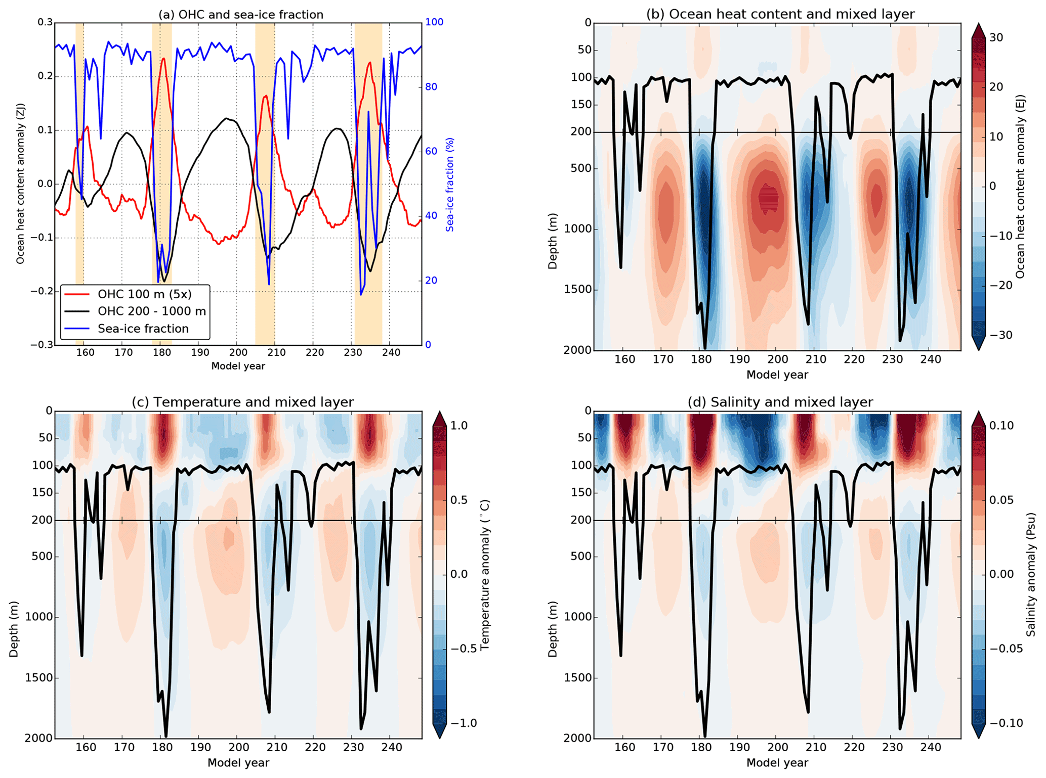
Figure 4(a) Time series of the upper 100 m OHC anomaly (, magnified by a factor of 5), the 200–1000 m OHC anomaly () and the September sea-ice fraction averaged over the polynya region. The OHC time series are quadratically detrended and smoothed by a 60-month running mean. The shading indicates the polynya years. (b) Hovmöller diagram of the OHC anomaly vertical distribution (anomaly of OHC with respect to the time mean) over the polynya region, smoothed by a 60-month running mean. The black curve indicates the annual maximum mixed layer depth. (c, d) Same as panel (b) but now for the oceanic (c) temperature and (d) salinity.
When the mixed layer deepens (i.e. during MRPs), heat and salinity anomalies are mixed towards the surface. The vertical distributions for the OHC, temperature and salinity anomalies over the polynya region are displayed in Fig. 4b–d, respectively. To determine these anomalies at depth zk, first the time mean (over model years 150–250) is subtracted from the time series and the result is quadratically detrended. The resulting time series (Hk, Tk and Sk for heat content, temperature and salinity, respectively) is smoothed using a 60-month moving average. Prior to each multiyear MRP event, positive subsurface (200–2000 m) anomalies of OHC, temperature and salinity are found over the polynya region (Fig. 4b–d, respectively).
On the contrary, the surface layer (upper 100 m) remains relatively cold and fresh prior to polynya formation. This decoupling of the surface and subsurface is also shown in Fig. 3a for and , where we integrated the OHC anomalies over the upper 100 m and between 200 and 1000 m depths, respectively. The time series of and are 180∘ out of phase. During an MRP event, the mixed layer depth increases, positive subsurface heat and salt anomalies are mixed towards the surface, leading to positive surface anomalies there. The surface heat anomalies lead to sea-ice melt and consequently to polynya formation, in agreement with earlier studies (Martin et al., 2013; Dufour et al., 2017; Reintges et al., 2017).
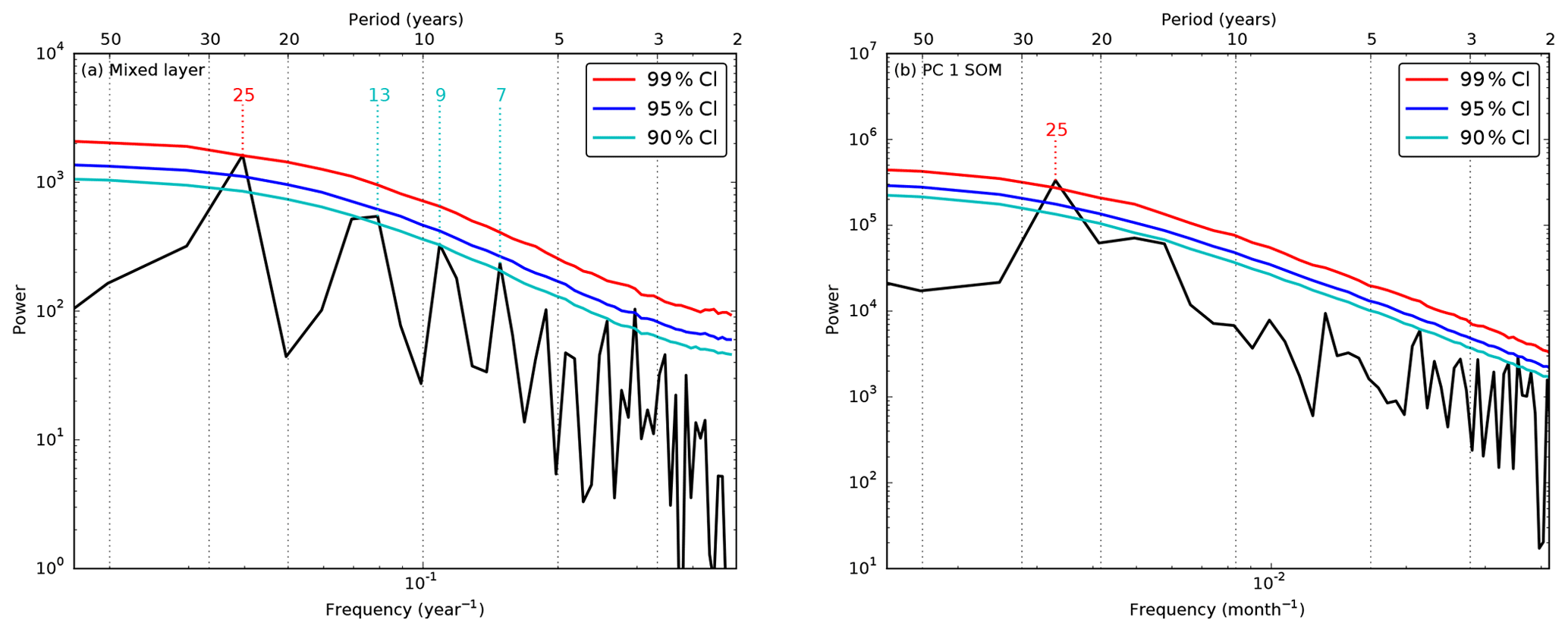
Figure 5Fourier spectrum of the (a) mixed layer depth averaged over the polynya region and (b) the SOM. Before determining the spectrum, the yearly mixed layer depth time series is normalised (to the SD). For the SOM, we retained the non-smoothed first PC time series (see Sect. 3). The confidence intervals (CIs) of significance (99 % (red), 95 % (blue) and 90 % (cyan)) are derived from 10 000 surrogate time series. The indicated periods (in years) are significant at the corresponding colour-coded confidence interval, while only indicating low frequencies (≥ 5 years).
Fourier spectra of the mixed layer depth and the first PC (see Fig. 3d) are shown in Fig. 5. The dominant period of convection (i.e. deepening of the mixed layer depth) has a significant (99 % CI) 25-year period against red noise (Fig. 5a). The time series of OHC, temperature, salinity and sea-ice fraction vary with the same multidecadal period as a consequence of convection (spectra not shown). The first PC also varies on a dominant 25-year period which is significant (99 % CI) against red noise (Fig. 5b). The SOM and SOM* indices also display a dominant multidecadal period (20–30 years; not shown). The possible connection between the SOM and the mixed layer depth variability is analysed in the following section.
4.2 SOM-related variability in the polynya region
As demonstrated in Sect. 4.1, both the SOM and the mixed layer depth over the polynya region display multidecadal variability with the same dominant timescale. In this subsection, the propagation of subsurface heat anomalies towards the polynya region is analysed. For this analysis, we use the SOM* index instead of the first PC because the first PC also contains variability due to MRP formation. The SOM* region is located far outside the polynya region.
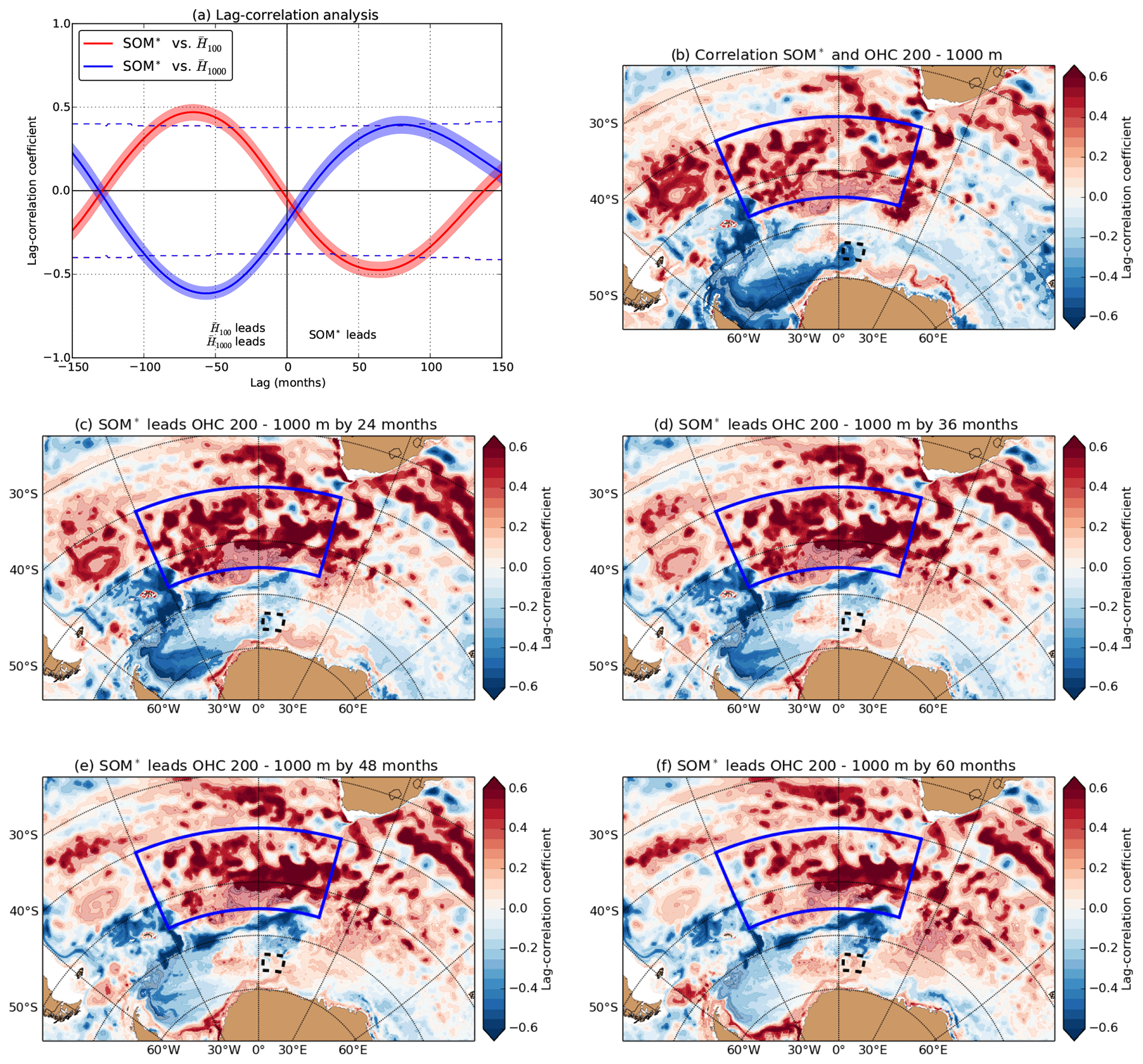
Figure 6(a) Lag-correlation analysis of the SOM* index, the upper 100 m OHC anomaly () and the 200–1000 m OHC anomaly (), averaged over the polynya region (see time series in Figs. 3d and 4a). A positive (negative) lag indicates that the SOM* time series leads (lags) the OHC time series. The shading indicates the 95 % confidence interval of lag correlation, the dashed lines indicate the 95 % significance level. (b) Spatial lag-correlation pattern of the SOM* index time series and the field for zero lag. (c–f) Same as panel (b), but now the SOM* index leads the field by (c) 24, (d) 36, (e) 48 and (f) 60 months. All time series are detrended and smoothed by a 60-month running mean before determining the lag correlation. The blue-outlined region is the SOM* index region and the dashed outlined region the polynya region. The darker coloured correlations indicate significant (95 % CI) lag correlations.
A lag-correlation analysis between the SOM* index (time series in Fig. 3d), and averaged over the polynya region (time series in Fig. 4a) is shown in Fig. 6a. There are significant lag correlations (95 % CI) between the SOM* index and , where the SOM* index leads the by 7 years (80 months). At a similar timescale, negative correlations exists between and the SOM* index. The first PC and the SOM index display similar significant lag correlations with the and averaged over the polynya region.
The lag-correlation patterns of the SOM* index and the field (Fig. 6b and c) at lag 0 and 24 months show overall positive and significant correlations in the South Atlantic, centred around the SOM* region. Positive correlations are propagating along the southern part of the Weddell Gyre towards the polynya region (Fig. 5d–f). The first PC displays similar lag-correlation pattern with the field.
The time-mean flow near the polynya region is westward and is set by the large-scale pattern of the Weddell Gyre (Fig. 7a). Using OceanParcels (see Sect. 2), one can determine the origin of the water mass of Maud Rise. Backtracking the particles (using the time-varying 3-D velocity fields) shows that the particles mainly propagate along the Weddell Gyre and eventually enter the polynya region (Fig. 7b). The particles are initially released at 200 and 500 m depths in the polynya region on December model year 250. One obtains different trajectories when the particles are released in, for example, December model year 249. Therefore, we released particles every 30 d in the polynya region (each spaced by 0.5∘ and fixed initial depth, 133 particles per cast) and we backtracked these particles using OceanParcels over the CESM output (model years 150–250).

Figure 7(a) Time-mean (model years 150–250) and depth-averaged (200–1000 m) horizontal velocity field (arrows), with the speed indicated in the contours. The arrows indicate the direction of the flow (not to scale) and are only shown for speeds larger than 2 cm s−1. (b) The backtracked trajectories for 10 years for some particles (initially spaced at 1∘ × 1∘, 30 particles per initial depth level) which are initially released at 200 m (red curves) and 500 m (blue curves) depths in the polynya region (dashed outlined region).
The backtracked trajectories demonstrate that the particles propagate along the Weddell Gyre and have an upstream origin. Rather than showing all the trajectories (as in Fig. 7b), we show the particle distribution after 7 years (80 months) of backtracking (phase difference between the SOM* index and averaged over the polynya region). The particle distributions are shown in Fig. 8a, c and e, where the particles are initially released at 200, 500 and 1000 m depths in the polynya region, respectively. These results indicate that most particles propagate (backwards) along the Weddell Gyre (similar to the trajectories in Fig. 7b) with little dependence on the initial depth. Note that the final distributions overlap with the positive correlations between the SOM* index and the field (Fig. 6b and c). This implies that when the SOM* index (and also the SOM) is in a positive phase, positive subsurface OHC exists in these parts of the Weddell Gyre. These positive subsurface OHC anomalies propagate along the Weddell Gyre towards Maud Rise in about 7 years.
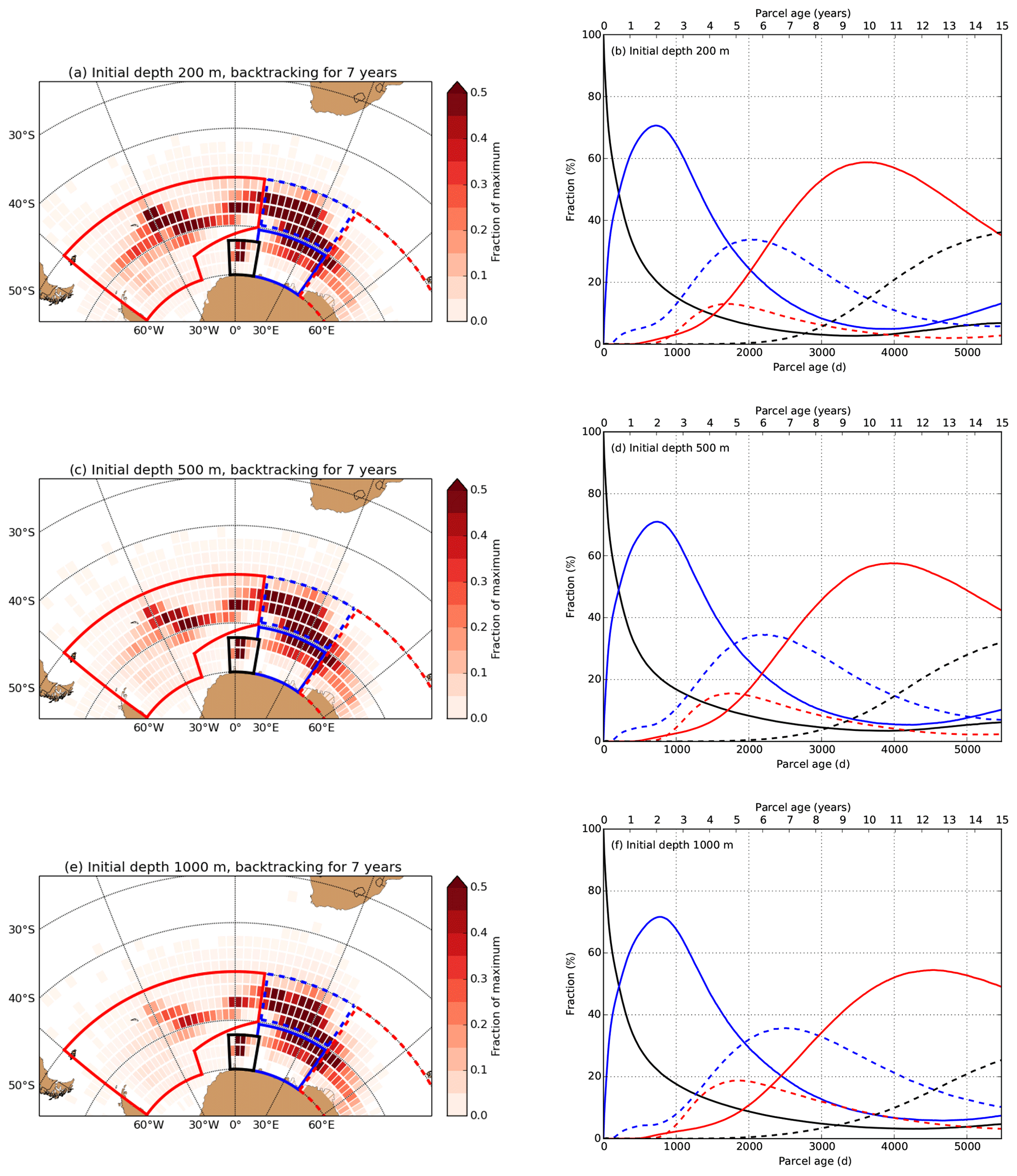
Figure 8(a) Distribution of particles in the Southern Ocean after backtracking the particles for 7 years (80 months). The particles are initiated in the polynya region at 200 m depth every 30 d. The colour-coded regions are used in panel (b), where the dashed red region has a zonal extent of 60∘ (40–100∘ E). (b) The time evolution of the fraction of particles in the colour-coded regions (see panel a). The dashed black curve are particles outside the defined regions. (c–f) Similar to panels (a) and (b), but the particles are initially released at 500 and 1000 m depths in the polynya region.
The backward propagation of the particles along the Weddell Gyre can also be identified using the colour-coded regions (as in Fig. 8a, c and e). Here, we determine the fraction of particles inside a specific region at a given age (Fig. 8b, d and f). All particles are released in the black-outlined region (this region slightly extends the polynya region), and hence all particles have zero age. The time-mean flow in the black-outlined region is directed westwards (Fig. 7a) which explains the relatively high (≈ 70 %) abundance of particles in the blue-outlined region after 2 years of backtracking. Via the dashed blue region, most (> 50 %) particles end up in the red region after about 9–13 years.
The interpretation of these results is that when the SOM is in a positive phase, positive (subsurface) OHC anomalies are found in the SOM* region (Fig. 3b). The SOM* index, which is merely a measure of the phase of the SOM, shows significant correlations with the field and also positive correlations are found in the SOM* region (Fig. 6b). These subsurface OHC anomalies reach the polynya region in about 7 years (Fig. 6d–f). In this way, the subsurface OHC anomalies are advected along the Weddell Gyre and enter the polynya region (Fig. 7 and 8).
4.3 Preconditioning of the polynya region
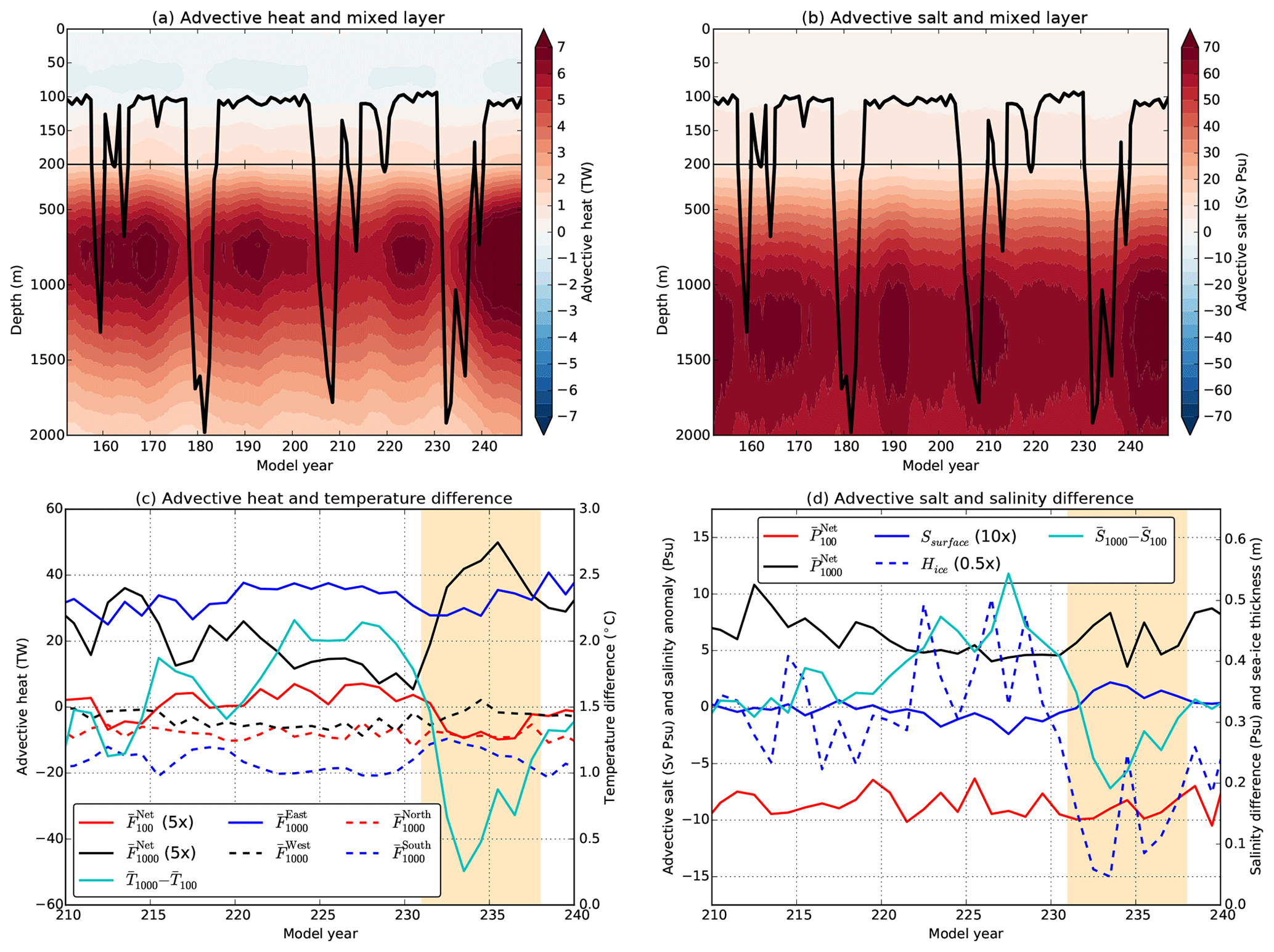
Figure 9(a) Hovmöller diagram of the vertical distribution of heat input along the eastern boundary of the polynya region (63.5–66.5∘ S, 11∘ E). Positive (negative) values indicate heat advected into (out of) the polynya region. The time series are smoothed by a 60-month running mean. The black curve again indicates the (annual maximum) mixed layer depth of the polynya region. (b) Similar to panel (a) but now for the salt input. (c) The horizontal heat input over the polynya region boundaries over model years 210–240, where positive (negative) values of indicate accumulation (depletion) of heat in the polynya region over the corresponding vertical extent. The net horizontal heat input over the polynya region boundaries are indicated by (magnified by a factor of 5) over the corresponding vertical extent. The cyan curve is the temperature difference between subsurface () and surface () over the polynya region. All the time series consist of yearly averages, and the shading indicates the last multiyear MRP event. (d) Similar to panel (c) but now for the net advective salt input ( and ). The cyan curve is the salinity difference between subsurface () and surface () over the polynya region. In addition, the blue curve shows the yearly averaged surface salinity anomaly with respect to model year 210 (Ssurface, magnified by a factor of 10) and the dashed blue curve displays the annual maximum sea-ice thickness (Hice, reduced by a factor of 2).
The propagation of subsurface OHC anomalies associated with the SOM causes subsurface heat accumulation in the polynya region and leads to changes in the subsurface heat reservoir. The horizontal advective heat flux, indicated by Fk, at model level zk, was calculated as
where uk is the horizontal velocity vector at depth zk. The zonal heat input at the eastern boundary () of the polynya region (i.e. the normal component of Fk multiplied by the area perpendicular to the normal) with depth also displays multidecadal variability (Fig. 9a). At mid-level depths, heat is advected into the polynya region with the largest magnitudes occurring at depths between 700 and 900 m. This maximum in heat advection between 700 and 900 m depths is related to the maximum westward velocity which also occurs at subsurface depths. Positive (negative) values of indicate heat advection into (out of) the polynya region.
The subsurface heat reservoir increases when there is net heat input into the polynya region. The development of heat input between 200 and 1000 m depths over the four boundaries (i.e. , , and ) prior to the last multiyear MRP event is shown in Fig. 9c. The net heat input between 200 and 1000 m depths (i.e. sum over the four boundaries, ) is indicated by the black curve in Fig. 9c and the net heat input over the upper 100 m is indicated by (dashed black curve). In addition, the temperature difference between subsurface (, 200–1000 m depths) and surface (, upper 100 m) averaged over the polynya region is shown in Fig. 9c, which is a measure for the magnitude of the subsurface heat reservoir.
In model years 210–215, shortly after the third multiyear MRP event, the heat reservoir is depleted and the temperature difference is relatively small compared to period (model years 225–230) before the 231–237 MRP. Between model years 210 and 230, is positive and larger compared to , leading to an increase in the vertical temperature difference. As the temperature difference increases, the total amount of subsurface heat advected out (sum of , and ) of the polynya region also increases; consequently, the net heat input decreases over time. The time series (model years 150–250) of the temperature difference and are significantly anti-correlated (95 % CI, r = −0.88). The buildup of the subsurface heat reservoir weakens the stratification over the polynya region. During polynya formation, heat is vertically mixed, causing a near-zero temperature difference which indicates that the upper 1000 m is well mixed. Once convection ceases, the temperature difference returns to values of about 1.5 ∘C (which is comparable to the values in model year 210) and the buildup of the heat reservoir starts all over again. Observations prior to the MRP during the years 2016–2017 showed no long-term buildup of a subsurface heat reservoir (Campbell et al., 2019). However, there are observations near Maud Rise, indicating subsurface heat accumulation over longer periods of time (Smedsrud, 2005; Fahrbach et al., 2004, 2011).
Preconditioning of the polynya region also occurs by advection of salinity anomalies into the polynya region, and the advective salt fluxes are given by
The salt input at the eastern boundary () of the polynya region with depth is shown in Fig. 9b. Here, we expressed the salt input in units of Sv psu (1 Sv ≡ 106 m3 s−1), where 1 Sv psu is about 109 g salt s−1. At the eastern boundary, salt is advected into the polynya region over the upper 2000 m and the largest magnitude of salt advection is found between 1000 and 1500 m depths.
The eastern boundary contributes to subsurface salt accumulation in the polynya region (Fig. 9b); the other three boundaries (not shown) advect salt out of the polynya region. The signs of and are opposite, leading to an increase in the salinity difference between the subsurface (, 200–1000 m) and surface (, upper 100 m) over the polynya region prior to MRP formation (Fig. 9d). An increase in the vertical salinity gradient strengthens the stratification of the polynya region. A saline surface layer (due to brine rejection) weakens the stratification, potentially leading to convection (Martinson et al., 1981). Therefore, we determined the surface salinity and sea-ice thickness averaged over the polynya region which are also shown in Fig. 9d. The yearly averaged surface salinity time series is expressed as an anomaly with respect to model year 210. For the sea-ice thickness time series, we retained the annual maximum. Prior to MRP formation, the annual maximum sea-ice thickness was increasing over time, leading to more brine rejection, but this did not result in any increase of the surface salinity over the same period. Taking the average over the months of April–July (i.e. sea-ice growth season) for the surface salinity also results in a decrease of surface salinity values prior to MRP formation. Changes in the vertical salinity gradient are mainly determined by horizontal (sub)surface advection of salt.
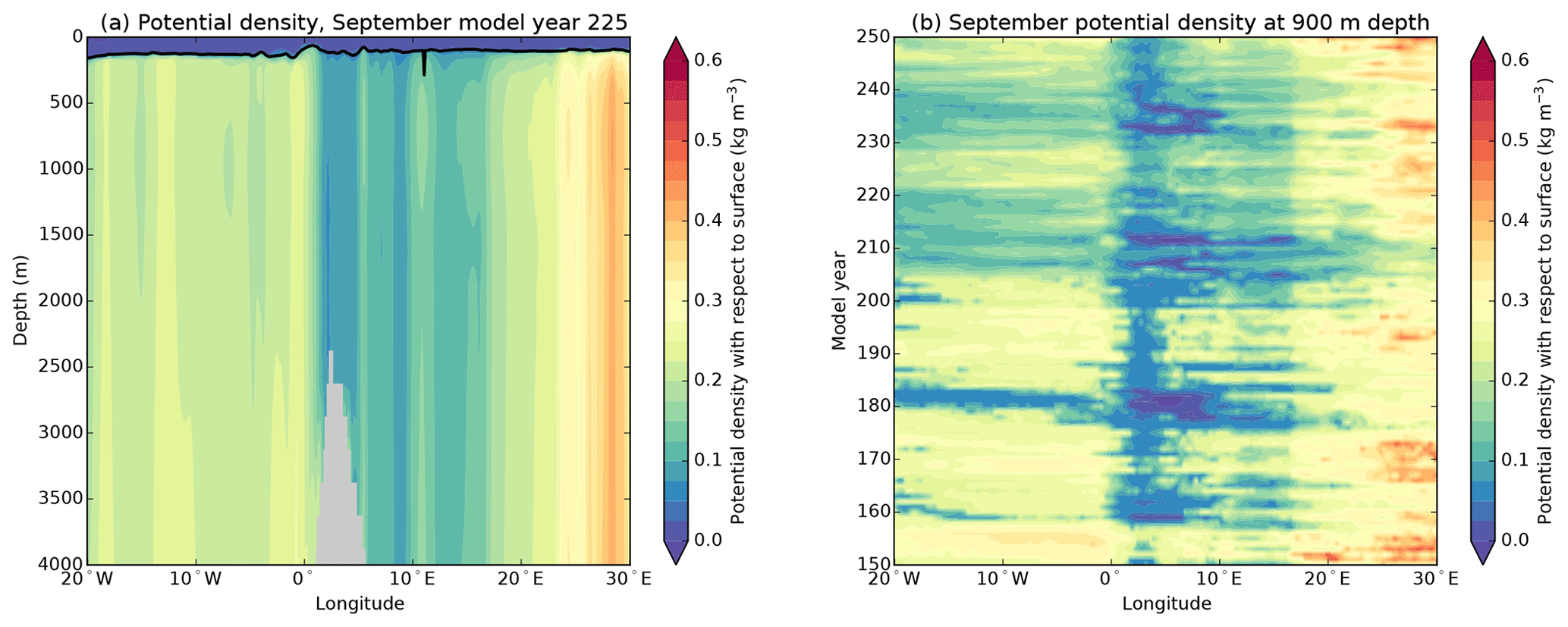
Figure 10(a) Potential density across Maud Rise for September, model year 225. The black curve displays the monthly maximum mixed layer depth of that month. (b) Hovmöller diagram of the September potential density at 900 m depth. The potential density and maximum mixed layer depth are meridionally averaged between 65 and 64∘ S.
Stratified Taylor columns over Maud Rise also contribute to preconditioning of the region (Alverson and Owens, 1996; de Steur et al., 2007). The water column over Maud Rise is weakly stratified compared to the surroundings but there is no (deep) convection prior to MRP formation (Fig. 10a). Here, we determined the potential density (standard output of CESM) and mixed layer depth between 65 and 64∘ S and across 20∘ W–30∘ E; this section crosses the Maud Rise summit (near 3∘ E). There are also Taylor columns over Maud Rise during other years, as shown by the potential density at 900 m depth in Fig. 10b. During the polynya years, the potential density at 900 m depth (as well as for other depth levels) tend to zero over Maud Rise, indicating that the water column overturns. Gordon et al. (2007) suggest that a negative phase of the SAM contributes to the preconditioning of the region; however, the SAM is (strongly) positive before the first (158–159), third (205–209) and fourth (231–237) multiyear MRP events in CESM (Fig. 3f).
Based on this analysis of the CESM results, the preconditioning of the density field seems to be most affected by the subsurface heat anomalies and Taylor columns over Maud Rise. Positive subsurface heat and salt anomalies, advected via the Weddell Gyre, increase the vertical gradient in temperature and salinity over the polynya region, respectively. The increased vertical temperature (salinity) gradient weakens (strengthens) the stratification near Maud Rise.
We analysed the last 100 years of model output from a 250-year control simulation of a high-resolution version of CESM under a repeated seasonal forcing of the year 2000. We find four multiyear MRP events and, in each event, (deep) convection causes vertical mixing of anomalous subsurface heat towards the surface where it melts the sea ice and leads to the formation of the MRP. These processes of the formation and life cycle of the MRP are broadly in agreement with the classical view as in Martinson et al. (1981) and those described from other model results in Martin et al. (2013), Dufour et al. (2017) and Reintges et al. (2017). In most model studies, deep convection occurs rather randomly, while in CESM deep convection occurs about every 25 years.
In CESM, we find that the multidecadal preconditioning of the subsurface density can be linked to an intrinsic dynamical ocean mode in the Southern Ocean, the SOM, which is dominantly caused by eddy–mean flow interaction (Jüling et al., 2018). A positive phase of the SOM leads to positive subsurface OHC anomalies in the South Atlantic Ocean (Le Bars et al., 2016). These anomalies enter the Weddell Gyre near 30∘ E and eventually reach the polynya region, where the anomalies cause deep convection and sea-ice melt. Hence, the frequency of occurrence of the MRP events is related to the SOM variability through the advection of the subsurface OHC anomalies in the Weddell Sea. In this case, a preferred frequency of convective events is induced through preconditioning, which is around 25 years in CESM.
Although preconditioning of the density field in the Maud Rise region is connected to subsurface advection of heat and salt anomalies and Taylor columns, it does not strictly imply polynya formation. However, it will favour the occurrence of MRPs due to atmospheric variability, such as intense winter storms. For example, the formation of the 2016–2017 MRP was initiated by an increased storm frequency under the influence of a positive SAM index (Campbell et al., 2019). In CESM, the SAM index is in a positive phase prior to MRP formation, but the initiation process of the MRPs is out of the scope of this study.
Observations are unfortunately too sparse to falsify the hypothesis of a preferred multidecadal variability in the Southern Ocean. Reanalyses of sea surface temperatures are available to derive a historical SOM index, but the time series is too short to adequately detect the SOM. Relatively low sea-ice fractions were observed over Maud Rise in the mid-1970s, 1980, 1994 and 2016–2017 (Comiso and Gordon, 1987; Lindsay et al., 2004; Gordon et al., 2007; Campbell et al., 2019), suggesting a 15- to 20-year return period of MRP formation which is a bit shorter compared to the 25-year period of the CESM MRPs. The background state of the Southern Ocean sets the reoccurrence time for deep convection (Reintges et al., 2017) which explains the differences in the return period of MRP formation. Besides, the stand-alone POP has a different background state compared to that of CESM, leading to much longer reoccurrence time of deep convection in the stand-alone POP compared to CESM (Jüling et al., 2018). Nonetheless, if the view is correct that a preferred multidecadal frequency (∼ 20 years) in the Southern Ocean exists, it would imply that the next MRP event, if not affected by climate change (De Lavergne et al., 2014), can be expected before the mid-2030s.
Part of the Python (2.7.9) code as well as processed CESM model output can be accessed at https://github.com/RenevanWesten/OS-Multidecadal_Polynya (van Westen and Dijkstra, 2020). The complete model output and analysis scripts are available on request from the corresponding author.
Both authors generated the idea for this study and wrote the paper together. The first author conducted the analysis and prepared all figures.
The authors declare that they have no conflict of interest.
The authors thank Michael Kliphuis (IMAU, UU) for performing the CESM simulations. The computations were performed on the Cartesius at SURFsara in Amsterdam, the Netherlands. Use of the Cartesius computing facilities was sponsored by the Netherlands Organisation for Scientific Research (NWO) under project 15552. The data from the model simulation used in this work are available upon request from the authors. The NOAA/NSIDC provided the satellite sea-ice products. The OceanParcels framework can be obtained online (http://oceanparcels.org, last access: 7 February 2020), and we thank Peter Nooteboom (IMAU, UU) for his assistance in setting up this code for the CESM data.
This research has been supported by the Nederlandse Organisatie voor Wetenschappelijk Onderzoek (grant no. 15552).
This paper was edited by Mario Hoppema and reviewed by two anonymous referees.
Alverson, K. and Owens, W. B.: Topographic preconditioning of open-ocean deep convection, J. Phys. Oceanogr., 26, 2196–2213, 1996. a, b
Campbell, E. C., Wilson, E. A., Moore, G. K., Riser, S. C., Brayton, C. E., Mazloff, M. R., and Talley, L. D.: Antarctic offshore polynyas linked to Southern Hemisphere climate anomalies, Nature, 570, 319–325, 2019. a, b, c, d
Carsey, F.: Microwave observation of the Weddell Polynya, Mon. Weather Rev., 108, 2032–2044, 1980. a, b
Comiso, J. and Gordon, A.: Recurring polynyas over the Cosmonaut Sea and the Maud Rise, J. Geophys. Res.-Oceans, 92, 2819–2833, 1987. a
De Lavergne, C., Palter, J. B., Galbraith, E. D., Bernardello, R., and Marinov, I.: Cessation of deep convection in the open Southern Ocean under anthropogenic climate change, Nat. Clim. Change, 4, 278–282, 2014. a
de Steur, L., Holland, D., Muench, R., and McPhee, M.: The warm-water Halo around Maud Rise: Properties, dynamics and impact, Deep-Sea Res. Pt. I, 54, 871–896, 2007. a, b
Delandmeter, P. and van Sebille, E.: The Parcels v2.0 Lagrangian framework: new field interpolation schemes, Geosci. Model Dev., 12, 3571–3584, https://doi.org/10.5194/gmd-12-3571-2019, 2019. a, b
Dufour, C. O., Morrison, A. K., Griffies, S. M., Frenger, I., Zanowski, H., and Winton, M.: Preconditioning of the Weddell Sea polynya by the ocean mesoscale and dense water overflows, J. Climate, 30, 7719–7737, 2017. a, b, c, d, e, f
Fahrbach, E., Hoppema, M., Rohardt, G., Schröder, M., and Wisotzki, A.: Decadal-scale variations of water mass properties in the deep Weddell Sea, Ocean Dynam., 54, 77–91, 2004. a
Fahrbach, E., Hoppema, M., Rohardt, G., Boebel, O., Klatt, O., and Wisotzki, A.: Warming of deep and abyssal water masses along the Greenwich meridian on decadal time scales: The Weddell gyre as a heat buffer, Deep-Sea Res. Pt. II, 58, 2509–2523, 2011. a
Gong, D. and Wang, S.: Definition of Antarctic oscillation index, Geophys. Res. Lett., 26, 459–462, 1999. a, b
Gordon, A. L.: Deep antarctic convection west of Maud Rise, J. Phys. Oceanogr., 8, 600–612, 1978. a, b
Gordon, A. L., Visbeck, M., and Comiso, J. C.: A possible link between the Weddell Polynya and the Southern Annular Mode, J. Climate, 20, 2558–2571, 2007. a, b, c, d
Hallberg, R.: Using a resolution function to regulate parameterizations of oceanic mesoscale eddy effects, Ocean Model., 72, 92–103, 2013. a, b
Hogg, A. M. C. and Blundell, J. R.: Interdecadal variability of the Southern Ocean, J. Phys. Oceanogr., 36, 1626–1645, 2006. a
Holland, D.: Explaining the Weddell Polynya–a large ocean eddy shed at Maud Rise, Science, 292, 1697–1700, 2001. a, b
Hurrell, J. W., Holland, M. M., Gent, P. R., Ghan, S., Kay, J. E., Kushner, P. J., Lamarque, J.-F., Large, W. G., Lawrence, D., Lindsay, K., Lipscomb, W., H., Long, M. C., Mahowald, N., Marsh, D. R., Neale, R. B., Rasch, P. Vavrus, S., Vertenstein, M., Bader, D., Collins, W. D., Hack, J. J., Kiehl J., and Marshall, S.: The community earth system model: a framework for collaborative research, B. Am. Meteorol. Soc., 94, 1339–1360, 2013. a
Jüling, A., Viebahn, J. P., Drijfhout, S. S., and Dijkstra, H. A.: Energetics of the Southern Ocean Mode, J. Geophys. Res.-Oceans, 123, 9283–9304, 2018. a, b, c, d, e
Kurtakoti, P., Veneziani, M., Stössel, A., and Weijer, W.: Preconditioning and formation of Maud Rise polynyas in a high-resolution Earth system model, J. Climate, 31, 9659–9678, 2018. a, b
Latif, M., Martin, T., Reintges, A., and Park, W.: Southern Ocean Decadal Variability and Predictability, Current Climate Change Reports, 3, 163–173, 2017. a
Le Bars, D., Viebahn, J. P., and Dijkstra, H. A.: A Southern Ocean mode of Multidecadal Variability, Geophys. Res. Lett., 43, 2102–2110, 2016. a, b, c, d, e, f, g, h, i, j
Lindsay, R., Holland, D., and Woodgate, R.: Halo of low ice concentration observed over the Maud Rise seamount, Geophys. Res. Lett., 31, L13302, https://doi.org/10.1029/2004GL019831, 2004. a
Martin, T., Park, W., and Latif, M.: Multi-centennial variability controlled by Southern Ocean convection in the Kiel Climate Model, Clim. Dynam., 40, 2005–2022, 2013. a, b, c, d, e
Martinson, D. G., Killworth, P. D., and Gordon, A. L.: A convective model for the Weddell Polynya, J. Phys. Oceanogr., 11, 466–488, 1981. a, b, c, d
Meier, W., Fetterer, F., Savoie, M., Mallory, S., Duerr, R., and Stroeve, J.: NOAA/NSIDC climate data record of passive microwave sea ice concentration, Version 3, National Snow and Ice Data Center, Boulder, CO, available at: https://nsidc.org/data/g02202/versions/3, (last access: 8 August 2019), 2017. a
Millero, F. J., Chen, C.-T., Bradshaw, A., and Schleicher, K.: A new high pressure equation of state for seawater, Deep-Sea Res., 27, 255–264, 1980. a
North, G. R., Bell, T. L., Cahalan, R. F., and Moeng, F. J.: Sampling errors in the estimation of empirical orthogonal functions, Mon. Weather Rev., 110, 699–706, 1982. a
Parkinson, C. L.: On the development and cause of the Weddell Polynya in a sea ice simulation, J. Phys. Oceanogr., 13, 501–511, 1983. a
Peng, G., Meier, W. N., Scott, D. J., and Savoie, M. H.: A long-term and reproducible passive microwave sea ice concentration data record for climate studies and monitoring, Earth Syst. Sci. Data, 5, 311–318, https://doi.org/10.5194/essd-5-311-2013, 2013. a
Preisendorfer, R. W.: Principal Component Analysis in Meteorology and Oceanography, Elsevier, Amsterdam, the Netherlands, 1988. a
Reintges, A., Martin, T., Latif, M., and Park, W.: Physical controls of Southern Ocean deep-convection variability in CMIP5 models and the Kiel Climate Model, Geophys. Res. Lett., 44, 6951–6958, 2017. a, b, c, d, e, f, g
Sharqawy, M. H., Lienhard, J. H., and Zubair, S. M.: Thermophysical properties of seawater: a review of existing correlations and data, Desalin. Water Treat., 16, 354–380, 2010. a
Smedsrud, L. H.: Warming of the deep water in the Weddell Sea along the Greenwich meridian: 1977–2001, Deep-Sea Res. Pt. I, 52, 241–258, 2005. a
Smith, R., Jones, P., Briegleb, B., Bryan, F., Danabasoglu, G., Dennis, J., Dukowicz, J., Eden, C., Fox-Kemper, B., Gent, P., Hecht, M., Jayne, S., Jochum, M., Large, W., Lindsay, K., Maltrud, M., Norton, N., Peacock, S., Vertenstein, M., and Yeager, S.: The parallel ocean program (POP) reference manual: Ocean component of the community climate system model (CCSM) and community earth system model (CESM), Rep. LAUR-01853, 141, 1–140, 2010. a
van Westen, R. M. and Dijkstra, H. A.: Southern Ocean Origin of Multidecadal Variability in the North Brazil Current, Geophys. Res. Lett., 44, 10540–10548, 2017. a, b, c, d, e, f, g, h
van Westen, R. M. and Dijkstra, H. A.: OS-Multidecadal_Polynya, Github, https://github.com/RenevanWesten/OS-Multidecadal_Polynya, last access: 20 November 2020. a
Weijer, W., Veneziani, M., Stössel, A., Hecht, M. W., Jeffery, N., Jonko, A., Hodos, T., and Wang, H.: Local atmospheric response to an open-ocean polynya in a high-resolution climate model, J. Climate, 30, 1629–1641, 2017. a, b, c, d
Zanowski, H., Hallberg, R., and Sarmiento, J. L.: Abyssal ocean warming and salinification after Weddell Polynyas in the GFDL CM2G coupled climate model, J. Phys. Oceanogr., 45, 2755–2772, 2015. a
Zhang, L. and Delworth, T. L.: Impact of the Antarctic bottom water formation on the Weddell Gyre and its northward propagation characteristics in GFDL CM2.1 model, J. Geophys. Res.-Oceans, 121, 5825–5846, 2016. a