the Creative Commons Attribution 4.0 License.
the Creative Commons Attribution 4.0 License.
 | 13 Nov 2020
Measuring ocean total surface current velocity with the KuROS and KaRADOC airborne near-nadir Doppler radars: a multi-scale analysis in preparation for the SKIM mission
Louis Marié
Fabrice Collard
Frédéric Nouguier
Lucia Pineau-Guillou
Danièle Hauser
François Boy
Stéphane Méric
Peter Sutherland
Charles Peureux
Goulven Monnier
Bertrand Chapron
Adrien Martin
Pierre Dubois
Craig Donlon
Tania Casal
Fabrice Ardhuin
Surface currents are poorly known over most of the world's oceans. Satellite-borne Doppler wave and current scatterometers (DWaCSs) are among the proposed techniques to fill this observation gap. The Sea surface KInematics Multiscale (SKIM) proposal is the first satellite concept built on a DWaCS design at near-nadir angles and was demonstrated to be technically feasible as part of the European Space Agency Earth Explorer program. This article describes preliminary results from a field experiment performed in November 2018 off the French Atlantic coast, with sea states representative of the open ocean and a well-known tide-dominated current regime, as part of the detailed design and feasibility studies for SKIM. This experiment comprised airborne measurements performed using Ku-band and Ka-band Doppler radars looking at the sea surface at near-nadir incidence in a real-aperture mode, i.e., in a geometry and mode similar to that of SKIM, as well as an extensive set of in situ instruments. The Ku-band Radar for Observation of Surfaces (KuROS) airborne radar provided simultaneous measurements of the radar backscatter and Doppler velocity in a side-looking configuration, with a horizontal resolution of about 5 to 10 m along the line of sight and integrated in the perpendicular direction over the real-aperture 3 dB footprint diameter (about 580 m). The Ka-band RADar for Ocean Current (KaRADOC) system, also operating in the side-looking configuration, had a much narrower beam, with a circular footprint only 45 m in diameter. Results are reported for two days with contrasting conditions, a strong breeze on 22 November 2018 (wind speed 11.5 m s−1, Hs 2.6 m) and gentle breeze on 24 November 2018 (wind speed 5.5 m s−1, Hs 1.7 m). The measured line-of-sight velocity signal is analyzed to separate a non-geophysical contribution linked to the aircraft velocity, a geophysical contribution due to the intrinsic motion of surface waves and the desired surface current contribution. The surface wave contribution is found to be well predicted by Kirchhoff scattering theory using as input parameters in situ measurements of the directional spectrum of long waves, complemented by the short wave spectrum of Elfouhaily et al. (1997). It is found to be closely aligned with the wind direction, with small corrections due to the presence of swell. Its norm is found to be weakly variable with wind speed and sea state, quite stable and close to at the Ka band, and more variable and close to at the Ku band. These values are 10 %–20 % smaller than previous theoretical estimates. The directional spread of the short gravity waves is found to have a marked influence on this surface wave contribution. Overall, the results of this study support the feasibility of near-nadir radar Doppler remote sensing of the ocean total surface current velocity (TSCV).
- Article
(18545 KB) - Full-text XML
- BibTeX
- EndNote


The ocean total surface current velocity (TSCV) is defined as the Lagrangian mean velocity at the instantaneous sea surface, corresponding to an effective mass transport velocity at the surface. The TSCV is currently only reliably measured by high-frequency (HF) radars, which are only deployed in some coastal regions. Elsewhere, available estimates depend on numerical model outputs, sea level and wind measurements, and on assumptions such as the balance between the surface pressure gradient and the Coriolis force. The situation is similar regarding directional wave statistics, which are currently mainly estimated through numerical modeling.
These estimates of the TSCV are not reliable at small scales, particularly so in the tropical ocean (e.g., Sudre et al., 2013; Stopa et al., 2016), and these limitations hamper current efforts to observe and understand the fluxes of heat, fresh water, carbon and plastics as well as the coastal impacts of sea states.
Whereas new data on ocean waves are becoming available with the Surface Waves Investigation and Monitoring (SWIM) instrument carried by the China–France Ocean SATellite (CFOSAT) (Hauser et al., 2017, 2020), direct spaceborne measurements of surface current have been limited to a few regions and single projections of the current vector (Chapron et al., 2005; Rouault et al., 2010; Hansen et al., 2011). Several concepts based on SAR (synthetic-aperture radar) interferometry (Romeiser et al., 2003; Buck, 2005) or Doppler scatterometry (Rodriguez, 2018; Chelton et al., 2019) have been proposed for satellite missions aimed at mapping the ocean surface current vector (see review by Ardhuin et al., 2019a). Airborne demonstrators have also been developed in that context (Martin et al., 2018; Rodríguez et al., 2018) and are now becoming operational tools for oceanographic research.
The Doppler frequency shift (DFS) signal provided by these phase-resolving radar instruments is complex: it contains a geophysical contribution due to waves and currents, as well as a large non-geophysical contribution due to the platform motion. The platform velocity in space being of the order of 7 km s−1 for low Earth orbit, it is obviously critical to have accurate knowledge of the measurement geometry to correctly estimate the non-geophysical component. The contribution due to ocean waves is, however, also an order of magnitude larger than the expected TSCV contribution (Nouguier et al., 2018) and must also be precisely estimated using an accurate sea state description.
The Sea surface KInematics Multiscale monitoring (SKIM) satellite mission has been designed to address all these requirements and provide direct global-coverage measurements of TSCV. Its main instrument payload, the SKIM Ka-band Radar (SKaR), a phase-resolved SWIM-like conically scanning radar, provides simultaneous Ka-band observations of sea state and DFS at 6 and 12∘ incidence angles as well as state-of-the-art altimetry observations using a dedicated nadir beam. The nadir beam observations are used to control the SkaR acquisition geometry but are also processed using classical algorithms to provide sea surface elevation, significant wave height and wind speed measurements.
SKIM was preselected as one of the two candidate missions for the European Space Agency (ESA) 9th Earth Explorer. As part of the detailed design and feasibility (phase A) studies, ESA funded a dedicated measurement campaign, Drift4SKIM, which was organized from 21 to 27 November 2018 off the French Atlantic coast, in an area with sea states characteristic of the open ocean and a well-known tide-dominated current regime monitored by a two-site 12 MHz high-frequency radar system (Ardhuin et al., 2009; Sentchev et al., 2013). A range of in situ instruments (surface current drifters, drifting and moored wave-measuring buoys), as well as two airborne Doppler radars operating in the Ku (KuROS – Ku-band Radar for Observation of Surfaces) and Ka (KaRADOC – Ka-band RADar for Ocean Current) bands, were deployed. The campaign goals were to
-
demonstrate how the non-geophysical contribution VNG to the DFS can be estimated from the motion of the platform carrying the radar, the antenna diagram properties, and the azimuth and incidence angle dependencies of the radar cross section;
-
explore the geophysical component VGD and its decomposition as a sum of contributions due to currents and waves, VCD and VWD (Nouguier et al., 2018); and
-
validate the Radar Sensing Satellite Simulator (Nouguier, 2019) and its capability to simulate airborne configurations.
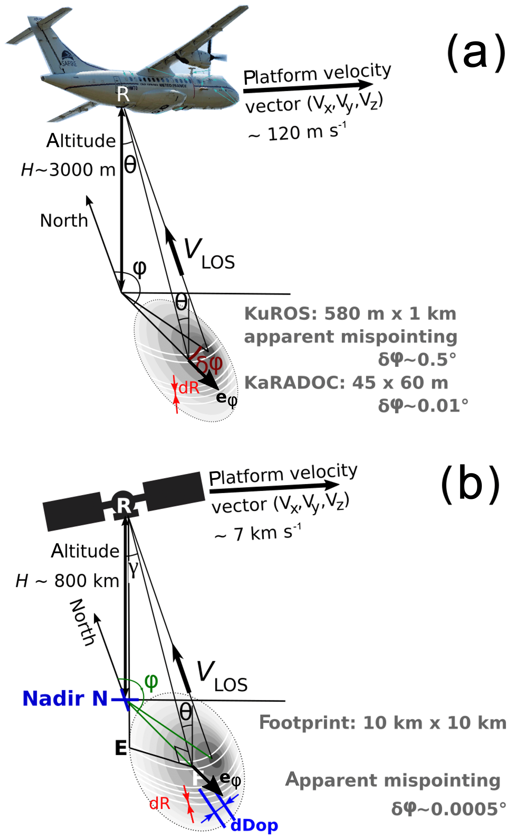
Figure 1(a) Schematic of the ATR-42 aircraft and KuROS instrument with a definition of viewing angles, azimuth φ and incidence angle θ. (b) A comparison with the SKIM viewing geometry. The unit vector eφ is the projection on the horizontal of the line-of-sight direction vector. The variation of surface backscatter across the footprint and as a function of azimuth φ, which causes the effective mispointing δφ, is represented as gray shading. In the KuROS data, each measurement is integrated in azimuth across the antenna lobe. In the case of SKIM, the use of unfocused SAR processing allows for the separation of echoes in the azimuth direction with a resolution of dDop ≃300 m.
As highlighted in Fig. 1, the viewing geometry of an airborne system is vastly different from that of a satellite system, with a much smaller footprint and incidence angle variations at scales comparable to the wavelength of the dominant ocean waves. Another obvious difference is the stability of the platform and its velocity, 7 km s−1 for low Earth orbit and around 120 m s−1 for the ATR-42 aircraft used here. As a result, transposing the performance of an airborne system to a satellite system requires a thorough analysis, supplemented by carefully designed and validated simulation tools. Performing this analysis is, however, worthwhile, as it leads one to develop valuable insight into the instrument imaging principle and design trade-offs.
This article is intended to provide an overview of the Drift4SKIM campaign data and a first discussion of their implications for the emerging field of near-nadir Doppler radar observations of TSCV. It is structured as follows: the principle of the pulse-pair measurements and the different contributions to the observed DFS are detailed in Sect. 2 and Appendix A. Section 3 gives a brief account of the fieldwork performed and conditions encountered during the campaign. The results of the airborne measurements are presented in Sect. 4. Results and implications for SKIM are then discussed in Sect. 5. Conclusions and perspectives follow in Sect. 6.
Shipborne Doppler measurements of ocean currents are routinely performed using so-called vessel-mounted acoustic Doppler current profilers (VMADCPs; see, for instance, Rossby et al., 2019). Some of the data processing concepts transpose directly to the spaceborne context: the raw DFS signal contains a large non-geophysical contribution due to the platform motion, which must be estimated from ancillary sensors and compensated for. The accuracy of the final geophysical product is practically set by the accuracy of the non-geophysical velocity estimation and correction procedure. In the VMADCP context, however, the backscattering elements responsible for the production of the acoustic return signal (particulate suspended matter, zooplanktonic organisms) are passive and accurately follow the water mass. This does not carry over in the electromagnetic case: here, the return signal is produced by the interaction of the transmitted signal with the roughness elements of the sea surface, which move with respect to the water mass with an intrinsic phase velocity that is an order of magnitude larger than typical ocean currents. This effect is, for instance, well known in the ground-based HF radar current measurement context (Stewart and Joy, 1974) and must also be compensated for.
In our case, the measurement geometry is represented in Fig. 1, and the line-of-sight Doppler velocity VLOS looking towards incidence angle θ and azimuth φ (in this paper, line-of-sight DV contributions are denoted by V, and the corresponding horizontal velocity contributions are denoted by U) is the sum of the projection of a horizontal current contribution UCD(φ), a wave-induced contribution VWD(θ,φ) and a non-geophysical contribution VNG(θ,φ). The equation that permits the retrieval of the TSCV contribution UCD(φ) from the raw measured VLOS can be written as
The aim of this section is to provide a detailed analysis of the different terms of this expression. The non-geophysical contribution VNG is discussed in Sect. 2.1 and Appendix A. The wave Doppler contribution is discussed in Sect. 2.2. A brief summary of the measurement error budget is finally provided in Sect. 2.3.
2.1 Non-geophysical velocity VNG
As mentioned above, the accuracy of shipborne acoustic Doppler current measurements is affected in a dominant way by the platform motion compensation process. In the spaceborne context, the platform velocity is almost 3 orders of magnitude larger (7000 m s−1 vs. 10 m s−1 for shipborne measurements). Thus, the accuracy requirements are tremendously exacerbated. In particular, attention must be paid to the detailed effects of the antenna radiation diagram and the sea surface normalized radar cross section (NRCS) variations with space and observation azimuth. A detailed discussion of these effects is given in Appendix A.
In summary, in the case of a sufficiently narrow radiation diagram, VNG can be approximated as the radar carrier velocity projected on an effective look direction. This effective look direction differs from the geometric boresight direction by an effective azimuthal mispointing δφ due to the finite antenna beamwidth combined with the variations of NRCS within the radar footprint, as well as by an effective incidence angle mispointing δθ due to radar timing or surface-tracking errors.
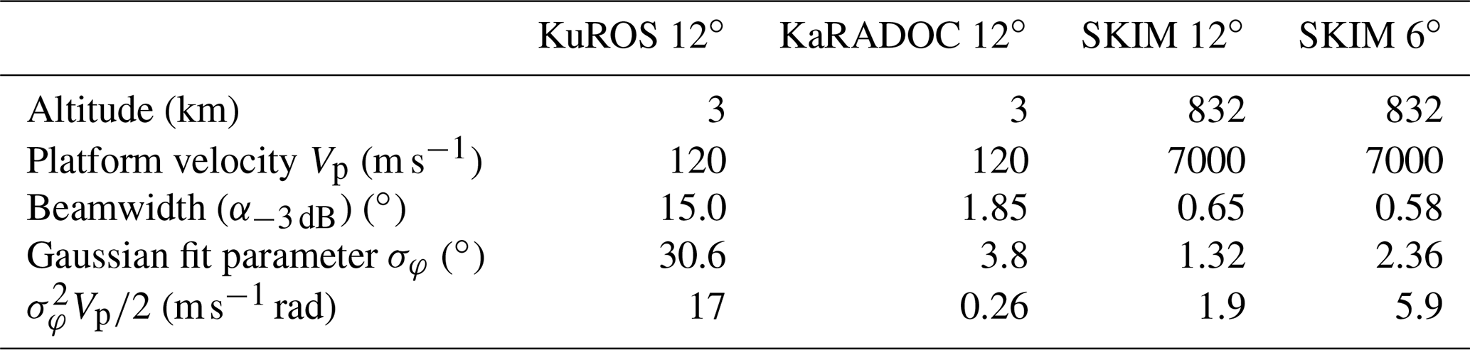
Table 1KuROS and KaRADOC antenna radiation diagram characteristics. All angles are in degrees. See Appendix B for the definitions of α and β.
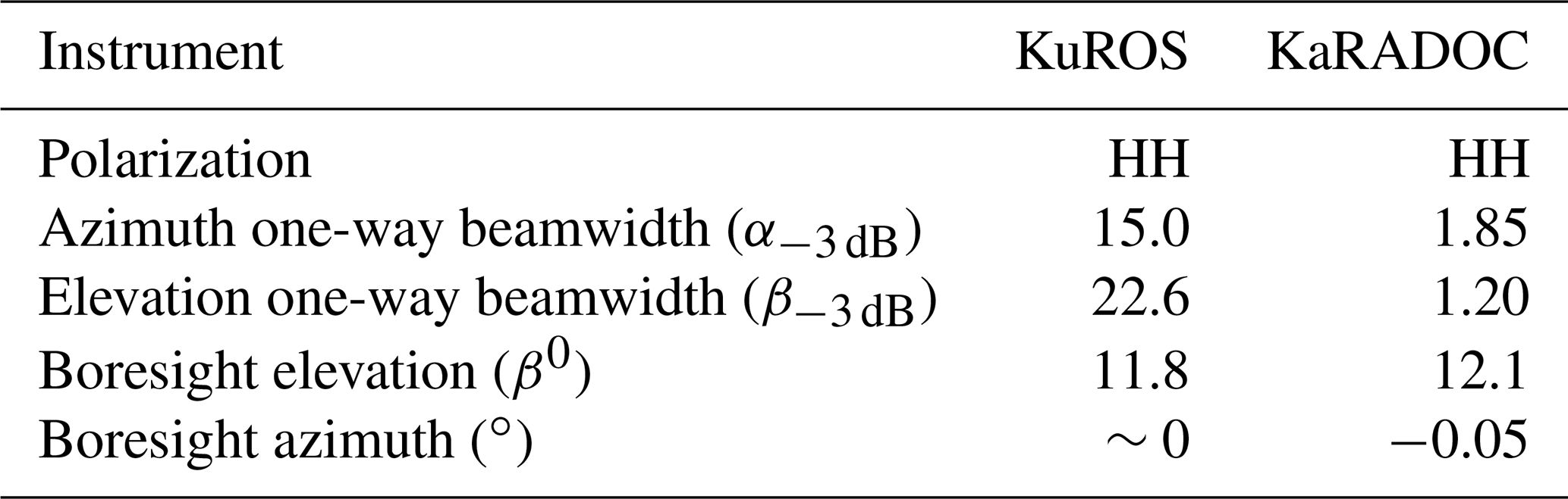
The beamwidth at the working incidence angle is thus a very important parameter of a radar intended for TSCV measurements. Table 1 summarizes the parameters of the KuROS and KaRADOC antennas. For KuROS they have been determined following the procedure detailed in Appendix B. For KaRADOC, they are the result of anechoic chamber measurements (Appendix C). As discussed in Appendix B, these parameters describe the antenna radiation diagrams when expressed as functions of variables, α and β, which do not coincide with azimuth and incidence angle. In the case of constant-altitude flight and near-nadir observations with the antenna looking towards azimuth φb, one can, however, obtain a Gaussian approximation of the one-way radiation diagram as
where and For 12∘ observations the second term in the exponential can safely be neglected, and the effective azimuthal beamwidth can be estimated as
When projected on the ground, φ−3 dB is thus larger than α−3 dB by a factor 1∕sin (θ), equal to 4.8 for 12∘ measurements. Provided that the beam is not too wide, the Gaussian approximation in Eq. (A29) of G as a function of φ can then be used with the parameter
Due to the width of the azimuthal aperture, the NRCS-weighted line-of-sight azimuth φa can differ from the boresight azimuth φb by a mispointing angle δφ. Expressions for δφ are obtained in Appendix A in the two limiting cases of slow linear and fast sinusoidal variations of the ocean surface NRCS with respect to azimuth. In the slow variation case, δφ is obtained as
Denoting by φt the flight track azimuth and Vp the along-track flight velocity, the spurious azimuth gradient Doppler (AGD) contribution to the DV caused by the mispointing reads
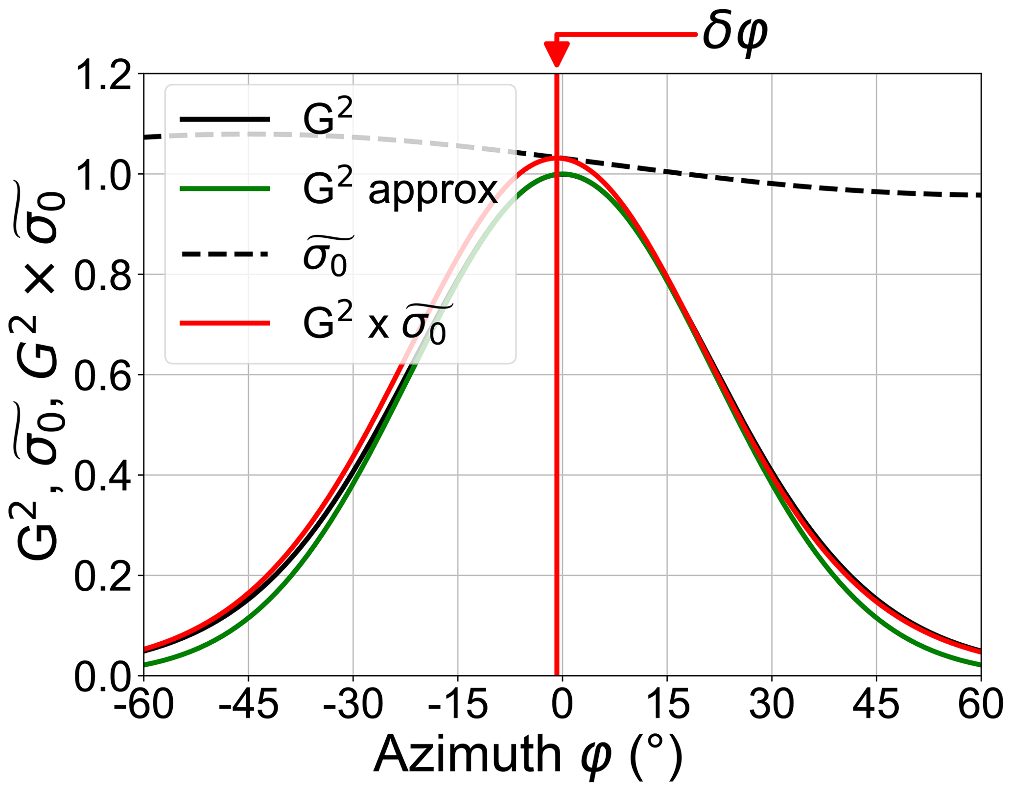
Figure 2KuROS azimuth integral weight at for a north-facing () antenna (black), Gaussian approximation (Eq. A29) (green) and variation of for a typical 11 m s−1 wind from 140∘ (dashed black). The peak of the product (red) is shifted with respect to the peak of G2 by .
As an example, Fig. 2 shows the variations of the two-way antenna radiation diagram G2, its Gaussian approximation and the (see Eq. A11) product as a function of azimuth at a 12∘ incidence angle for a northward-looking KuROS antenna (), using σ0 data from the Drift4SKIM campaign on 22 November 2018. The effect of the wind-induced azimuthal gradient of σ0 is to shift the effective radiation diagram towards the brighter upwind and downwind directions, with an apparent pointing azimuth φa. The shift induced in this case is . For comparison (see Sect. 2.3 and Table 2), the pointing accuracy required to achieve a 15 cm s−1 error on the horizontal current in the airborne configuration is 1.2 mrad.
Here, it is important to note that KuROS was not specifically designed for this experiment but primarily as a calibration and validation instrument for the CFOSAT mission, which required a broad radiation diagram. Though the analysis of the KuROS data helped uncover many interesting effects relevant to Doppler observations of the sea surface, its design was not fully appropriate to validate the inversion of the geophysical velocities, for which the pencil-beam antenna diagram of KaRADOC was better suited.
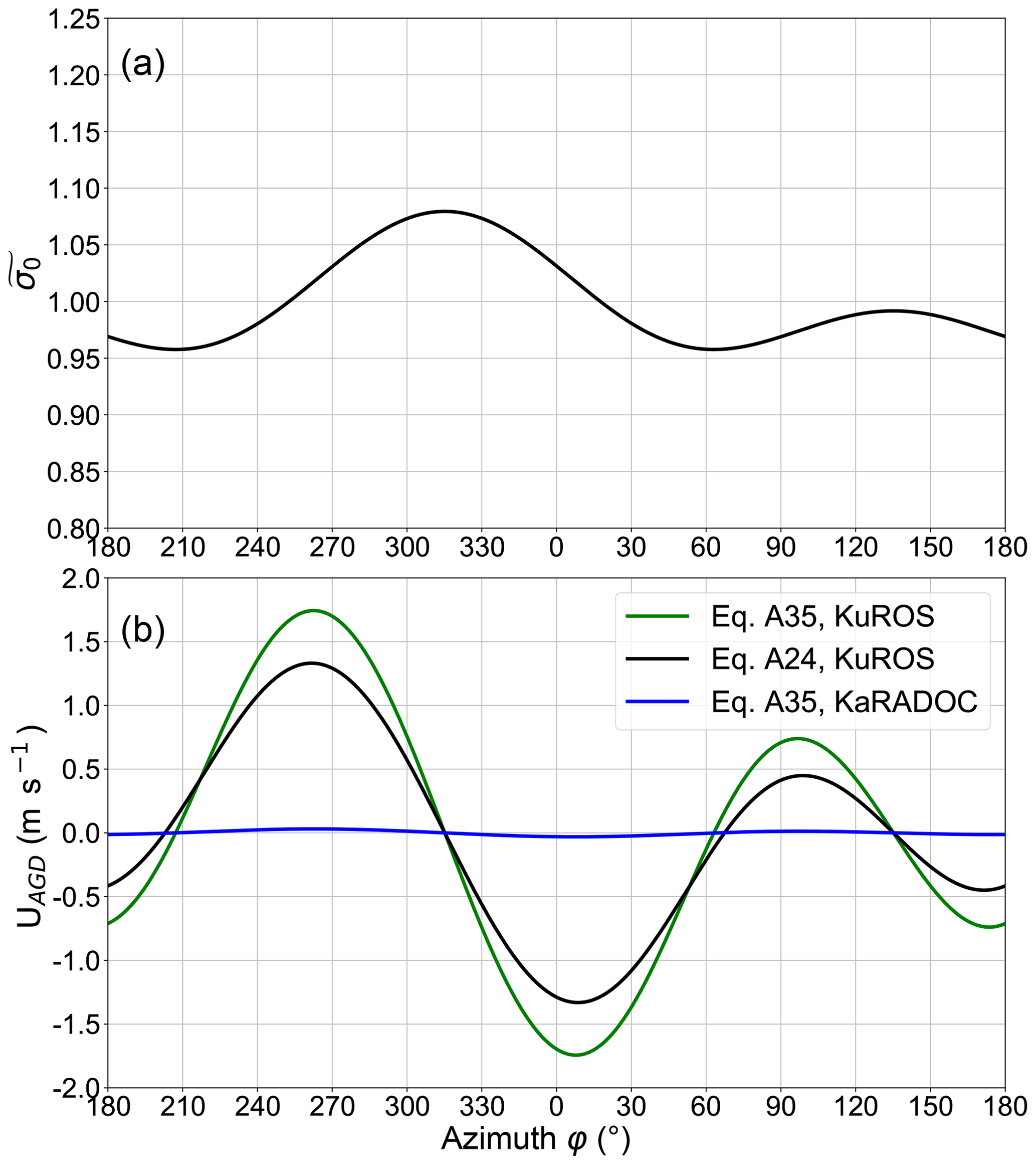
Figure 3(a) Example of azimuthal variation of at a 12∘ incidence angle, corresponding to the 22 November case (11 m s−1 wind from 140∘) discussed in Sect. 3, and (b) associated spurious velocity UAGD as a function of look azimuth φb in the case of a port-looking antenna mounted on a platform in constant-altitude flight at 120 m s−1. For the KuROS case, the green line shows the result of the approximation in Eq. (A35), and the black line shows the result of the full azimuthal integration in Eq. (A24). The blue line represents the result of Eq. (A35) for KaRADOC using the same as in the Ku-band case.
Figure 3a shows a typical example of the azimuthal variation of at a 12∘ incidence angle for the Ku band. As expected for near-nadir measurements (Chapron et al., 2002; Munk, 2008; Chu et al., 2012), the NRCS is largest in the downwind look direction (), has a secondary peak in the upwind direction and is weakest in the crosswind look directions. Figure 3b shows the corresponding UAGD contribution for the KuROS and KaRADOC cases using an aircraft velocity and the Ku-band NRCS fit for both instruments (this is a reasonable assumption for order-of-magnitude estimates). As detailed in Appendix A, Eqs. (5) and (6) only apply for a narrow beam when projected on the ground, which is not a very good approximation for the KuROS case, even at a 12∘ incidence angle. As shown in Fig. 2, the Gaussian approximation for the antenna diagram as a function of φ gives a distribution that is too narrow and does not properly take into account the azimuthal integration, leading to an overestimation of UAGD. It is clear, however, that even the more exact Eq. (A24) gives very large correction magnitudes, in excess of 1.2 m s−1 in some azimuth ranges.
Because the azimuth gradient UAGD contribution to the observed DV is proportional to , this effect is much larger (and correcting it is correspondingly more demanding in terms of antenna characterization) for KuROS than for KaRADOC or DopplerScatt (Rodríguez et al., 2018) thanks to their narrow azimuthal beam aperture. Another remark is that the approximate expression in Eq. (A35), though it gives the appropriate dependency of UAGD with respect to look azimuth, tends to overpredict its magnitude as the widening associated with the ground projection saturates for broad beams.
Although the relative variations are larger for larger incidence angles, this is more than compensated for by the 1∕sin 2θ reduction in azimuthal diversity across the footprint. This effect can thus be neglected for much higher incidence angles (Rodríguez et al., 2018).
2.2 Geophysical velocity UGD: waves and current Doppler velocities
The geophysical part of the DFS measured by a microwave radar over the ocean, using both along-track interferometry and Doppler centroid techniques, emerges from the average over the instrument field of view (FOV) of the backscatter-weighted line-of-sight projection of the surface velocity, as illustrated in Fig. 4.
In the well-understood case of decametric electromagnetic waves interacting with the sea surface at grazing incidence, the interaction is dominated by the Bragg coherent backscattering mechanism (Crombie, 1955), in which the backscattered field reflects the properties (amplitude, phase speed) of a very finely selected component of the sea state, namely that whose wave vector is precisely equal to the so-called Ewald vector, the difference between the wave vectors of the scattered and incident electromagnetic waves. Exploiting the deviation of the phase speed of this sea state component from its theoretical value is the principle of the HF radars operationally used to measure ocean TSCV in coastal areas (Barrick et al., 1974; Stewart and Joy, 1974).
In the case of the near-nadir interaction of microwaves with the sea surface, which is the configuration considered for SKIM and used by the AirSWOT, KuROS and KaRADOC airborne instruments, this mental picture must be adapted: the Bragg scattering mechanism is not dominant, and the main contribution comes from quasi-specular reflections on those facets of the sea surface which are normal to the Ewald vector. The backscattering cross section of the sea surface and DFS in this case do not depend on the properties of a single Fourier component of the sea state but on the probability density function of the sea surface slope, which is a complex functional of its entire directional spectrum.
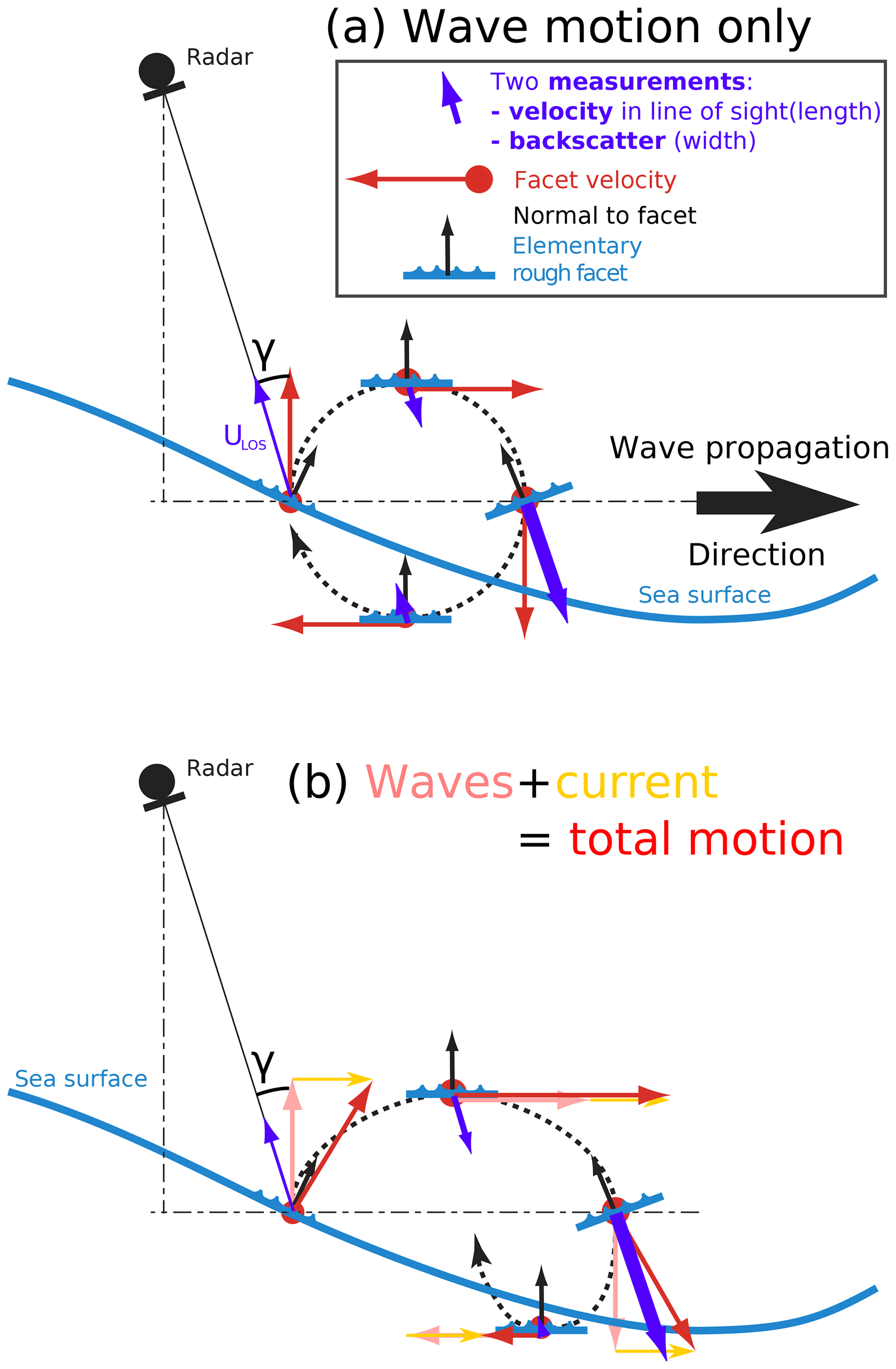
Figure 4Schematic of (a) wave and (b) wave and current contributions to Doppler velocities at the scale of elementary facets. These small-scale processes are averaged over the radar field of view, and a mean velocity signal emerges due to the correlation of surface brightness and velocities in the wave field.
As discussed by Nouguier et al. (2018), who applied it to the analysis of AirSWOT NRCS and DFS data collected during the Gulf of Mexico LASER experiment in 2016, the theoretical framework appropriate for this configuration is the Kirchhoff approximation (Beckmann and Spizzichino, 1987). In this approximation, the geophysical DFS ωGD can be expressed as
where C(τ) is the temporal covariance function of the ensemble-averaged electromagnetic field backscattered in the direction of the radar.
Assuming Gaussian statistics for the sea surface, introducing , the space–time covariance function of the sea surface elevation, and and , the horizontal and vertical components of the Ewald vector (with λ the radar wavelength), one obtains C(τ) and ∂τC as
The clear upwind–downwind asymmetry of σ0 observed in the Drift4SKIM radar observations (see Fig. 10) shows that the Gaussian assumption, which is unable to describe such skewness-related effects, is clearly questionable. It is, however, the only practical option, as going further would require prescriptions for the higher-order statistics of the sea surface, which are at present not available.
The occurrence of ρ as the argument of an exponential in these integrals renders further analytical progress difficult (see, however, Nouguier et al., 2011). Approximate expressions can, however, be obtained by performing a Taylor expansion of ρ in the neighborhood of the origin. This results in a Gaussian approximation of the integrand. The integrals can be readily evaluated, yielding (denoting by “⋅” the usual matrix product)
The derivatives of ρ are taken at ξ=0 and τ=0, and they can be expressed as moments of the directional sea state spectrum Sd(k) as
where, in the notation of Nouguier et al. (2018), msv stands for the mean slope velocity and Mss for the mean square slope matrix,
with
The surface current enters through its effect on the dispersion relation of surface waves ω(k). In the presence of a vertically homogeneous current U (a detailed discussion of the effect of shear can be found in Kirby and Chen, 1989),
where
is the dispersion relation of gravity–capillary waves in deep water, with k the wave vector and the wavenumber corresponding to the gravity–capillary regime transition. Introducing this expression in Eq. (10), and defining msv0 as the spectral moment obtained using the dispersion relation of Eq. (15) in Eq. (13), one obtains the approximate DFS as
and the corresponding VGD as
While clearly oversimplified (it is, for instance, independent of the electromagnetic wavelength, which is known to have a significant influence on σ0), this expression has a definite pedagogical interest, as it allows one to distinguish a number of interesting features.
-
The raw velocity projection VGD accessible to Doppler radar instruments is composed of a “genuine” current Doppler (CD) component VCD, equal to the projection of the TSCV along the radar line of sight, plus a wave Doppler (WD) component VWD induced by the natural motion of the sea surface.
-
This VWD component involves sea surface statistics of two different natures: the mean slope velocity vector msv0 and the mean squared slope matrix Mss. To this order of approximation it can be seen as the projection along the radar line of sight of the constant vector . In the rest of this article, MWD denotes the norm of this vector.
-
As noted in Nouguier et al. (2018), msv0 is equal to one-half the surface Stokes drift velocity of deepwater waves . As noted in Nouguier et al. (2016), the effective mean squared slope matrix Mss components (mssshape), accounting for the electromagnetic filtering effect and part of the non-Gaussianity of the sea surface statistics, can be obtained from the derivatives of σ0 as a function of incidence angle for different azimuths.
-
In simple cases represented by parametric spectral forms such as the Elfouhaily et al. (1997) spectrum used in this work, msv0 and the eigenvectors of Mss are aligned with the downwind direction, and the relation proposed in Chapron et al. (2005) is recovered, with .
-
Both these statistics are, however, known to be influenced by waves at all scales. The asymptotic behaviors of the weighting factors as functions of the surface wave wavenumber in the gravity wave range are k3∕2 and k2 for the msv0 and Mss terms, respectively, while the parametric spectrum of Elfouhaily et al. (1997), used in this work, decays as k−3, leading to a logarithmic divergence for the Mss components and a slow convergence of the msv0 components at high wavenumbers.
-
The Mss components are sensitive to the detailed shape of the spectrum up until the short capillary wave roll-off or to the electromagnetic cutoff, whichever is reached first.
-
Estimating these terms requires knowledge of all the components of the sea state: the long gravity wave range can be measured (either in situ, as during the Drift4SKIM campaign, or using the radar measurements themselves as intended in the SKIM context), but the high-wavenumber range cannot be neglected, and its effect must be accounted for, for instance, through the use of a parametric spectral form.
-
The msv0 vector appears as a multiplicative factor, to which the inverse of the Mss matrix is applied. These terms thus have opposing influences on the final result: modifications of the sea spectrum, which tend to increase the weight of small-scale components, increase the mean slope velocity but also, and rather more, the mean squared slope by which it is divided. A certain degree of stability of the end result is thus likely.
-
On a similarly reassuring note, whereas the low-wavenumber part of the spectrum is affected by swell systems of remote origin that have arbitrary orientations, the short waves represented by the parametric tail of the spectrum are known to be aligned with the wind direction and to depend on local variables only (wind strength and direction, fetch).
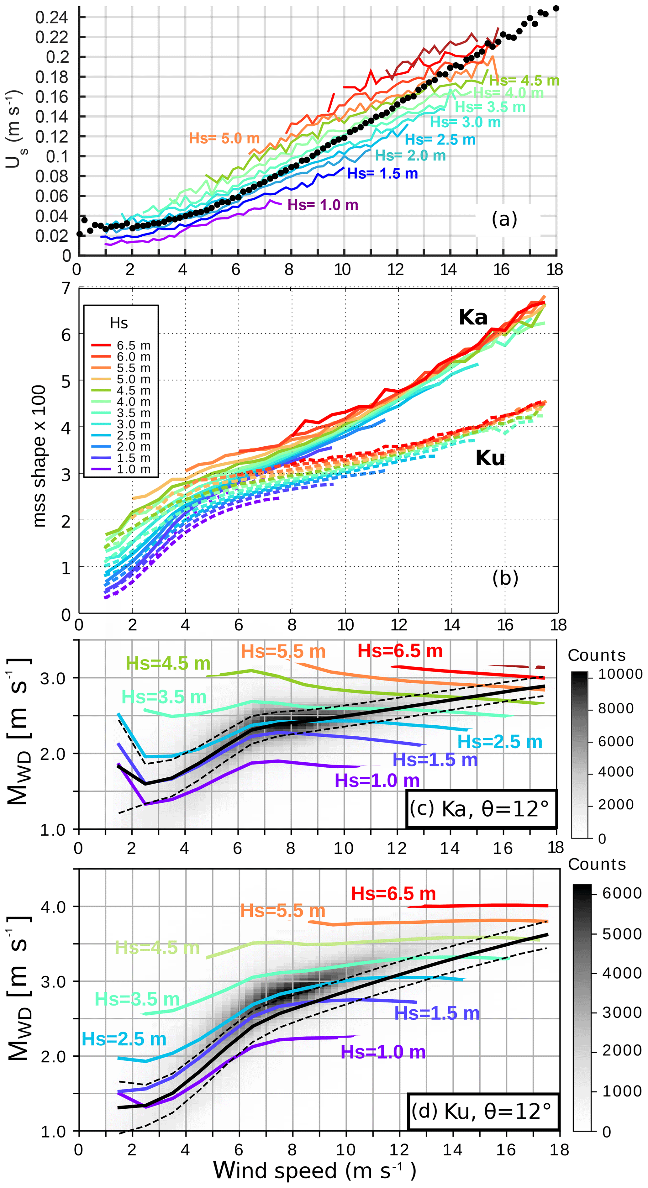
Figure 5Computed variability of the Stokes drift velocity, the diffraction-effective mean square slope mssshape and the wave Doppler velocity magnitude MWD. (a) 2010–2017 statistics of Stokes drift magnitude at Ocean Station Papa, computed using the buoy wind speed data and wave data from the nearby WMO buoy 46 246, maintained by the University of Washington (Thomson et al., 2013). (b) mssshape estimated from GPM satellite backscatter using modeled co-located wind speed and wave height; reproduced from Nouguier et al. (2018). (c, d) Statistics of the Ka- and Ku-band MWD, computed using the theoretical model of Nouguier et al. (2011) for ocean wave spectra modeled over the global ocean using the WAVEWATCH III model (Stopa et al., 2016) and plotted as a function of the wind speed. The colored curves show the median value for different classes of wave height for a given wind speed; each curve is separated by 0.5 m in panels (a) and (b) and by 1 m in panels (c) and (d). In (c) and (d), the gray shading represents the histogram of the computed MWD values in the global simulation.
Figure 5 gives orders of magnitude for the natural range of variability of the different factors thus isolated. Figure 5a shows the variability of the Stokes drift velocity estimated following Kenyon (1969) and Ardhuin et al. (2009) using wind and directional wave measurements collected from 2010 to 2017 at Ocean Station Papa. Even though US is highly correlated with the wind speed with a Pearson's linear correlation coefficient of 0.85, a strong dependence on the long-wavelength part of the spectrum, for which Hs is a proxy, definitely has to be accounted for.
Figure 5b, taken from Nouguier et al. (2016), instead shows the dependence on wind speed and Hs of Ku- and Ka-band effective mean squared slope mssshape retrieved from the GPM (Global Precipitation Mission) satellite measurements. The variability is even more strongly dominated by the dependence on wind speed, the variability due to the long-wavelength part of the spectrum being much smaller. These measurements very clearly show the filtering effect of the electromagnetic wavelength and are a clear warning that Eq. (17), suggestive though it is, should be considered with caution.
Finally, Fig. 5c and d show the magnitude of the horizontal UWD component as a function of wind speed and Hs, estimated by numerically evaluating the integrals of Eqs. (8) and (9) for C(τ) and ∂τC using the numerical tools of Nouguier et al. (2011) on the basis of long-wavelength spectra extracted from global runs of the WAVEWATCH III model (Stopa et al., 2016), completed in the high-wavenumber range by Elfouhaily et al. (1997) spectral tails. The shading in the background represents the histogram of the different (wind speed, MWD) pairs. As could be hoped for, the opposing influences of the wind speed on msv0 and Mss tend to counteract each other, greatly reducing the range of variability of MWD with wind. This effect appears stronger in the Ka rather than the Ku band, possibly due to the saturation of the Ku-band mssshape at high winds. These figures show a strong remaining impact of the long-wavelength waves, which clearly must be accounted for. As wind speed and significant height are highly correlated variables, the frequently encountered situations fall in a quite narrow interval MWD≃C0, with C0≃2.6 and C0≃2.2 m s−1 in the Ku and Ka band, respectively. In other words, most of the variability of UWD is controlled by the directionality effect, and the magnitude MWD is a weakly varying function of the wind, the wave age and the presence of swell (see also Yurovsky et al., 2019; Ardhuin et al., 2019b).
A final remark is that, though these general patterns can probably be assumed to be robust, the precise numerical values depend on the parametric spectral shapes which have been used to fill the high-wavenumber range of the spectra. Changing, for instance, the high-wavenumber azimuthal spreading functions, which are for the moment not very well constrained observationally, has different impacts on the msv0 and Mss terms and can thus be expected to marginally change the numbers.
2.3 Error budget
Considering the errors on the different terms to be independent, developing Eq. (1) allows one to derive the error variance of Doppler radar measurements of the TSCV as
As a first step, four contributions to the uncertainty on UCD can thus be isolated, with different origins.
-
A first part corresponds merely to the error caused by imperfect knowledge of the projection angle between the TSCV and the line of sight. Its order of magnitude is controlled by the TSCV, and it is thus negligible with respect to similar terms that involve the platform velocity.
-
The second term corresponds to the random error in the DFS measurements and subsumes the dependence on the signal-to-noise ratio, antenna beamwidth, orientation of the boresight with respect to the platform velocity vector and algorithmic choices. A very thorough analysis of this term can be found in Rodriguez (2018). The standard deviation of the raw DV signal carries over to the end result, multiplied by a 1∕sin θ factor of the order of 5 for .
-
The third term corresponds to the error caused by mismatches between the actual platform motion contribution to VLOS and the estimate computed from the ancillary sensors. The order of magnitude of this term is set by the (very large) platform velocity. It is by far the largest.
-
The fourth and final term corresponds to the uncertainty on the wave Doppler removal stage. Errors in the UWD model carry directly over to the UCD estimates.
The third term dominates the overall error budget and must be further analyzed. It is convenient for that purpose to start from Eq. (A23), which gives the expression of the beam direction vector, and use the platform velocity components in the local (northward–eastward–downward, NED) frame at the observation point. Neglecting terms involving the vertical velocity of the platform and introducing the difference between the boresight and flight track azimuths , one obtains the consolidated error budget as
This equation summarizes the dependence of the overall UCD error on the errors introduced by the Doppler measurements, the UWD model, the individual platform velocity components, and the incidence angle and azimuth mispointing errors.
Table 2Standard deviations of the different error terms in Eq. (19) necessary to achieve a 0.40 m s−1 standard deviation for UCD.
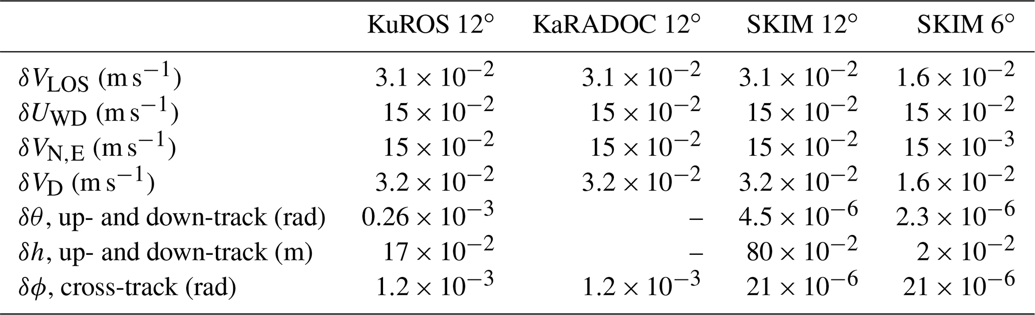
As an illustration, Table 2 summarizes the requirements that have to be met to keep the standard deviation of each of the seven terms below 0.15 m s−1, ensuring a 0.4 m s−1 standard deviation for UCD. The requirement for θ is translated to the corresponding altitude-tracking accuracy requirement for the KuROS and SKIM configurations. The requirements for linear velocity components are stringent but can be reached using current-day technology. The requirement for altitude accuracy is easily within the specifications of the SKIM nadir altimeter payload but definitely out of reach of KuROS. The KuROS data could, however, be analyzed in the cross-track-looking configurations for which this requirement does not apply. The requirement for azimuthal pointing accuracy is by far the most stringent. In the airborne case, it is met for the antenna boresight by the plane IMU (inertial measurement unit), allowing a straightforward analysis of the KaRADOC data. In the KuROS case, however, it is exceeded by a factor of 10 by the mispointing induced by the azimuthal gradients of sea surface, which required the development of a specific data correction procedure. Finally, in the spaceborne case, it seems only achievable using a combination of high-end inertial measurements and data-driven analysis techniques.
This section provides a general overview of the campaign. The location, timing and overall organization are described in Sect. 3.1, the environmental conditions encountered during the campaign are described in Sect. 3.2, and the two main instruments, the KuROS and KaRADOC airborne radars, are described in Sect. 3.3 and 3.4, respectively.
3.1 Campaign organization
The Drift4SKIM experiment differs from previous airborne Doppler radar campaigns (Martin et al., 2016; Rodríguez et al., 2018) in two important respects: in order to observe the effect of wave development on the geophysical Doppler velocity UGD, it was performed in a midlatitude, eastern basin oceanic environment open to offshore swells. Also, given the campaign objectives of demonstrating the sensitivity of airborne radar Doppler measurements to the geophysical contributions of currents and waves, it comprised an extensive in situ component designed to have commonly accepted reference measurements for these parameters.
Fieldwork was performed in two areas (denoted by square boxes in Fig. 6) named the “offshore” area, centered on the Trèfle buoy (see below), and the “Keller Race” area to the north of the island of Ushant. Both locations are in the range of coverage of a two-site WERA (Gurgel et al., 1999) high-frequency radar system, operated by Service Hydrographique et Oceanographique de la Marine (Shom) and already used for several studies, in particular related to wave–current interactions (Ardhuin et al., 2009, 2012; Guimaraes et al., 2018).
Keller Race is an area with very strong horizontal gradients of the current (Sentchev et al., 2013). Although it is easy to show a strong effect of the current on the measured DFS, the spatial variability of the sea state is difficult to measure in situ, introducing uncertainties when combining UCD+UWD in a forward model or using UWD estimates when retrieving UCD from the measured UGD. The offshore area, on the other hand, was chosen for its spatial uniformity, being located far enough from the islands and with a near-uniform depth of 110 m. Only airborne data acquired over the offshore area are presented in this paper.
The week around spring tides in November 2018 was selected in order to allow for a wide range of current speeds (Fig. 7a).
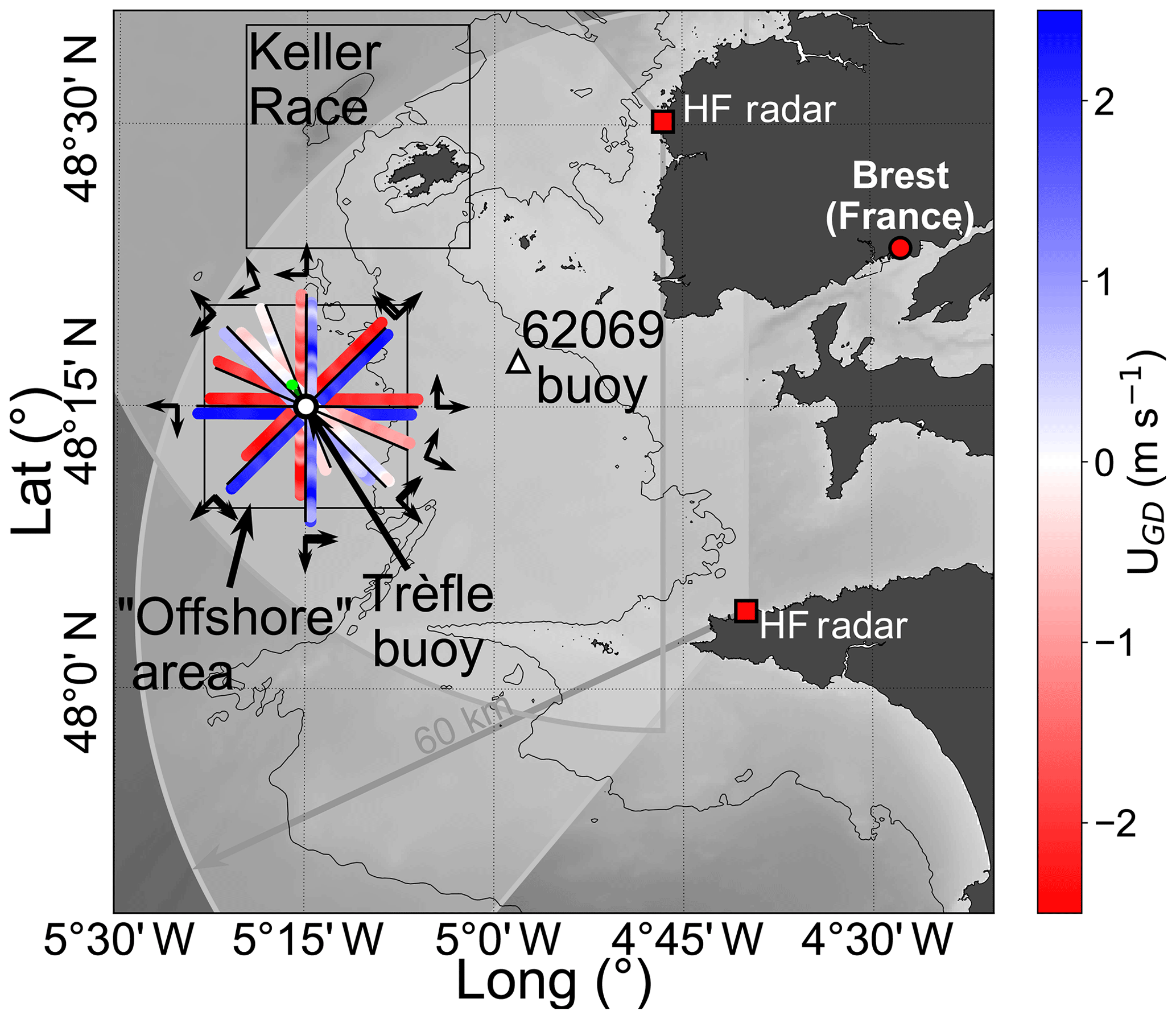
Figure 6Location of the measurement campaign and in situ assets, including a map of the KaRADOC measurements of the geophysical Doppler velocity UGD acquired on 22 November 2018.
The KuROS and KaRADOC radars were installed on an ATR-42 plane operated by the French institutional scientific flight facility, SAFIRE, which is equipped with an AIRINS™ GNSS-FOG INS providing position, pitch, roll and heading information with stated tolerances of a few centimeters, 0.005, 0.005 and 0.01∘, respectively.
Ground truth measurements comprised two permanent operational systems: the HF radar system mentioned previously, with an expected depth of measurement around 1 m (Stewart and Joy, 1974), and the Pierres Noires (WMO no. 62069) wave-measuring buoy. Dedicated instrumentation was also deployed for the campaign.
-
The Trèfle buoy was moored at 5∘15′ W, 48∘15′ N at the center of the offshore area. This buoy monitored the surface current (Sutherland et al., 2016) and provided directional wave spectra (Fig. 8).
-
Several types of drifting buoys, including CARTHE drifters (Novelli et al., 2017) drogued around 40 cm, SVP drifters (Niiler and Paduan, 1995) drogued at 15 m and Spotter wave-measuring buoys (Raghukumar et al., 2019), were deployed in the measurement areas.
-
The R/V Thalia worked in the offshore area, providing continuous underway measurements of meteorological parameters using a Météo-France BATOS operational system comprising a Vaisala WXT series sonic anemometer located approximately 10 m above the sea surface. The ship also carried a SBE21 thermosalinograph.
In the summer, the so-called Ushant tidal front has a strong influence on the surface currents, as well as hydrographic (Le Boyer et al., 2009) and atmospheric (Redelsperger et al., 2019) conditions in the offshore area. This seasonal feature typically disappears in October, and conductivity–temperature–depth (CTD) casts were performed from R/V Thalia to confirm that it had indeed vanished when the campaign took place. The water column was found to be very well mixed, with surface-to-bottom potential density anomalies being smaller than 0.002 kg m−3. The spatial homogeneity was also checked using the ship thermosalinograph and an infrared camera mounted on a Piper PA-23 plane, which surveyed the offshore area in a “lawn-mowing” pattern, flying under the clouds at an altitude of 500 to 1000 m. While small-scale surface features were observed on calm days, it is clear that no density-associated mesoscale structures were present.
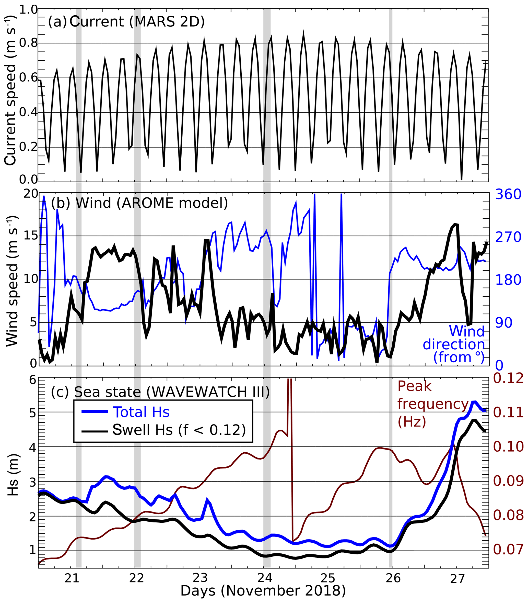
Figure 7Time series at the location of the Trèfle buoy (5∘15′ W, 48∘15′ N) in the offshore zone of (a) ocean surface current speed from the MARS2D numerical model run at LOPS (Lazure and Dumas, 2008). (b) Wind speed (black) and direction (blue) from the AROME regional operational model run by Météo-France. (c) Total (blue) and swell (black) significant wave height and wave peak frequency (red) from the WAVEWATCH III numerical wave model run at LOPS (Roland and Ardhuin, 2014). The four time periods shaded in gray correspond to the times of fixed-antenna KuROS measurements. The corresponding observed environmental parameters are detailed in Table 3.
The airborne radar measurements geometry over the offshore area consisted of relatively long (12 km) and straight tracks with different aircraft headings, forming a star pattern, as for the 22 November 2018 flight shown in Fig. 6. Tracks were flown every 12, 22.5 or 45∘ in azimuth, depending on flight duration constraints. The KaRADOC antenna was fixed relative to the aircraft and looking to port, while the KuROS antenna could either be fixed in the up-track or port cross-track directions, or it could rotate in the clockwise sense relative to the flight track. The KuROS Doppler data presented in this paper were acquired in the port-looking configuration.

Figure 8Directional wave spectra E(fr,θ), as functions of the relative wave frequency fr and incoming wave azimuth θ, estimated from the motions of the Trèfle buoy on 22 November at 13:00 UTC and Spotter buoy number 10 on 24 November at 12:00 UTC. The measured directional moments were transformed with the maximum entropy method (Lygre and Krogstad, 1986) and Doppler-shifted with for the moored Trèfle buoy. The red and blue arrows represent the AROME wind and MARS2D surface current vectors directions, respectively.
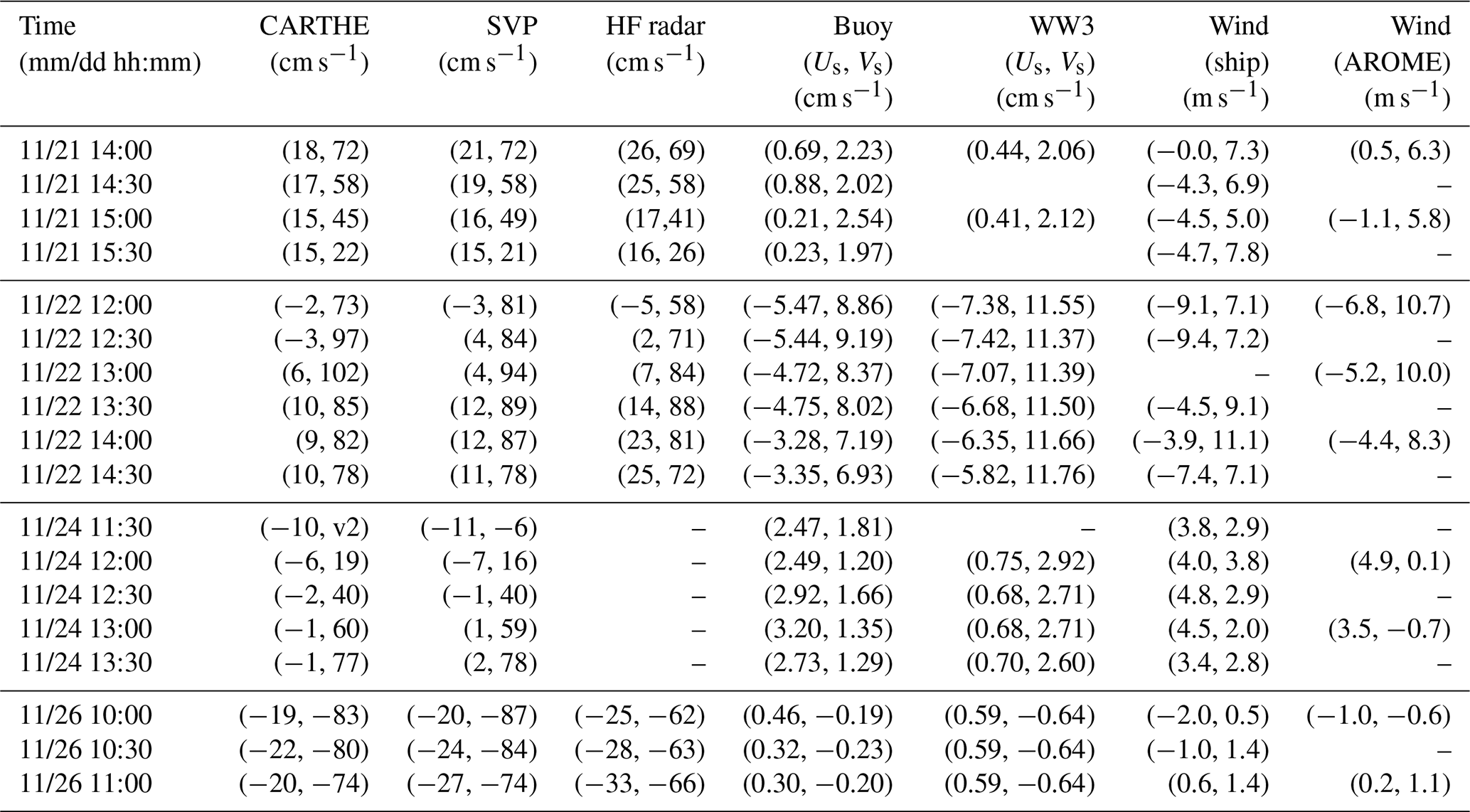
Table 3Surface current velocity, Stokes drift and wind speed measured or estimated near position 48∘15′ N, 5∘15′ W. For each table entry, the parenthesized pair contains the (eastward, northward) components of the vector (cm s−1) for current or Stokes drift estimates and (m s−1) for wind speed estimates. Please note that the Stokes drift is only integrated up to 0.5 Hz. Stokes drift buoy data correspond to the Trèfle buoy for 22 November and Spotter buoy number 10 for 24 November.
3.2 Geophysical conditions
A wide range of geophysical conditions were encountered during the 1-week-long campaign. Four flights were performed over the offshore area on 21 November from 13:50 to 15:50 UTC, on 22 November from 12:15 to 15:00 UTC, on 24 November from 11:20 to 13:20 UTC, and finally on 26 November from 09:40 to 11:00 UTC. In this paper, we focus on data acquired on 22 and 24 November as the geophysical conditions were interesting and complementary (see below), and data were acquired with the largest azimuth diversity on these two days.
The 22 November flight took place at the end of a steady southeasterly wind episode (13 m s−1 from 140∘). The 24 November flight, in contrast, took place during a steady weak southwesterly wind period (5 m s−1 from 225∘) (Fig. 7b).
The wave height during the campaign was dominated by the presence of two swell systems from North Atlantic remote storms. The swell height decreased from 2.5 m on 21 November to 0.9 m on 24 November, with a peak frequency increasing from 0.07 to 0.1 Hz and a mean direction gradually veering from northwest to west. This swell has a small contribution to the Stokes drift of the order of 10 % of the wind-sea contribution on 22 November.
The main environmental conditions at the time of these star-pattern flights are summarized in Table 3.
3.3 KuROS instrument
KuROS is a Ku-band (13.5 GHz) pulse-pair Doppler radar with a dual antennae system and azimuthal scanning possibility, which was developed in the framework of the CFOSAT prelaunch studies. Of the two antennas, the low-incidence (LI) antenna is nominally centered on a 14∘ incidence angle, while the medium-incidence (MI) antenna is nominally centered on a 40∘ incidence angle. Only the LI antenna, which was the more relevant for SKIM, was used during the campaign. This antenna uses a horizontal transmit–receive polarization (HH) polarization. A comprehensive description of the system can be found in Caudal et al. (2014). A new antenna was used for the Drift4SKIM campaign, with characteristics given in Table 1.
The radar transmits a frequency-modulated pulse (chirp) with a 100 MHz bandwidth, achieving a 1.5 m range resolution and an effective ground-projected resolution of approximately 7 m (at 12∘). The one-way 3 dB footprint in azimuth is 580 m wide at 12∘ and 3000 m of flight altitude. The pulse repetition frequency (PRF = 1 ∕ PRI) depends on the altitude and is 23 kHz when the aircraft flies at 3000 m. The ambiguity of the Doppler velocity measurement (see Sect. A1.4 in the Appendix) is about 126 m s−1, which is much larger than expected from the measurements (below aircraft speed of 120 m s−1). In order to reduce the thermal noise contribution, the range-resolved pulse-pair signal is coherently averaged in the instrument over 1 ms, corresponding to 22 pulse pairs per instrument sample. For the purpose of this article, this was further coherently averaged per blocks of 15 samples.
As discussed in Appendix A, accuracy requirements for observation geometry are much less stringent for cross-track than for up-track and down-track Doppler velocity observations. The Doppler velocity data discussed in this article were all collected with the KuROS antenna in the port-looking orientation. This configuration also ensures an overlap with the KaRADOC footprint.
3.4 KaRADOC instrument
The Ka-band RADar for Ocean Current (KaRADOC) airborne radar sensor was developed for the Drift4SKIM campaign. KaRADOC is derived from the Still WAter Low Incidence Scattering (SWALIS) instrument, developed for the measurement of the NRCS of inland water surfaces in the Ka band. Further details on the system are given in Appendix C.
KaRADOC was mounted under the ATR-42 aircraft in a port-looking configuration. The two-way 3 dB footprint from 3000 m of altitude over a flat sea surface is an ellipse with diameters 45 and 60 m in the cross-track and along-track directions, respectively. The antenna is of the slotted-waveguide type and allows steering of the beam in elevation (incidence angle) by varying the working frequency. Data were acquired at different incidence angles from 6 to 14∘, corresponding to a range of frequencies from 32.5 to 38.2 GHz. This article focuses on the observations collected at at 33.7 GHz.
KaRADOC does not implement a range-resolution scheme: the transmitted pulses last several microseconds, and the whole FOV is illuminated simultaneously. The demodulated return signal is sampled at 15 MHz and archived. It is essentially constant while the electromagnetic wave is actually interacting with the sea surface. The useful signal segment is selected and its average is computed in order to reduce the thermal noise contribution, yielding one complex amplitude for each pulse. Several hundred pulses are sent at 4 kHz PRF for each burst of measurements, with a burst repetition frequency of the order of 5 to 10 Hz, depending on the number of incidence angles in the scanning sequence. These parameters were varied during the acquisitions. Though they have a strong impact on NRCS and DFS estimate quality, we have found the low-pass-filtered DFS signal to be robust.
The pulse-pair complex signal is averaged for each burst in order to reduce the effect of coherent speckle. One complex pulse-pair sample is thus obtained per burst. Even at the lowest burst repeat frequency of 5 Hz, the plane moves by less than a third of the FOV along-track extension between bursts.
The impact of the acquisition parameters on the KaRADOC measurement normalization is not yet fully understood, and the NRCS measurements could not be exploited in the scope of this study. The noise-filtered DFS measurements are, however, not affected by these normalization changes and are valid.
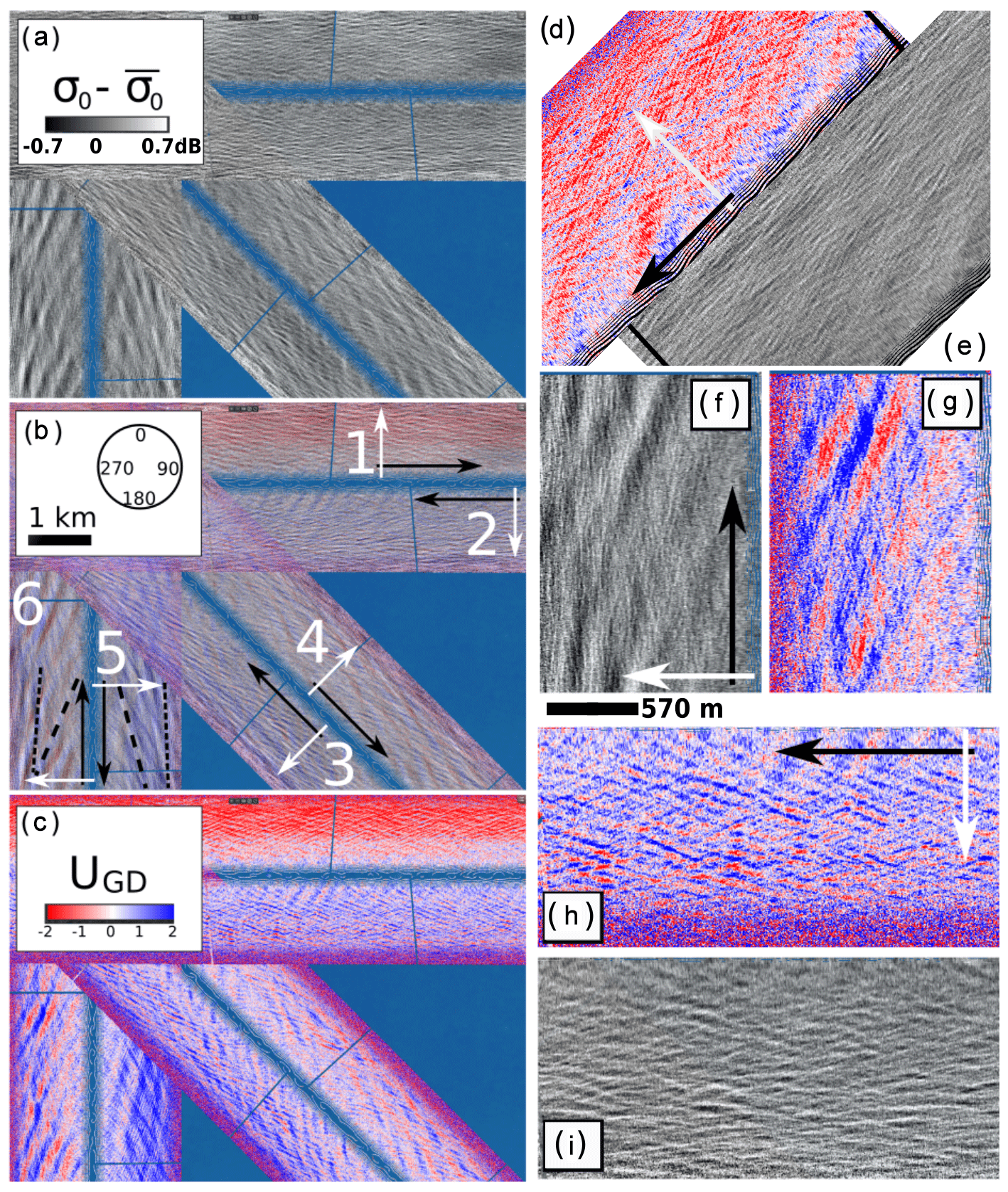
Figure 9(a, c) Mosaics of KuROS backscattering intensity and Doppler velocity data acquired on 22 November with fixed port-looking antenna. (b) Overlay of the Doppler velocity and backscattering intensity. Flight tracks are numbered 1 to 6; black arrows indicate the flight direction, and white arrows point in the radar look direction. The long dashed lines represent the apparent direction of swell crests. Panels (d)–(i) show close-up views of selected tracks from (a) and (c). The tracks shown in (d) and (e) are out of the frame of (a) and (c). Panels (f)–(i) show close-ups of flight tracks 6 and 2. The 570 m scale bar applies to (f)–(i) and corresponds to the along-track 3 dB width of the radar beam at a 12∘ incidence angle, i.e., near the middle of the swath. The mean trend of σ0 as a function of θ has been removed from the σ0 data.
4.1 KuROS NRCS–DFS imagery
The KuROS NRCS–DFS imagery reveals a host of interesting features, modulations and dependencies. An in-depth analysis of all these processes is clearly out of the scope of this paper and will be the subject of forthcoming contributions from the Drift4SKIM team. This section thus only provides a cursory description of a few segments of σ0 and DV data collected on 22 November 2018 when the wind speed was approximately 11 m s−1, which are displayed in Fig. 9.
A first remark is that the NRCS is smooth, with a typical modulation depth of 1 dB after removing its mean trend as a function of incidence angle (Fig. 9a). This smoothness is in part due to the large footprint, but it also shows that the radiometric quality of the data and the coherent averaging performed are sufficient to control the thermal noise. Speckle noise is, however, still present, with different statistics depending on the radar look direction and the variable considered (not shown). The cross-track observation geometry leads to the best speckle noise reduction for the NRCS but to the worst-case speckle noise statistics for the DV.
The KuROS data clearly show a modulation in both NRCS and UGD associated with the northwesterly swell observed by the Trèfle buoy with a peak frequency of 0.07 Hz, corresponding to a wavelength L=320 m (Fig. 8). This is particularly visible on the north–south-oriented flight tracks numbered 5 and 6 in Fig. 9b (see also Fig. 9f–g for a zoom-in on track 6). The apparent swell crest direction (dashed lines in Fig. 9b) differs from the true direction due to the scanning distortion effect (Walsh et al., 1989; Sutherland et al., 2018), as the swell propagates during the measurements at a phase speed of 22 m s−1, while the aircraft moves at 120 m s−1.
The shorter waves measured by the Trèfle buoy (Fig. 8) occupy a wide range of directions from a narrow wind-sea peak from the south at 0.16 Hz (L=60 m) to a broad directional distribution at 0.22 Hz (L=30 m), with a mean direction of 130∘ and a half-width (spread) of 45∘, hence covering directions from 85 to 175∘. These shorter components are present in the data from flight tracks 5 and 6 in the form of very narrow stripes with orientations shown by short dashed lines in Fig. 9b (see also Fig. 9f–g for a zoom-in on track 6). The “long-crested” appearance of the short waves in (d) and (e) is an artifact due to the wavefront-matching observation geometry (Jackson et al., 1985), with all other directions averaged out by the large azimuth width of the radar beam. If purely geophysical, the phase relationship between the DV and NRCS modulations is expected to give the wave propagation direction. For flight track 6 in (f) and (g), the long swell propagates towards the radar, and the brighter slopes (white) correspond to eastward velocities toward the radar (blue). This will be discussed in further detail below. Finally, (h) and (i) exhibit chevron patterns with crests facing both northeast and northwest. Whereas the waves from the southwest are expected to be much longer than those from the southeast, this is not apparent in the KuROS data.
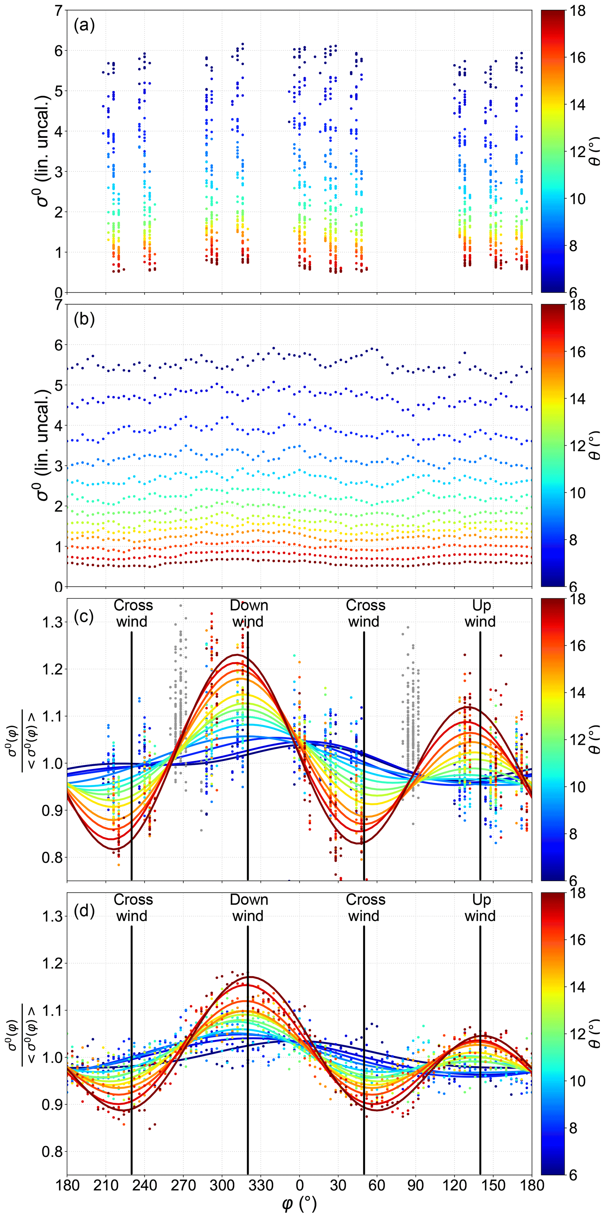
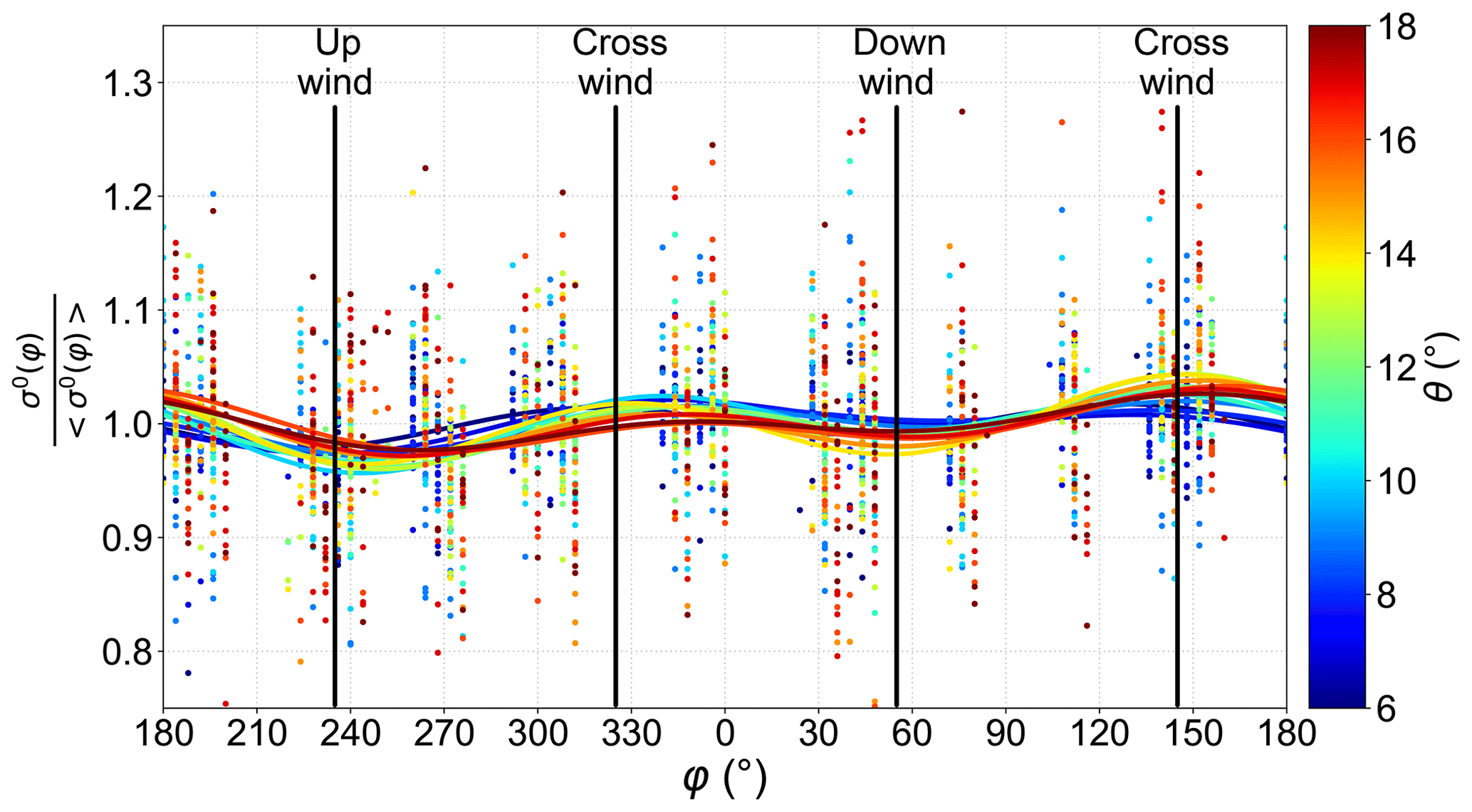
Figure 10(a, b) Variations as a function of azimuth φ of σ0 for an incidence angle θ of 6 to 18∘ on 22 November for the port-looking (12:13–13:38 UTC) and rotating-antenna (13:41–13:58 UTC) flights, respectively. (c, d) Variations of σ0 normalized by its azimuthal average for the fixed- and rotating-antenna data, respectively.
4.2 Ku-band NRCS
In this section we discuss the dependence of the Ku-band NRCS as a function of azimuth and incidence angle for the 22 and 24 November cases. The fixed-antenna and rotating-antenna data are presented. In order to reduce the dispersion introduced by the short-scale modulating processes discussed above, the data were averaged per 1∘ incidence angle and azimuth bins. As mentioned before, full tracks are straight and relatively long (12 km), and they view a mainly homogeneous ocean region. For the fixed-antenna observations, azimuthal diversity is obtained by performing tracks in different flight directions, forming a “star” pattern.
The variations of the Ku-band σ0 are shown for 22 November in Fig. 10. These measurements show the expected modulation of 0.8 to 0.9 dB with azimuth, with a downwind–crosswind contrast that increases with the incidence angle. This contrast is larger for the higher winds on 22 November. The upwind–downwind asymmetry is expected from the behavior of the surface slope probability density function (Chapron et al., 2002; Walsh et al., 2008; Munk, 2008). The exception are the σ0 values for the flight tracks with a fixed antenna around the azimuths 90 and 270 (Fig. 10a), which have anomalous normalized values between 1 and 1.3 instead of expected values much closer to 1. We have no explanation for this anomaly, which is genuine. No such anomaly was found for the rotating-antenna data collected later on the same day (Fig. 10b).
Discarding these azimuth ranges (shaded in gray in Fig. 10c), the data could be well fitted with a functional form . As explained in Sect. 2.1, measuring this azimuthal variation is critical for the interpretation of the mean Doppler velocity due to the spurious azimuth gradient contribution. As expected, the fitted directions φσ,1 and φσ,2 are very close to the wind direction, except for the lowest incidence angles for which the contrast is less than 0.05 dB.
On 24 November, the σ0 azimuthal contrast was much weaker (Fig. 11) due to the much lower wind speed and was actually not aligned with the wind direction when the measurements were performed.
4.3 Mean Doppler velocity from KaRADOC
We now quantitatively discuss the measured Doppler velocity signal in order to assess the agreement of our theory of the wave-induced contribution UWD with the measurements. This section is focused on the KaRADOC data, which are easier to interpret than the KuROS data due to the narrower radar beam of the instrument.
We present in Fig. 6 the low-pass-filtered UGD estimates retrieved from the 12∘ incidence angle KaRADOC data collected on 22 November between 12:13 and 12:59 UTC.
This representation is misleading, as much of the observed variability is in fact due to the effect of the flight track orientation. For instance, the largest contrast can be observed between the northeastward- and southwestward-directed flight tracks, even though to a first approximation a mere change in observation direction has occurred.
Another representation of the same data is proposed in Fig. 12. In this figure the UGD data are represented as blue lines shifted to the right of the plane ground track (in black) by an amount proportional to the instantaneous low-pass-filtered UGD value. This representation removes the trivial effect of observation direction changes and allows subtler effects to be better appreciated. For instance, noise-free observations of a constant vector UGD would appear as straight lines parallel to the flight tracks, all crossing at the tip of the vector. Deviations from this behavior, such as can be observed in Fig. 12, are indicative of measurement noise, geophysical variability or geophysical phenomena not accounted for by our theory.
For 22 November, 16 flight tracks are available collected from 12:13 to 12:59 UTC, and for 24 November 17 tracks were collected from 11:27 to 13:13 UTC.
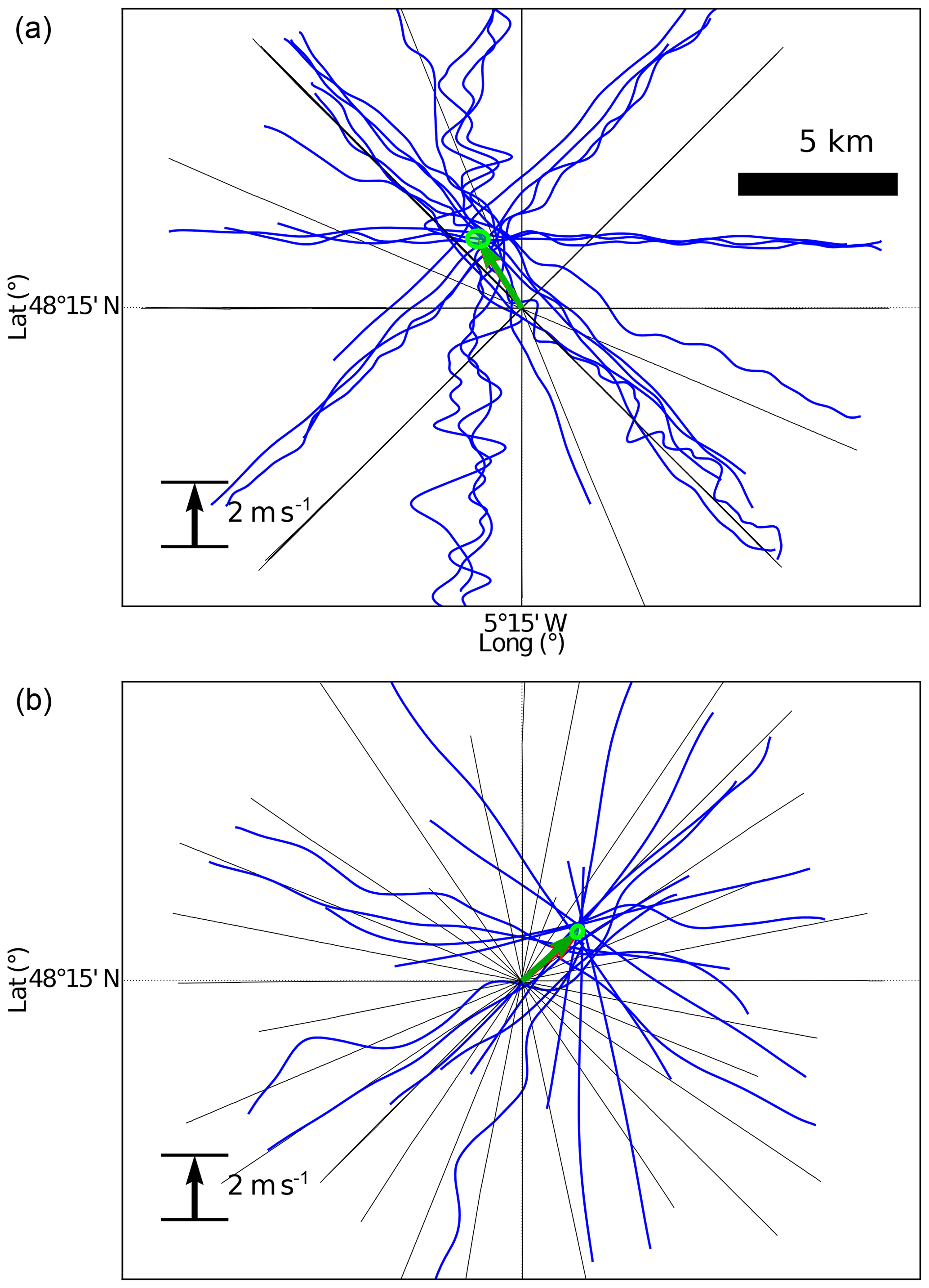
Figure 12Plots of the Ka-band Doppler velocity signal on (a) 22 and (b) 24 November 2018. The flight tracks are marked as thin black lines. For each flight track, a thick blue line shifted to the right of the flight path by an amount proportional to the instantaneous low-pass-filtered Doppler velocity represents the projection of the UGD vector along the instrument line of sight. At the beginning of each track data were discarded until the plane stabilized. The green arrow represents the maximum likelihood estimate of the UGD vector using the whole data set. The (almost indistinguishable) red arrow shows the result of the least-squares sinusoidal fits shown in Fig. 13a and b. The 1 standard deviation error ellipse on the maximum likelihood estimate is represented in green.
Overall, the assumption of a constant vector is good to within 0.3 m s−1. It is particularly striking that the three horizontal lines in Fig. 12a are almost perfectly aligned, corresponding to two flight tracks looking into azimuth 0∘ and one flight into azimuth 180∘. On 22 November, the largest dispersion is for the 315 and 135∘ azimuths for which a total of four tracks are available with very different values that are, however, consistent along each track.
Using the average values from the different tracks, we compare the measured Doppler velocity to the forward model given by Eq. (1), with UWD estimated from the in situ wave buoy data using the tools discussed in Sect. 2.2. The method combines the buoy spectrum up to 0.35 Hz and adds a high-frequency tail based on the Elfouhaily (1997) spectrum, then computes numerically the integrals of Eqs. (8) and (9) to obtain the DFS estimate. The TSCV contribution, UCD, is taken to be the drift velocity of the nearest CARTHE drifter, which is uniform to within 3 cm s−1 in the offshore area (interactive animations of all deployments and trajectories can be found at https://odl.bzh/eVRHv1TE, last access: 25 October 2020).
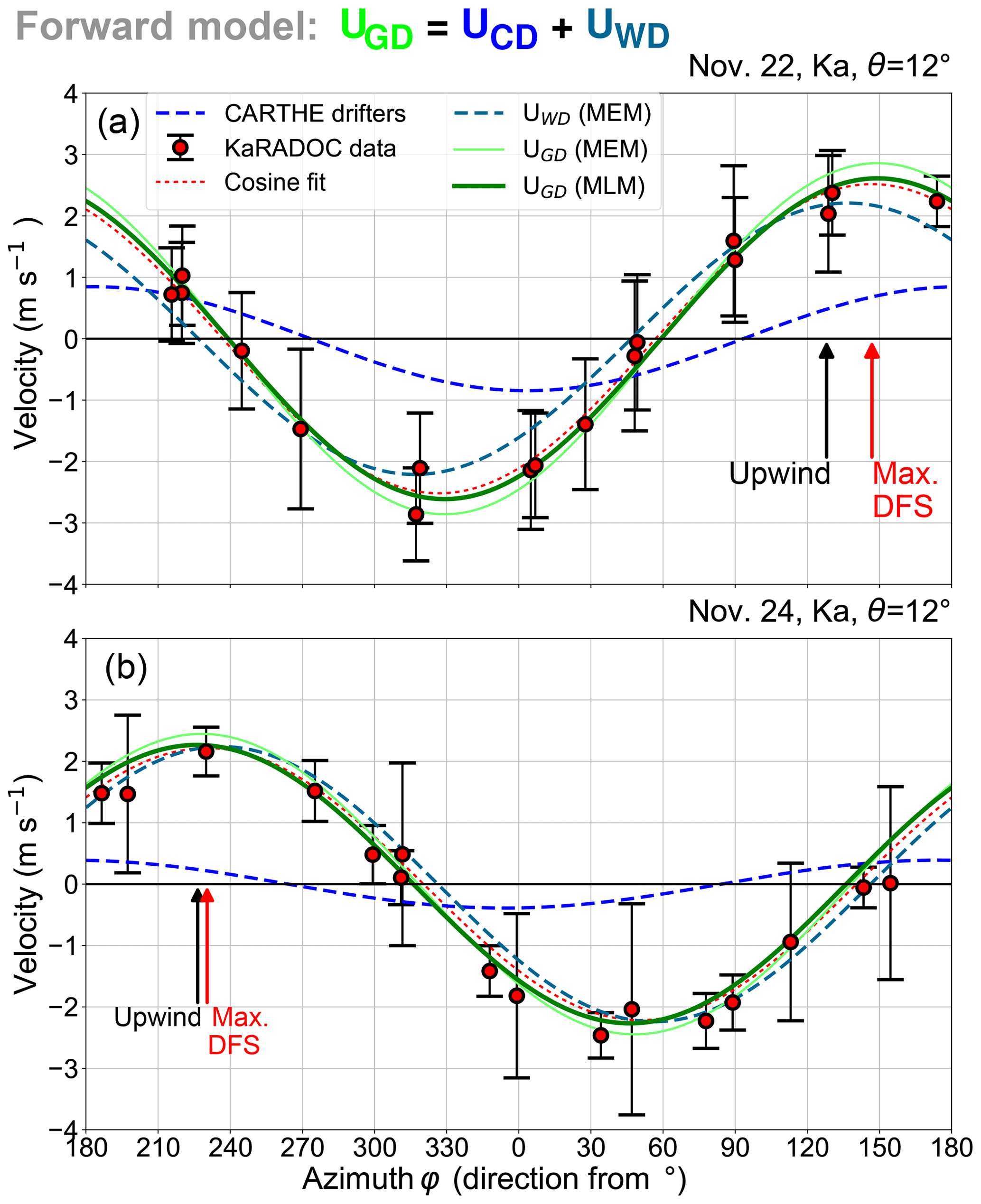
Figure 13KaRADOC Doppler velocity (red circles) for the star-pattern flights on (a) 22 and (b) 24 November. Cosine function fits to the data (red lines). Modeled geophysical Doppler velocity UGD using the MEM (MLM) estimate of the directional wave spectrum (green and darker green). The modeled UGD is the sum of the CARTHE drifter velocity UCD (blue) and the wave Doppler velocity estimated from the measured spectra, UWD (midnight blue dashes).
Figure 13 shows the measured mean Doppler velocity and standard deviation for each track (the standard deviation is representative of the order of magnitude of the short-scale modulations due to waves, not of the error bar for the mean DV). On 22 November (Fig. 13a), the current vector accounts for less than half of the observed magnitude of UGD, and it is interesting that the maximum Doppler velocity is from azimuth 147∘, between the wind direction (128∘) and the up-current direction (183∘). The directions of the modeled and measured UGD are within 5∘ of each other.
Compared to the relatively high wind condition on 22 November, it is interesting to discuss the results for 24 November (Fig. 13b), with a wind speed of 5.5 m s−1 instead of 11 m s−1. The amplitude of the Doppler velocity is not much reduced, in spite of more than halved current and Stokes drift. This is consistent with the expected near-constant value C0 of the wave Doppler velocity magnitude, and this is the main result of the present paper.

Figure 14TSCV retrieval UCD (in blue) obtained by subtracting the UWD from the MLM-processed Trèfle buoy data (in midnight blue) from the UGD vector determined from the KaRADOC measurements (in red) compared to field measurements by HF radar, CARTHE and SVP drifters (shades of gray) on (a) 22 and (b) 24 November.
The process leading to the estimation of the constant C0 is, however, dependent on a number of assumptions: the directional wave spectrum must be evaluated from the buoy data, then matched to a parametric spectral shape before the necessary numerical integrations can be performed. The (Elfouhaily et al., 1997) spectral shape we have used depends on the wind speed and direction, but also on a wave age parameter, Ω, equal to 0.84 for equilibrium seas.
Table 4 summarizes a subset of the extensive tests we have performed to check the sensitivities of this process. It is clear from this table that drastically changing the wind speed, as occurred between the two days, affects the magnitude of the computed UWD more at the Ku band than the Ka band, but not in a catastrophic way, and that the wave age parameter Ω can also be varied over its meaningful range quite freely. We have also checked that the transition frequency at which the spectral tail is matched to the observational data is not a very sensitive parameter, provided it is taken low enough for the buoy data to be of good quality where they are kept.
Extracting directional wave spectra from buoy data, however, is a quite an intricate and subjective step. Several methods have been developed over the years to this end, each with pros and cons (see Benoit et al., 1997, for a review). Two of the best-established methods are the maximum entropy method (MEM) and the maximum likelihood method (MLM). The MEM is a parametric method which assumes a specific form of the directional spreading function. In each frequency band, the parameters of the spreading function are chosen such that the first moments of the azimuthal Fourier spectrum match the buoy-derived ones. The MLM is a nonparametric method akin to the Capon beamformer. In terms of directional moments measured by buoys, the MEM estimates provide spectra that exactly fit the measured moments, while the MLM produces spectra that have directional spreads larger than those obtained directly from the measured moments. However, it is not clear how they compare on other properties of the spectrum that may be relevant to the mean slope velocity. Comparing results obtained with these two methods was thus a convenient way to test the sensitivity of UWD to the sea state directional spread.
Table 4Modeled wave Doppler velocity amplitude MWD and direction φWD at the Ku and Ka band with directional wave spectra produced using the maximum entropy or maximum likelihood methods and varying the wave age parameter Ω of the Elfouhaily (1997) high-frequency spectral tail. In all cases the transition frequency between the wave data and the high-frequency spectrum is ft=0.35 Hz. All values are estimated for .
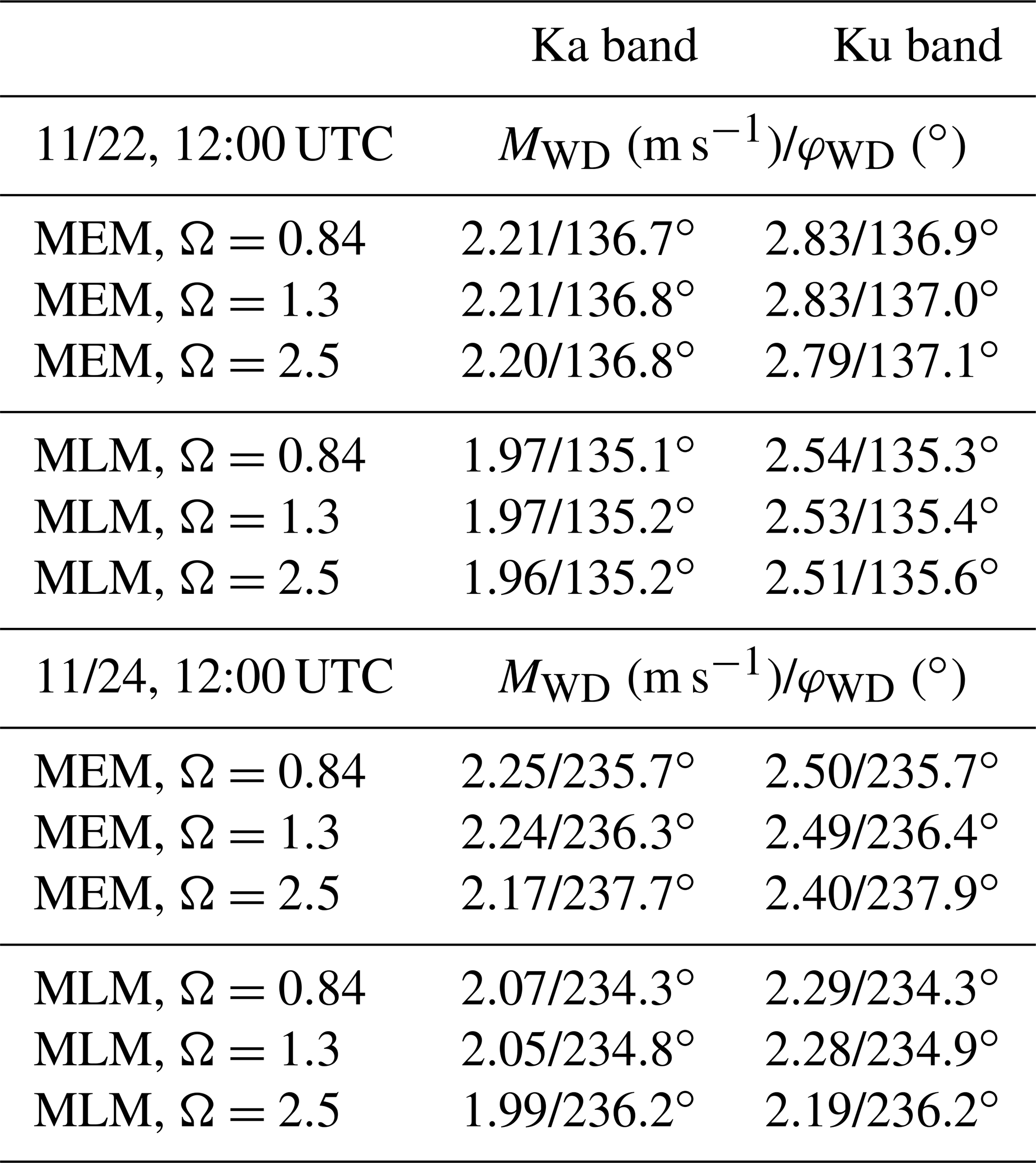
As Table 4 shows, using one technique or the other to estimate the resolved part of the wave directional spectrum does induce significant differences in the simulated UWD values, showing that the azimuthal width of the spectrum, which is currently not very well constrained observationally, is a sensitive factor. The values obtained using the broader MLM spectrum are consistently smaller than those obtained using the MEM spectrum. A broader azimuthal distribution only redistributes the weight between the different Mss components but reduces the contributions composing the msv0 vector.
The results obtained using both methods are shown in Fig. 13 as light green and dark green lines. It appears that the MLM processing of the buoy data gives the best fit to the radar UGD, showing that the directional spread of the sea state should not be taken too low. The possibility that the directional distribution of the Elfouhaily (1997) spectrum could be slightly too narrow for intermediate wavelengths of 2–10 m was, for instance, discussed in specific cases by Peureux et al. (2018). It is, however, not yet clear if it is specific to the very young wind seas they observed, although it could also explain some properties of L-band backscatter (Yueh et al., 2013). The MLM was used to process the Trèfle data in the rest of this study.
Conversely, Fig. 14 illustrates the use of the DV data for the retrieval of the surface current vector by subtraction of UWD from the fitted UGD. The norm of the difference between the in situ measured and remotely sensed UCD vectors is less than 20 cm s−1 on both days, which is significant but quite satisfying at such an early stage of the technique, especially taking into account the fact that geophysical variability due to time variations of wind and tidal current occurred over the several hours of the flight.
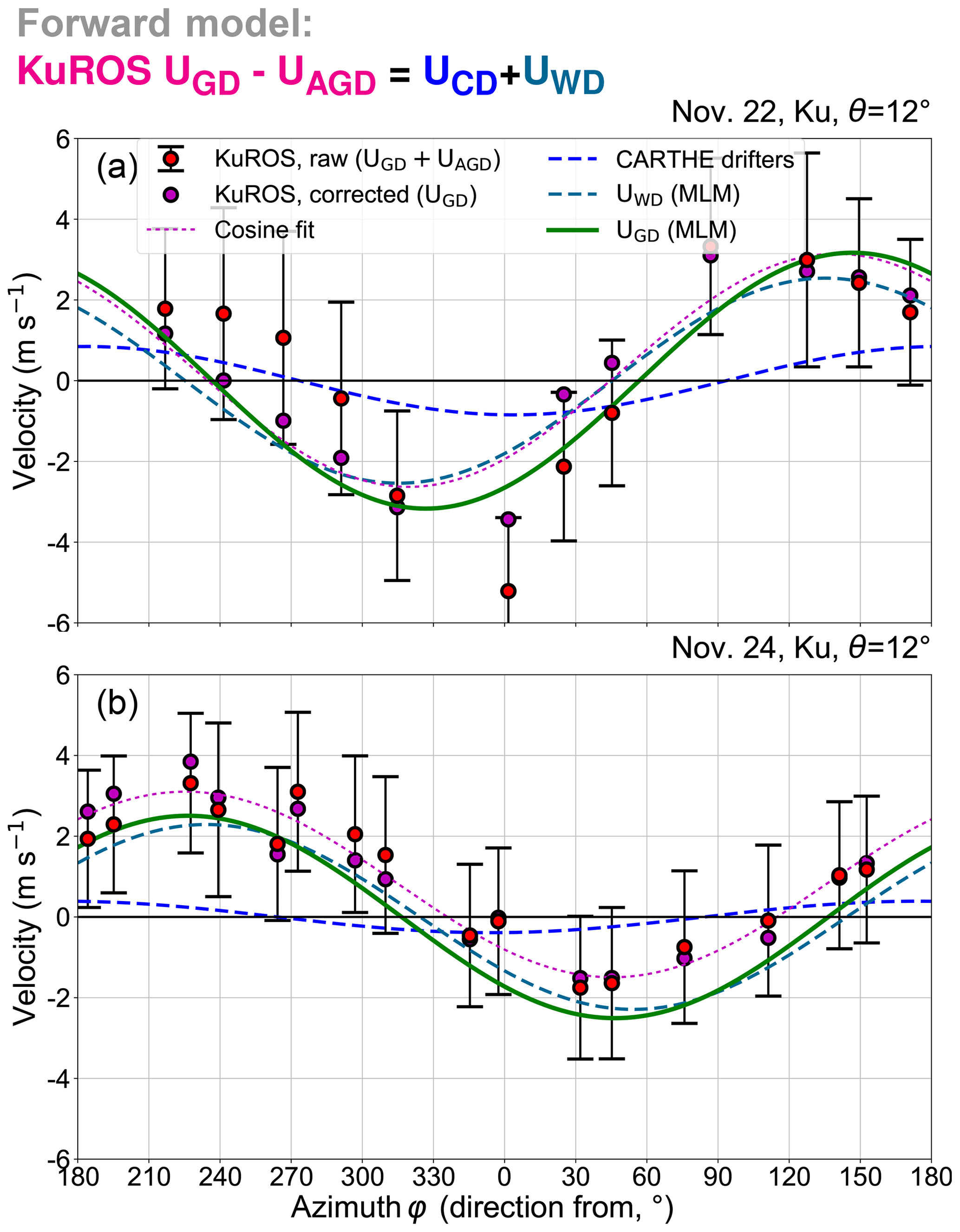
Figure 15Ku-band Doppler measurements performed on (a) 22 November and (b) 24 November with the KuROS radar in the port-looking antenna configuration at a incidence angle. The graphical conventions are identical for the two plots. The red dots and error bars represent the average and ±1 standard deviation interval of the platform-motion-corrected DV measurements along the different tracks. The magenta dots mark the mean values after correction of the UAGD contribution. The magenta dotted line is the cosine fit to the corrected data. The blue and midnight blue lines respectively represent the projection along the line-of-sight azimuth of the CARTHE current measurements and the UWD vector computed from the MLM-processed Trèfle buoy data. The green line represents the sum of these two contributions and should agree with the magenta dotted line.
4.4 Mean Doppler velocity from KuROS
Due to the much broader radiation diagram of the KuROS antenna, analyzing the Ku-band data requires significantly more effort, as the UAGD spurious velocity contribution due to the azimuthal variation of σ0 across the FOV discussed in Sect. 2.1 must be compensated for. The DV measurements, corrected for the UNG platform motion contribution but not for the UAGD contribution, are represented in Fig. 15 as red dots, while the green line represents the projection along the line-of-sight azimuth of the sum of the TSCV and the MLM-derived UWD vectors. The difference is clearly very large, reaching 2 m s−1 in places on 22 November, and smaller on 24 November as the azimuthal modulation of the radar NRCS is much weaker.
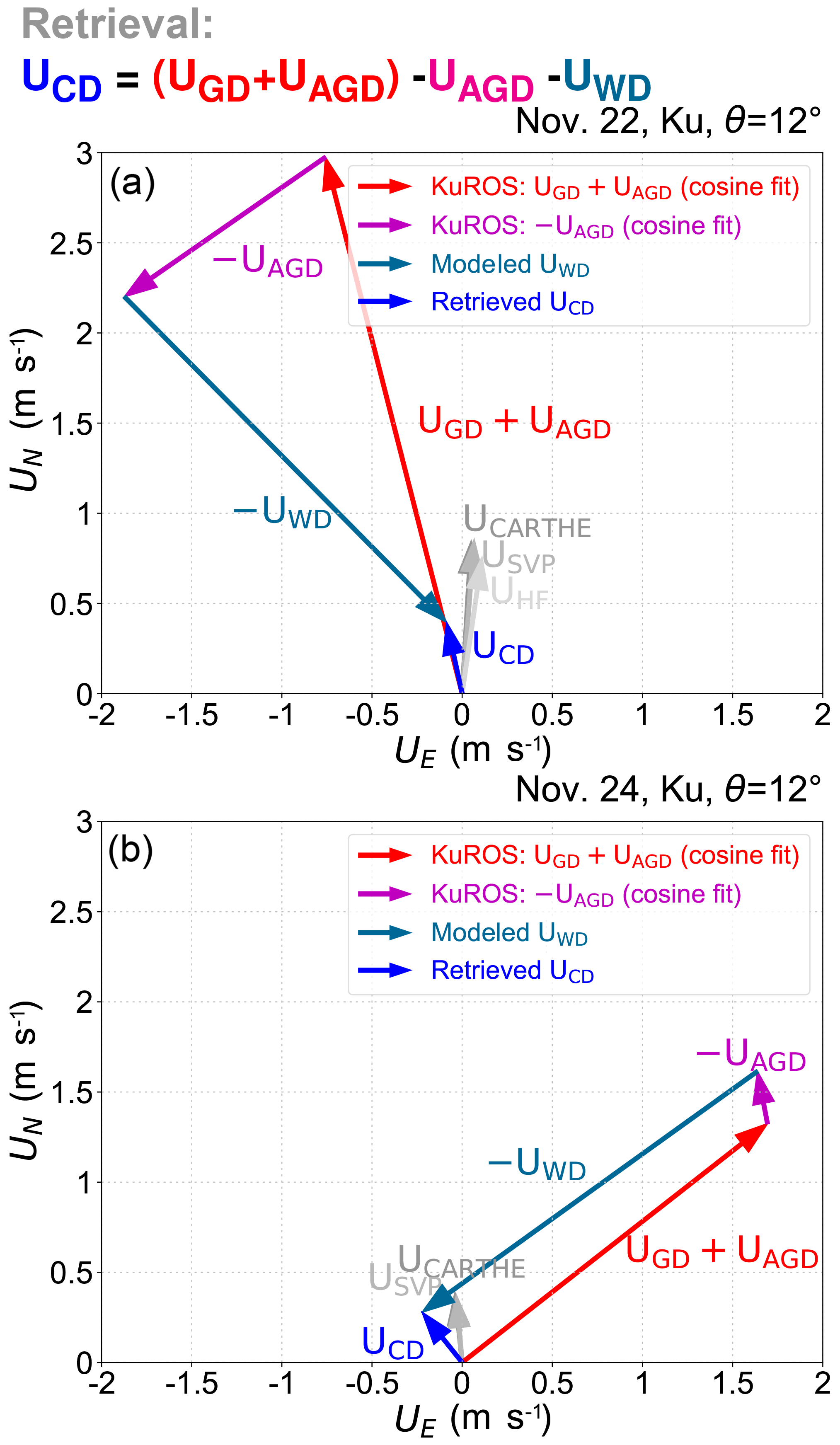
Figure 16Comparison of KuROS-derived Doppler velocity, corrected for the UAGD and UWD wave contributions, with in situ (CARTHE, SVP drifters and HF radar) current measurements on (a) 22 and (b) 24 November.
Introducing the fits to the Ku-band NRCS data discussed in Sect. 4.2 in Eq. (A24) allows one to produce the corrected data represented by the magenta dots, which are in much better agreement with the green line (though a constant offset is apparent in the 24 November data, which is rejected by the cosine-fit procedure). Figure 16 summarizes the UCD retrieval operation in vector form (the magenta arrow represents only the first azimuthal harmonic component of the UAGD correction). The norm of the difference between the in situ (in gray) and remotely sensed (in blue) estimates of the TSCV is of the order of 0.5 m s−1 on 22 November and of the order of 0.2 m s−1 on 24 November. Again, these numbers, though admittedly not small, can be considered encouraging given the number of very large corrections applied to the data and the fact that the instrument had definitely not been designed for this purpose.
4.5 Observed Doppler velocity modulations
The range-resolution scheme implemented in KuROS makes it a very interesting instrument for the analysis of DFS and NRCS modulations. In particular, Caudal et al. (2014), with a different antenna (slightly narrower beam), have attempted to use the cross-spectrum of the DFS and NRCS to resolve the 180∘ ambiguity in the wave propagation direction. In the SKIM context, analyzing the contribution of the resolved scales to the correlation between σ0 and the DFS could permit the development of empirical methods to estimate the unresolved part and provide estimates of UWD.
In practice, with the antenna used for the Drift4SKIM flights, another contribution to the DFS modulations is also caused by the gradients of σ0 and the speed of the aircraft, just like the mean spurious UAGD velocity. Brighter areas in the field of view tend to strongly influence the DFS signal towards positive values if they are located to the front of the aircraft and negative values if they are located aft of the aircraft.
As a test of this, simulations were performed with the Radar Sensing Satellite Simulator (Nouguier, 2019), which are illustrated in Fig. 17. The amplitude of the spurious modulations is enhanced by 70 % when the antenna diagram is made 50 % wider in azimuth. With typical variations of σ0 up to 1 dB over scales of the order of 1 km (e.g., Fig. 9), the variation of σ0 with azimuth φ is roughly proportional to 1∕sin θ, giving a UAGD that does not vary much with θ, of the order of 1.5 m s−1. This spurious velocity is larger than the 0.5 m s−1 significant orbital velocity of the swell. As a result the phase relation between DFS and σ0 can change sign as a function of azimuth due to the combination of two imaging mechanisms with comparable magnitudes and possibly opposite signs.
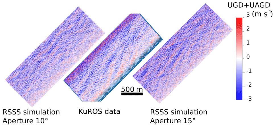
Figure 17Qualitative validation of the R3S simulations of the radar imaging mechanism (Nouguier, 2019). Both the real data and simulation contain the geophysical modulation of velocities associated with surface velocities and slopes in the look direction (part of UGD) as well as aircraft velocities and slopes in the flight direction (part of UAGD). Note that the wave phases in the R3S simulation are random and cannot be expected to match those in the data or between the two simulations.
This effect will be weaker for shorter (wind-sea) components as soon as the wavelength and crest length become much shorter than the KuROS footprint Ly, as given by Eq. (A36): for a given σ0 contrast, the gradient increases linearly as the scale L is reduced, but the UAGD for a given gradient is reduced exponentially in .
The use of two Doppler radars, in the Ka and Ku band with the same pulse-pair technique but antennas with very different radiation diagrams, has provided important insight for the preparation of the SKIM mission.
Regarding radar measurements, the Drift4SKIM campaign clearly demonstrated the feasibility of the TSCV retrieval approach proposed for SKIM (Ardhuin et al., 2018; ESA, 2019) based on the use of the SKIM wave spectrum measurements (here replaced by in situ buoy measurements) to estimate the wave Doppler velocity contribution UWD associated with the wave intrinsic phase speed. Measuring the first directional moments (on which the buoy estimates are based) is sufficient to estimate UWD, and resolving wavelengths of 15 m (a frequency of 0.32 Hz) is sufficient to estimate the full spectral contribution, appending a parametric spectral shape for the unresolved shorter waves. In fact, it is most important to resolve the peak of the wind sea, and a resolved wavelength of 30 m is typically enough for wind speeds higher than 7 m s−1. As this article has shown, however, the angular distribution of the directional spectrum is a sensitive element in both the resolved and parameterized wavelength ranges. Work is still needed to improve the spectral parameterization and to determine whether the accuracy of the sea state restitution algorithms intended for SKIM will be sufficient to solve this issue.
This experiment has also increased confidence in the use of forward models based on the Kirchhoff approximation, such as the R3S of Nouguier (2019), for the study of higher-order effects on the measured DFS. A subject of particular interest is, for instance, the effect of shear in the surface layer on the SKIM DFS, a key to the determination of the effective SKIM measurement depth.
The campaign also stressed the necessity of very good knowledge of the measurement geometry, including the antenna radiation diagram, and the spatial and azimuthal variation of the radar cross section. In this respect, the main characteristics of the instruments used for the present campaign and for the planned SKIM satellite mission are recalled in Table 5, together with the value of the prefactor of the term in Eq. (6) of UAGD (as can be seen in Fig. 10, ∂φlog (σ0) is typically 0.1 rad−1 at a 12∘ incidence angle). As the apparent mispointing due to σ0 gradients in azimuth or space is proportional to the beamwidth squared, the non-geophysical velocities caused by this effect for SKIM, though non negligible, are actually much smaller than for KuROS, even at a 6∘ incidence angle.
Table 5Main differences between the KaRADOC and KuROS airborne radars used in the present article and the SKIM system as presented by the ESA (2019). The factor is the prefactor of in the expression of UAGD.
As discussed in Sect. 2.3, due to the much reduced platform velocity, the pointing requirements for airborne systems are much easier to reach than for satellite systems for which a pointing accuracy of a few microradians cannot be achieved by attitude measurements alone (gyroscopes and star trackers) but must use a separation of the geophysical and non-geophysical patterns in the data (ESA, 2019). This data-driven approach is also used in airborne systems for correcting phase biases in the antenna diagram (Rodríguez et al., 2018).
Finally, as discussed in Sect. 2.3, we recall that the incidence angle is estimated from the range measurements in the cases of KuROS and SKIM and estimated directly from the platform attitude for the pencil-beam case of KaRADOC. In the spaceborne context, the local slope of the ocean has to be taken into account, as it can induce a mispointing of the nadir beam of up to 300 µrad (Sandwell and Smith, 2014) and induce a correction in the elevation angle at the observation point.
Other radar system constraints or optimizations for satellite systems are discussed by Rodriguez (2018) and the ESA (2019, chap. 5), with sampling issues further analyzed by Chelton et al. (2019).
The Drift4SKIM campaign clearly demonstrated that surface geophysical velocities can be measured by microwave Doppler radars implementing the pulse-pair method at the Ka band at a 12∘ incidence angle. The Ku-band measurements, though less easy to interpret due to the large antenna beamwidth of the instrument, also supported this view. The campaign data are consistent with a geophysical model function (GMF) that expresses the geophysical DFS as the sum of the range component of the total surface current velocity and a wave DFS that is a weakly varying function of the sea state of the order of 2.0 m s−1 at the Ka band and 2.4 m s−1 at the Ku band. This wave DFS integrates contributions of all wavenumbers and directions, weighted by the surface slope spectrum. It can be well estimated from the sea surface elevation directional spectrum using the Kirchhoff approximation framework.
The campaign highlighted the importance of very good knowledge of the platform motion and orientation as well as the radar line-of-sight direction vector. The Ku-band NRCS–DFS imagery, though not very successful in that respect, observed a large number of interesting modulation phenomena, which will be analyzed in more detail in forthcoming contributions.
In general, the robustness of the theoretical GMF and its possible empirical adaptation will require the acquisition of more data in a wider range of wind and wave conditions. An in-depth investigation of the angular width of the sea state directional spectrum in the short gravity wave regimes seems of particularly high interest in this respect. Also, obtaining a description of the scale-resolved statistics of sea surface slope skewness would open the path to a Kirchhoff approximation study of the upwind–downwind asymmetry of the radar NRCS and DFS, which is currently lacking.
Finally, the test of near-nadir satellite measurements is limited by the very different viewing geometry due to the difference in altitude. Airborne measurement footprints are at most 500 m or so and thus cannot reproduce the averaging properties of the much wider footprint of a satellite instrument. Still, this medium-sized footprint is comparable to the unfocused SAR resolution that will be obtained with SKIM and provides some practical application with a similar azimuthal averaging that has a limited directional resolution for swell spectrum measurement.
Future airborne systems may ideally combine higher incidence angles, such as that used on DopplerScatt (Rodríguez et al., 2018), OSCAR and Wavemill (Martin et al., 2018), with near-nadir angles that allow for unambiguous wave measurements. In that case, the large azimuthal footprint of KuROS is probably not necessary, and a narrower beam like KaRADOC can be used, greatly simplifying the analysis.
This Appendix proposes an extension of the theory of pencil-beam Doppler scatterometry exposed in Rodriguez (2018) and Rodríguez et al. (2018) to the case of near-nadir fan-beam instruments such as SKaR and KuROS. It compiles a number of processing steps or concepts that had to be developed for the analysis of the Drift4SKIM KuROS data. In each section the differences from and similarities to the spaceborne SKIM context are highlighted.
A1 Pulse-pair theory
A1.1 Radar pulse-pair measurements
A radar instrument works by sending microwave pulses into the environment and recording the echo from its field of view. Usual scatterometers consider only the intensity of the return signal. Coherent instruments, such as SARs, measure both the amplitude of the return signal and its phase with respect to the transmitted carrier as a function of range. Over the ocean, the phase of the return signal for a single pulse is random and uniformly distributed over the unit circle. The radar returns of successive pulses transmitted at short intervals are, however, correlated, and the time history of the phase can be used to measure the relative motion of the radar and the scatterers. SARs make use of this property to refine the along-track resolution of backscattering cross-sectional measurements. SKIM and the other proposed Doppler missions aim to use it to obtain direct surface current measurements.
As explained by Rodriguez (2018, Appendix A), the complex amplitude of the return signal of a pulse transmitted at time ti can be expressed as (here and in the following, the × symbol between scalar operands denotes the usual scalar multiplication; there is no occurrence of the vector product in this article)
where the integral is performed over the sea surface, A(r′) is a time-independent weakly dependent function of range, unimportant for our purposes here (corresponding in particular to the effects of transmitted signal amplitude, receiver and processing gain, and attenuation losses), G(x) is the one-way antenna diagram, χ(r) is the range-point-target response of the instrument, r′ is the nominal pixel range in the time sampled signal, is the radar wavenumber, r(ti,x) is the range from the radar to the observation point x at time ti, is the thermal noise contribution, and s(ti,x) is the complex reflection coefficient of the sea surface at instant ti and location x.
As mentioned by Rodríguez et al. (2018), the thermal noise contribution, though it plays a major role in the quality of the measurements, is conceptually simple and can be safely considered δ-correlated in time and characterized by a single quantity, its average power N. The reflection coefficient s(ti,x), on the other hand, emerges from the interaction of the electromagnetic waves with the ocean surface and has much richer physics. It is affected by electromagnetic phenomena as well as the geometry and kinematics of the sea surface itself, and its statistics are further complicated by the so-called “speckle” phenomenon. As stated by Rodríguez et al. (2018), the correlation function of this coefficient as a function of time and space separation, averaged over speckle realizations, can be modeled as
with σ0(t,x) the normalized radar backscattering cross section (NRCS) in the appropriate polarization and a function describing its time decorrelation at a fixed location due to the life history of individual scattering patches.
The so-called pulse-pair technique of Zrnic (1977) relies on the properties of the product of the return signals from consecutive radar pulses. Combining Eqs. (A1) and (A2) to compute the speckle-averaged product of the return signals for two radar pulses sent at t1 and , with Δt the pulse repetition interval (PRI), one obtains
as
As can be seen in this equation, the phase of the pulse-pair signal contains a weighted average of the time rate of change of the distance separating the radar from the scattering elements in its instantaneous footprint. This rate of change can be interpreted as a velocity.
A1.2 Measurement geometry
Figure 1a and b summarize the acquisition geometry in the airborne and spaceborne settings. The antenna radiation diagram G2(t1,x) is represented as gray shading of the sea surface, while the range-point response function is represented as white grating. In Eq. (A4), we have made the assumptions that and , neglecting the effect of the spatial translation of the beam illumination pattern and range-resolution weighting distribution on the sea surface.
This is a very good approximation for airborne pulse-pair radar observations and a quite good one for spaceborne observations. For airborne instruments, the PRI is usually chosen such that the line-of-sight projection of the platform movement over a PRI is smaller than one-half the carrier wavelength to avoid phase ambiguity. For spaceborne instruments, avoiding ambiguity is not practical due to the much larger platform velocity, but the PRI is constrained by other considerations, and the platform displacement over a PRI is much smaller than the characteristic scales of the antenna radiation diagram and of the range-point response.
A1.3 Pulse-pair signal approximation
Returning to Eq. (A4), we see that over the time interval separating the two radar pulses, the radar has moved from its original position xR(t1) to xR(t1)+VPΔt, and the scatterer located at x has moved to x+vsΔt. The radar-to-scatterer vector has thus changed by [vs(x)−VP]Δt. The distance change can be approximated by
where the neglected terms are of the order of . Introducing
the unit vector pointing from the radar location at t1 to the observation point (choosing either time instant is equivalent, as the difference is of the same order of magnitude as the neglected terms), the pulse-pair signal can be expressed as
This equation is not very practical, as the relative motion of the scatterers with respect to the radar enters as the argument of an exponential integrand. Obtaining an equivalent representation as the exponential of a sum of weighted integrals would be desirable. Introducing the effective illuminated surface,
the normalized weighting function,
the average and fluctuating parts of the NRCS
and borrowing the algebraic technique of “cumulant expansion” from probability theory, it is possible to express PPΔt as
with κn the successive “cumulants” of with respect to the “density distribution” . As all the κn are real, we see that odd-n terms contribute to the argument of the pulse-pair signal, while even-n terms contribute to its magnitude. Keeping only the first two terms in the sum, one obtains
As expected, the expression of κ1,
shows that to first order the argument of the pulse-pair signal gives access to the integral over the footprint of the relative velocity of the scatterers with respect to the radar. The expression of κ2,
is a description of the impact of the variability of e(x), and vs inside the footprint on the pulse-pair signal magnitude.
A1.4 Pulse-pair signal phase approximation
Working now in the Earth-fixed reference frame at the observation point, we define
the (geophysically relevant) weighted projection of the scatterer velocity in that frame on the radar line of sight, and
the (non-geophysical) projection of the radar velocity (our conventions are such that VGD is positive when the scatterers move towards the radar and that VNG is positive when the radar moves towards the footprint, in keeping with everyday intuition).
With these conventions, one sees that
Using Eq. (A13), one can obtain κ1 approximately as 1∕(2kΔt) times the argument of the complex pulse-pair signal. At this stage, one must, however, consider a bit carefully the ambiguity that is inherent in phase measurements. As the phase of a complex number is only known up to a multiple of 2π, κ1 is only obtained up to a multiple of . This effect can be neglected as long as both VNG and κ1 remain within the unambiguous interval . For larger platform velocities, care must be taken to add the right multiple of to κ1 before subtracting VNG. For airborne instruments it is usually feasible to select a small enough PRI to avoid ambiguity altogether. For satellite instruments, one approach is to select a solid Earth-fixed reference frame, in which vs is small, and to work on the phase-migrated pulse-pair signal
It is easy to see that VGD can be retrieved as
At this stage, even a coarse approximation of VNG can be used, as long as it is sufficient to resolve the phase ambiguity. This is important in particular for the onboard processors of satellite instruments, which have to rely on a limited quality of information in terms of position, velocity and beam pointing and typically cannot use the distribution information that ground segment processors can retrieve from the signal. The correction applied by the onboard processor must, however, be accounted for in later processing stages.
A2 Non-geophysical contribution VNG
The non-geophysical contribution VNG must be estimated from the platform velocity and radar beam pointing. For pulse-limited instruments such as KuROS and SKaR, the incidence angle is determined in each range bin as a function of the altitude. The accuracies of the range-resolution and altitude determination processes are then critical. Last, asymmetric azimuthal variations of the sea surface NRCS within a given range bin tend to bias the effective observation azimuth towards the brighter part of the instrument FOV. This section discusses these different aspects.
A2.1 Beam pointing accuracy
We work in the simplified setting of the flat-Earth approximation, in which the elevation and incidence angles γ and θ are equal. We use a platform-fixed reference frame, the origin of which is located at the antenna phase center of the instrument, with the x vector pointing to the geometric front of the platform, the y vector pointing to starboard, the z vector pointing to the floor and a local geographic NED reference frame, the origin of which is fixed to the solid Earth and located at a suitable point of the campaign area.
The orientation of the platform-fixed reference frame with respect to the local geographic frame is provided by the platform IMU as (roll, pitch, heading) Euler angles, from which one can construct the direction cosine matrix
allowing one to express the components of a vector in the NED frame from its () components in the platform-fixed frame. The two reference frames are consistent in the sense that the frame vectors coincide when the platform is in constant-altitude flight towards the north. In the above expression we have used the transparent notation cp→cos (pitch), cr→cos (roll), ch→cos (heading),
sp→sin (pitch), sr→sin (roll) and sh→sin (heading). Other quantities worth introducing are the course c and glide angle g such that the plane velocity vector in the NED frame is
In the NED frame, the pointing vector e can be expressed as
Its components in the platform-fixed frame can be determined using the fact that . The corresponding antenna azimuth and elevation angles φ and γ, in terms of which the radiation diagram is specified, can then be expressed using the platform-fixed to antenna-fixed reference frame transformation matrix.
With these notations and using Eq. (A17), one can express VNG as
Constant-altitude flight corresponds to g≃0. We thus concentrate on the impact of errors in the first term on the right-hand side of this equation. Quite clearly, the impact of errors in sin (θ) is largest when the instrument views the area where cos (φ−c) is large, i.e., in the up-track and down-track directions, while the impact of errors in the azimuthal direction is largest when the instrument looks cross-track (i.e., where the derivative of cos (φ−c) is close to 1).
Leaving aside for the moment the effects of uncertainties on and , one sees that at a 12∘ incidence angle and for a platform velocity of 7000 m s−1 (spaceborne instrument), the SKIM 40 cm s−1 error budget for horizontal velocity measurements translates to pointing accuracies of 4.5 and 21 µrad in incidence angle and azimuth, respectively (see the discussion in Sect. 2.3). In the airborne case at 120 m s−1 platform velocity and 3000 m of altitude, the corresponding numbers are 0.26 and 1.25 mrad for incidence angle and azimuth pointing accuracy for KuROS, respectively. In the cross-track viewing geometry of KaRADOC, only the comparatively mild (but still quite demanding) 1.25 mrad azimuth pointing accuracy requirement applies.
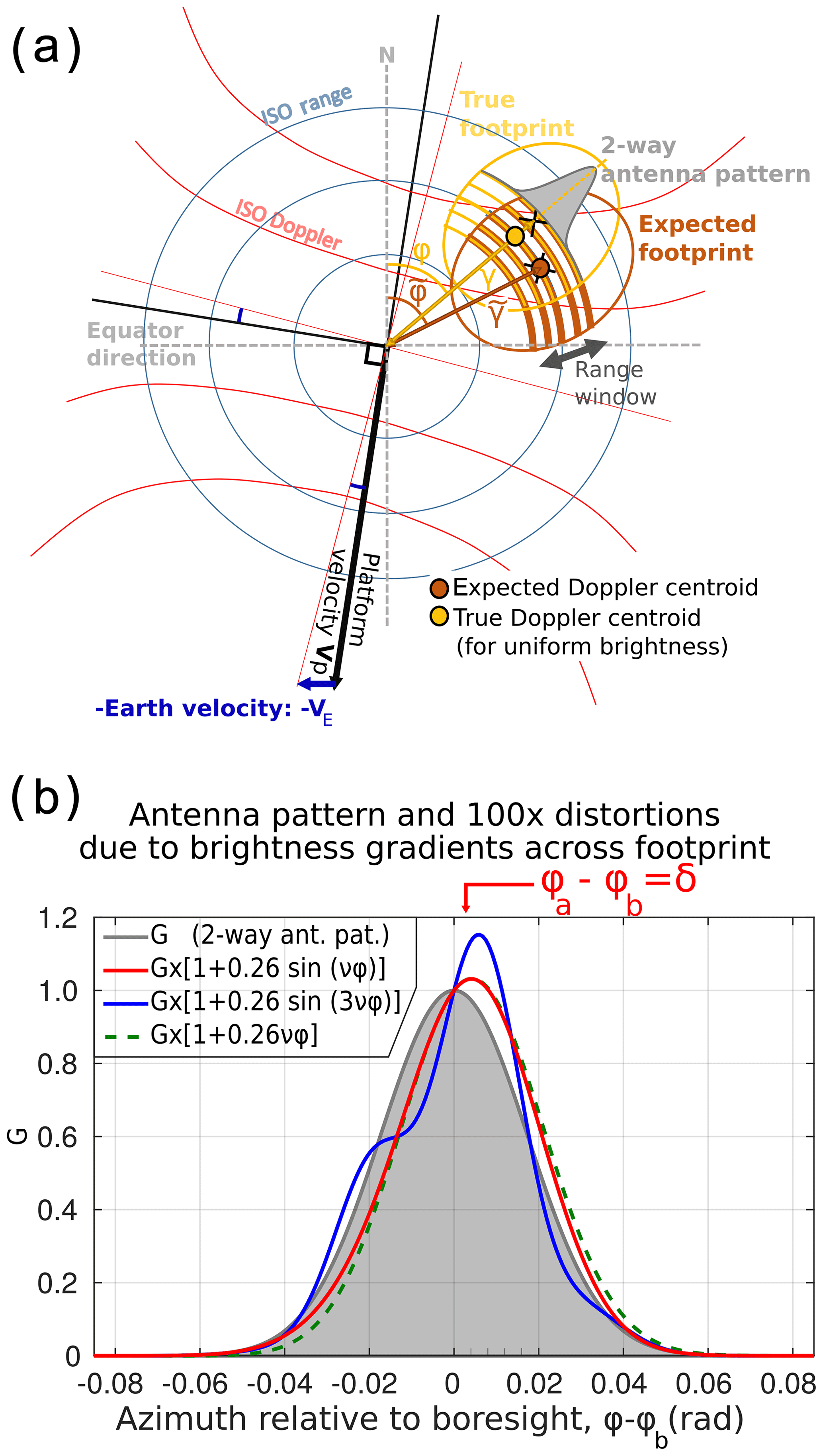
Figure A1(a) True pointing. The attitude drift changes the antenna footprint direction and shifts the DFS centroid. Here γ and φ are the expected coordinates of the antenna gain ground projection, while and are the shifted versions of these coordinates by the attitude misknowledge (adapted from Ardhuin et al., 2019b). (b) Apparent pointing φa for the SKIM geometry. Examples of two-way antenna gain G as a function of azimuth and distortions (exaggerated 100 times) induced by σ0 gradients on the power integrated by the radar in the azimuth direction across the antenna diagram (gray curve). Three examples of asymmetric distortions are given: a sine function with , a sine function varying 3 times faster and a linear trend. Such distortions induce an apparent mispointing of the beam δφ and a correction to the geometrical line-of-sight relative velocity estimate.
Figure A1a shows the measurement geometry seen from above. One can see that uncertainties on the viewing azimuth and incidence angle have different origins.
-
The uncertainty in azimuth can be due to imperfect knowledge of the weighting corresponding to the term in Eq. (A24). This can of course come from imperfect platform attitude or antenna orientation information but also from an imperfect characterization of the antenna radiation diagram or the distribution of σ0 on the sea surface.
-
The uncertainty in incidence angle is due to imperfect knowledge of the radial position of the range-resolution bins (yellow striping of the footprint in Fig. A1a). This can be due to imperfect timing accuracy or to imperfect knowledge of the vertical separation between the instrument and sea surface.
A2.2 Timing and altitude accuracy
For this brief discussion of the effects of timing and altitude accuracy on incidence angle estimation, we consider a single range bin whose “true” range from the radar is r, whose altitude with respect to the radar is H and the incidence angle is θ. In this case . If the radar now suffers from a timing error δr, the instrument will detect a false altitude H−δr but will ascribe to range bin r−δr the signal coming from r. In the meantime, we consider the surface-tracking algorithm to suffer from an error δh and detect the surface at range . The data from this range bin will thus be processed using an angle of incidence
different from the correct value by
Considering δh and δr to be independent, we see that at 12∘ the incidence angle knowledge requirements expressed above for SKIM and KuROS respectively translate to timing accuracy requirements of 36.8 and 7.7 m and to surface-tracking accuracy requirements of 80.4 and 16.9 cm.
The timing accuracy requirements are easily met in the spaceborne context but can be challenging in the cost-constrained context of an airborne instrument.
The surface-tracking algorithm, however, does not benefit from the error compensation that exists for the timing error. The requirement for SKIM is easily met by the nadir altimeter payload of SKIM. The 16.9 cm altitude tracking requirement is out of reach of the KuROS airborne instrument. Our analysis of its DFS data will thus be restricted to the side-looking configurations for which, as per Eq. (A24), the pointing requirements are much milder.
A2.3 Effective pointing and azimuth gradient DFS
As expressed in Eq. (A24), for each range-resolution cell VNG results from an integral over azimuth with a weight that depends on the product of the antenna radiation diagram and the sea surface NRCS, which varies as a function of the horizontal position (x,y) due to the presence of waves, varying winds, currents, surfactants, sea ice and all the physical properties of the sea surface.
Even with perfect knowledge of the platform attitude and velocity, NRCS variations can thus make the effective pointing of the measurements deviate from the pure geometric estimates. Valuable insight into this effect can be gained by considering the saddle-point approximation of Eq. (A24) in the limit of a very narrow antenna diagram (which is clearly applicable for SKIM and KaRADOC, less so for KuROS).
Considering first the case of an antenna pointing towards azimuth φb with an infinitely narrow radiation diagram, we see that the product is well approximated by the Dirac distribution δ(φ−φb). In this limit,
We recognize in this expression Vgeo, the estimate of VNG one would have derived using direct geometric arguments.
The essence of the argument is that the sharpest factor in the integral is the beam radiation diagram. If it is now not infinitely sharp, we see that the effect of a gradient of is to shift the peak of the distribution by an angle
Assuming for a Gaussian approximation,
in which σφ(r′) is a parameter describing the width of the antenna diagram at the working incidence angle, one obtains
with
Alternatively, one can choose to express VNG as the sum of Vgeo, the geometric approximation, plus an azimuth gradient Doppler velocity contribution,
with
and
One can see from these expressions that for a given azimuthal variation of the NRCS the order of magnitude of VAGD is set by the width of the antenna radiation diagram: instruments with a thin diagram, such as SKIM and KaRADOC, are less affected than instruments with a broader diagram, such as KuROS. Also, one sees that VAGD is largest when the instrument looks in the cross-track direction and is zero in the up-track and down-track viewing directions. Finally, one sees that VAGD is equivalent to the line-of-sight projection of a spurious horizontal velocity UAGD, which varies with incidence angle only through the variations of and σφ:
At small scales, spatial gradients add to the azimuthal gradient and also induce a spurious velocity with the same expression as a function of . Using the simple case of a single Fourier component allows one to evaluate the importance of different scales. The azimuthal shift can be obtained as
In the slow variation limit () and Eq. (A36) this expression coincides with Eq. (A31). For faster variations, one sees that the largest disturbance is obtained when . This azimuthal wavenumber is such that the footprint can host a bright and a dark patch, one on either side of the look direction. This configuration creates the largest disturbance for a given value of the brightness contrast ε. δφ in this case is given by
A precise determination of the antenna diagram is necessary for any Doppler application, given the possibly large contribution of pointing error in the estimation of the non-geophysical DFS and the effect of the antenna beamwidth in the spurious azimuth gradient velocity UAGD. A comprehensive strategy has thus been developed for estimating the one-way antenna diagram in amplitude and phase by combining anechoic chamber measurements and verification using the campaign data with a final adjustment of systematic phase shifts in the data. In this section α and β are respectively the latitude and longitude of a set of spherical coordinates centered on the antenna such that the main lobe extends in a longitudinal sector on the Equator , and the rotation axis of the antenna turntable points towards and . With this choice of coordinates the antenna diagram has separable Gaussian dependencies on α and β. In constant-altitude flight, when the antenna points towards φb, and .
B1 Fixed-antenna NRCS correction
The anechoic chamber measurements are very accurate for the antenna alone. However, once integrated into the plane, the antenna diagram is perturbed. This is, for instance, particularly noticeable in the NRCS measurements in rotating mode, wherein a spurious azimuthal pattern could clearly be seen, and for fixed-antenna DFS observations, wherein a “striping” pattern as a function of incidence angle is obvious.
We have thus developed a complementary method that relies on the variations of the plane attitude during maneuvers. Using the plane IMU, we identify the angular coordinates α and β of the nadir and use the measured power to map the antenna diagram (using as a reference point the constant-altitude return power values for each data segment to account for geophysical nadir NRCS variations). The combination of all the flights during the campaign gives the distribution of measured power as a function of α and β, which is shown in Figs. B1 and B2.
The measured distribution is well approximated by a Gaussian shape
Another expression for G(α,β), more suitable for use with the half-power beamwidths α−3 dB and β−3 dB obtained from anechoic chamber measurements, is
The width parameters in these equations are linked by
The parameter values used in this study are collected in Table 1.
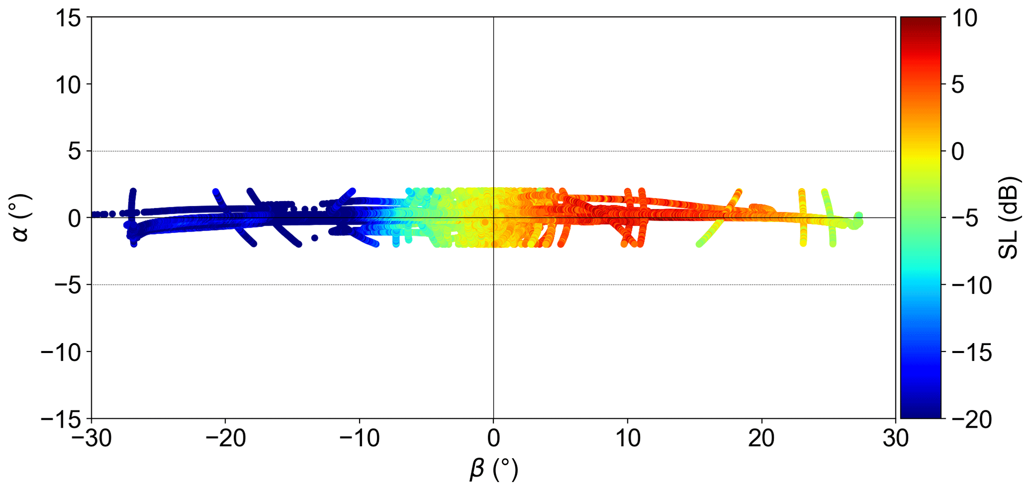
Figure B1Reconstructed α and β dependence of the two-way KuROS antenna diagram. For each 30 s data segment, the constant-altitude values, for which the nadir is at α=0 and β=0, have been used as a reference level to account for geophysical variations in nadir NRCS.

Figure B2Reconstructed azimuth dependence of nadir return power for different incidence angles. For each incidence angle, the α=0 value has been used as a reference. The thick line shows the final Gaussian fit used in the data analysis. The data were excluded from the fit.
One cautionary remark is that the illuminated patch at nadir is not infinitely sharp. The measured distribution is thus the convolution of the true antenna diagram by the power distribution at the nadir patch (which depends on the altitude-tracking error and the sea state; Chelton et al., 1989). Assuming Gaussian shapes, the squares of the width parameters add, leading to
The broadening of the diagram due to finite nadir patch size is thus a small correction provided the scale of the nadir patch remains smaller than the antenna diagram scales. For reasonable orders of magnitude of the altitude-tracking error and significant wave height, the patch −3 dB width is of the order of 3∘ when viewed from 3000 m of height. This corresponds to a 3 % correction on the value of σα. We have chosen to neglect this correction. The values summarized in Table 1 are the parameters of the Gaussian fits to the observed distributions.
B2 Rotating-antenna NRCS correction
Using these parameters as a starting point, we have then constructed corrections for the rotating-antenna measurements of NRCS by allowing the boresight elevation β0 to vary as a function of antenna orientation within the plane. The variation law was determined by minimizing the dependence of the rotating-antenna NRCS measurements as a function of flight direction over the offshore area for each day.
B3 Fixed-antenna DFS correction
In a similar way, we have observed that the KuROS antenna diagram is slightly “wrinkled” in that the beam boresight azimuth changes as a function of elevation. This azimuthal mispointing transposes immediately into a striping modulation of the UGD estimates. A correction was introduced by allowing the boresight azimuth α0 to vary as a function of β. The variation law of α0 was determined by minimizing the average UGD over all flights for each value of β. As the variation of this quantity with respect to α0(β) is not trivial, this required constructing, regularizing and inverting the observation matrix.
KaRADOC is built around an Agilent PNA-X network analyzer, complemented by a TX power amplifier, a T/R switch, an RX low-noise amplifier and a high-gain purpose-built slotted waveguide antenna (shown in Fig. C1).
The beam can be steered in elevation by changing the instrument working frequency (see Fig. C2a), and the antenna is usually mounted on a pitch–roll stabilization platform. For the Drift4SKIM experiment, however, the antenna was rigidly mounted in a port-looking configuration centered on a 10∘ incidence angle with a 2∘ backward-looking tilt to compensate for the aircraft pitch in constant-altitude flight. Plane attitude variations were accounted for in the data processing. Observations were collected at 33.7 GHz, corresponding to a 12∘ nominal incidence angle. Other angles were also scanned, but RF leakage from the TX to the RX subsystems was too strong at the corresponding frequencies, making the signal harder to analyze.
The antenna radiation diagram is very narrow, with a beamwidth less than 1.5∘ in elevation and less than 2∘ in azimuth (see Fig. C2b). Figure C3a represents sections across the KaRADOC main lobe in the azimuth and elevation direction at 33.7 GHz.
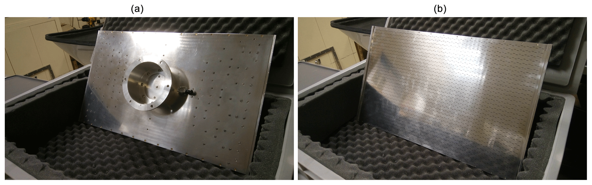
Figure C1The back (a) and front (b) of the antenna.
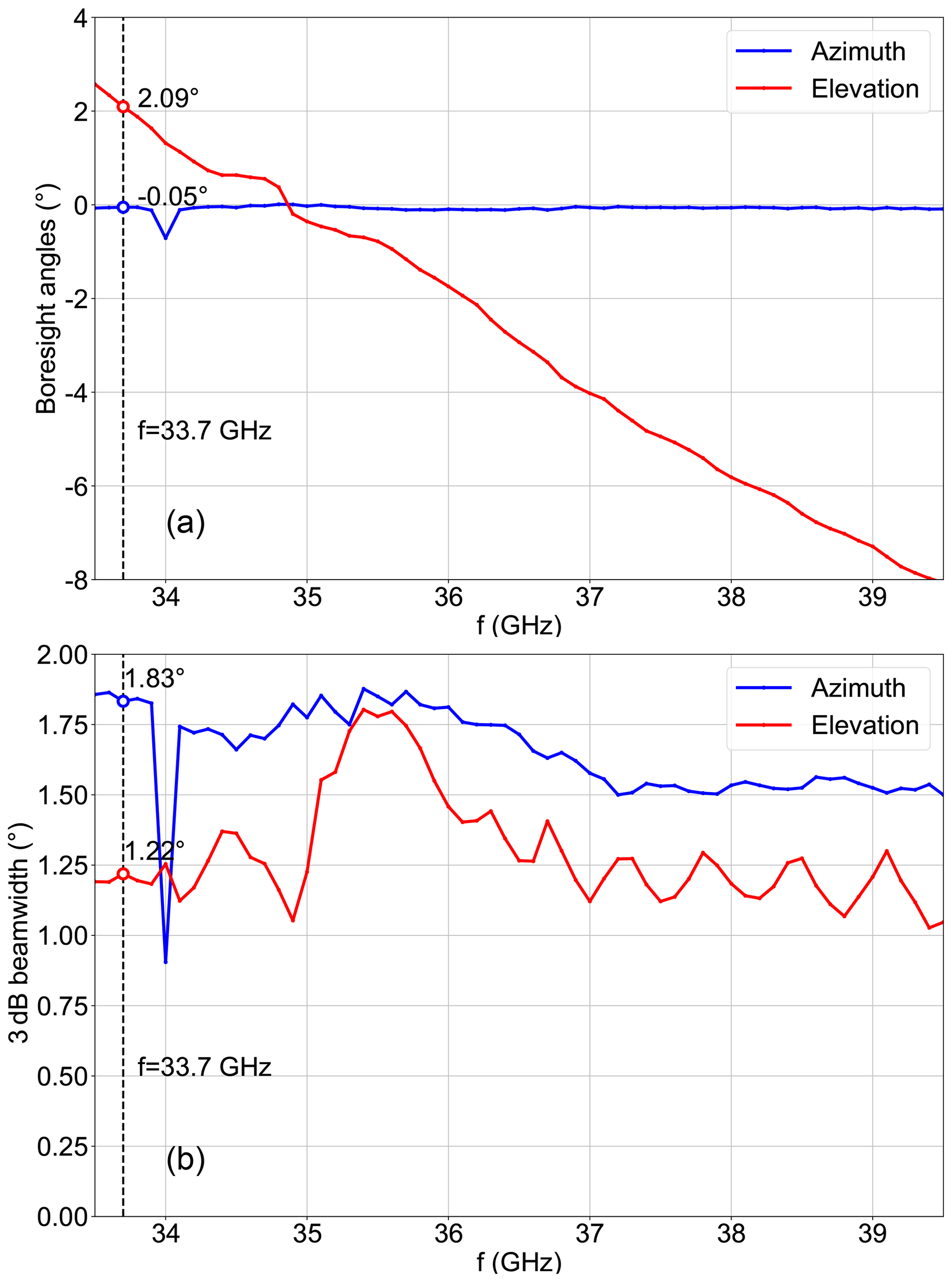
Figure C2Frequency dependence of the KaRADOC main lobe azimuth and elevation boresight angles (a) as well as half-power beamwidths (b).
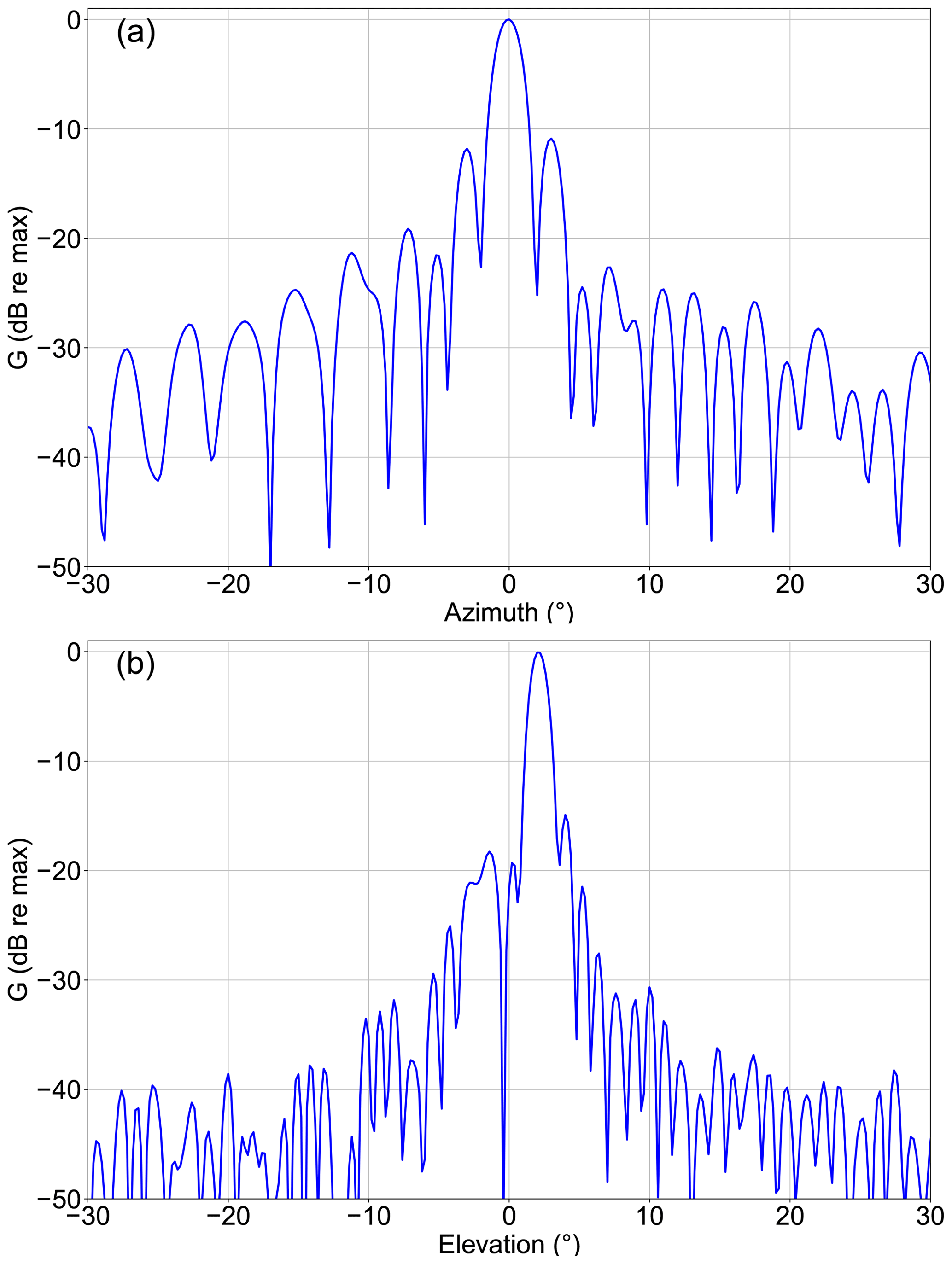
Figure C3KaRADOC radiation diagram at 33.7 GHz as a function of (a) azimuth at 2.09∘ elevation and (b) elevation at −0.05∘ azimuth.
Data and numerical model results presented in this article will be made available on the upcoming website of the ESA-funded IASCO project.
LM, FA, FC, FN, BC, DH, AM, LPG and PS contributed to the preparation of the article. LM, FC, PS, FN, FA, FB, DH, SM, TC, BC and CD contributed to the Drift4SKIM campaign organization and realization. LM, FC, FN, BC, FA, LPG, DH, FB, AM, SM, CP and PS took part in the campaign data analysis. FN, GM and PD contributed to the R3S simulations.
The authors declare that they have no conflict of interest.
The views and opinions expressed in this publication can in no way be taken to reflect the official opinion of the European Space Agency.
The authors wish to thank Erik de Witte at the European Space Agency for his determination and support to the SKIM mission. The in situ measurements owe much to the dedication of the R/V Thalia crew. Airborne data were obtained using the aircraft managed by SAFIRE, the French facility for airborne research, part of the infrastructure of the French National Center for Scientific Research (CNRS), Météo-France and the French National Center for Space Studies (CNES). Many people at LOPS and OceanDataLab also contributed to the preparation, deployment and recovery of the instruments, including Mickael Accensi, Sylvain Herledan, Gilles Guitton, Lucile Gaultier, Michel Hamon, Olivier Péden, Stéphane Leizour and Pierre Branellec. Many people at IETR are involved in the KaRADOC developments: Cécile Leconte, Mohamed Himdi, Paul Leroy, Eric Pottier, and especially Guy Grunfelder and Mor Diama Lo, who made the measurement campaign possible during November 2018. Operation of KuROS during the experiment would not have been possible without the dedication of Christophe Le Gac, Nicolas Pauwels and Christophe Dufour from CNRS/LATMOS. We finally thank Roland Romeiser for his contribution to the online discussion of this article, as well as Ernesto Rodriguez and a second (anonymous) referee for their comments and suggestions, which led to major improvements of this article.
This study was supported by the European Space Agency, through the Drift4SKIM and IASCO contracts (ESA contracts 4000126110/18/NL/FF/gp and 4000129945/19/NL/FF/gp, respectively), and by the Centre National d'Etudes Spatiales (CNES) through the KuROS4SKIM contract.
This paper was edited by John M. Huthnance and reviewed by Ernesto Rodriguez and one anonymous referee.
Ardhuin, F., Marié, L., Rascle, N., Forget, P., and Roland, A.: Observation and estimation of Lagrangian, Stokes and Eulerian currents induced by wind and waves at the sea surface, J. Phys. Oceanogr., 39, 2820–2838, https://doi.org/10.1175/2009JPO4169.1, 2009. a, b, c
Ardhuin, F., Balanche, A., Stutzmann, E., and Obrebski, M.: From seismic noise to ocean wave parameters: general methods and validation, J. Geophys. Res., 117, C05002, https://doi.org/10.1029/2011JC007449, 2012. a
Ardhuin, F., Aksenov, Y., Benetazzo, A., Bertino, L., Brandt, P., Caubet, E., Chapron, B., Collard, F., Cravatte, S., Delouis, J.-M., Dias, F., Dibarboure, G., Gaultier, L., Johannessen, J., Korosov, A., Manucharyan, G., Menemenlis, D., Menendez, M., Monnier, G., Mouche, A., Nouguier, F., Nurser, G., Rampal, P., Reniers, A., Rodriguez, E., Stopa, J., Tison, C., Ubelmann, C., van Sebille, E., and Xie, J.: Measuring currents, ice drift, and waves from space: the Sea surface KInematics Multiscale monitoring (SKIM) concept, Ocean Sci., 14, 337–354, https://doi.org/10.5194/os-14-337-2018, 2018. a
Ardhuin, F., Chapron, B., Maes, C., Romeiser, R., Gommenginger, C., Cravatte, S., Morrow, R., Donlon, C., and Bourassa, M.: Satellite Doppler observations for the motions of the oceans, B. Am. Meterol. Soc., 100, 215–219, https://doi.org/10.1175/BAMS-D-19-0039.1, 2019a. a
Ardhuin, F., Marié, L., Peureux, C., Delouis, J.-M., and Gressani, V.: Estimation of non-geophysical Doppler and wave Doppler, and inversion algorithm for SKIM, Tech. Rep. SKIM-MPRC-TN5-V1.5-LOPS-2019, European Space Agency, Noordwijk, the Netherlands, doi:10.13140/RG.2.2.22907.98081/3, 2019b. a, b
Barrick, D. E., Headrick, J. M., Bogle, R. W., and Crombie, D. D.: Sea backscatter at HF: interpretation and utilization of the echo, Proc. IEEE, 62, 673–680, 1974. a
Beckmann, P. and Spizzichino, A.: The scattering of electromagnetic waves from rough surfaces, Artech House, Norwood, MA, USA, 511 pp., 1987. a
Benoit, M., Frigaard, P., and Schäffer, H. A.: Analysing multidirectional wave spectra: a tentative classification of available methods, in: Proceedings of the 1997 IAHR conference, San Francisco, The Johns Hopkins University Press, Baltimore, 131–158, 1997. a
Buck, C.: An extension to the wide swath ocean altimeter concept, in: Proceedings of the IEEE International Geoscience and Remote Sensing Symposium (IGARSS), 8, 543–5439, https://doi.org/10.1109/IGARSS.2005.1525970, 2005. a
Caudal, G., Hauser, D., Valentin, R., and Gac, C. L.: KuROS: A new airborne Ku-band doppler radar for observation of surfaces, J. Atmos. Ocean Technol., 31, 2023–2245, https://doi.org/10.1175/JTECH-D-14-00013.1, 2014. a, b
Chapron, B., Vandemark, D., and Elfouhaily, T.: On the skewness of the sea slope probability distribution, in: Gas transfer at water surfaces, edited by: Donelan, M. A., Drennan, W. M., Saltzman, E. S., and Wanninkhof, R., Geophys. Monogr. Ser., 127, 59–63, https://doi.org/10.1029/GM127p0059, 2002. a, b
Chapron, B., Collard, F., and Ardhuin, F.: Direct measurements of ocean surface velocity from space: interpretation and validation, J. Geophys. Res., 110, 1–17, https://doi.org/10.1029/2004JC002809, 2005. a, b
Chelton, D. B., Walsh, E. J., and MacArthur, J. L.: Pulse compression and sea level tracking in satellite altimetry, J. Atmos. Ocean Technol., 6, 407–438, https://doi.org/10.1175/1520-0426(1989)006<0407:pcaslt>2.0.co;2, 1989. a
Chelton, D. B., Schlax, M. G., Samelson, R. M., Farrar, J. T., Molemaker, M. J., and Gula, J. C. M. J.: Prospects for future satellite estimation of small-scale variability of ocean surface velocity and vorticity, Prog. Oceanogr., 173, 256–350, https://doi.org/10.1016/j.pocean.2018.10.012, 2019. a, b
Chu, X., He, Y., and Chen, G.: Asymmetry and anisotropy of microwave backscatter at low incidence angles, IEEE Trans. Geosci. Remote Sens., 50, 4014–4024, 2012. a
Crombie, D. D.: Theory of HF ground wave backscatter from sea waves, Nature, 175, 681–682, 1955. a
Elfouhaily, T., Chapron, B., Katsaros, K., and Vandemark, D.: A unified directional spectrum for long and short wind-driven waves, J. Geophys. Res., 102, 15781–15796, https://doi.org/10.1029/97jc00467, 1997. a, b, c, d, e
Elfouhaily, T. M.: A consistent wind and wave model and its application to microwave remote sensing of the ocean surface, Ph.D. thesis, Denis Diderot University, Paris, 1997. a, b, c
ESA: Report for Mission Selection: SKIM, Tech. Rep. ESA-EOPSM-SKIM-RP-3550, European Space Agency, Noordwijk, the Netherlands, https://doi.org/10.13140/RG.2.2.22907.98081/3, 2019. a, b, c, d
Veras Guimarães, P., Ardhuin, F., Sutherland, P., Accensi, M., Hamon, M., Pérignon, Y., Thomson, J., Benetazzo, A., and Ferrant, P.: A surface kinematics buoy (SKIB) for wave–current interaction studies, Ocean Sci., 14, 1449–1460, https://doi.org/10.5194/os-14-1449-2018, 2018. a
Gurgel, K.-W., Antonischki, G., Essen, H.-H., and Schlick, T.: Wellen Radar (WERA), a new ground-wave based HF radar for ocean remote sensing, Coastal Eng., 37, 219–234, https://doi.org/10.1016/S0378-3839(99)00027-7, 1999. a
Hansen, M. W., Johannessen, J. A., Dagestad, K. F., Collard, F., and Chapron, B.: Monitoring the surface inflow of Atlantic Water to the Norwegian Sea using Envisat ASAR, J. Geophys. Res., 116, C12008, https://doi.org/10.1029/2011JC007375, 2011. a
Hauser, D., Tison, C., Amiot, T., Delaye, L., Corcoral, N., and Castillan, P.: SWIM: The first spaceborne wave scatterometer, IEEE Trans. Geosci. Remote Sens., 55, 3000–3014, 2017. a
Hauser, D., Tourain, C., Hermozo, L., Alraddawi, D., Aouf, L., Chapron, B., Dalphinet, A., Delaye, L., Dalila, M., Dormy, E., Gouillon, F., Gressani, V., Grouazel, A., Guitton, G., Husson, R., Mironov, A., Mouche, A., Ollivier, A., Oruba, L., Piras, F., Suquet, R. R., Schippers, P., Tison, C., and Tran, N.: New Observations From the SWIM Radar On-Board CFOSAT: Instrument Validation and Ocean Wave Measurement Assessment, IEEE Trans. Geosci. Remote Sens., 1–22, https://doi.org/10.1109/TGRS.2020.2994372, 2020. a
Jackson, F. C., Walton, W. T., and Baker, P. L.: Aircraft and satellite measurement of ocean wave directional spectra using scanning-beam microwave radars, J. Geophys. Res., 90, 987–1004, 1985. a
Kenyon, K. E.: Stokes drift for random gravity waves, J. Geophys. Res., 74, 6991–6994, 1969. a
Kirby, J. T. and Chen, T.-M.: Surface waves on vertically sheared flows: approximate dispersion relations, J. Geophys. Res., 94, 1013–1027, 1989. a
Lazure, P. and Dumas, F.: An external-internal mode coupling for a 3D hydrodynamical model for applications at regional scale (MARS), Adv. Water Resour., 31, 233–250, 2008. a
Le Boyer, A., Cambon, G., Daniault, N., Herbette, S., Cann, B. L., Marié, L., and Morin, P.: Observations of the Ushant tidal front in September 2007, Cont. Shelf Res., 29, 1026–1037, https://doi.org/10.1016/j.csr.2008.12.020, 2009. a
Lygre, A. and Krogstad, H. E.: Maximum entropy estimation of the directional distribution in ocean wave spectra, J. Phys. Oceanogr., 16, 2052–2060, 1986. a
Martin, A. C. H., Gommenginger, C., Marquez, J., Doody, S., Navarro, V., and Buck, C.: Wind-wave-induced velocity in ATI SAR ocean surface currents: First experimental evidence from an airborne campaign, J. Geophys. Res., 121, 1640–1653, https://doi.org/10.1002/2015JC011459, 2016. a
Martin, A. C. H., Gommenginger, C. P., and Quilfen, Y.: Simultaneous ocean surface current and wind vectors retrieval with squinted SAR interferometry: Geophysical inversion and performance assessment, Remote Sens. Environ., 216, 798–808, https://doi.org/10.1016/j.rse.2018.06.013, 2018. a, b
Munk, W.: An inconvenient sea truth: spread, steepness, and skewness of surface slopes, Annu. Rev. Mar. Sci., 1, 377–415, 2008. a, b
Niiler, P. P. and Paduan, J. D.: Wind-driven motions in the Northeast Pacific as measured by Lagrangian drifters, J. Phys. Oceanogr., 25, 2819–2930, 1995. a
Nouguier, F.: Remote Sensing Spatial Simulator (R3S), Tech. Rep. SKIM-MPRC-TN6-V1.0-LOPS-2019, European Space Agency, Noordwijk, the Netherlands, https://doi.org/10.13140/RG.2.2.21423.97440, 2019. a, b, c, d
Nouguier, F., Guérin, C.-A., and Soriano, G.: Analytical techniques for the Doppler signature of sea surfaces in the microwave regime – I: linear surfaces, IEEE Trans. Geosci. Remote Sens., 49, 4856–4864, https://doi.org/10.1109/TGRS.2011.2152848, 2011. a, b, c
Nouguier, F., Mouche, A., Rascle, N., Chapron, B., and Vandemark, D.: Analysis of dual-frequency ocean backscatter measurements at Ku- and Ka-bands using near-nadir incidence GPM radar data, IEEE Geosci. Remote Sens. Lett., 31, 2023–2245, https://doi.org/10.1109/LGRS.2016.2583198, 2016. a, b
Nouguier, F., Chapron, B., Collard, F., Mouche, A., Rascle, N., Ardhuin, F., and Wu, X.: Sea surface kinematics from near-nadir radar measurements, IEEE Trans. Geosci. Remote Sens., 56, 6169–6179, https://doi.org/10.1109/TGRS.2018.2833200, 2018. a, b, c, d, e, f
Novelli, G., Guigand, C. M., Cousin, C., Ryan, E. H., Laxague, N. J. M., Dai, H., Haus, B. K., and Özgökmen, T. M.: A biodegradable surface drifter for ocean sampling on a massive scale, J. Atmos. Ocean Technol., 34, 2509–2532, https://doi.org/10.1175/JTECH-D-17-0055.1, 2017. a
Peureux, C., Benetazzo, A., and Ardhuin, F.: Note on the directional properties of meter-scale gravity waves, Ocean Sci., 14, 41–52, https://doi.org/10.5194/os-14-41-2018, 2018. a
Raghukumar, K., Chang, G., Spada, F., Jones, C., Janssen, T., and Gans, A.: Performance characteristics of “Spotter”, a newly developed real-time wave measurement buoy, J. Atmos. Ocean. Technol., 36, 1127–1141, https://doi.org/10.1175/JTECH-D-18-0151.1, 2019. a
Redelsperger, J.-L., Bouin, M.-N., Pianezze, J., Garnier, V., and Marié, L.: Impact of a sharp, small-scale SST front on the marine atmospheric boundary layer on the Iroise Sea: Analysis from a hectometric simulation, Q. J. Roy. Meteor. Soc., 145, 3692–3714, https://doi.org/10.1002/qj.3650, 2019. a
Rodriguez, E.: On the optimal design of Doppler scatterometers, Remote Sens., 10, 1765, https://doi.org/10.3390/rs10111765, 2018. a, b, c, d, e
Rodríguez, E., Wineteer, A., Perkovic-Martin, D., Gál, T., Stiles, B. W., Niamsuwan, N., and Monje, R. R.: Estimating ocean vector winds and currents using a Ka-band pencil-beam Doppler scatterometer, Remote Sens., 4, 59 pp., https://doi.org/10.3390/rs10040576, 2018. a, b, c, d, e, f, g, h, i
Roland, A. and Ardhuin, F.: On the developments of spectral wave models: numerics and parameterizations for the coastal ocean, Ocean Dynam., 64, 833–846, https://doi.org/10.1007/s10236-014-0711-z, 2014. a
Romeiser, R., Breit, H., Eineder, M., Runge, H., Flament, P., de Jong, K., and Vogelzang, J.: On the suitability of TerraSAR-X split antenna mode for current measurements by along-track interferometry, in: Proceedings of the IGARSS conference, Toulouse, France, 1320–1322, 2003. a
Rossby, T., Flagg, C. N., Donohue, K., Fontana, S., Curry, R., Andres, M., and Forsyth, J.: Oleander is more than a flower: twenty-five years of oceanography aboard a merchant vessel, Oceanography, 32, 126–137, https://doi.org/10.5670/oceanog.2019.319, 2019. a
Rouault, M. J., Mouche, A., Collard, F., Johannessen, J. A., and Chapron, B.: Mapping the Agulhas Current from space: An assessment of ASAR surface current velocities, J. Geophys. Res., 115, C10026, https://doi.org/10.1029/2009JC006050, 2010. a
Sandwell, D. T. and Smith, W. H. F.: Slope correction for ocean radar altimetry, J. Geodesy, 88, 765–771, https://doi.org/10.1007/s00190-014-0720-1, 2014. a
Sentchev, A., Forget, P., Barbin, Y., and Yaremchuk, M.: Surface circulation in the Iroise Sea (W. Brittany) from high resolution HF radar mapping, J. Mar. Sys., 109–110, S153–S168, https://doi.org/10.1016/j.jmarsys.2011.11.024, 2013. a, b
Stewart, R. H. and Joy, J. W.: HF radio measurements of surface currents, Deep-Sea Res., 21, 1039–1049, 1974. a, b, c
Stopa, J. E., Ardhuin, F., Bababin, A., and Zieger, S.: Comparison and validation of physical wave parameterizations in spectral wave models, Ocean Model., 103, 2–17, https://doi.org/10.1016/j.ocemod.2015.09.003, 2016. a, b, c
Sudre, J., Maes, C., and Garçon, V.: On the global estimates of geostrophic and Ekman surface currents, Limnol. Oceanogr., 3, 1–20, https://doi.org/10.1215/21573689-2071927, 2013. a
Sutherland, G., Marié, L., Reverdin, G., Christensen, K. H., Broström, G., and Ward, B.: Enhanced turbulence associated with the diurnal jet in the ocean surface boundary layer, J. Phys. Oceanogr., 46, 3051–3067, https://doi.org/10.1175/JPO-D-15-0172.1, 2016. a
Sutherland, P., Brozena, J., Rogers, W. E., Doble, M., and Wadhams, P.: Airborne remote sensing of wave propagation in the marginal ice zone, J. Geophys. Res., 123, 4132–4152, https://doi.org/10.1029/2018JC013785, 2018. a
Thomson, J., D’Asaro, E. A., Cronin, M. F., Rogers, W. E., Harcourt, R. R., and Shcherbina, A.: Waves and the equilibrium range at Ocean Weather Station P, J. Geophys. Res., 118, 595–5962, https://doi.org/10.1002/2013JC008837, 2013. a
Walsh, E. J., Hancock, III, D. W., Hines, D. E., Swift, R. N., and Scott, J. F.: An observation of the directional wave spectrum evolution from shoreline to fully developed, J. Phys. Oceanogr., 17, 1288–1295, 1989. a
Walsh, E. J., Banner, M. L., Wright, C. W., Vandemark, D. C., Chapron, B., Jensen, J., and Lee, S.: The Southern Ocean Waves Experiment. Part III: sea surface slope statistics and near-nadir remote sensing, J. Phys. Oceanogr., 38, 670–685, https://doi.org/10.1175/2007JPO3771.1, 2008. a
Yueh, S. H., Tang, W., Fore, A. G., Neumann, G., Hayashi, A., Freedman, A., Chaubell, J., and Lagerloef, G. S. E.: L-Band passive and active microwave geophysical model functions of ocean surface winds and applications to Aquarius retrieval, IEEE Trans. Geosci. Remote Sens., 51, 4619–4632, 2013. a
Yurovsky, Y. Y., Kudryavtsev, V. N., Grodsky, S. A., and Chapron, B.: Sea surface Ka-band doppler measurements: analysis and model development, Remote Sens., 11, 24 pp., https://doi.org/10.3390/rs11070839, 2019. a
Zrnic, D. S.: Spectral moments estimates from correlated pulse pairs, IEEE Trans. Aero. Electronic Sys., 13, 344–354, https://doi.org/10.1109/TAES.1977.308467, 1977. a
- Abstract
- Introduction
- Near-nadir radar Doppler measurements of ocean velocities: theory
- Campaign overview
- Measurements
- Implications for SKIM
- Conclusions and perspectives
- Appendix A: Doppler scatterometry theory
- Appendix B: KuROS antenna diagram determination
- Appendix C: KaRADOC system
- Code and data availability
- Author contributions
- Competing interests
- Disclaimer
- Acknowledgements
- Financial support
- Review statement
- References