Influence of intraseasonal eastern boundary circulation variability on hydrography and biogeochemistry off Peru

The intraseasonal evolution of physical and biogeochemical properties during a coastal trapped wave event off central Peru is analysed using data from an extensive shipboard observational programme conducted between April and June 2017, and remote sensing data. The poleward velocities in the Peru–Chile Undercurrent were highly variable and strongly intensified to above 0.5 m s⁻¹ between the middle and end of May. This intensification was likely caused by a first-baroclinic-mode downwelling coastal trapped wave, excited by a westerly wind anomaly at the Equator and originating at about 95^∘ W. Local winds along the South American coast did not impact the wave. Although there is general agreement between the observed cross-shore-depth velocity structure of the coastal trapped wave and the velocity structure of first vertical mode solution of a linear wave model, there are differences in the details of the two flow distributions. The enhanced poleward flow increased water mass advection from the equatorial current system to the study site. The resulting shorter alongshore transit times between the Equator and the coast off central Peru led to a strong increase in nitrate concentrations, less anoxic water, likely less fixed nitrogen loss to N₂ and a decrease of the nitrogen deficit compared to the situation before the poleward flow intensification. This study highlights the role of changes in the alongshore advection due to coastal trapped waves for the nutrient budget and the cumulative strength of N cycling in the Peruvian oxygen minimum zone. Enhanced availability of nitrate may impact a range of pelagic and benthic elemental cycles, as it represents a major electron acceptor for organic carbon degradation during denitrification and is involved in sulfide oxidation in sediments.

1 Introduction

The Peruvian upwelling system (PUS) is one of the most productive regions in the world's ocean with an economically important fishing industry (e.g. Carr, 2002; Chavez et al., 2008). Located in the eastern tropical South Pacific (ETSP), the high surface productivity of the PUS is most pronounced within a 100 km wide stretch along the Peruvian coast between 4 and 16^∘ S (Pennington et al., 2006). Equatorward winds favour upwelling throughout the year (Bakun and Nelson, 1991; Strub et al., 1998) and enable a supply of nutrients from subsurface waters and benthic boundary layer to the euphotic zone, stimulating high primary productivity (Pennington et al., 2006). Below the surface layer, low-oxygen waters supplied to the PUS and enhanced local oxygen consumption due to remineralization of exported organic matter, leading to the development of a pronounced oxygen minimum zone (OMZ). The core of the OMZ with upper and lower bounds at about 30–200 and 400–500 m depth, respectively, is considered to be functionally anoxic (e.g. Ulloa et al., 2012; Thomsen et al., 2016).

The eastern boundary circulation in the PUS is dominated by the poleward Peru–Chile Undercurrent (PCUC) occupying the upper continental slope and shelf at depths from 50 to 200 m (Fig. 1, e.g. Gunther, 1936; Chaigneau et al., 2013). It carries low-oxygen and high-nutrient equatorial subsurface water (ESSW), which constitutes the main source of the upwelled waters (Silva et al., 2009; Albert et al., 2010). Mean poleward velocities associated with the PCUC are between 0.05 and 0.15 m s⁻¹ (Chaigneau et al., 2013). The origin of its source waters is still under debate. Chaigneau et al. (2013) traced its source waters to the Equatorial Undercurrent supplying the PCUC via the Ecuador–Peru Coastal Current, which flows poleward along the coast between the Equator and 5^∘ S. In contrast, a regional model analysis by Montes et al. (2010) suggests that the source waters of the PCUC originate predominately from the two eastward Southern Subsurface Countercurrents, flowing south of the Equator (Fig. 1). Above the PCUC, upwelling dynamics imply the existence of an equatorward geostrophic surface jet, known as the Peru Coastal Current (e.g. Hill et al., 1998; Kämpf and Chapman, 2016). Additional features of the eastern boundary circulation are the Peru–Chile Current flowing equatorward offshore of the PCUC and the Chile–Peru Deep Coastal Current flowing equatorward below the PCUC (Fig. 1, Strub et al., 1998; Chaigneau et al., 2013).

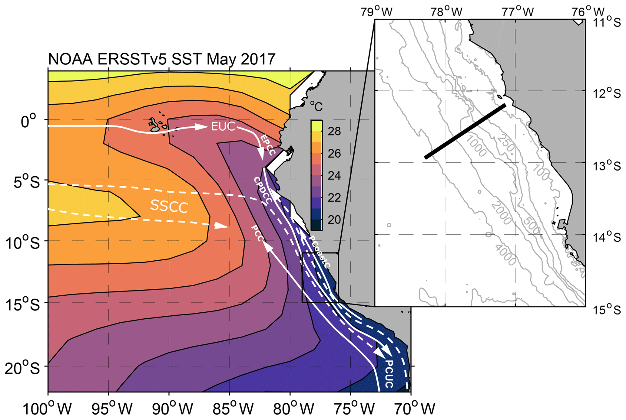
Figure 1 Sea surface temperature (NOAA ERSSTv5 SST) in the eastern tropical Pacific during May 2017 and schematic of the circulation. Solid white lines indicate surface layer currents, while dashed lines indicate thermocline layer currents (after Brandt et al., 2015). Abbreviated currents are the Equatorial Undercurrent (EUC), the Ecuador–Peru Coastal Current (EPCC), the Peru Coastal Current (PCoastC), the Peru–Chile Current (PCC), the two Southern Subsurface Countercurrents (SSCCs), the Chile–Peru Deep Coastal Current (CPDCC) and the Peru–Chile Undercurrent (PCUC). Figure insert shows the position of the 12^∘ S section and local bathymetry (SRTM30 plus topography; Becker et al., 2009).

The PUS exhibits variability on a wide range of timescales, including intraseasonal (e.g. Gutiérrez et al., 2008; Illig et al., 2018a, b), seasonal (e.g. Pizarro et al., 2002) and interannual to decadal (e.g. Graco et al., 2017). Intraseasonal variability of oxygen and nutrient concentrations along the Peruvian margin are known to strongly impact pelagic and benthic ecosystems within the OMZ and the upwelling region above (e.g. Gutiérrez et al., 2008; Echevin et al., 2014; Graco et al., 2017). A prominent benthic example is the response of the biota to oxygenation or deoxygenation episodes with the dominant community changing from macro-invertebrates to bacterial mats (Thioploca/Beggiatoa) during prolonged anoxic episodes (Gutiérrez et al., 2008). Furthermore, in situations where nitrate is present in the anoxic OMZ, anaerobic degradation of organic matter via denitrification can still proceed, while a lack of nitrate favours benthic sulfide emissions, and toxic sulfide plumes in the water column may occur (Schunck et al., 2013; Dale et al., 2016).

A key factor thought to be responsible for the intraseasonal variability of oxygen and nutrient concentrations is the variability of the eastern boundary circulation, forced locally by changes of the wind system above the PUS or forced remotely by variability of the wind system at the Equator. Strengthening (weakening) of the local alongshore winds causes intensified (reduced) Ekman divergence close to the coast that accelerates (decelerates) the coastal surface jet (e.g. Philander and Yoon, 1982; Fennel et al., 2012). Coastal trapped waves (CTWs) are excited and propagate poleward to set up an alongshore pressure gradient balancing an accelerating (decelerating) alongshore flow (Yoon and Philander, 1982). Due to differences in the vertical structure of the surface jet and the excited CTWs, the poleward-flowing PCUC accelerates (decelerates). Furthermore, variability of local wind stress curl forces variability of the poleward undercurrent by affecting the magnitude of Sverdrup transport in the eastern boundary current regime (e.g. McCreary and Chao, 1985; Klenz et al., 2018).

Alternatively, variability of zonal winds in the equatorial Pacific forces equatorial Kelvin waves that propagate eastward. Upon reaching the continental margin, part of their incoming energy is transmitted poleward along the southwestern coast of South America as CTWs (e.g. Moore and Philander, 1977; Enfield et al., 1987). Early measurement programmes off Peru investigating intraseasonal alongshore current variability showed coherent CTW signals with periods of 5–50 d propagating poleward between 5 and 15^∘ S (Brink et al., 1980, 1983; Romea and Smith, 1983). A lack of correlation between coastal tide gauge data and local winds suggested that the CTWs were predominately of equatorial origin. Similarly, intraseasonal CTW variability (50 d period) in the PCUC off Chile with velocity amplitudes of up to 0.7 m s⁻¹ were shown to have originated from wind variability in the central equatorial Pacific (Shaffer et al., 1997). Modelling efforts confirm that equatorially forced intraseasonal CTWs propagate along the eastern South American coast to as far as 30^∘ S (Hormazabal et al., 2002; Illig et al., 2018b).

Poleward propagating CTWs produce vertical displacements of the pycnocline of the order of tens of metres and sea level changes of a few centimetres (Leth and Middleton, 2006; Belmadani et al., 2012). They also modulate the alongshore circulation; that is, CTWs that have a positive sea level anomaly and a downward displacement of the thermocline (downwelling waves) exhibit poleward flow, while CTWs that have a negative sea level anomaly (upwelling waves) exhibit equatorward flow (e.g. Echevin et al., 2014). The combined effect alters the horizontal and vertical supply of nutrients in the PUS. Modelling and satellite observations suggest that subsurface nutrient and chlorophyll intraseasonal variability in the PUS are mainly forced by remotely forced CTWs (Echevin et al., 2014). The simulations indicate that the shoaling and deepening of the nutricline, as well as the horizontal currents associated with the CTW, induce a nutrient flux in and out of the euphotic layer, which impacts primary production. On the other hand, intraseasonal sea surface temperature (SST) variability is suggested to be mainly driven by local winds and heat fluxes, with CTWs playing only a minor role (Dewitte et al., 2011; Illig et al., 2014).

Here, we use an extensive multi-parameter data set from a multi-cruise observational programme to analyse the impact of a strongly elevated and individual propagating CTW on the circulation, hydrography and nutrient concentrations in the PUS. By visiting sampling stations several times over a period of more than 2 months, we measured the variability of the circulation and hydrographic and biogeochemical conditions almost continuously and can distinguish the intraseasonal variability from processes taking place on shorter timescales.

The conditions off Peru in early 2017 were further affected by anomalously warm temperatures in the upper ocean during March associated with a coastal El Niño event (e.g. Garreaud, 2018; Echevin et al., 2018). Our observations cover the declining phase of the coastal El Niño event in April and May when SST anomalies were decreasing.

2 Data

2.1 Ship data

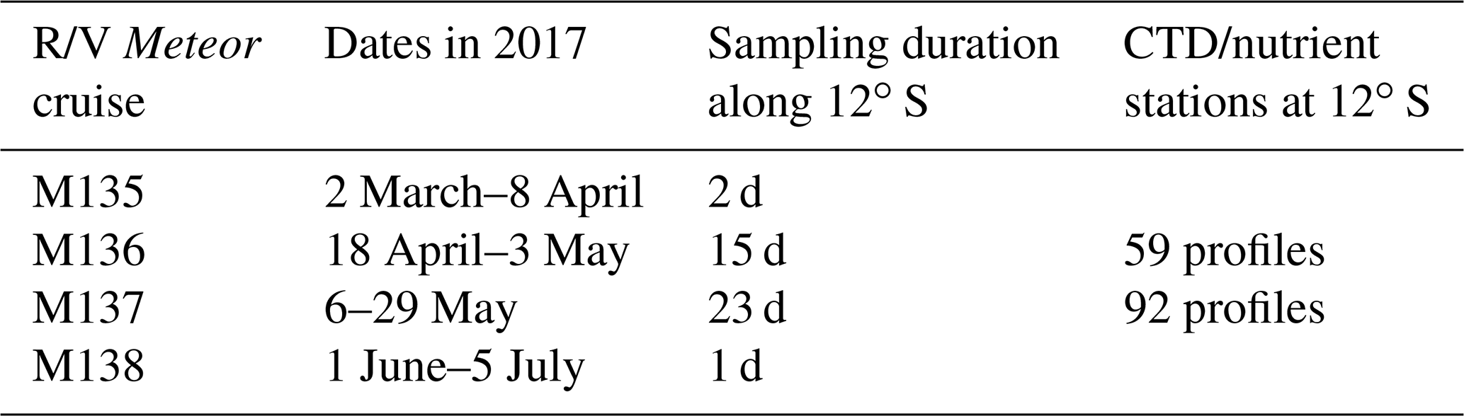
Within the framework of the Collaborative Research Center 754 “Climate-Biogeochemistry Interactions in the Tropical Ocean”, we carried out a combined physical and biogeochemical sampling programme in the ETSP from April to June 2017 during several legs on R/V Meteor (Table 1). A regional focus during the four individual cruises of the sampling programme was a transect starting at shallow waters off Callao (Peru) at about 12^∘ S running offshore perpendicular to the coastline and ends at water depths greater than 5000 m and more than 100 km offshore (Fig. 1). During the first R/V Meteor cruise (M135), the 12^∘ S section was studied towards the end of the cruise (7–8 April). The two subsequent cruises (M136 and M137) focused on benthic and pelagic work off Peru between 11 and 14^∘ S (Dengler and Sommer, 2019; Sommer et al., 2019). Benthic lander measurements required the vessel to remain close to the section between 18 April and 29 May 2017, when repeated hydrographic and velocity measurements along the section were collected. The section was again sampled during the final cruise (M138; 24 June). In this study, we analyse shipboard velocity data and hydrographic profiles, as well as oxygen and nutrient concentration measurements from the repeated measurements along 12^∘ S.

Table 1 Dates of R/V Meteor cruises conducted within the ETSP in 2017 including sampling time and number of conductivity–temperature–depth (CTD) stations collected at 12^∘ S.

2.1.1 Shipboard velocity observations

Upper-ocean velocities were recorded continuously using two vessel-mounted ocean surveyor acoustic Doppler current profiler (vmADCP) systems installed on R/V Meteor. One vmADCP was operated at a frequency of 75 kHz (OS75) and its system configuration during the cruises varied only in depth bin settings. Depth bins of 4, 8 or 16 m were chosen depending on strength of the backscatter signal and the focus of the investigation, allowing a maximum range of 750 m. The second vmADCP operated at 38 kHz (OS38) and recorded depth bins of 32 m while sampling an increased depth range (30–1000 m). During post-processing, vmADCP velocities were corrected using a mean amplitude and misalignment angle determined from water-track calibration (e.g. Fischer et al., 2003). Misalignment angles derived from individual ship accelerations and turns followed a Gaussian distribution having a standard deviation of less than 0.65^∘ for OS75 and less than 0.75^∘ for OS38 (Sommer et al., 2019). A temporal trend was not detectable. The uncertainty of the misalignment angle calibration can be determined from its standard deviation divided by the square root of the number of independent estimates (e.g. Fischer et al., 2003). For our data, more than 100 independent estimates were available for each cruise, resulting in an angle uncertainty of less than 0.1^∘ and an associated velocity bias of less than 1 cm s⁻¹ for underway data. Fischer et al. (2003) suggested an accuracy of 3 cm s⁻¹ for hourly underway data recorded during calm conditions in the tropics.

2.1.2 Hydrographic observations

Along the 12^∘ S section, a total of 151 hydrographic profiles were collected during cruises M136 and M137 with a lowered SeaBird SBE 9-plus conductivity–temperature–depth (CTD) system using double sensor packages for temperature, conductivity and oxygen. The CTD was attached to a General Oceanics rosette with 24 Niskin bottles of 10 L to collect water samples. For the calibration of the conductivity sensor, water samples were analysed with a Guildline Autosal Salinometer model 8400 B. Correction coefficients for the CTD's conductivity sensors were derived using a multi-parameter fit of the Autosal conductivities against the uncalibrated CTD sensor measurements.

CTD oxygen sensors were calibrated against oxygen concentrations determined from bottle water samples using Winkler titration (Winkler, 1888; Grasshoff et al., 1983). Processing and calibration followed the GO-SHIP recommendations (Hood et al., 2010). Previous studies using switchable trace amount oxygen (STOX) sensors have shown that the core of the Peruvian OMZ is functionally anoxic (Revsbech et al., 2009; Thomsen et al., 2016). Unfortunately, the Winkler titration method fails to accurately determine very low oxygen concentrations from bottle water samples. To assure anoxic conditions in the OMZ core, a mean oxygen concentration offset of 2.26 µmol L⁻¹ was subtracted from low oxygen values. Calibration of the salinity and oxygen sensors was performed separately for each cruise, except for M136 where the mean of the calibration of the preceding and succeeding cruises (M135 and M137) was used (M136 lacked deep-water samples required for calibration purposes). The final post-cruise calibration of the data resulted in an accuracy for temperature, salinity and oxygen of 0.002 ^∘C, 0.002 g kg⁻¹ and 1.5 µmol kg⁻¹, respectively.

2.1.3 Nutrient measurements

Water samples collected during the upcast of the CTD rosette were used to determine nutrient concentrations. Concentrations of nitrate, nitrite and phosphate were measured using a QuAAtro autoanalyser (Seal Analytical) with a precision of 0.1, 0.1 and 0.2 µmol L⁻¹, respectively (Sommer et al., 2019). Ammonium concentrations were measured using a fluorimetric method (Holmes et al., 1999).

In addition, concentrations of nitrate were measured using a Satlantic deep Submersible Ultraviolet Nitrate Analyzer (SUNA) mounted on the CTD rosette (Hauschildt et al., 2020). SUNA measurements are based on the absorbance spectra of ultraviolet light (Sakamoto et al., 2009). Data post-processing followed Karstensen et al. (2017) and Thomsen et al. (2019). In a final step, the SUNA nitrate concentrations were calibrated against the nitrate concentrations from the CTD water samples using a linear fit.

2.2 Additional data

Additional regional data sets from satellite observations were used to supplement our analysis of shipboard observations. Sea level anomaly (SLA) data based on satellite altimeter measurements were provided by the EU Copernicus Marine Environmental Monitoring Service (product: SEALEVEL_GLO_PHY_L4_REP_OBSERVATIONS_008 _047). This is a level-4 data set derived by merging all available satellite altimetry data into one gridded product. Reprocessed data from 1 January 1993 to 1 January 2018 with the release days 15 January 2018 (data before 15 May 2017) and 16 May 2018 were accessed. Additionally, sea surface temperature from the NOAA Extended Reconstructed Sea Surface Temperature version 5 (ERSSTv5) data set (Huang et al., 2017a) was analysed. This data set provides monthly values of SST on a $\mathrm{2}{}^{\circ }\times \mathrm{2}{}^{\circ }$ grid based on in situ temperature observations from several sources (Huang et al., 2017b). Finally, wind stress data from the Advanced Scatterometer (ASCAT) product of satellite scatterometer winds (Bentamy and Fillon, 2012) were analysed. This product provides daily global winds and wind stress data with a resolution of 0.25^∘.

3 Methods

3.1 Analysis of velocity observations

The continuous velocity recording was split into segments when the ship was moving in on- or offshore directions only. The velocities were rotated to derive the alongshore component and then a mean velocity section was calculated for each segment of the cruise in 2 km bins according to offshore distance. Periods where the ship was moving slower than 1 kn were excluded. To derive the sections of alongshore velocity over longer time periods, the data from several of these segments were averaged. The presented sections were smoothed using a 2-D Gaussian weights.

3.2 Analysis of hydrographic and biogeochemical data

The analysis of hydrographic data was based on the TEOS10 definitions. Conservative temperature, absolute salinity, density and potential density anomalies were calculated with the Matlab Gibbs Seawater Toolbox (version 3.05; McDougall and Barker, 2011). Nutrient concentrations were transformed to µmol kg⁻¹ to remove the effect of compressibility on vertical gradients. In the following, we use “temperature” to refer to conservative temperature and use “salinity” to refer to absolute salinity.

3.2.1 Nitrogen deficit

In suboxic environments, microbially mediated processes such as denitrification and anaerobic ammonium oxidation (anammox) transform biologically available reactive nitrogen (nitrate, nitrite and ammonium) via intermediate steps into dinitrogen (N₂), which cannot be used by most organisms. These processes lead to a loss of reactive nitrogen relative to other nutrients such as phosphate (${\mathrm{PO}}_{\mathrm{4}}^{\mathrm{3}-}$). The global distribution of nitrate, phosphate and dissolved inorganic carbon (DIC) displays a strong covariation, with the slope of N:P of about 16:1 reflecting the mean stoichiometry of organic matter synthesis and degradation. In order to analyse the impact of nitrogen loss and N₂ fixation on the ${\mathrm{NO}}_{\mathrm{3}}^{-}$ distribution, it is convenient to remove the photosynthesis/remineralization trend and only focus on deviations, N_def, from this trend. The concept of N_def has been introduced (Gruber and Sarmiento, 1997, 2002). Here, the formulation of Chang et al. (2010) was applied to investigate N_def (µmol kg⁻¹). It is based on the deviation from the ratio between nitrogen species and phosphate outside of the eastern tropical South Pacific OMZ and is calculated as

$$\begin{array}{}\text{(1)}& N_{\mathrm{def}}=\mathrm{15.8}({\mathrm{PO}}_{\mathrm{4}}^{\mathrm{3}-}-\mathrm{0.3})-({\mathrm{NO}}_{\mathrm{3}}^{-}+{\mathrm{NO}}_{\mathrm{2}}^{-}+{\mathrm{NH}}_{\mathrm{4}}^{+}),\end{array}$$

where ${\mathrm{PO}}_{\mathrm{4}}^{\mathrm{3}-}$, ${\mathrm{NO}}_{\mathrm{3}}^{-}$, ${\mathrm{NO}}_{\mathrm{2}}^{-}$ and ${\mathrm{NH}}_{\mathrm{4}}^{+}$ are the concentrations of phosphate, nitrate, nitrite and ammonium, respectively. With this definition, positive values of N_def quantify an N loss that has occurred within a certain water mass while it remained in the Peruvian OMZ.

3.2.2 Section averaging

Smoothed hydrographic and biogeochemical properties along the 12^∘ S section were calculated by interpolating the data vertically onto common potential density surfaces. Averaging in density space removes the effect of signal smearing due to vertical displacement caused by internal waves. The profiles were then averaged in bins of 2 km according to distance from the coastline and then smoothed using 2-D Gaussian weights. In a final step, the averaged and smoothed sections were vertically transformed back into depth space using the smoothed depth–density relation.

3.3 Sea level anomaly and wind data

The local SLA along the 12^∘ S section was calculated by first averaging all daily gridded SLA data between 12 and 12.5^∘ S over the time periods used for the velocity sections and interpolating them onto the section according to the distance to the coast. Grid points closer than 30 km to the coast were excluded. Then the mean SLA along the section was subtracted to focus on the cross-shore gradient. In addition, intraseasonal variability along the Equator and coastline was analysed by subtracting the mean SLA over the 25-year time series before bandpass filtering SLA using a fourth-order Butterworth filter for a time window between 20 and 90 d. To follow intraseasonal SLA variability due to propagating waves along the Equator and subsequently along the western South American coast, we used bandpass-filtered SLA data averaged between 0.25^∘ S and 0.25^∘ N from the Equator and two-grid-point averages from near the coast.

For investigating wind forcing of Kelvin waves at the Equator, SLA and zonal wind anomaly were averaged to 5 d means over 10^∘ of longitude. Additionally, wind anomaly was averaged between 5^∘ N and 5^∘ S, while SLA was averaged between 2^∘ N and 2^∘ S.

3.4 Theoretical coastal trapped wave structure

To interpret the observed flow variability along the Peruvian coast in terms of CTWs, the cross-shore-depth structure of CTWs was determined by considering the linear, hydrostatic, inviscid and Boussinesq approximated equations of motion on an f plane using local bathymetry and stratification (Brink, 1982, 1989; Illig et al., 2018a). For alongshore scales larger than cross-shore scales and horizontally uniform stratification, cross-shore-vertical mode structures (eigenfunctions) and corresponding phase velocity (eigenvalue) solutions were obtained from the simplified set of equations by using a resonance iteration approach (Brink, 1982; Brink and Chapman, 1987). Here, we obtained the eigenfunctions and eigenvalues for the first three modes by applying a modified version of the Brink and Chapman (1987) CTW programmes as published by Brink (2018).

Local bathymetry and stratification are required as input to Brink's (2018) set of Matlab mfiles. The cross-shore distribution of bathymetry was taken from the multi-beam echo sounder data collected during the cruises along 12^∘ S. Echo sounder data were averaged in 5 km bins which resulted in a monotonic increase of water depth in the offshore direction. The maximum water depth used for the wave solutions was 5000 m. From two offshore CTD profiles (M136 no. 60 and M137 no. 92) exceeding 3000 m depth, a stratification profile was calculated first for each profile using 20 data points with 1 dbar spacing, and then a mean profile was calculated from both casts in 5 m intervals.

4 Results

4.1 Variability of the boundary circulation

The direct velocity observations from the multi-cruise programme allowed a detailed assessment of the variability of the eastern boundary alongshore velocity structure at 12^∘ S for a period of more than 11 weeks (Fig. 2). During the observational period from early April to 24 June (2017), we captured an event of strongly increased poleward flow that started in early May and lasted for about 35 d.

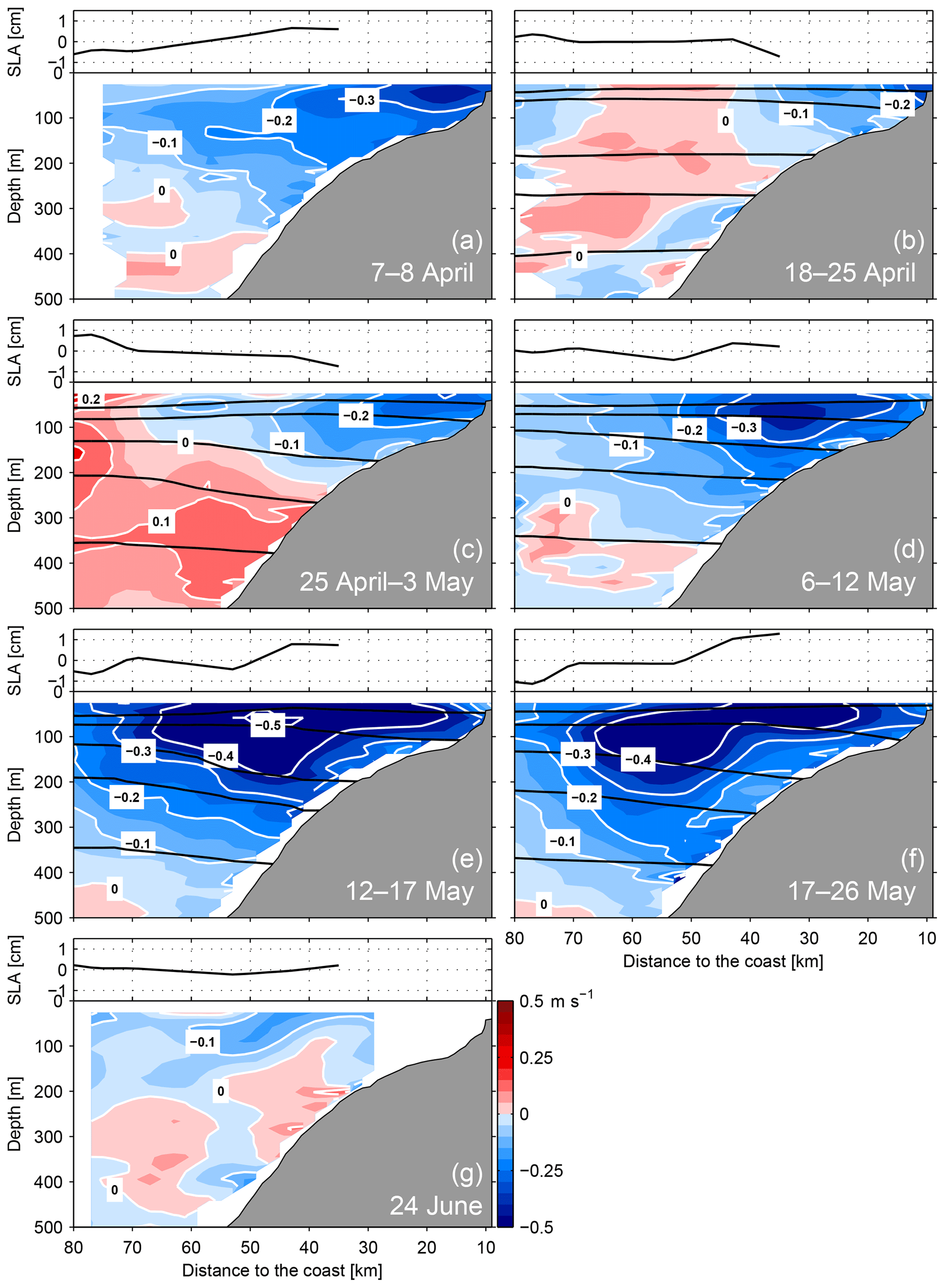
Figure 2 Depth–distance distribution of alongshore velocity (in m s⁻¹, positive equatorward, coloured contour plots) and sea level anomaly (in cm, black line in panel above contour plots) at 12^∘ S during 7–8 April (a), 18–25 April (b), 25 April–3 May (c), 6–12 May (d), 12–17 May (e), 17–26 May (f) and 24 June 2017 (g). Black lines indicate the distribution of isopycnals (σ_θ) at 25.6, 25.9, 26.2, 26.4 and 26.7 kg m⁻³.

The time series started with 2 d of sampling from 7 to 8 April. During this period, a distinct poleward-flowing PCUC was present that extended 80 km offshore (Fig. 2a) and had maximum velocities of more than 0.3 m s⁻¹ on the continental shelf. Satellite altimetry indicated an increasing SLA towards the coast (Fig. 2a). Between 18 April and 26 May, and except for a short break from 4 to 6 May, the 12^∘ S section was continuously surveyed. In mid-April, a poleward flow was present only on the shelf (Fig. 2b). However, from the end of April to mid-May, the PCUC considerably strengthened, reaching maximum core velocities of about 0.5 m s⁻¹ between 50 and 100 m depth 50 km offshore (Fig. 2c–e). Furthermore, the PCUC poleward flow extended to more than 80 km offshore and occupied the water column above 400 m depth. The SLA increased towards the coast (by 2 cm over 40 km), implying that a poleward geostrophic velocity anomaly was present at the sea surface as well. Towards the end of May, poleward flow in the PCUC did not increase further but remained at a similar level as during mid-May (Fig. 2f). In contrast, velocity data from a final section occupation 3 weeks later on 24 June show evidence that the PCUC had weakened drastically (Fig. 2g), exhibiting a comparable velocity distribution as for the period 18–25 April (Fig. 2b). Assuming similar timescales for its deceleration as for its acceleration, the period of intensified PCUC flow was between 30 to 40 d. The intensified PCUC flow strongly exceeded the climatological PCUC flow reported from this region. Mean alongshore flow at 12^∘ S determined from vmADCP data sampled during 22 cruises showed maximum PCUC core velocities of 0.1–0.15 m s⁻¹ (Chaigneau et al., 2013), similar to the situation observed during 18–25 April and 24 June (Fig. 2b and g).

In April, the velocity sections indicated an equatorward flow offshore and below the PCUC (Fig. 2). The Peru Coastal Current and the Chile–Peru Deep Coastal Current are thought to be located at these depths and offshore ranges (e.g. Penven et al., 2005; Chaigneau et al., 2013). In late April, the equatorward flow increased in strength and extended to shallower depths (Fig. 2b and c). However, during the period of strong poleward flow in May, the equatorward flow decreased and was present only below 400 m depth close to the offshore end of the section (Fig. 2e and f). On 24 June, a weak equatorward flow was present below 200 m at most parts of the section but never reached velocities of 0.1 m s⁻¹. We found no indication of equatorward flow above or inshore of the PCUC, where the equatorward surface jet is expected to be situated. The lack of this surface flow in observations was also noted by Chaigneau et al. (2013).

To compare the alongshore circulation with hydrographic and biogeochemical sampling, the data were averaged into two periods: the initial phase of weak poleward flow (Fig. 3a) covering the period of 18 April–3 May and a period of enhanced poleward flow during 12–26 May (Fig. 3b). The increase in poleward velocities was especially strong between 40 and 60 km offshore where velocities increased from about zero to 0.4 m s⁻¹ (Fig. 3c). The core of velocity increase extended deeper than the intensified PCUC and was more detached from the coast.

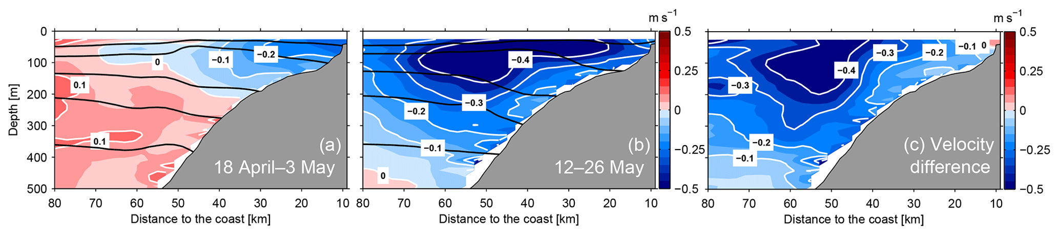
Figure 3 Depth–distance distribution of averaged alongshore velocity (positive equatorward) at 12^∘ S prior to (a, 18 April–3 May 2017) and during (b, 12–26 May 2017) the PCUC intensification period. Panel (c) depicts the velocity difference between the two situations. Black lines indicate the distribution of isopycnals (σ_θ) at 25.6, 25.9, 26.2, 26.4 and 26.7 kg m⁻³.

4.2 Potential causes of circulation variability

4.2.1 Role of local wind stress

Changes in the local wind stress curl are a potential local forcing mechanism of an intensified PCUC flow. An increase in the magnitude of near-coastal negative wind stress curl leads to an increased poleward flow along the eastern boundary through Sverdrup dynamics (e.g. Marchesiello et al., 2003). The adjustment of the circulation to changes in the wind stress curl at the eastern boundary is rather fast and occurs within a few days (Klenz et al., 2018). Wind stress curl along the Peruvian continental margin between 10 and 14^∘ S was negative throughout the observational period (Fig. 4), continuously forcing poleward flow. However, during the period of PCUC acceleration between the end of April and mid-May, the magnitude of negative wind stress curl decreased (Fig. 4c–f). It can thus be ruled out that local wind stress curl forcing is responsible for the observed intensified PCUC. Nevertheless, elevated negative wind stress curl was observed from 18 to 22 May, which may have contributed to maintain a strong PCUC in late May.

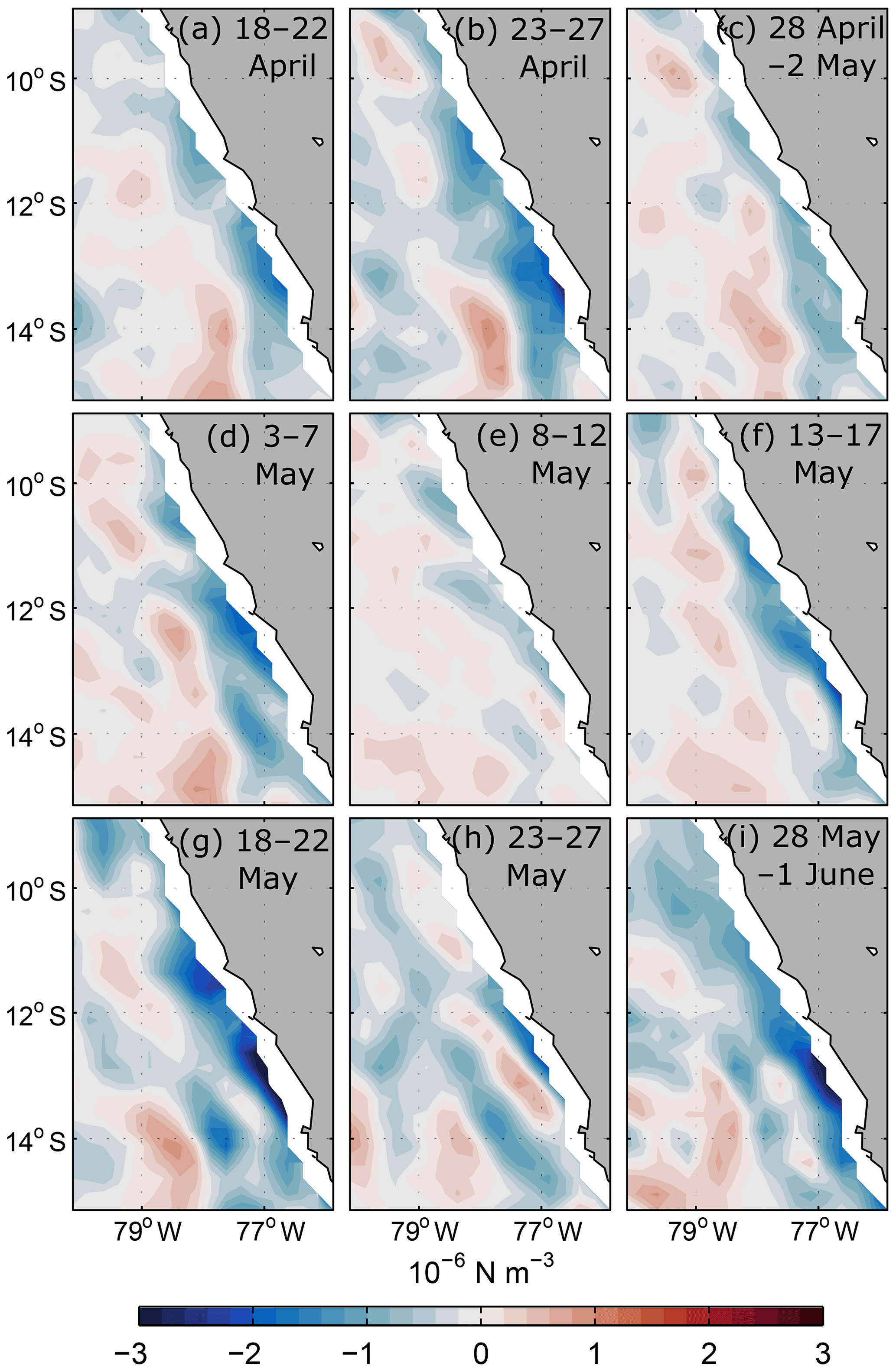
Figure 4 The 5 d mean wind stress curl from ASCAT scatterometer winds off Peru during 18–22 April (a), 23–27 April (b), 28 April–2 May (c), 3–7 May (d), 8–12 May (e), 13–17 May (f), 18–22 May (g), 23–27 May (h) and 28 May–1 June 2017 (i).

Variability of near-coastal alongshore wind stress excites CTWs that propagate poleward (e.g. Yoon and Philander, 1982) and thereby enhances or decreases poleward flow within the depth range of the PCUC. From mid-April to May 2017, alongshore wind stress between 6 and 15^∘ S was variable (Fig. 5). While moderate wind stress (0.03–0.06 N m⁻²) prevailed from mid-April to 3 May, it was weak during the first 2 weeks of May (Fig. 5d, e, g). On 15 May, the wind stress increased and remained elevated for a period of about 5 d. This wind variability cannot explain the observed changes in poleward transport. The poleward transport increased from late April to its maximum mid-May, whereas the alongshore wind stress during this period decreased in the first week and then increased 7 d later.

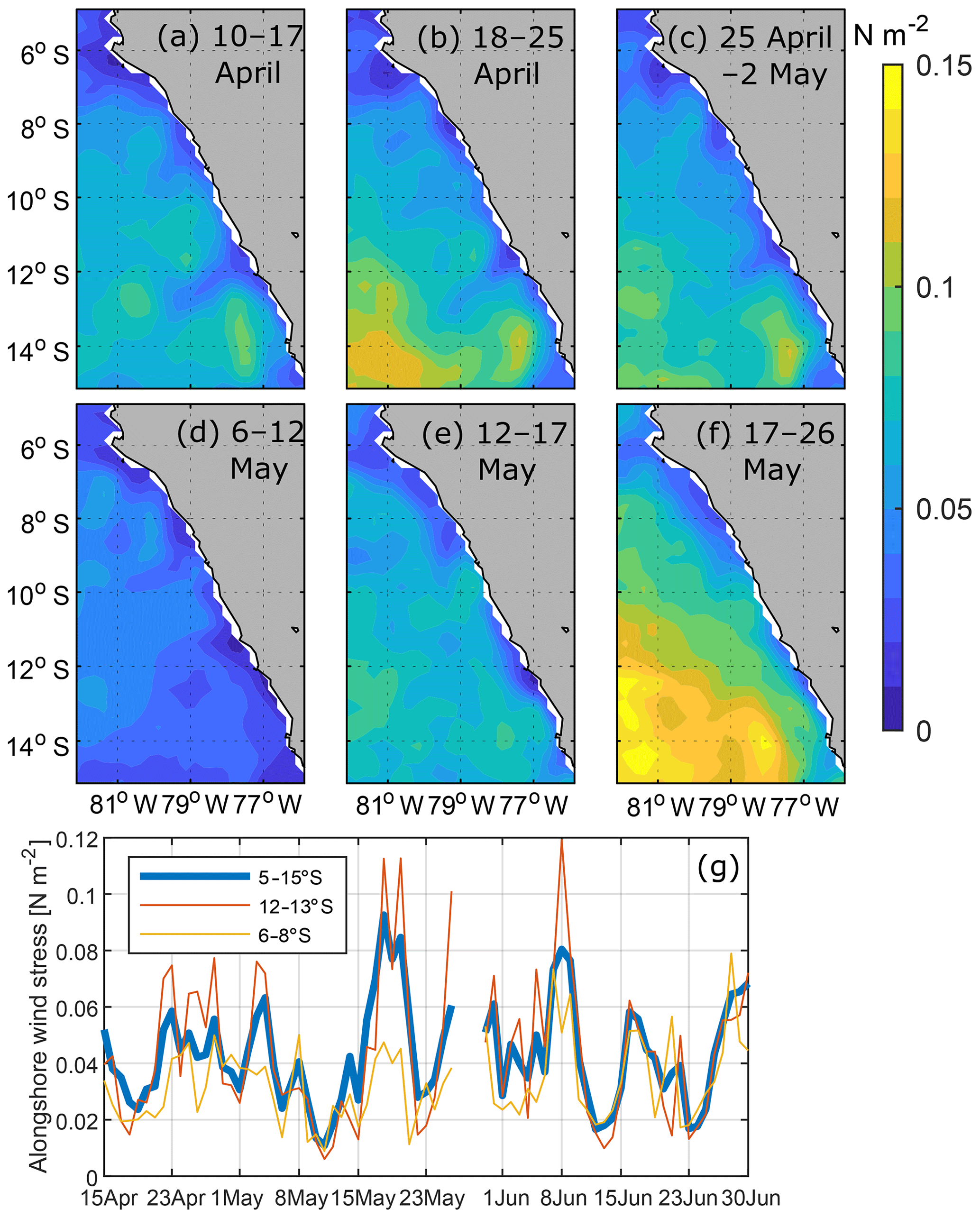
Figure 5 Alongshore wind stress from ASCAT scatterometer winds (a–f) averaged over 10–17 April (a), 18–25 April (b), 25 April–2 May (c), 6–12 May (d), 12–17 May (e) and 17–26 May (f). Panel (g) shows time series of alongshore wind stress averaged between 30 and 80 km from the coast for different bands of latitude.

4.2.2 Equatorial winds and wave response

According to equatorial linear wave theory a weakening of the trade winds at the Equator by, e.g. westerly wind events, generates an eastward propagating equatorial Kelvin wave. Once the equatorial Kelvin wave interacts with the eastern boundary, parts of its energy are transmitted to a CTW (Enfield et al., 1987). Indeed, several westerly wind anomalies occurred in the central and eastern equatorial Pacific during the first 6 months of 2017 (Fig. 6). A particularly elevated westerly wind anomaly occurred between the International Date Line and 120^∘ W during the first 2 weeks of April (Fig. 6a). In response, a positive SLA propagating along the Equator appeared to the east of the wind event between about 100 and 80^∘ W (Fig. 6b, dash line, Fig. 7) and arrived at the eastern boundary at the beginning of May.

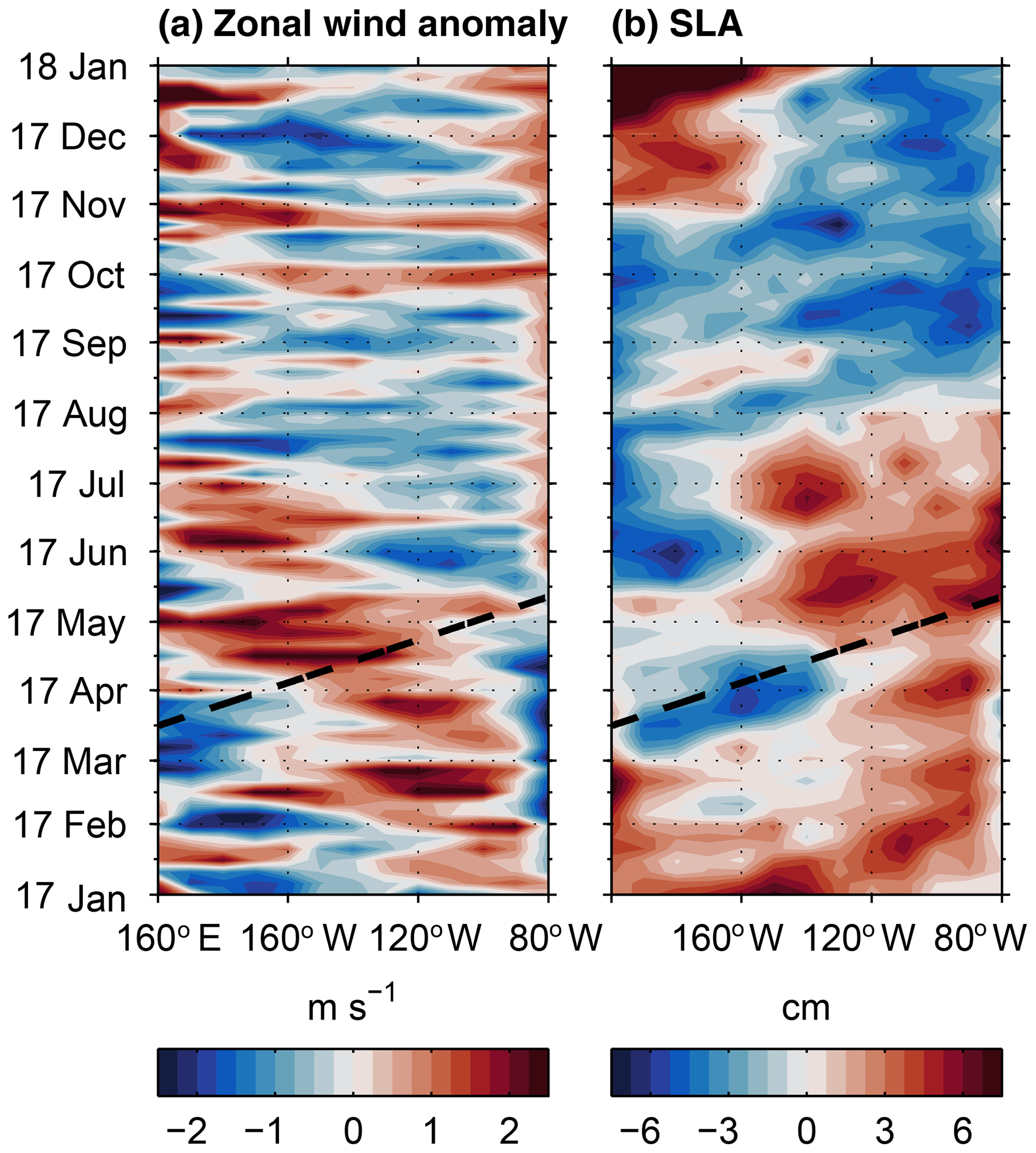
Figure 6 Hovmöller diagram of zonal wind anomaly (a) and SLA (b) along the central and eastern equatorial Pacific for the year 2017. The propagation of a first-mode equatorial Kelvin wave is indicated by the dashed black line (phase speed 2.7 m s⁻¹; Yu and McPhaden, 1999).

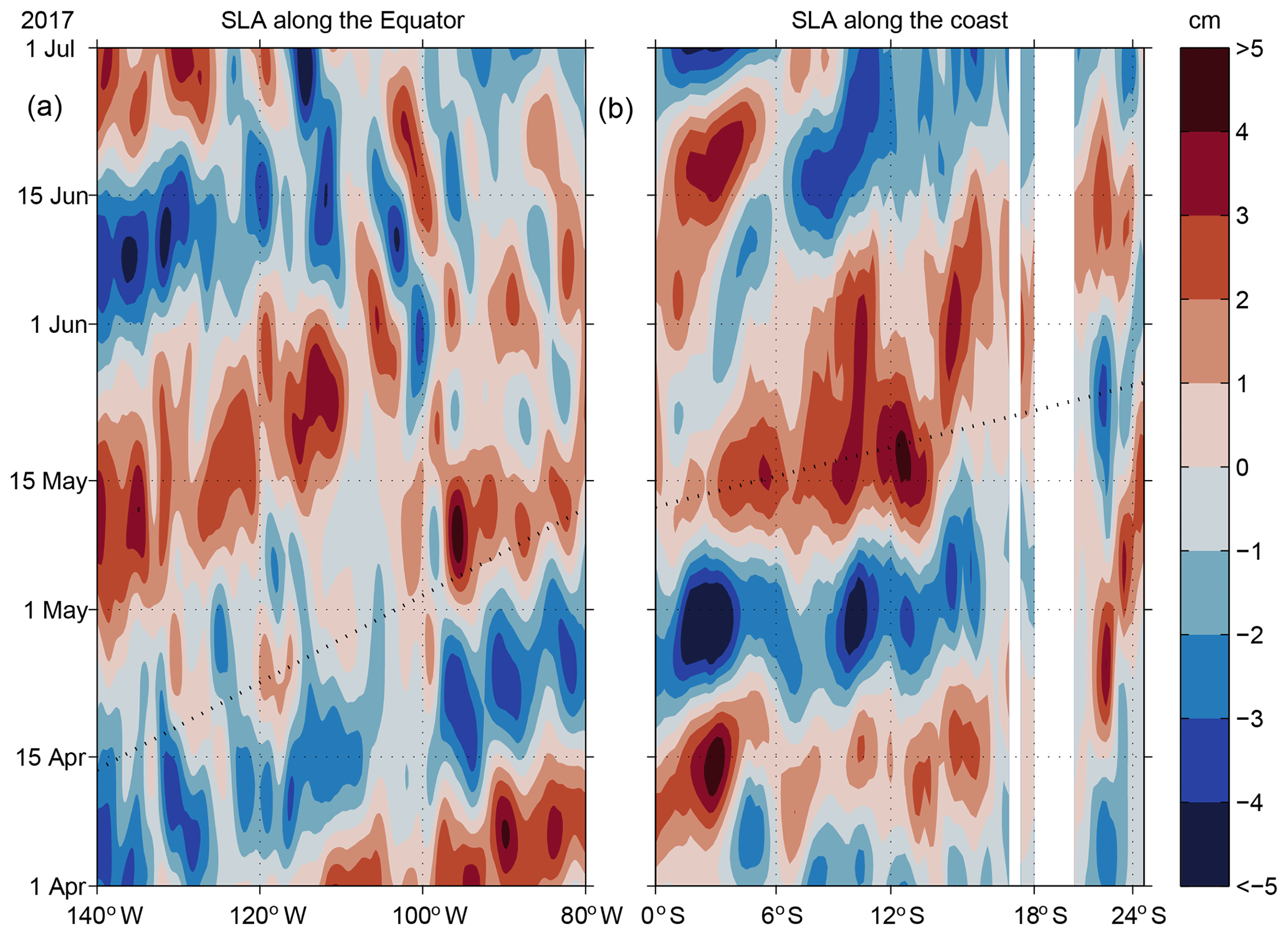
Figure 7 Bandpass-filtered (20–90 d) sea level anomaly along the eastern equatorial Pacific averaged between 0.25^∘ N and 0.25^∘ S (a) and along the western coast of South America (b) averaged over the two grid points closest to the coastline. The propagation of a first-mode equatorial Kelvin wave and CTW are shown as dotted black lines; the phase speed of the equatorial wave is 2.7 m s⁻¹ (Yu and McPhaden, 1999) and 3.1 m s⁻¹ for CTWs (see Fig. 8b).

Bandpass-filtered SLA data from the Equator and from near the continental slope (Sect. 3.3) along the South American continent (Fig. 7) indicate that the positive SLA arriving at the eastern boundary continued southward along the eastern boundary to about 14^∘ S. Along the Equator, the propagation speed of the SLA was about 2.7 m s⁻¹ (dashed line in Fig. 7a), which agrees with the phase speed of a first vertical mode equatorial Kelvin wave (e.g. Yu and McPhaden, 1999). The speed of propagation of the SLA signal along the eastern boundary was somewhat enhanced and around 3 m s⁻¹. A positive SLA signal was associated with a negative (downward) displacement of the thermocline, eastward upper-ocean velocities at the Equator and poleward upper-ocean velocities at the continental slope. This agrees well with the SLA signal and the increased poleward PCUC velocities at 12^∘ S and suggests the existence of a downwelling CTW during May 2017.

4.2.3 Modal structure of the intensified flow

To further investigate the nature of the boundary flow intensification, the cross-shore-depth structure of alongshore velocity was determined for the first three CTW modes at 12^∘ S (Fig. 8; see Sect. 3.4 for a description of the model used). Due to a steep continental slope at 12^∘ S, the velocity structure of the different CTW solutions varied predominately in the vertical axis with poles of opposing velocity located above each other (Fig. 8). Flow reversal for each individual mode away from the boundary occurs at shallower depth compared to inshore regions. Higher modes exhibit an upper pole of enhanced velocity located at shallower depth compared to lower modes.

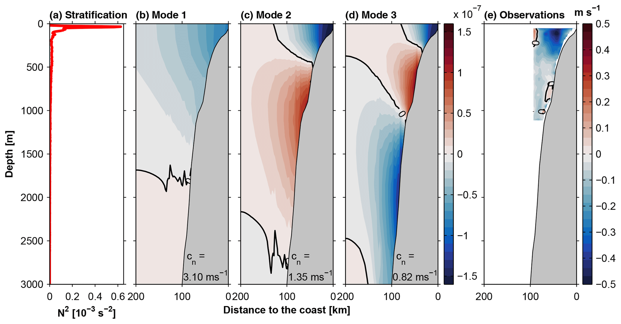
Figure 8 Profile of stratification (N²) (a) and cross-shore-depth structure of alongshore velocity (arbitrary amplitude) obtained for the first three CTW modes (b–d). Panel (e) shows the difference of observed alongshore velocity between 18 April–3 May and 12–26 May 2017. Note that the CTW phase speeds c_n are given in the lower right corner of the respective velocity structure panel.

For comparison, Fig. 8e shows the difference of full-depth low-frequency vmADCP alongshore velocities between 12–26 May and 18 April–3 May. Apart from the increased poleward velocity in the upper 500 m, the alongshore velocity difference resolved by OS38 was weakly poleward throughout the upper 1000 m of the water column (Fig. 8e). Comparing the baroclinic structure of the observations to the baroclinic structure of the different CTW modes, the missing flow reversal in the upper 1000 m shows that the observed change in alongshore velocity is best described by a first-mode CTW. This mode features poleward flow anomalies throughout the upper 1500 m (Fig. 8b) which agrees with the distribution of the velocity differences between the two time periods throughout most of the upper 1000 m (Fig. 8e). The maximum increase of poleward flow, on the other hand, was restricted to a depth range similar to the upper poleward velocity core of a second-mode CTW.

Additional support for the presence of a first-mode CTW originates from a comparison of the phase speeds. At 12^∘ S, the local phase speeds of the model CTW modes (Fig. 8) were higher than those for equatorial Kelvin waves. In particular, the phase speed of the first-mode CTW was 3.1 m s⁻¹, which agrees very well with the phase propagation of the SLA signal discussed in Sect. 4.2.2.

4.3 Response of hydrographic conditions to the PCUC intensification

In the following, we analyse the changes in hydrographic conditions co-occurring with the increase of the alongshore flow. Lower near-surface temperatures near the coast compared to offshore (Figs. 1, 9a and b) indicated active upwelling during the observational programme. While the upwelling signal was restricted to the upper 50 m, near-coastal water masses between 50 and 300 m were significantly warmer compared to water masses offshore (Fig. 9a). During the intensified PCUC period (Fig. 9b, e, h), the cross-shore temperature gradient intensified, leading to an increased downward displacement of isopycnals and isotherms near the coast (Fig. 9b). There, the associated warming signal between 100 and 200 m depth was up to 0.5 ^∘C. Note that during the PCUC intensified period, near-coastal surface temperatures decreased.

Salinity featured a shallow subsurface salinity maximum at about 25 m depth originating offshore and extending over the slope and shelf (Fig. 9d and e). As for temperature, cross-shore salinity gradients were evident between 50 and 300 m depth with higher salinities near the coast which intensified when the PCUC increased. At the same time, salinity at the upper shelf decreased (Fig. 9f).

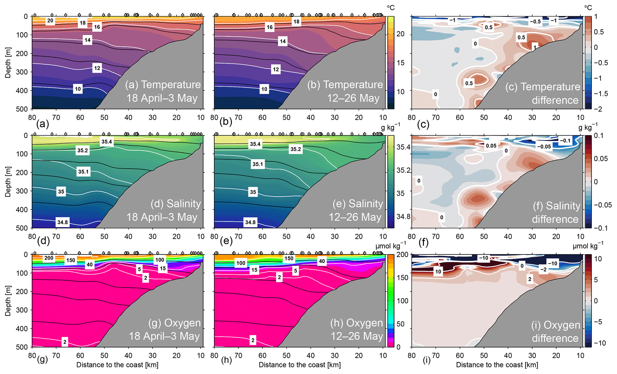
Figure 9 Conservative temperature (a–c), absolute salinity (d–f) and oxygen (g–i) at 12^∘ S during 18 April–3 May 2017 (a, d, g) and 12–26 May 2017 (b, e, h). The difference of the respective characteristic between the two periods is indicated in panels (c), (f) and (i). Black lines indicate the distribution of isopycnals (σ_θ) at 25.6, 25.9, 26.2, 26.4 and 26.7 kg m⁻³. Grey diamonds mark positions of CTD stations.

Distributions of oxygen concentrations were characterized by a sharp oxycline above the anoxic OMZ (Fig. 9g and h). During the weak PCUC period, oxygen concentrations decreased from slightly supersaturated at the surface to anoxia within the upper 100 m of the water column (Fig. 9g). Between 450 and 500 m, oxygen concentrations started to increase again to detectable values (Fig. 9g). When the poleward flow intensified, oxygen levels of waters below about 100 m depth increased (Fig. 9i) and low-oxygen waters were found deeper in the water column than previously (Fig. 9h). Part of the increased oxygen levels were due to the downward displacement of the isopycnals (Fig. 9h), particularly in the near-bottom waters above the continental slope. There, oxygen concentrations larger than 2 µmol kg⁻¹ were observed at 200 m depth in bottom waters (Fig. 9h), a depth range that is usually occupied by anoxic water masses. Such ventilation events have significant consequences for benthic and pelagic biota and for biogeochemical processes in that depth range, as further discussed below.

In the upper water column above 400 m, waters with potential density anomalies larger than 25.9 kg m⁻³ were predominantly ESSW (Fig. 10). ESSW originates from the equatorial current system. It is characterized by a linear relationship of temperature and salinity in the temperature range 8–14 ^∘C and salinity range 34.6–35.0 (e.g. Grados et al., 2018). Lower salinity eastern South Pacific Intermediate Water (temperature range 12–14 ^∘C, salinity 34.8), which is also situated in the depth range mentioned above, was only observed in the hydrographic data from two offshore stations (Fig. 10a). The dominance of ESSW was not affected by the increasing poleward velocities (Fig. 10b) and most profiles followed the same temperature and salinity relationship in both phases. In fact, during PCUC intensification, the ESSW was the sole water mass in the upper 400 m within 80 km of the coast (Fig. 10b).

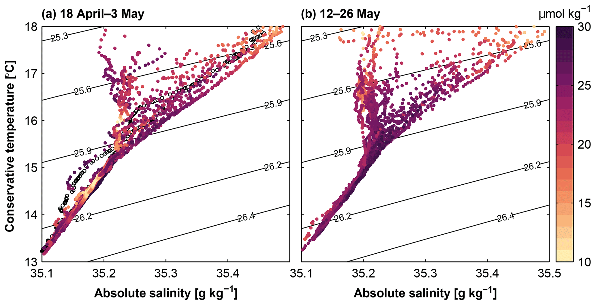
Figure 10 Conservative temperature – absolute salinity diagram between 50 and 300 m depth for CTD profiles between the 100 and 400 m isobaths during 18 April–3 May 2017 (a) and 12–26 May 2017 (b). Colour code depicts nitrate concentrations. Black contours indicate isopycnals (σ_θ) in kg m⁻³.

4.4 Response of nutrient biogeochemistry to PCUC intensification

Nutrients are supplied to the upwelling region by poleward transport within the PCUC. In the following, we relate the observed changes in nutrient concentrations to the PCUC variability and to microbially mediated biogeochemical processes (Sect. 3.2.1). In the anoxic core of the OMZ, denitrification represents a prominent process of anaerobic organic matter degradation and a major sink for reactive nitrogen (Kalvelage et al., 2013; Gruber, 2008). During denitrification, nitrate is stepwise reduced to N₂, with nitrite and nitrous oxide, as important intermediate products. Subsequently, nitrite is either further reduced to N₂ via denitrification or may be used in the microbially driven anaerobic oxidation of ${\mathrm{NH}}_{\mathrm{4}}^{+}$ to N₂ known as annamox (anaerobic ammonium oxidation) (Kuypers et al., 2005; Lam et al., 2009), which leads to a loss of reactive nitrogen. The distributions of nitrate (Fig. 11a and b) and nitrite concentrations (Fig. 11d and e) demonstrate the transformation of nitrate to nitrite. In the open ocean, nitrate increases with depth in the upper 1000 m, whereas on the Peruvian margin a nitrate minimum in the anoxic core of the OMZ is pronounced at 12^∘ S (Fig. 11a and b), co-occurring with a maximum in nitrite.

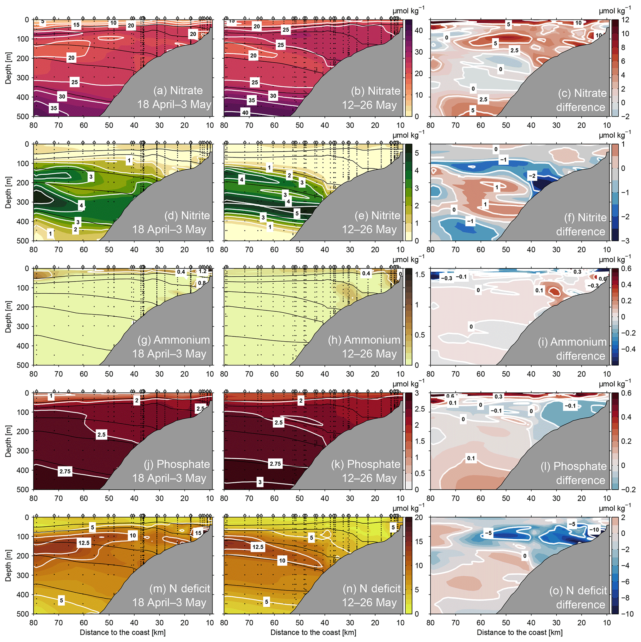
Figure 11 Nitrate (top row), nitrite (second row), ammonium (third row), phosphate (fourth row) concentrations and nitrogen deficit (bottom row) at 12^∘ S during 18 April–3 May 2017 (left panels) and 12–26 May 2017 (middle panels). Concentration difference of the respective parameters between the two time periods are shown in the right panels. Black lines indicate the distribution of isopycnals (σ_θ) at 25.6, 25.9, 26.2, 26.4 and 26.7 kg m⁻³. Grey diamonds mark the positions of CTD stations and black circles mark the position of bottle samples in the water column.

During the period of PCUC intensification, nitrate concentrations on the shelf and upper slope increased (Fig. 11a and b). Before the intensification, nitrate concentrations in the upper 300 m of the water column hardly exceeded 25 µmol kg⁻¹ and particularly low concentrations were found in bottom waters on the shelf, where a local minimum with less than 15 µmol kg⁻¹ is reached (Fig. 11a). As the PCUC intensified, nitrate concentrations between 50 and 250 m mostly exceeded 25 µmol kg⁻¹ (Fig. 11b). Throughout this part of the section, the increase was higher than 2.5 µmol kg⁻¹ (Fig. 11c) and exceeded 5 µmol kg⁻¹ in some areas.

On the other hand, nitrite concentrations in deeper and bottom waters on the shelf and upper slope were reduced during the intensified PCUC period (Fig. 11d and e). In general, nitrite concentrations in oxygenated waters (O₂ >2 µmol kg⁻¹ were less than 1 µmol kg⁻¹, which is likely due to nitrification. In the anoxic core of the OMZ, the nitrite distribution featured two maxima: one in the upper part of the OMZ between 150 and 200 m depth and another in the centre of the OMZ at 300 m depth, both having concentrations of up to 5 µmol kg⁻¹. During the PCUC intensification period, the upper boundary of nitrite containing water was displaced downwards (Fig. 11e) following the displacement of anoxic waters (Fig. 9h). This caused a nitrite decrease exceeding 2 µmol kg⁻¹ in the deeper and bottom water on the continental slope at about 200 m depth (Fig. 11f).

Ammonium concentrations were generally low or undetectable. Concentrations in excess of 0.4 µmol kg⁻¹ occurred only close to the surface on the upper shelf (Fig. 11g and h). It should be noted that in the Peruvian upwelling region, the sediments are a strong source of ammonium (e.g. Sommer et al., 2016). However, despite taking water samples for nutrient analysis very close to the sea floor, elevated ammonium concentrations could not be detected, suggesting a fast removal by annamox of ammonium which was released from the sediments. In the event that oxygen was present, ammonium could also have been nitrified to nitrate.

Phosphate concentrations did not change considerably during the PCUC intensification period (Fig. 11j and k). Concentrations were low at the surface and increased to 2 µmol kg⁻¹ at 50 m depth. Within the upper OMZ, the concentrations were higher offshore than onshore (Fig. 11j and k). When the PCUC intensified, concentrations decreased in approximately the same region in which the nitrate increase occurred (Fig. 11l). A phosphate decrease of up to 0.3 µmol kg⁻¹ occurred in bottom waters on the shelf at water depths shallower than 100 m.

The nitrogen deficit (N_def, Sect. 3.2.1) was reduced during the period of PCUC intensification (Fig. 11m–o). Whilst the PCUC was weak, waters having a nitrogen deficit between 5 and 15 µmol kg⁻¹ were present at depths between 100 and 400 m. Maximum values were found on the continental shelf and offshore between 100 and 200 m (Fig. 11m). During the PCUC intensification period, the nitrogen deficit maximum at the continental shelf disappeared and low-deficit waters (N_def <5 µmol kg⁻¹) occupied the upper 200 m of the water column inshore of 40 km (Fig. 11n). The reduced nitrogen deficit was due increased nitrate concentrations (Fig. 11c) and somewhat reduced phosphate concentrations (Fig. 11l). Furthermore, the region with reduced N_def agrees well with the location of maximum poleward flow during the PCUC intensification period (Fig. 3b). This suggests that poleward advection in the intensified PCUC was the main cause for the observed changes in biogeochemical properties.

5 Summary and discussion

Measurements from an intensive physical and biogeochemical shipboard sampling programme off Peru at 12^∘ S carried out between 7 April and 24 June 2017 are used to analyse intraseasonal variability of the eastern boundary circulation and associated changes in hydrography and nutrient distributions. Our most prominent finding is an intensification of poleward flow within the depth range occupied by the PCUC that started early May 2017 and lasted for about 35 d. During this period, poleward velocities occupied the whole water column above 1000 m depth and extended to more than 80 km offshore. Maximum velocities in the PCUC core between 50 and 100 m depth were above 0.5 m s⁻¹, about 5 times larger than the respective climatological PCUC velocities (Chaigneau et al., 2013) at this latitude.

The elevated poleward velocities were most likely caused by a downwelling CTW. Satellite SLA data indicate a positive anomaly propagating eastward from the eastern equatorial Pacific to the South American coast and subsequently poleward to beyond 14^∘ S. An elevated westerly wind anomaly on the Equator in the central Pacific that occurred in April 2017 is suggested to have excited the initial Kelvin wave. Wind stress and wind stress curl variability along the South American coast did not impact the CTW nor the elevated alongshore velocities. The phase speed of the SLA signal propagation along the South American coast is consistent with a first-vertical-mode CTW. Similarly, the vertical distribution of the poleward velocity anomaly at the eastern boundary generally agreed with the cross-shore-depth velocity structure of a first-mode CTW.

While temperature and salinity conditions remained almost unaltered, the enhanced poleward water mass advection due to the CTW induced changes in the distribution of oxygen and nutrient along the eastern boundary. Below 100 m depth, oxygen concentrations increased and the upper boundary of anoxic water (O₂ >2 µmol kg⁻¹) deepened by about 50 m due to both, the downward displacement of the isopycnals in the thermocline and the advection of ESSW having higher oxygen concentrations. Similarly, nitrate concentrations increased during the period of intensified poleward flow, while phosphate concentrations and nitrogen deficit decreased (Fig. 12).

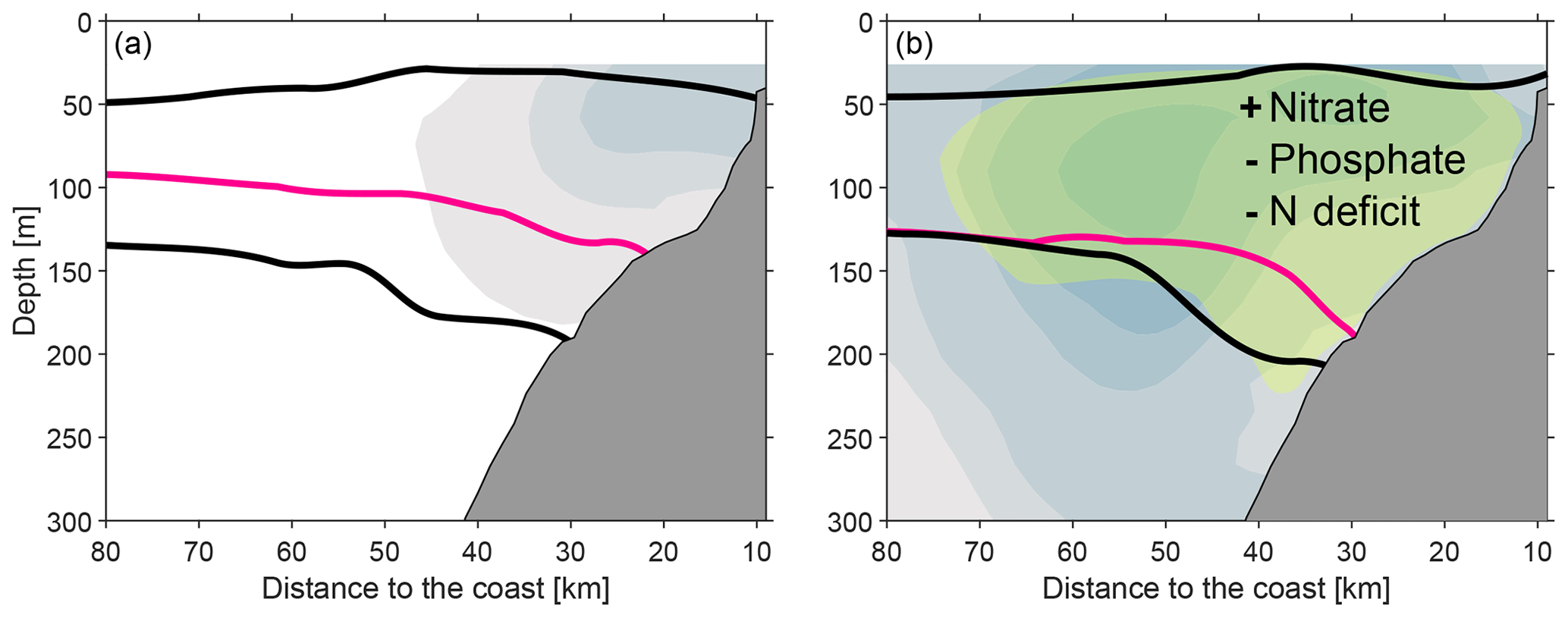
Figure 12 Schematic of the conditions off Peru during the initial phase of weak PCUC flow (a) and strong PCUC flow (b). Alongshore circulation is shown as colour shading, two isopycnals are shown in black, and the top of the anoxic zone is shown in magenta (represented by the 2 µmol kg⁻¹ isoline). The green shaded area in panel (b) shows the region of increased nitrate, decreased phosphate concentrations and decreased nitrogen deficit.

Similar to our results, previous studies have identified the first vertical mode CTWs to dominate intraseasonal variability in the eastern South Pacific based on tide gauge and SLA observations (e.g. Brink, 1982; Shaffer et al., 1997) and model results (Illig et al., 2018b). However, there is disagreement in the details of the observed cross-shore-depth alongshore velocity structure of the CTW and the velocity structure of a first-vertical-mode solution of a linear wave model using local stratification and topography suggesting that additional dynamical processes are important.

A possible explanation of the poor agreement is interaction of the CTW with local topography. North of our sampling site, the continental slope bends offshore at depths between 500 and 1000 m (Fig. 1, insert) while the shelf narrows to the south. Changes in coastline, shelf width and along-slope bathymetry lead to a transfer of CTW energy into higher modes (scattering) and upstream backscattering (Wang, 1980; Wilkin and Chapman, 1990; Kämpf, 2018; Brunner et al., 2019). The influence of changes in shelf width on the upstream alongshore flow structure can extend to 200 km upstream (Wilkin and Chapman, 1990) but, due to relative smooth downstream topography, is likely not relevant here. However, the bend of the continental slope and other topographic irregularities north of our sampling site may stimulate energy transfer into high-vertical-mode CTWs. In turn, the superposition of several vertical modes could explain the observed elevated poleward flow between 50 and 300 m depth (Figs. 3 and 12) that cannot be explained by a first-mode CTW. In fact, a recent model study suggests that differences between the theoretical CTW solutions and observations are predominately due to wave scattering (Brunner et al., 2019).

The temperature and salinity conditions on the shelf remain almost unchanged despite the strongly intensified poleward flow, suggesting that the same water mass was advected within the boundary current regime during both observational periods. However, during the presence of the CTW, SSTs were lower than in the period prior to the wave. This is a somewhat unexpected result because downwelling CTWs weaken coastal upwelling due to the downward displacement of the thermocline which should lead to warmer SSTs and earlier in March 2017 downwelling CTWs contributed to the anomalously high SST in the coastal El Niño (Echevin et al., 2018; Peng et al., 2019). However, previous studies have shown that the impact of CTWs on intraseasonal SST variability off Peru is limited (Dewitte et al., 2011; Illig et al., 2014). Specifically, in May 2017 SST reduction agrees with both the seasonal cycle (Graco et al., 2017) and the decline of the warm Coastal El Niño with peak SST in March (e.g. Garreaud, 2018).

Changes in oxygen concentrations due to the CTW event were rather small. In the water column between 100 and 200 m depth, oxygen concentrations increased by 1 to 10 µmol kg⁻¹, only. However, the limited impact of the CTW on the oxygen distribution is likely related to high oxygen concentrations present at the study site before the wave passage. Previous measurement programmes in this area found the mean depth of the upper boundary of the OMZ on the shelf at about 50 m depth (Gutiérrez et al., 2008; Dale et al., 2015; Graco et al., 2017) but deepening to 200 m or more during El Niño–Southern Oscillation (ENSO) years (e.g. Levin et al., 2002; Espinoza-Morriberón et al., 2019). In particular, Dale et al. (2015) found oxygen levels below the detection limit between 30 and 400 m depth during previous measurement programmes along 12^∘ S. It is thus likely that the prevailing elevated oxygen concentrations are related to the coastal El Niño event in the same way that canonical El Niño events are related to enhanced oxygenation (Helly and Levin, 2004; Espinoza-Morriberón et al., 2019). Despite small oxygen concentration changes, the upper boundary of anoxic water deepened by about 50 m during the presence of the CTW (Fig. 12). The change from anoxic conditions to suboxic conditions with oxygen concentrations (O₂ >2 µmol kg⁻¹) has important consequences for biogeochemical processes and the benthic and pelagic communities (e.g. Gutiérrez et al., 2008). This study thus confirms previous suggestions that CTW led to episodic oxygenation events that are vital for colonization of invertebrates and other biotas within the predominately anoxic regions of the benthos and the water column above.

The increase in nitrate concentrations and the reduced nitrogen deficit are likely caused by the faster advection during the intensified flow period. The nitrate concentrations in the ESSW increase and waters with the same temperature–salinity properties are richer in nitrate following the intensification of the PCUC (Fig. 10), indicating the nitrate increase was not due to a different source of advected water. Along the ESSW pathway within the PCUC from the Equator to 12^∘ S, the nitrogen deficit increases while nitrate concentrations decrease (Silva et al., 2009; Zamora et al., 2012; Kalvelage et al., 2013). The resulting nitrogen deficit accumulates with time during the poleward advection. Thus, an intensified PCUC increases the poleward advection of water with a lower nitrogen deficit. This can be verified by investigating the advection timescales. The alongshore distance from the Equator to the 12^∘ S (1800 km) and a PCUC velocity of 0.4 m s⁻¹ yields a timescale of 52 d, while a timescale of 160 d results from a velocity of 0.13 m s⁻¹ representing maximum climatological velocity (Chaigneau et al., 2013). Using a rate for N loss of 48 nmol N L⁻¹ d⁻¹ (combined anammox and denitrification rates in the coastal OMZ from Kalvelage et al., 2013) results in an N-loss difference of 5.2 µmol N L⁻¹ due to the lower flow velocities. Indeed, the reduction of the nitrogen deficit by about 5 µmol N kg⁻¹, as observed throughout much of the PCUC core during the presence of the CTW, closely relates to this estimate. The sediments off Peru subjected to oxygen-depleted bottom waters release phosphate into the water column (Noffke et al., 2012; Lomnitz et al., 2016) that also contributes to the nitrogen deficit. Faster advection leads to a reduced accumulation of phosphate that is released from the sediments with lower phosphate concentrations during the strong PCUC flow. However, the increase of nitrate exceeds the phosphate decrease by about 5 to 0.1 µmol kg⁻¹, a ratio higher than the nitrogen-to-phosphorus ratio given in Eq. (1). Therefore, changes of nitrate concentration dominate the reduction of the nitrogen deficit.

The increase in nitrate by the downwelling CTW implies that the change in alongshore advection with the increased flow is more important for the nitrate balance than downwelling. The downwelling would displace the nutricline and thus transfer low-nutrient surface waters downwards, lowering nutrient concentrations, which was not observed. The decline in nitrate concentrations during El Niño events has been associated with a nutricline displacement due to downwelling CTWs on interannual timescales (Graco et al., 2017; Espinoza-Morriberón et al., 2017). However, focusing on intraseasonal timescales, Echevin et al. (2014) modelled an almost cancelling of horizontal and vertical (i.e. nutricline movement) advection and a fast-mode CTW not impacting nutricline depth. In a model study in the Atlantic Ocean, where nitrate decreases poleward as well, it was shown that the total effect of CTWs on nitrate concentrations varies regionally due to a different balance of horizontal and vertical advection, but the horizontal advection always led to an increase in nitrate (Bachèlery et al., 2016).

The changes in redox state in the water column and especially bottom waters affect the biogeochemical cycling in the sediment as well. Because microbial storage of nitrate and nitrite by microorganisms in the sediment can sustain vigorous N turnover even in the absence of bottom water nitrate and nitrite (Dale et al., 2016; Sommer et al., 2016), episodic events of nitrogen supply can be associated with continuous benthic nitrogen cycling. The absence of nitrate supply due to the absence of CTWs over longer time periods favours the depletion of nitrate in the water column as observed by Sommer et al. (2016) and may lead ultimately to the development of sulfidic events (Schunck et al., 2013; Dale et al., 2016; Callbeck et al., 2018).

6 Conclusions

Based on extensive physical and biogeochemical sampling, we describe and analyse the evolution of circulation, hydrography and biogeochemistry off Peru in 2017. Poleward velocities within the PCUC intensified in May 2017 to several times the reported climatological mean. This increased flow occurs during a limited time period in May in between weaker poleward transport in April and late June. The propagation velocity of positive SLA along the Equator and coastline suggests that the intensified current is caused by a poleward propagating downwelling CTW of the first baroclinic mode forced around 160^∘ W at the Equator that caused a positive SLA signal east of 95^∘ W. The transition of the circulation from a weak poleward flow to strong poleward flow decreased the timescale of alongshore advection from the equatorial current regime to the study site at 12^∘ S.

The downwelling CTW is not associated with strong vertical displacements of waters; instead, the advection caused by the intensified PCUC is more important. For parameters without strong horizontal gradients, an increase in PCUC flow does not cause pronounced changes in the advection. In this study, this applied to the conservative properties of temperature and salinity as well as for oxygen where alongshore gradients are weak (Zamora et al., 2012). For these parameters, there are no large differences between both circulation phases that can be attributed clearly to the altered circulation. Yet concentrations of nutrients are influenced by shorter transit times, being less altered by biogeochemical cycling. This leads to an increase of bioavailable nitrogen in the OMZ (Fig. 12) and its biogeochemistry is strongly changed by the increased ratio of nitrogen to phosphorus related to the increased advection.

For the period from April to May 2017, our study suggests an increase in nitrate levels due to the passage of an intraseasonal downwelling CTW. This contrasts with the decrease observed previously on interannual timescales caused by downwelling CTWs (Graco et al., 2017). This shows that the impact of CTWs on nutrient biogeochemistry is a complex balance between different factors, with potentially different outcome on different timescales. Analysing the processes associated with individual intraseasonal waves is also necessary to understand the interannual effect of CTWs, which is based on varying occurrence of such waves in different years.

The high variability of circulation, nutrients and the nitrogen deficit demonstrates the need for temporally resolved sampling as an individual section recorded may be very different from the situation a few weeks later. Quantification of intraseasonal variability in CTWs and their impact is – other than in modelling studies (e.g. Echevin et al., 2014) – only possible by sampling at high temporal resolution.