Assimilation of chlorophyll data into a stochastic ensemble simulation for the North Atlantic Ocean

Satellite-derived surface chlorophyll data are assimilated daily into a three-dimensional 24-member ensemble configuration of an online-coupled NEMO (Nucleus for European Modeling of the Ocean)–PISCES (Pelagic Interaction Scheme of Carbon and Ecosystem Studies) model for the North Atlantic Ocean. A 1-year multivariate assimilation experiment is performed to evaluate the impacts on analyses and forecast ensembles. Our results demonstrate that the integration of data improves surface analysis and forecast chlorophyll representation in a major part of the model domain, where the assimilated simulation outperforms the probabilistic skills of a non-assimilated analogous simulation. However, improvements are dependent on the reliability of the prior free ensemble. A regional diagnosis shows that surface chlorophyll is overestimated in the northern limit of the subtropical North Atlantic, where the prior ensemble spread does not cover the observation's variability. There, the system cannot deal with corrections that alter the equilibrium between the observed and unobserved state variables producing instabilities that propagate into the forecast. To alleviate these inconsistencies, a 1-month sensitivity experiment in which the assimilation process is only applied to model fluctuations is performed. Results suggest the use of this methodology may decrease the effect of corrections on the correlations between state vectors. Overall, the experiments presented here evidence the need of refining the description of model's uncertainties according to the biogeochemical characteristics of each oceanic region.

1 Introduction

Estimating the biogeochemical state of the ocean has become fundamental under the current climate change context due to its key role in mediating global carbon stocks (e.g., Houghton et al., 2001). Currently, the optimal combination of observational data with the dynamical equations embedded in models through data assimilation (DA) is the most comprehensive strategy to meet this goal. Therefore, there is a growing effort towards the development of effective DA techniques to improve hindcasts, forecasts, nowcasts, and scenario simulations of ocean biogeochemistry (e.g., Brasseur et al., 2009; Yu et al., 2018; Fennel et al., 2019). At present, the Copernicus Marine Environment Monitoring Service (CMEMS) delivers DA biogeochemical products only for selected regions (von Schuckmann et al., 2019), though the operational production of the data-assimilated biogeochemical state of the ocean is one of its challenging core objectives.

In order to achieve model–data integration it is of utmost importance to explicitly identify the structure of the uncertainties that affect the model and the observations (Lahoz et al., 2010). In this sense, ensemble methods (e.g., Bessières et al., 2017) are designed to provide a statistical description of the inaccuracies associated with a complex model system by describing the evolution of the probability density function (PDF). An appropriate approach to perform ensemble simulations is by introducing stochastic noise into the (deterministic) model equations to simulate the effect of the uncertainties. Stochastic parameterizations have been used in meteorological forecasting (e.g., Buizza et al., 1999; Leutbecher et al., 2017) and are becoming the standard procedure for climate modeling (see Palmer, 2012; Berner et al., 2017). In oceanography, the implementation of this type of probabilistic approach has increased in the last decade (e.g., Brankart et al., 2015; Juricke et al., 2017), although its application in physical–biogeochemical models is quite unusual.

In a precursory study, stochastic perturbations were applied to a deterministic solution of the Mercator Ocean (http://www.mercator-ocean.fr., last access: December 2019) North Atlantic 0.25^∘ configuration of the NEMO (Nucleus for European Modeling of the Ocean)–PISCES (Pelagic Interaction Scheme of Carbon and Ecosystem Studies) coupled model to parameterize selected model uncertainties associated with some poorly resolved processes (see Garnier et al., 2016, for more details). Ensemble simulations involving 60 members were performed using a probabilistic version of the NEMO-PISCES simulation for the year 2005. An objective diagnosis of this ensemble simulation showed its probability distribution is quite consistent with ocean color observations in the most productive regions of the North Atlantic, a prerequisite to undertake DA applications.

Ocean color data have been successfully used in DA procedures for improving the simulation of nutrients and primary production in ocean models (e.g., Gregg, 2008; Ciavatta et al., 2011; Ford et al., 2012; Fontana et al., 2013; Teruzzi et al., 2018). However, none of the latter studies explicitly incorporate the uncertainties in the ocean biogeochemistry introduced by stochastic approaches on the model formulation. In this context, the overarching aim of the present work is to investigate to what extent the parameterizations developed in Garnier et al. (2016) can be implemented to build a complete 4D assimilation system using ocean color data that will update the state-of-the-art of biogeochemical DA. Our strategy will rely on the daily integration of surface chlorophyll (Chl a hereafter) data within the latter probabilistic solution. To that end, 24 trajectories of the original ensemble are daily updated by a square root algorithm based on the SEEK (singular evolutive extended Kalman) filter (Pham et al., 1998; Brasseur and Verron, 2006) using daily composites of ocean color observations extracted from MERIS (MEdium Resolution Imaging Spectrometer). Following this strategy, a 1-year experiment is performed in order to investigate the effects of the assimilation in contrasted periods (e.g., bloom vs. nutrient-depleted periods) throughout the annual cycle.

The paper is structured as follows. Sect. 2 presents the coupled model, the assimilation scheme, and the validation metrics. Section 3 presents the results of the experiment and provides a probabilistic assessment as compared with a non-assimilated ensemble simulation. A discussion of the most relevant outputs is carried out in Sect. 4. In particular, we assess how the DA system based on parameterized uncertainties can reduce the model uncertainties, and we evaluate its performance in selected regions. Lastly, a summary, conclusions, and future perspectives are given in Sect. 5, in which we suggest directions for the next possible developments.

2 Material and methods

2.1 Hydrodynamical model

The assimilation system presented here is based on a realistic three-dimensional physical–biogeochemical simulation. The physical component is simulated using the primitive equation free-surface ocean circulation model NEMO (version 3.4; Barnier et al., 2006; Madec et al., 2015), whose prognostic variables are temperature, salinity, and the three-dimensional velocity fields.

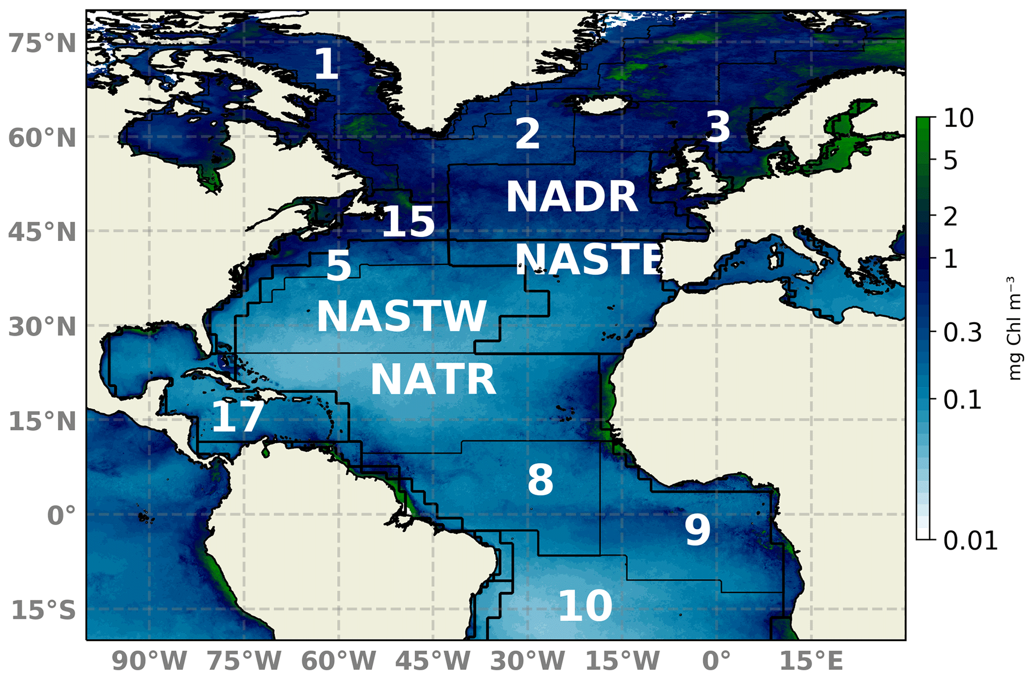
Figure 1 Schematic map of the North Atlantic basin showing the NATL-025/PISCES domain. Longhurst et al. (1995) biogeochemical provinces are indicated. Provinces are indicated by abbreviations: NADR (North Atlantic Drift), NATR (North Atlantic tropical gyre), NASTE (northeast Atlantic subtropical gyre), and NASTW (northwest Atlantic subtropical gyre) are used throughout the text. A 2018 yearly composite of sea surface Chl a is superimposed.

The model configuration is a duplicate of the North Atlantic configuration developed within the framework of the project DRAKKAR (referred to here as NATL025; Barnier et al., 2006, https://www.drakkar-ocean.eu, last access: October 2017), which covers the North Atlantic region from 20^∘ S to 80^∘ N and 98^∘ W to 23^∘ E (Fig. 1). The numerical grid has a horizontal resolution of 0.25^∘ and 46 geopotential levels in the vertical from surface to 6000 m depth. Such an eddy-permitting resolution enables a rough representation of mesoscales features, which are key elements for primary production (Oschlies and Garçon, 1998; Lévy et al., 2012). The dynamical component is forced by ERA-INTERIM atmospheric fields (Simmons, 2006; Dee et al., 2011). This configuration has already been coupled to biogeochemistry modules and evaluated in recent numerical studies (e.g., Ourmières et al., 2009; Doron et al., 2011, 2013; Fontana et al., 2013; Garnier et al., 2016).

2.2 Biogeochemical model

The biogeochemical component coupled to hydrodynamics is PISCES (version 2; Aumont et al., 2015). PISCES is a complex carbon-based model that simulates marine biological productivity and carbon biomass based upon five main nutrients: nitrate, ammonium, phosphate, silicate, and iron. Its architecture includes 24 biogeochemical variables grouped into four main compartments: nutrients, phytoplankton, zooplankton, and detritus. PISCES has been used in global simulations (e.g., Bopp et al., 2015), environmental studies (e.g., Brasseur et al., 2009), climate studies (Lefort et al., 2015), basin-scale studies (e.g., Jose et al., 2014), and, more recently, in regional-scale studies (e.g., Auger et al., 2015). For more details, see Aumont et al. (2015) where a complete description of PISCES equations along with a brief validation are presented.

PISCES differentiates between two phytoplankton functional types: diatoms and nanophytoplankton. The parameterization of diatoms differs from nanophytoplankton in their requirements of silicate (Si), an increased consumption of iron (Fe), and a higher level of nutrient saturation due to their larger size. Both Chl a content on nanophytoplankton and diatoms is parameterized using the photo-adaptative model of Geider et al. (1997). Here we ascribe Chl a as the direct sum of these two compartments, and it will be used as a proxy for primary production. Besides biomass of Chl a, carbon ratios with Fe and Si (only for diatoms) are explicit prognostic variables of the model. Furthermore, PISCES discretizes two sizes of zooplankton (micro- and mesozooplankton) and three classes of nonliving compartments: the semi-labile dissolved organic carbon pool and two sizes of particulate organic carbon that differ by their sinking velocities (3 m d⁻¹ for small particles and 50 to 200 m d⁻¹ for large particles).

PISCES is coupled online to NEMO with a coupling frequency equal to the circulation model time step (i.e., 40 min). Note that online coupling is a one-way forcing of the ecosystem model by the circulation model, since no feedback of the ecosystem model is taken into account. This strategy of online coupling with a maximum frequency is thought to be useful for simulating the ecosystem evolution, while avoiding possible problems brought by the use of averaged physical fields, as in off-line coupling.

A realistic dynamical adjustment of the modeled ocean state is obtained after a 13 years of spin-up (1989–2002) starting from the Levitus climatology for temperature and salinity (Levitus et al., 1998). After physical spin-up, the biogeochemical component is initialized in January 2002 from outputs of a global 0.25^∘ PISCES operational simulation performed by MERCATOR Ocean (Elmoussaoui et al., 2011). Between January 2002 and December 2004, a 3-year spin-up is performed to ensure a consistent biological initial state. After this period, a deterministic simulation of the coupled system, i.e., NATL025-PISCES, is performed for a period of 6 years, extending from January 2005 to December 2010. This simulation is used to build a probabilistic configuration upon which a data assimilation system is performed.

2.3 Probabilistic version of the coupled system

Any realistic description of the state of a system involves uncertainties. In the case of coupled ocean models, uncertainties may originate from external forcings (e.g., the atmospheric data), parameterizations of physical and biological processes that are not explicitly resolved by the model, omission of unresolved scales, and reduced complexity to limit computational costs. In a previous study (Garnier et al., 2016), two classes of these uncertainties were parameterized to explicitly simulate the errors associated with the deterministic model formulation: (1) the limitations of the spatial scales resolved by the model and (2) the simplification of the description of the biogeochemical system to a limited number of state variables and parameters. The first were described by following the approach proposed in Brankart et al. (2015), and the second was simulated by introducing lognormal stochastic perturbations on seven key biogeochemical parameters whose uncertainties may have a direct impact on the estimation of primary production. Specifically, the parameters perturbed are the phytoplankton growth rate at 0 ^∘C, the initial P-I slope for both nanophytoplankton and diatoms, the phytoplankton temperature sensitive to growth, the zooplankton temperature sensitive to grazing, and the growth dependency on the length of day for both nanophytoplankton and diatoms. For the perturbations, the starting point is a first-order autoregressive process setting up with a standard deviation of 0.3 and a decorrelation timescale of 1 month, at which a random noise is drawn at each grid point and at each time step. After spatial filtering, Gaussian noises are transformed in lognormal noises to guarantee positivity. Stochastic perturbations are then introduced by multiplying by these lognormal noises. To preserve vertical consistency, all perturbations are set as identical for the whole water column. In addition, as the effects of unresolved scales will have an impact on the large-scale biogeochemical representation, we create a perturbation that simulates the unresolved fluctuation of the concentration of each parameter within every model grid box.

The stochastic formulation was introduced to produce an ensemble spread that is large enough for building a DA system while keeping the coupled model stable. A 60-member ensemble simulation for the year 2005 was performed by Garnier et al. (2016), who show that the resulting probability distribution (of the annual ensemble simulation) is quite consistent with SeaWiFS (Sea-viewing Wide Field-of-View Sensor) ocean color observations. Specifically, they assessed the reliability or statistical consistency of the ensemble simulation by comparing it with satellite Chl a data assuming 30 % of observation error.

The present study is based on these previous developments, with some additional adjustments to prepare for DA. In particular, we carried out sensitivity experiments to select an ensemble size that is more cost-efficient but with the same level of agreement to observations as in Garnier et al. (2016). More explicitly, 1-month assimilation experiments were performed by reducing the ensemble size from the original 60 members to 12 and 24 members. We first compared each of them with the original experiment, and observed surface Chl a differences below 0.5 mg Chl m⁻³ for most regions between the 24 and the 60-member ensembles. A comparison with the observations used for the assimilation process was also assessed. Both reduced ensemble simulations were able to reproduce the main patterns of surface Chl a displayed by satellite observations. However, global probabilistic metrics showed that only the 24-member ensemble experiment conserves the same level of statistical consistency as the original ensemble, while reducing computational costs of the forecast step by up to 60 %. The probability distribution of the 12-member ensemble showed an under-dispersed distribution, while the 24-member ensemble showed the ensemble spread covers a major part of the observations. Therefore, a total of 24 trajectories of the inherited stochastic simulation developed by Garnier et al. (2016) are used here as the prior PDF for the assimilation problem.

2.4 Assimilation scheme

The assimilation system integrates daily composites of MERIS Chl a observations to daily update the ensemble forecast. The methodology behind this process is based on a SEEK filter (Pham et al., 1998; Brasseur and Verron, 2006), implemented in the ensemble system using the System of Sequential Assimilation Modules (SESAM) assimilation platform (Brankart et al., 2012) that deals with all matrix operations required by the assimilation scheme. Though using a probabilistic approach is more resource-intensive, it produces a probability distribution that allows for an objective validation with observations using probabilistic scores, unlike a deterministic assimilation system that provides only one estimated trajectory. As another advantage, the explicit simulation of model uncertainties in the ensemble approach is necessary to produce a description of uncertainties that is consistent with observations.

The assimilation scheme proceeds in two steps. (1) An ensemble forecast in which each ensemble member, i.e., state vector, is propagated forward in time using the full model equations. (2) When a set of observations, i.e., daily swaths of ocean color retrieved from MERIS, is available, the statistical information contained in the ensemble is combined with observations to update the forecasted ensemble. The most relevant aspects of this second step, referred to as analysis, will be commented on below. To propagate the system, the initial condition of the subsequent daily forecast is the updated analysis ensemble obtained by the assimilation of Chl a observations.

The state vector entering the analysis step is composed of all prognostic biogeochemical state variables of the three-dimensional grid following a multivariate approach. To keep the analysis computationally affordable, a prior diagnosis of the multivariate correlations between the observed (Chl a in this case) and non-observed biogeochemical variables has been carried out. Following the results obtained from this test, 12 out of the 24 biogeochemical state variables are included into the updated state vector. These state variables correspond to nutrients, oxygen, zooplankton, phytoplankton, and Chl a.

The probability distribution of the observed variable, i.e., Chl a, is usually regarded as lognormal (Campbell, 1995). A well-known strategy to accommodate the characteristic non-Gaussian distributions of biogeochemical parameters is applying a lognormal transformation (e.g., Ciavatta et al., 2011; Mattern et al., 2017). However, this transformation assumes that the shape of the probability distribution does not change. As this is not often verified, we adopted here another nonlinear strategy dependent on the shape of the probability distribution. Anamorphosis transformations (Bertino et al., 2003; Béal et al., 2010) are applied to each variable of the state vector prior to the ensemble analysis step to ensure that marginal PDFs are close to Gaussian. The strategy of these transformations relies on remapping the quantiles of each marginal distribution such that the probability distribution is as close as possible to a Gaussian. These transformations ensure that no value of the variables becomes negative after the analysis update, improve the description of the correlations between Chl a and non-observed variables, and exclude possible causes of the breakdown of the simulation. To be compliant with the new variables, observations are also transformed into the anamorphic space defined by the ensemble simulation. After analysis, the corresponding inverse transformations are performed to come back into the original model space and initialize the subsequent daily ensemble forecast.

Relatively small ensembles like the one used here can lead to spurious correlations between distant model grid points. In order to avoid the potential negative effects of these correlations, we employ a domain localization methodology in which a separate analysis for each local domain is applied. In practice, this means that an analysis update is performed for each horizontal grid point but including all vertical levels and state variables. To ensure continuity between analyses, each analysis uses the observations within a certain localization radius (of 1^∘ in the present case), with an observation error that increases with distance.

2.5 Assimilated and independent observations

The observational data set assimilated by our system corresponds to daily swaths of ocean color retrieved from MERIS. Specifically, we use Level-3 binned data accessible at http://earth.esa.int/level3/meris-level3/, last access: October 2017, which consist of daily accumulated Level-2 products with a standard bin size of 4.6 km. Among other properties, this product provides Chl a estimations (in mg Chl m⁻³) used here to update the ensemble simulation. Additionally, the system performance will be assessed by comparison with ocean color SeaWiFS data accessible through https://oceancolor.gsfc.nasa.gov/data/seawifs/, last access: December 2019 and with daily surface Chl a fields obtained from the Global Ocean Satellite Observations provided by Copernicus-GlobColour service and accessible through http://marine.copernicus.eu, last access: December 2019. This latter product is based on the merging of several sensors (data from SeaWiFS, MODIS-Aqua, and MERIS sensors are used for the year 2005) delivered at 4 km of spatial resolution.

The limited accuracy of ocean color products is taken into account in the assimilation process. Imperfections in the retrieval process of the Chl a concentrations may be due to the presence of chromophoric dissolved organic matter, atmospheric aerosols, or errors in the algorithms at some specific regions, among others (e.g., Gregg and Casey, 2004; Le Fouest et al., 2006). Therefore, 30 % of observational error is considered in agreement with global average standard deviation estimates (e.g., Gregg and Casey, 2004; Mélin et al., 2016).

While intercomparisons between the data-assimilated simulation and the assimilated observations are necessary to assess the experiment efficiency, the validation strategy is not totally conclusive since they are not independent (Gregg et al., 2009). We thus use an additional independent data set for an objective validation of the assimilation process. Specifically, we use biogeochemical fields extracted from the World Ocean Atlas 2018 (WOA2018; Garcia et al., 2019). The historical in situ nutrient measurements available in this data set were produced by the NOAA's (National Oceanic and Atmospheric Administration) National Oceanographic Data Center – Ocean Climate Laboratory as part of the World Ocean Database project (WOD; Boyer et al., 2013). They will be used to assess the simulation performance on matching the non-observed variables patterns.

2.6 Probabilistic validation

Unlike for deterministic simulations, the validation of our DA experiment requires many realizations (members) to be properly evaluated given its probabilistic nature. For that purpose, reliability and resolution scores (see Toth et al., 2003; Candille et al., 2015, for more information) will be computed from the ensemble. Reliability evaluates the capacity of a model to produce an ensemble probability distribution in agreement with the statistical distribution of a given observation data set. Resolution measures the ability of a model to discriminate distinct observed situations. In other words, the reliability provides information on the system's ability to produce PDFs that agree with a given observation's PDF, while resolution provides information on the spread of the system's PDFs. These metrics will allow us to measure the skills of our ensemble simulation for predicting the true state of the ocean biogeochemistry.

To evaluate reliability and resolution, several probabilistic metrics will be employed. We first check the reliability of the DA system by introducing the rank histogram (Anderson, 1996). Rank histograms are computed by sorting all 24 members in ascending order (in the present case according to their Chl a concentration) for each grid point and at a given date. Each observation is then ranked relatively to its location within this sorted ensemble. Observations smaller than the minimum of the ensemble will take rank “0”, while those observations higher than the maximum of the ensemble will take rank “n”. The statistical consistency of the ensemble can then be evaluated by studying its shape (Candille et al., 2015; Germineaud et al., 2019). Rank histograms may be (1) flat, which indicates the distribution of the model accords accurately with the observations, i.e., perfect reliability; (2) under-dispersed or U-shaped, which indicates the spread of the ensemble is too small (too many observations lie outside the extremes of the ensemble); or (3) over-dispersed or dome-shaped, which indicates the spread of the ensemble is too large (too many observations lie near the center of the ensemble).

To measure the resolution of the system and obtain a full probabilistic validation of the ensemble, we use the continuous rank probability score (CRPS). Let x to be a parameter of interest (Chl a in our case) to which a real observation corresponds. Then CRPS corresponds to the distance between the simulation and the observation, as defined in

$$\text{CRPS}=E\left[\underset{\mathbb{R}}{\int }\right(F_{\mathrm{p}}\left(x\right)-F_{\mathrm{o}}\left(x\right){)}^{\mathrm{2}}\mathrm{d}x],$$

where E is the mean over all observations at a given date, and F_p(x) and F_o(x), the cumulative distributions of the model and the observations.

CRPS can be decomposed as the sum of the ensemble reliability (Reli) and the ensemble potential resolution (Resol), i.e., the resolution in the case of perfect reliability (see Hersbach, 2000, for more details).

$$\text{CRPS}=\text{Reli}+\text{Resol}$$

According to CRPS, a skillful probabilistic system must satisfy two criteria: Reli should be null, and Resol must tend to zero and, in any case, be much inferior to the reference value of the CRPS when it is only based on the reference data set (without data assimilation).

3 Results

It is instructive to evaluate how the assimilation process affects the original ensemble simulation. In this section, the impacts of the assimilation on the variability in space and time of key biogeochemical parameters are assessed by comparing the assimilated experiment with an analogous 24-member ensemble of model simulations in which no observational data have been assimilated. This ensemble run is performed over the same period, and referred to as the “free run”.

3.1 Skill in reproducing surface Chl a

Both the assimilated and the free-run simulations are compared to daily surface Chl a fields obtained from the Global Ocean Satellite Observations (see Sect. 2.5). Merged satellite products are selected here to minimize missing data due to cloud cover and still resolve mesoscale spatiotemporal variability. For the assimilated simulation, the analysis step, which corresponds to the ensemble computed after the update, is shown. Surface Chl a daily composites are presented for three different dates: 19 April, 15 May, and 5 October 2005 (Fig. 2). These dates are selected for representing contrasting periods. The first two dates coincide roughly with the well-documented spring bloom period of the North Atlantic. The availability of light and nutrients during this period drives phytoplankton growth, which leads to relatively high values of Chl a at surface. The last date represents a period after summer when conditions change due to the reduction in sunlight over the surface.

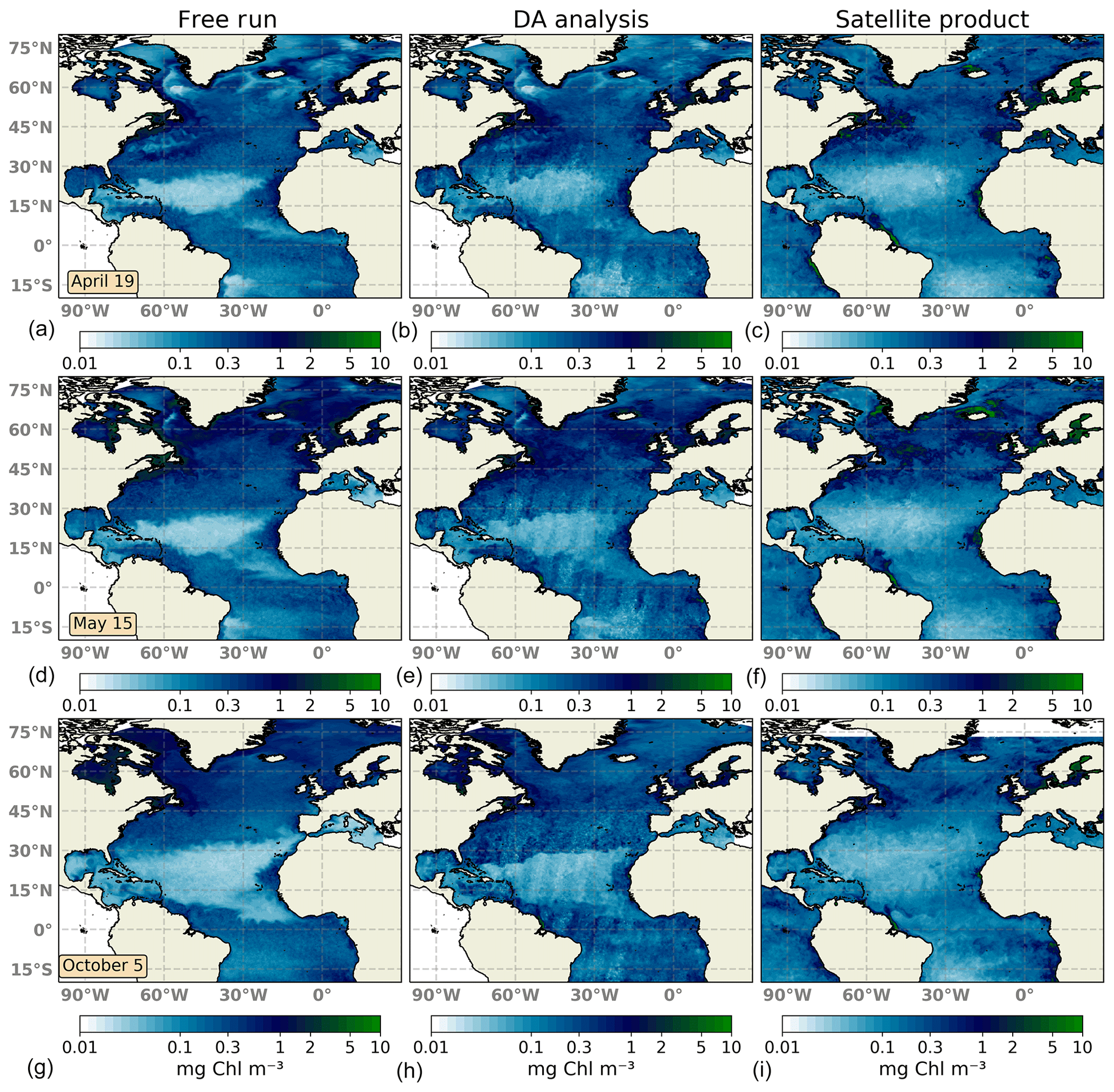
Figure 2 Surface maps of Chl a (mg Chl m⁻³) for 19 April 2005 (a, b, c), 15 May 2005 (d, e, f), and 5 October 2005 (g, h, i). The ensemble median of the non-assimilated free-run experiment (a, d, g), the analysis ensemble median of the assimilation experiment (b, e, h), and merging daily surface Chl a fields obtained from the Global Ocean Satellite Observations (c, f, i) are represented.

The large-scale spatial distribution of surface Chl a is captured by the DA simulation. High Chl a values in regions such as the Gulf Stream, the North Sea, the Amazonian delta, and the western coast of Africa are successfully reproduced during the first days of the experiment (Fig. 2a–c). However, there is too strong a gradient between the oligotrophic conditions of the North Atlantic subtropical gyre and temperate waters to the north. The ensemble median of the free-run experiment displays a stronger gradient, indicating that the assimilation of surface Chl a data slightly improves this situation.

About a month later (Fig. 2d–f), the inferred large-scale picture of surface Chl a distribution remains close to that displayed by satellite observations. The bloom of Chl a in temperate waters is well reproduced by the DA simulation both attending to magnitude and geographical location. Upwelling areas along with other zones with high Chl a concentrations are also well depicted showing a good performance to match highly productive regions. By contrast, the gradient northwards of the oligotrophic open ocean is too pronounced, showing no transition between both regimes as evidenced in the satellite map. Moreover, corrections made by daily satellite swaths leave imprints of their trajectory in the analysis map. These imprints are caused by using a small localization radius. This radius needs to be small due to the small correlation length scale of forecast uncertainties in the Chl a field. Thus, the impact of a given observation on the update remains local. They should disappear over time as the magnitude of the innovation decreases. In this experiment, however, the time lag between observations is quite large with respect (5 to 7 d) to the typical timescale of the system. For its part, the free run overestimates Chl a in high-latitude regions, while it underestimates it within the North Atlantic subtropical gyre.

After the summer period, at the beginning of October 2005 (Fig. 2g–i), the Chl a distribution changes; regions with the highest concentrations relaxed their values, while concentrations in the open ocean slightly increased. The representation of surface Chl a degrades during this period. Concentrations within the subtropical gyre agree with observations, but gradients both at its northern and southern boundaries are too strong. In this transition zone, inferred values double the concentrations displayed by observations. In the rest of the domain, the Chl a pattern improves that shown by the non-assimilated simulation. The free-run experiment exhibits a strong overestimation in the Gulf Stream region as already observed by Garnier et al. (2016) with a 60-member non-assimilated version of the coupled model. Moreover, oligotrophic conditions at the subtropical gyre are too low, which may indicate the spread of the ensemble is unable to capture the whole observation's variability.

3.2 Probabilistic regional assessment

An ensemble system should be statistically consistent with observations in order to be objectively regarded as realistic. To evaluate the reliability metric, we present rank histograms (Fig. 3) computed for each grid point by accumulation over all 24 members of the ensemble at four different Longhurst provinces (Longhurst et al., 1995; Fig. 1 provides the location of the provinces). The provinces used are NADR (North Atlantic Drift), NATR (North Atlantic tropical gyre), NASTE (northeast Atlantic subtropical gyre), and NASTW (northwest Atlantic subtropical gyre). Both the assimilation analysis and free-run ensembles are displayed. Ranks are computed against SeaWiFS ocean color data extracted for the same day with a specified 30 % of observation error. In practice, the latter error means that for each realization a Gaussian white noise with a standard deviation of 30 % of the satellite Chl a concentration is added to each ensemble member.

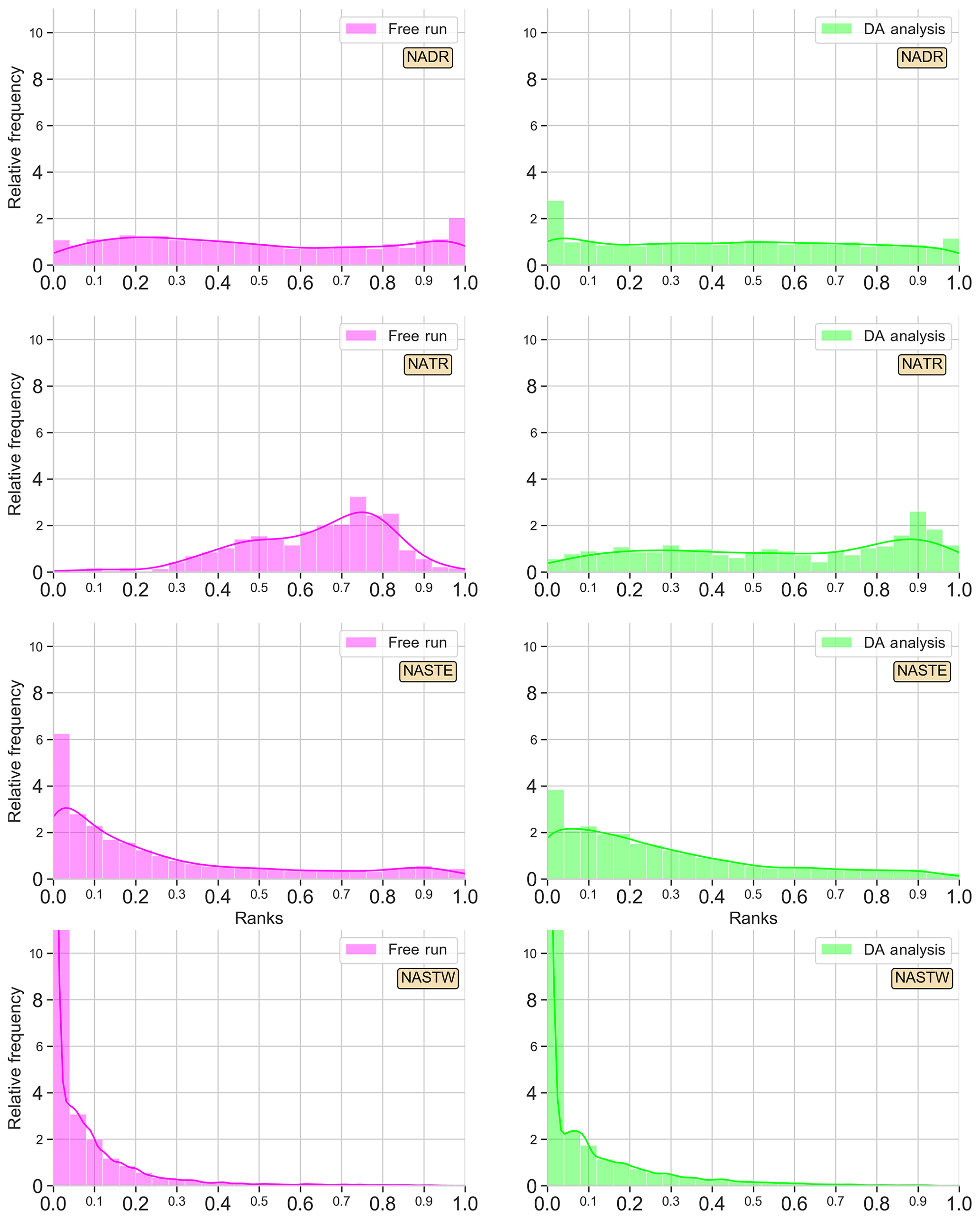
Figure 3 Surface Chl a rank histograms of the 24-member free-run experiment (magenta; left panels) and the 24-member analysis ensemble assimilation experiment (light green: right panels) in comparison with SeaWiFS data for 15 May 2005. A 30 % SeaWiFS observation error is taken into account. Longhurst provinces NADR, NATR, NASTE, and NASTW are represented.

Histograms are good indicators of how the assimilation of surface Chl a affects the probability distribution of the ensemble. The histogram for province NADR (Fig. 3 first row), which corresponds to a major part of the eastern North Atlantic temperate waters (∼40–60^∘ N, ∼10–45^∘ W), displays the good performance of the non-assimilated simulation reproducing the given observations. The histogram is flat except for a slightly tall rank “1” that indicates the highest observations are not included in the spread of the ensemble. When observations are assimilated, the distribution of ranks flattens with respect to the shape of the histogram of the non-assimilated experiment. The shape of the histogram illustrates the ensemble is now able to include the highest values of Chl a, though few ranks accumulate on the left side of the histogram.

An accumulation of ranks forms a dome in the middle of the histogram for province NATR (Fig. 3 second row), which corresponds to the southern boundary of the North Atlantic subtropical gyre (∼13–26^∘ N, ∼16–75^∘ W). The free-run surface map (see Fig. 2d–f) showed values that are too low in the northern part of the province and values that are too high in the southern part, which differ from the smooth gradient shown by the observations. When ocean color data are assimilated, the ranks' distribution becomes more homogeneous. A moderate dome of ranks on the right side of the histogram still appears, yet the envelope of the ensemble agrees well with the given observations.

The histogram of the free run shows an accumulation of ranks on the left side, i.e., too many ranks “0”, for province NASTE (Fig. 3 third row). This is the eastern branch of the subtropical gyre of the North Atlantic that goes roughly from the center of the Atlantic to the east European and African coasts (from 30 to ∼44^∘ N). The surface map (Fig. 2d–f) showed an overestimation of Chl a for most of the region, except for the oligotrophic center of the subtropical gyre where values were almost negligible. When observations are assimilated, the values of the oligotrophic area increased while values closer to the coasts tended to decrease. These corrections are also reflected into the histograms by a redistribution of the lowest ranks to the right. Nonetheless, improvements are limited, and there is an overpopulated left side of the histogram.

Lastly, the right branch of the North Atlantic subtropical gyre is included within the province NASTW (∼30–40^∘ N, ∼30–75^∘ W; Fig. 3 last row). In this area, the free-run histogram shows a strong accumulation of ranks at the left extreme; i.e, the ensemble systematically overestimates observations (positive bias). This under-dispersed shape indicates that the ensemble is unable to cover the lowest observations. In this case, the assimilation of satellite data is unable to improve the reliability of the system. Moreover, the accumulation of lower values not included within the probability distribution of the ensemble increases after assimilation.

Figure 4 Surface Chl a rank histograms of the 24-member free-run experiment (magenta; a, c, e) and the 24-member analysis ensemble assimilation experiment (light green: b, d, f) in comparison with SeaWiFS data for province NADR. Ranks are computed for 19 April, 15 May, and 5 October 2005. A 30 % SeaWiFS observation error is taken into account.

To see the time evolution of the reliability of the ensemble in the province NADR, Fig. 4 shows rank histograms computed in three different periods. A week after the initialization of the experiments, i.e., 19 April 2005, there is an accumulation of ranks on the right side of the free-run histogram (negative bias). The assimilation of satellite information redistributes ranks to the left. Yet there is still an underestimation; the probability distribution of the analysis ensemble fits better with observations, thus decreasing the bias. A month after, as we observed in Fig. 3, both the free-run and DA simulations display flat histograms indicating a good performance of the system. In particular, the system reproduces the increasing Chl a that occurs during the spring bloom period, which takes place around this date in the province (e.g., Follows and Dutkiewicz, 2001). In October, the free run tends to accumulate ranks on the right side, while an accumulation on the left side of the histogram is depicted for DA analysis. Notwithstanding, the distribution of ranks is more homogeneous after the assimilation process.

To complement reliability measurements, we present an analysis of the CRPS metrics for an in-depth evaluation of the assimilation effects. Using all daily satellite observations available during the simulation period, we calculated the Reli and Resol terms of the CRPS decomposition for provinces NADR and NASTW, two provinces with contrasting behaviors. Rank histograms (Fig. 3) showed the ensemble is consistent with observations in NADR, while it underestimates them in NASTW. Similarly, the reliability term of the CRPS metric (Fig. 5a) shows the improvements (closer to zero) made by the assimilation process on province NADR, in which the prior probability distribution was already coherent with observations. This pattern, however, reverses around August when the integration of data deteriorates the metric. This situation lasts until mid-December, when reliability for both simulations begins to coincide until the end of the experiment. By contrast, the reliability of the free-run simulation is generally closer to zero for province NASTW during the whole experiment.

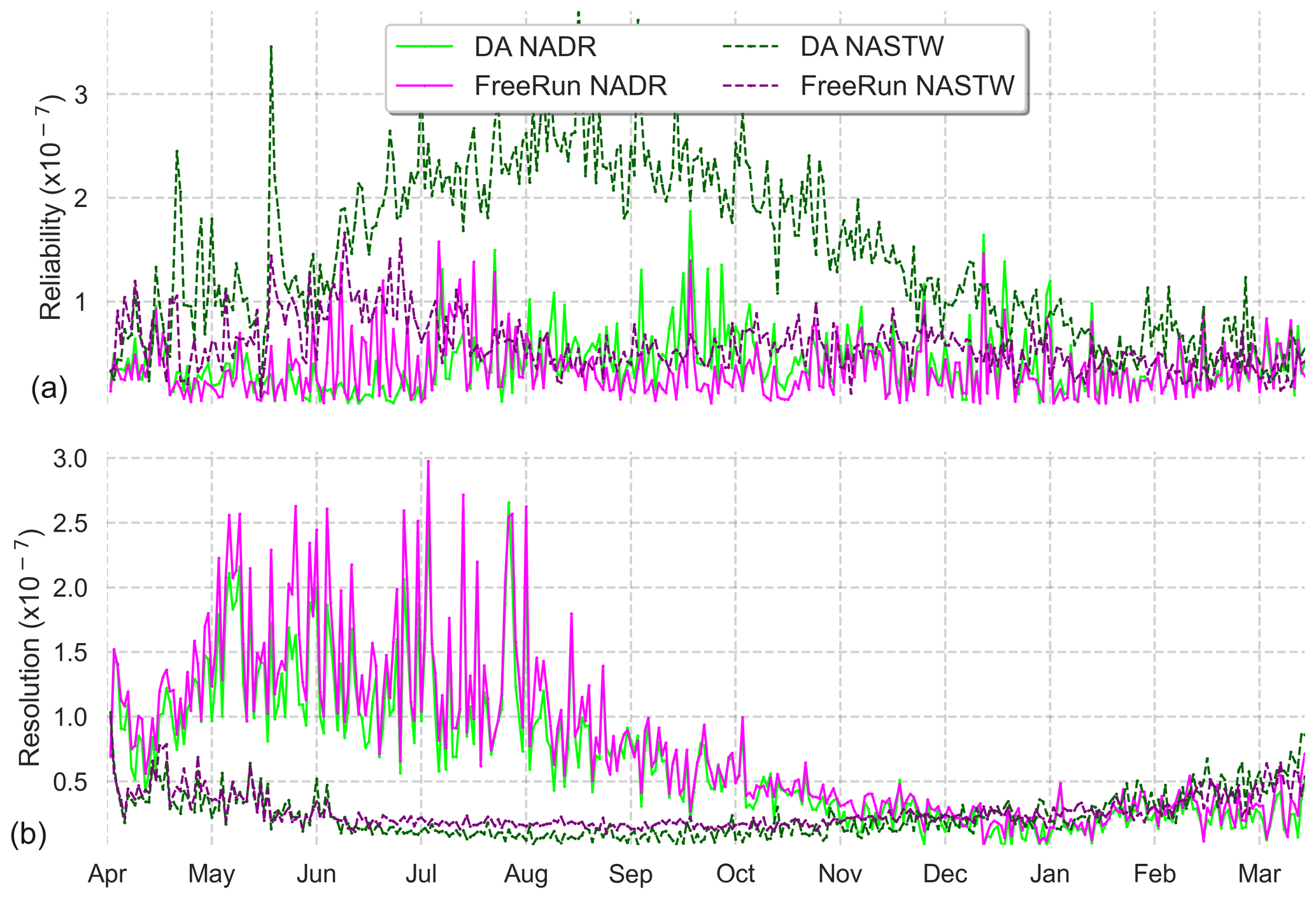
Figure 5 Time series (6 April 2005 to 5 April 2006) of reliability (a) and resolution (b) computed from CRPS decomposition for the 24-member free run (in magenta) and the 24-member forecast ensemble assimilation (in light green) experiments. Longhurst provinces NADR and NASTW are represented.

Time series of the resolution part of CRPS (Fig. 5b) show the metric is close to zero for both systems, indicating a good global performance. As expected after precedent metric diagnostics, the analysis update generally improves the resolution for province NADR. A marked seasonality is observed in the CRPS time series. During summer, the resolution of both simulations increases until the end of the season when it returns back to lower values.

3.3 Assessment of the multivariate scheme

The multivariate scheme employed here allows corrections on surface Chl a to extend to other variables. Considering a complex model such as PISCES, these changes may provoke several variables to no longer satisfy model equations, and thus results produced by these adjustments should be assessed. Moreover, surface corrections both in the observed and non-observed quantities are projected vertically onto the water column, thus altering the vertical structure of the water column. In order to evaluate the balances between Chl a and those variables that have important relations with it, such as nutrients, monthly means of nitrate and phosphate extracted from the WOA2018 data set are compared with data depicted by our simulations. Specifically, vertical profiles of Chl a and nutrient concentrations at two points placed in regions NADR and NASTW are presented (Fig. 6).

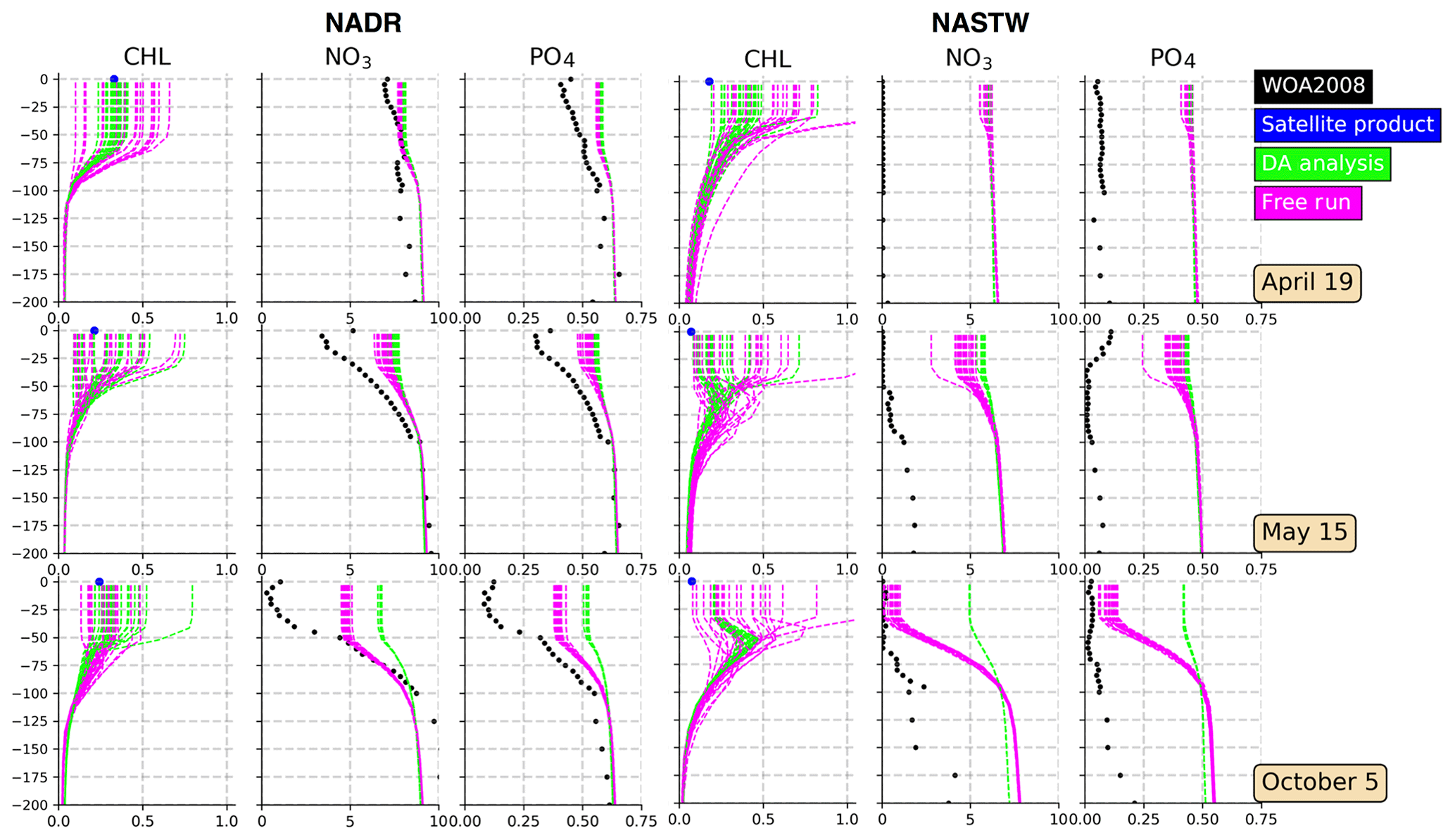
Figure 6 Vertical profiles (0–200 m) of Chl a (mg Chl m⁻³), nitrate (mmol N m⁻³), and phosphate (mmol P m⁻³) for provinces NADR (left panels; at 50^∘ N, 15^∘ W) and NASTW (right panels; at 35^∘ N, 60^∘ W) for 19 April, 15 May, and 5 October 2005. The 24-member free run (in magenta) and analysis (in green) ensembles are represented. Black dots correspond to monthly mean nitrate and phosphate concentrations extracted from the WOA2018 database. Blue dots correspond to daily mean surface Chl a obtained from the Global Ocean Satellite Observations.

Vertical profiles show that both ensembles are capable of displaying a wide range of Chl a values within the first meters of the water column. As expected, the spread of the analysis reduces, while the subsequent forecast (not shown) will restore it accordingly to match the satellite's uncertainty for the next update. The envelopes of both simulations decrease towards the bottom of the mixed layer. From there, concentrations displayed by both simulations coincide. This indicates the extent to which surface corrections are projected into the vertical. The spread of the ensemble reduces when nutrients are represented. In general, the assimilation process increases their concentrations within the mixed layer.

In the province NADR (left panels in Fig. 6), the concentrations of nutrients in the mixed-layer decrease over time. In October, mixing is close to its lowest values (Zhang et al., 2018) and so are nutrient concentrations. Inferred nutrients follow the seasonal pattern of decreasing towards October. However, their values are relatively high in comparison with climatological data. The assimilation process tends to further increase nutrient availability within the mixed layer while being capable of correctly simulating surface Chl a.

The water column is poor in nutrients in the province NASTW (right panels in Fig. 6). However, both simulations show their concentrations to be up to 7 times higher than WOA data. Weaknesses in the physical model to appropriately represent the mixed-layer dynamics in the region impair the representation of biogeochemistry as shown in Ourmières et al. (2009). As observed for province NADR, nutrient concentrations decrease towards the end of the summer. The free run simulates this decrease, especially during October when concentrations are close to observations. By contrast, the analysis moves the distribution of nutrients away from climatology. Corrections made by surface information are unable here to include the given Chl a observations. Surface data are overestimated by both ensembles. The assimilation process moves the ensemble closer to observations in the first cycles of assimilation, but it strongly overestimates them in October. The free run shows too wide a spread that reproduces Chl a concentrations up to an order of magnitude higher than satellite data.

3.4 Impact on the subtropical region

Figures presented in precedent sections indicate an erratic behavior of the system representing the transition zone between the oligotrophic subtropical area and temperate waters northwards. In order to illustrate the vertical distribution of biogeochemical properties before and after assimilation in this area, we consider meridional vertical sections of Chl a crossing the subtropical gyre and temperate waters at 45^∘ W with nutrient (nitrate+ammonium) isolines superimposed (Fig. 7). The same three dates used before are represented.

During April (Fig. 7a, b), high values of Chl a deepen up to ∼50 m depth in both experiments. However, the oligotrophic region reaches further north after the assimilation due to a deeper nutrient-depleted subsurface layer south of ∼30^∘ N. The deep Chl a maximum (DCM) of the subtropical region is placed below 100 m depth in both simulations in agreement with observational studies (Pérez et al., 2006). After assimilation, the DCM is disconnected from the subsurface maximum of temperate waters by the vertical slumping of nutrient isolines.

Figure 7 Meridional vertical sections (0–300 m) of Chl a (mg Chl m⁻³) at 25 to 50^∘ N, 45^∘ W for 19 April, 15 May, and 5 October 2005. The ensemble median of the free run (a, c, e) and the assimilated (DA analysis; b, d, f) simulations are represented. Nitrate+ammonium isolines (mmol N m⁻³) are included as solid gray lines.

A horizontal strong gradient of nutrient isolines is observed in the DA analysis section of May (Fig. 7d). Several patches of high Chl a values are evident south of ∼35^∘ N, from where the water column setting becomes similar to that displayed by the free-run simulation. These patches may be caused by the vertical propagation of surface corrections. By contrast, the free-run simulation shows a more logical distribution of parameters in which high Chl a waters are related to nutrient availability.

During October (Fig. 7e, f), differences after assimilation are more noticeable. In this period, the vertical distribution of nutrients has a key role in controlling phytoplankton growth in the region (e.g., Dutkiewicz et al., 2001), and concentrations of Chl a are relatively low as the nutricline is deep enough to limit production. Since the free run overestimates Chl a during this period in the region, the assimilation process reduces its concentrations. As a consequence, nutrients accumulate in the first 100 m of the water column north of ∼30^∘ N after the update and destabilize the equilibrium between the biomass of producers (which decreases) and the availability of nutrients (which increases). Since biogeochemical dynamics are highly dependent on this equilibrium, subsequent forecasts lead to a rapid increase in Chl a and to a severe overestimation over time that reduces the extension of the oligotrophic region to the north.

4 Discussion

4.1 Impact of the assimilation on the observed variable

The North Atlantic Ocean is a complex basin that includes a large number of biogeochemical regimes (see Fig. 1) that make it difficult to simulate using a holistic modeling system (DeYoung et al., 2004). By employing DA, we aim to reduce the impacts of model errors on the representation of ocean biogeochemistry by combining model information with available observations (Gregg et al., 2009; Ciavatta et al., 2011; Ford and Barciela, 2017). Accordingly, surface maps presented in Fig. 2 show that the assimilation process reduces the discrepancies between satellite observations and the non-assimilated free-run experiment over a major part of the domain. In particular, the DA simulation better represents values and geographical location of some structures and events such as the spring bloom period, the Gulf Stream, or phytoplankton fronts. By contrast, the assimilation scheme appears to be unable to deal with an unrealistic too abrupt front that separates the oligotrophic and temperate waters conditions (from about 25 to 35^∘ N).

By using rank histograms, we evaluate the capability of the assimilated and the free-run ensembles to agree with observations on selected Longhurst provinces (see Fig. 3). Histograms illustrate that the response of the system to the assimilation of satellite data depends upon the reliability of the prior ensemble. The assimilation process improves the statistical consistency of the system where the free-run probability distribution is homogeneous, as in the province NADR. The DA process also enhances reliability in those regions where the shape of the free-run histogram is over-dispersed, as in the province NATR. In these regions, the stochastic parameterization is enough to describe the variability of the system properly, and only a relatively small percentage of the observations lies outside of the limits of the ensemble (∼10 %). Then the assimilation process makes use of this information to increase the model skills both by reducing the dispersion and by redistributing ranks to a more homogeneous shape. The redistribution of the ensemble also increases its resolution, showing that the posterior ensemble better describes a wide variety of biogeochemical situations (see Fig. 5b).

By contrast, in regions where the prior probability distribution is strongly under-dispersed, as in the provinces NASTW and NASTE, the assimilation of satellite information is unable to raise the reliability. Since corrections are computed in the range explored by the prior ensemble, the assimilation scheme cannot correct prior distributions that exclude the full variability of the observations. In these provinces, the spread of the prior ensemble is insufficient to represent the range displayed by the observations; the ensemble consistently overestimates them during the annual cycle, and so ranks accumulate at the left extreme of the histograms (positive bias). These two provinces occupy a major part of the oligotrophic subtropical gyre of the North Atlantic where Chl a is generally low during the whole year. Since Chl a values can never become negative, the random perturbations introduced into the model formulation to create a probabilistic simulation (Garnier et al., 2016) preferentially induce an increase in Chl a concentrations.

The inability of the assimilation process to improve the skills of the simulation in these latter regions points out the necessity of appropriately defining the stochastic parameterizations of the prior PDF as a prerequisite to use DA. Particularly, uncertainties should be described accordingly with the biogeochemical characteristics of each region in order to include a major part of the observation variability.

4.2 Non-observed variables

The effects of the assimilation process to unobserved variables is a major issue in biogeochemical DA (e.g., Rousseaux and Gregg, 2012; Ciavatta et al., 2018). Several studies (e.g., Ciavatta et al., 2011) have found that the integration of surface ocean color may cause problems in the nutrient vertical distribution when a model's equation is not “plastic”, in the sense of constraining the ability of the assimilation process to correct the inferred variables. In this regard, it is important to note that our multivariate analysis scheme allows corrections of five nutrients, the Chl a content of each phytoplankton group, phytoplankton and zooplankton biomasses, and oxygen, while it only uses Chl a satellite data to constrain the ocean biogeochemistry. It is plausible that modifications on biogeochemical variables would mean that some of them would not comply with the governing model equations anymore, particularly in those regions where the model is not plastic enough to absorb modifications on the tight correlations between observed and unobserved state vectors. In some cases, these modifications may develop into simulation instabilities that can lead subsequent forecasts to deteriorate both the observed and unobserved variables (Ciavatta et al., 2011, 2018; Gregg et al., 2009). For instance, large discrepancies between observations (high concentrations of Chl a) and the model (lower concentrations) in Gregg (2008) caused their model to become unstable due to nutrient depletion. In the present case, the assimilation process has two effects on the vertical distribution of nutrients (see Figs. 6 and Fig. 7): (1) it significantly reduces the spread of the ensemble, and (2) it tends to increase their concentrations within the first ∼100 m depth.

Nutrients were not perturbed by the stochastic parameterizations (see Garnier et al., 2016), and so increases during the analysis update can only be attributed to the assimilation process. In the northern region of the North Atlantic subtropical gyre, Chl a is overestimated by the prior ensemble and so surface corrections preferentially reduce their concentrations. Since nutrients are negatively correlated with the observed variable, the corrections made by the assimilation process would increase nutrient availability. Ourmières et al. (2009) observed that the distribution of nitrate controls the biogeochemical dynamics of the subtropical region. As a consequence, the amount of nutrient available in the water column after the analysis would alter the correlations with the observed variable during the subsequent forecast in this area. If the ensemble spread were correctly established in the region, PISCES equations would be capable of absorbing these corrections. However, the ensemble has insufficient spread in the provinces NASTW and NASTE, and the increase in nutrients leads to a consistent overestimation of Chl a. By contrast, in the rest of the domain, the parameterizations of the uncertainties are consistent with observations, and the extrapolation of the assimilated information to non-observed variables works correctly. The assimilation process increases the reliability of the ensemble, and the information spreads appropriately to the rest of the variables. As a result, the subsequent daily forecast is based on an ensemble that has more appropriate spread, thus improving its general performance.

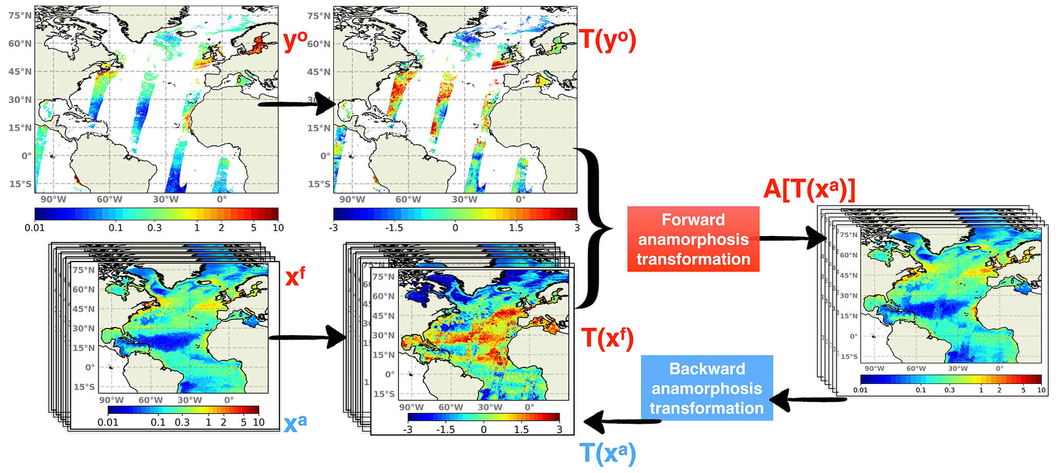
Figure 8 Schematics of the assimilation process including time-independent transformations. Both daily ensemble forecast (X^f) and daily satellite observations (y^o) are transformed by their own climatologies. Then they are projected into the anamorphic space prior to entering the analysis step. After the update, the ensemble analysis (X^a) is converted back to initialize the subsequent daily forecast.

4.3 Assimilation on fluctuations

The previous section has shown that, despite the stochastic parameterization, PISCES equations are still not plastic enough in the region north of the subtropical gyre to produce an ensemble spread that is compatible with the observations and thus to absorb the corrections made by data assimilation. A possible way to alleviate these inconsistencies without enhancing the stochastic model would be to reduce the ambition of the data assimilation system and only apply corrections to components of the observation misfit that are compatible with the ensemble spread. This approach requires a procedure to separate all model fields into two components: one component that displays uncertainties that are not correctly represented by the stochastic model, which will be kept untouched by the assimilation scheme, and another component for which the ensemble simulations can be assumed to be reliable enough to apply ensemble corrections.

In our system, in the region covered by province NASTW, the main reason for which the ensemble spread is not able to include ocean color observations is a bias in the model climatology, which is left mostly unexplained by the two sources of uncertainties that have been simulated in the stochastic model. A possible approach to reduce the ambition of data assimilation is thus to separate the model field into a climatological component and a fluctuating component and apply the assimilation process to the fluctuating component only. The main problem is then to define an operator to separate these two components.

The model climatology, on the one hand, and the observation climatology, on the other hand, can both be defined as the distribution of all values that a given variable can take over time at a given location and can be constructed by compiling all values given by the model or by the observations at that specific location. In practice, these two distributions can be described by computing a series of quantiles (for instance deciles), which can be saved as 2D or 3D fields for all model variables, on the one hand, and for all observed variables, on the other hand. The idea is then to keep the model climatology unchanged and only correct the rank of the model solution within its own climatology by assimilating the rank of the observation within the observed climatology. This means, for instance, that if an observation of Chl a falls on the first quartile of the observed climatology, then the model would be corrected to move towards the first quartile of its own climatology. In this way, the fluctuations but not the bias between the climatologies should be improved with the expected advantage of not bringing unobserved variables to unrealistic situations.

In practice, a direct solution to extract the fluctuating component is to apply the anamorphic operator transforming the climatological distribution into a normalized Gaussian distribution (with zero mean and unit variance). This can be done using the same technique used in the assimilation scheme to transform the prior ensemble into Gaussian marginal distributions. As explained in Brankart et al. (2012), the transformation operator is described by the quantiles of the probability distribution to be transformed (here the climatological distributions). Thus, as explained by the schematics in Fig. 8, observations are transformed using the quantiles of the observed climatology, and the prior ensemble is transformed using the quantiles of the model climatology. These two quantities represent the fluctuating component of the system, and the same data assimilation system (described in Sect. 2) can then be applied to this fluctuating component instead of the full field.

A 1-month assimilation experiment (TrDA) using this methodology is performed. In order to illustrate the effect of transformations on the ensemble simulation, vertical profiles of Chl a, nitrate, and phosphate are presented for 5 May 2005 (Fig. 9), the last day of the experiment. Profiles are placed in the province NASTW since the methodology aims to reduce the inconsistencies between observed and non-observed variables found in this region. Profiles illustrate that the transformed ensemble keeps the Chl a values displayed by the non-transformed simulation, while it increases the envelope of the ensemble by reproducing lower values. On the other hand, when climatologies are taken into account, the increase in the concentrations of both nitrate and phosphate after corrections is reduced. However, despite these improvements, we see that, even with the modified observational update, it is still difficult to maintain the corrections of the nutrients within reasonable bounds. Climatological variations can indeed be too wide to avoid unrealistic values occurring at a given time. Looking for a reliable synoptic ensemble with a sufficient dynamical spread to explain the full misfit to the observations of the day should thus certainly remain an important step to improve the assimilation system.

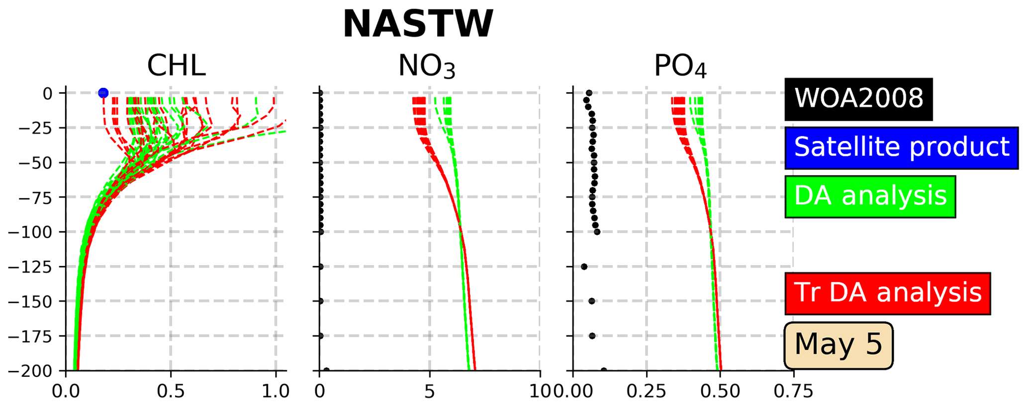
Figure 9 Vertical profiles (0–200 m) of Chl a (mg Chl m⁻³), nitrate (mmol N m⁻³) and phosphate (mmol P m⁻³) in the province NASTW (35^∘ N, 60^∘ W) for 5 May 2005. The 24-member analysis (in green) and the 24-member transformed analysis (in red) ensembles are represented. Black dots correspond to monthly mean nitrate and phosphate concentrations extracted from WOA2018 database. The blue dot corresponds to daily mean surface Chl a obtained from the Global Ocean Satellite Observations.

5 Summary and conclusions

Satellite-derived surface Chl a data are assimilated daily into a three-dimensional 24-member ensemble configuration of a coupled NEMO-PISCES model for the North Atlantic. As shown, the assimilated system has provided promising results. A regional diagnosis of a 1-year assimilation experiment has revealed that the integration of surface information increases the skills of the ensemble system in a major part of the model grid when compared to an analogous non-assimilated free-run simulation. Particularly, the assimilation of satellite data improves the representation of the surface Chl a variability both in location (upwelling areas, subtropical gyre, Gulf Stream, etc.) and seasonality (spring bloom, winter mixing, etc.). Therefore, the stochastic parameterizations introduced into the system by Garnier et al. (2016) have been shown to be adequate for undertaking DA in most of the considered domain. Where the prior ensemble includes the variability shown by the observations and their uncertainties, the assimilation process improves its probability distribution, increasing the agreement with observations (reliability) and its capability to display different community behaviors (resolution). Moreover, corrections are appropriately transferred to unobserved state vectors by the multivariate scheme.

In the northern region of the North Atlantic subtropical gyre, however, the multivariate corrections produce values that are often inconsistent with model dynamics, which can affect the correlations between the biogeochemical variables. In this region, the simulation cannot adequately absorb the corrections brought by the observations; i.e., the simulation is not plastic, and the system's performance deteriorates after the assimilation process. In particular, the analysis update increases the concentrations of nutrients, producing instabilities that lead the subsequent forecast to degrade biogeochemical fields. These results suggest that the description of uncertainties needs to be refined according to the biogeochemical characteristics of each Longhurst province.

One possible approach to reduce these instabilities would be to relax the assimilation effects on those areas. Therefore, we carried out an experiment in which corrections are only applied to the fluctuation part of the model. For that end, we apply transformations both to observations and the forecast ensemble before entering the analysis update using their climatologies. Results from a 1-month experiment show that these transformations reduce the strong effects of the assimilation, increasing nutrient concentrations in the region that lead to inconsistencies.

In addition, an improved simulation of the dynamics is needed. Ourmières et al. (2009) carried out a detailed analysis of the mixed-layer dynamics at midlatitudes. They observed that the distribution of nitrate controls the biogeochemical dynamics of the subtropical region by employing physical-only , biogeochemical-only (nitrate data), and physical–biogeochemical assimilation techniques over a coupled system. Their results showed too deep a mixed layer during March, which extended over an abnormally large area in the Gulf Stream region and its northeastern extension, and an overestimation of the stratification in the northeast Atlantic. This biased representation of the dynamics has a significant impact on the present model and should be addressed in future realizations.

Including information on biogeochemical fields in the water column in the assimilation scheme would also improve the representation of the biogeochemical state of the ocean. In situ information would be thus explicitly included by the system at depth. Nowadays, the only sources of such measurements are limited to the prospects of BGC-Argo floats (Claustre, 2009; Xing et al., 2012). Terzić et al. (2019) assimilated BGC-Argo information into a one-dimensional model and improved the DCM spatial and seasonal representation. Cossarini et al. (2019) succeed in improving the Chl a depiction over the Mediterranean Sea by assimilating vertical Chl a information supplied by BGC-Argo floats. These recent works open a horizon to constrain biogeochemical model simulations from vertical information. However, at basin scales, the current state of the network allows it to be used for validation purposes, but its limited spatial coverage makes it insufficient for assimilation procedures. In the other hand, a possibility to include nutrient information is to introduce synthetic information (e.g., Xiao and Friedrichs, 2014; Yu et al., 2018) from a non-perturbed analogue simulation. To this end, synthetic observations would be important in future efforts heading the improvement of biogeochemical data assimilation systems.