the Creative Commons Attribution 4.0 License.
the Creative Commons Attribution 4.0 License.
 | 29 Oct 2020
Seasonal and interannual variabilities of the barrier layer thickness in the tropical Indian Ocean
Xu Yuan
Xiaolong Yu
Zhongbo Su
The seasonal and interannual variations of the barrier layer thickness (BLT) in the tropical Indian Ocean (TIO) is investigated in this study using the Simple Ocean Data Assimilation version 3 (SODA v3) ocean reanalysis dataset. Analysis of this study suggests energetic but divergent seasonal variabilities of BLT in the western TIO (5∘ N–12∘ S, 55–75∘ E) and the eastern TIO (5∘ N–12∘ S, 85–100∘ E). For instance, the thicker barrier layer (BL) is observed in the western TIO during boreal winter as a result of decreasing sea surface salinity (SSS) and deeper thermocline, which are associated with the intrusion of freshwater flux and the weakened upwelling, respectively. On the contrary, the variation of BLT in the eastern TIO mainly corresponds to the variation in thermocline depth in all seasons. The interannual variability of BLT with the Indian Ocean Dipole (IOD) and El Niño–Southern Oscillation (ENSO) is explored. During the mature phase of positive IOD events, a thinner BL in the eastern TIO is attributed to the shallower thermocline, while a thicker BL appears in the western TIO due to deeper thermocline and fresher surface water. During negative IOD events, the thicker BL only occurs in the eastern TIO, corresponding to the deeper thermocline. During ENSO events, prominent BLT patterns are observed in the western TIO corresponding to two different physical processes during the developing and decaying phase of El Niño events. During the developing phase of El Niño events, the thicker BL in the western TIO is associated with deepening thermocline induced by the westward Rossby wave. During the decaying phase of El Niño events, the thermocline is weakly deepening, while the BLT reaches its maxima induced by the decreasing SSS.
- Article
(2016 KB) - Full-text XML
- BibTeX
- EndNote


The upper ocean traditionally included only the mixed layer and the thermocline. The terminology “barrier layer” (BL) was recently introduced as the mixed layer depth (MLD) was redefined from using the temperature (de Boyer Montégut et al., 2004) to using the oceanic density (Kara et al., 2000; Mignot et al., 2007). The barrier layer thickness (BLT) is simply the depth between the bottom of the mixed layer defined by density and the top of the thermocline (Lukas and Lindstrom, 1991; Masson et al., 2002; Sprintall and Tomczak, 1992). Although the BL is much thinner than the other two layers, it plays a key role in oceanic dynamics and air–sea interaction. For example, the BL helps to sustain the heat in the mixed layer by isolating the temperature in the upper ocean from the cooling entrainment. Accordingly, BL is crucial in the formation of the El Niño–Southern Oscillation (ENSO) and contributes to the formation of the different ENSO types (conventional ENSO and ENSO Modoki) (Singh et al., 2011; Maes, 2002; Maes et al., 2005, 2006). Also, the spatial structure of BLT driven by special variation in Ekman drift is crucial for the formation of monsoon cyclones in the pre-monsoon season (Thadathil et al., 2007; Vinayachandran et al., 2002; Masson et al., 2005; Neetu et al., 2012).
The variability of BLT is mainly affected by the change of MLD and thermocline due to various mechanisms, such as heavy precipitation, oceanic currents, wind stress, and oceanic waves (Bosc et al., 2009; Mignot et al., 2007; Masson et al., 2002; Qu and Meyers, 2005). For instance, a thicker BL mainly presents in the areas beneath the Intertropical Convergence Zone (ITCZ) with decreasing sea surface salinity (SSS) due to abundant rainfall (Vialard and Delecluse, 1998) or large river discharge (Pailler et al., 1999). The strong wind stress anomalies could also contribute to thickening the BL via deepening the thermocline (Seo et al., 2009).
Compared to the tropical Pacific and the Atlantic Ocean, the tropical Indian Ocean (TIO) is characterized by a shallower thermocline in the west (Yokoi et al., 2012, 2008; Yu et al., 2005) and stronger interannual variation of upper-ocean temperature in the east (Li et al., 2003; Saji et al., 1999), which provides a unique region to evaluate the seasonal and interannual variabilities of BLT.
The strong seasonality of BLT has been observed in some subregions of the TIO, such as the southeastern Arabian Sea, the Bay of Bengal, and the southeastern TIO (Schott et al., 2009). These regions are also characterized by the strong seasonality of SSS due to different hydrological processes (Rao, 2003; Subrahmanyam et al., 2011; Zhang et al., 2016; Zhang and Du, 2012). Overall, the seasonality of BLT in the TIO is partly consistent with the change of SSS due to the impact of freshwater (Masson et al., 2002; Qu and Meyers, 2005).
The interannual variability of BLT in the southeastern TIO can be partly explained by Indian Ocean Dipole (IOD) events (Qiu et al., 2012). During positive IOD year (e.g., 2006), thinner BL in the southeastern TIO is mainly led by the shallower thermocline induced by the upwelling Kelvin wave in the presence of weakly shoaling MLD. In negative IOD year (e.g., 2010), a thicker BL is expected due to the extending of the thermocline. Furthermore, at the subseasonal scale, the zonal SSS gradient driven by the freshwater advection results in a thicker BL to sustain a fresh and stable MLD (Drushka et al., 2014).
Existing studies on the interannual variability of BLT were mainly focused on specific years and lacked long-term evaluation. More importantly, the interannual variability of both thermocline and SSS are supposed to be associated with ENSO events (Grunseich et al., 2011; Rao and Sivakumar, 2003; Subrahmanyam et al., 2011; Zhang et al., 2013), but relationships between BLT and ENSO are scarcely reported in the TIO. Also, the relative impact of SSS and thermocline depth on the variability of BLT is still unclear and is not systematically investigated in the TIO. Thus, the evolution of the seasonal and interannual variabilities of BLT and its relationship with SSS and thermocline anomalies are still highly desired. The Simple Ocean Data Assimilation (SODA) version 3 ocean reanalysis dataset covers time series data from 1980 to 2015, which may be adequate for such purpose.
The remainder of this paper is arranged as follows. In Sect. 2, we briefly describe the datasets and methods. Comparisons of the BLT variability interpreted from both observed and reanalysis datasets in the TIO are presented in Sect. 3. Section 4 presents the seasonal variability of the BLT in the TIO, while its interannual variability is shown in Sect. 5. Finally, a summary and discussions are given in Sect. 6.
Two datasets are used in this study to investigate the variability of BLT in the TIO. The first one is the monthly global gridded observation and reanalysis products with 1∘ horizontal resolution from 2005 to 2015, which is compiled from Argo profiles products provided by the French Research Institute for Exploration of the Sea (Ifremer: http://www.ifremer.fr/cerweb/deboyer/mld/Subsurface_Barrier_Layer_Thickness.php, last access: June 2020). BLT is calculated as the difference between TTDDTm02 and MLD:
where TTDDTm02 is the depth of the top of thermocline, which is defined as the depth at which the surface temperature is 0.2∘ cooler than the sea surface temperature and is hereafter referred to as the isothermal layer depth (ILD). MLD is the mixed layer depth defined by oceanic density at which depth the density is 0.03 kg m−3 larger than that of the surface (de Boyer Montégut et al., 2007; Mignot et al., 2007).
Another dataset is the latest released SODA version 3 reanalysis data (1980–2015) with a horizontal resolution of 0.5∘ which is hereafter denoted as SODA v3 data and can be accessed from the Asia-Pacific Data-Research Center (APDRC: http://apdrc.soest.hawaii.edu/datadoc/soda_3.3.1.php, last access: July 2020). SODA v3 has reduced systematic errors in the upper ocean and has improved the accuracy of the poleward variability in the tropic (Carton et al., 2018). It has 26 vertical levels with a 15 m resolution near the sea surface. We adopted the same Ifremer equation to calculate SODA BLT as the difference between density and temperature-defined MLD.
Salinity and temperature in the first level (5 m) are adopted as the SODA SSS and sea surface temperature (SST), respectively. The thermocline depth is defined as the depth of the 20∘ isotherms.
Monthly SST between 1980 and 2015 on a grid of ∘ is acquired from Hadley Center Global Sea Ice and Sea Surface Temperature (HadISST: https://climatedataguide.ucar.edu/climate-data/sst-data-hadisst-v11, last access: July 2020) to calculate the Nino3.4 index. The Nino3.4 index is the average SST anomaly in the area of 5∘ N–5∘ S, 170–120∘ W. Monthly precipitation data are obtained from CMAP (Climate Prediction Center (CPC): http://apdrc.soest.hawaii.edu/las/v6/dataset?catitem=13195, last access: August 2020). Monthly zonal wind stress is obtained from SODA.
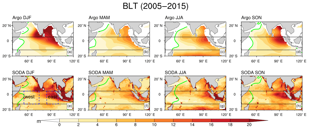
Figure 1Seasonal distributions of the BLT climatology obtained from Argo (a–d) and SODA (e–h) from 2005 to 2015 in the Indian Ocean. Units: m. The thicker green line is the zero BLT line from Argo and the dashed blue lines represent the areas of the western TIO (5∘ N–12∘ S, 55–75∘ E) and the eastern TIO (5∘ N–12∘ S, 85–100∘ E), respectively. The two thin black lines represent the latitudes of 12∘ S and 5∘ N, respectively.
The significance of simultaneous and lead–lag correlations is evaluated in this study with a Student's t test. In all the datasets, we removed the annual cycle of each parameter before the interannual correlation analysis. Composite analysis is also employed to evaluate the interannual variability of BLT using a Monte Carlo significance test. The Monte Carlo process is that the IOD/El Niño/La Niña years are randomly shuffled (10 000 times) for each month, and a mean Student's t test is used to calculate the t statistic for the selected areas. The mean of the t statistic generated by the random simulations exceeding that of the actual t value is determined and assessed at the 5 % significance level. The positive and negative IOD years are provided by the Bureau of Meteorology (http://www.bom.gov.au/climate/iod/, last access: July 2020), and the El Niño and La Niña years are obtained from the Golden Gate Weather Services (https://ggweather.com/enso/oni.htm, last access: August 2020). Monthly mean values are averaged over 3 sequential months for different seasons, e.g., December–January–February (DJF) for boreal winter, March–April–May (MAM) for boreal spring, June–July–August (JJA) for boreal summer, and September–October–November (SON) for boreal autumn. All the area-averaged parameters shown in this study are weighted by the cosine of the latitude.
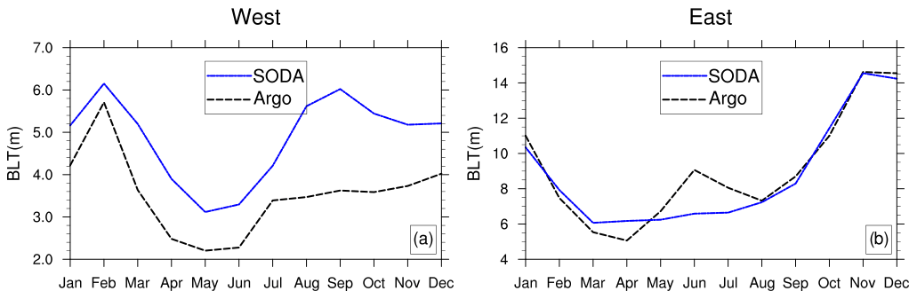
Figure 2Seasonal cycle of the region-averaged BLT for SODA and Argo: (a) the western TIO (12∘ S–5∘ N, 55–75∘ E) and (b) the eastern TIO (12∘ S–5∘ N, 85–100∘ E).
BLT in the TIO calculated from SODA v3 is first validated against Argo float observations from 2005 to 2015. As shown in Fig. 1, the seasonal BLT climatology obtained from SODA v3 is biased thinner in the Bay of Bengal in all seasons compared to that derived from Argo. This thinner BL in SODA v3 is probably because it lacks the runoff data from the Bay of Bengal as input in its reanalysis (Carton et al., 2018; Carton and Giese, 2008). Additionally, SODA BLT fails to capture the BLT feature on the west coast of Africa and the northwestern Arabian Sea (see the white areas right of the green line), where no BLT is expected due to the salinity inversion. However, for the area of interest in the TIO (5∘ N–12∘ S, 55–100∘ E), the BLT in SODA v3 shows a coherent spatial pattern with the Argo BLT, where BL is, in general, thicker in the east and thinner in the west. The seasonal evolution of BLT in the east obtained from SODA is consistent with that from Argo, shown as a decreasing trend from boreal winter to spring and an increasing trend from boreal summer to autumn.
Two subregions are highlighted to evaluate the seasonal and interannual variabilities of SODA BLT, namely western TIO (5∘ N–12∘ S, 55–75∘ E) and eastern TIO (5∘ N–12∘ S, 85–100∘ E). Since these two subregions not only represent the zonal difference of the BLT in the TIO but also include the well-known areas of the Seychelles–Chagos Thermocline Ridge (SCTR; 60–75∘ E, 12–5∘ S) and the eastern IOD area (IODE; 10∘ S–Equator, 90–100∘ E) (Manola et al., 2015; Yokoi et al., 2012, 2008). As shown in Fig. 2, region-averaged BLT obtained from SODA v3 in the western TIO is greater than that of Argo, especially during boreal summer and autumn. In the eastern TIO, SODA v3 BLT is quite comparable with that of Argo, except for slight discrepancies in June and July. The trend of BLT seasonality obtained from SODA v3 and Argo is, however, overall consistent, suggesting the robustness of using SODA v3 data in interpreting the BLT variabilities in the TIO.
Due to the insufficient temperature–salinity observations, we only compare the interannual variability of the SODA v3 BLT with Argo between 2005 and 2015. As shown in Fig. 3, the interannual variability of BLT from SODA v3 and Argo is very consistent in both the western and eastern TIO. The correlation coefficients between SODA v3 and Argo for the western and eastern TIO are 0.75 and 0.90, respectively. Results in Fig. 3 confirm that SODA v3 is adequate to evaluate the long-term seasonal and interannual variabilities of the BLT in the TIO.

Figure 3Interannual time series of the region-averaged BLT for SODA and Argo: (a) the western TIO (12∘ S–5∘ N, 55–75∘ E) and (b) the eastern TIO (12∘ S–5∘ N, 85–100∘ E).
The seasonal and interannual variations of MLD and ILD averaged over the western and eastern TIO are also presented in Fig. 4 to investigate the dominant drivers for the BLT variability. Overall, the seasonal variabilities of MLD and ILD present a consistent annual cycle in both subregions. The seasonality of BLT, however, exerts discrepancies between these two regions (Fig. 4a and b). Specifically, a semi-annual cycle of BLT is observed in the western TIO, compared to an annual cycle of BLT observed in the eastern TIO. The interannual variabilities of BLT are also different in the western and eastern TIO (Fig. 4c and d). In the western TIO, the interannual variability of BLT is more related to the ILD variation. For example, the years with thicker BL in the western TIO are associated with deeper ILD, such as 1982, 1983, 1991, and 1996. On the contrary, in the eastern TIO, the relative impact of MLD and ILD on the interannual variability of BLT cannot be discriminated. For instance, deeper BLT occurs in 1981, 1985, and 1996, corresponding to relatively shallower MLD, while the other years of deeper BLT, such as 1994, 1999, and 2001, are associated with deeper ILD. Additionally, the interannual correlation coefficients between BLT and MLD are −0.07 and −0.25 for the western and eastern TIO, respectively, and the correlations coefficients between BLT and ILD are 0.47 and 0.38 in those two subregions. The low correlation coefficients suggest that neither MLD nor ILD can fully explain the BLT variabilities in the TIO. Therefore, the difference of BLT variabilities in the western and eastern TIO needs to be further explained. In the subsequent analysis, the mixed layer variables, including SST and SSS, and thermocline depth are selected to explain the BLT variabilities in the TIO.
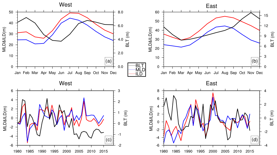
Figure 4The seasonal and interannual variations of BLT, MLD, and ILD: (a, c) the western TIO (12∘ S–5∘ N, 55–75∘ E) and (b, d) the eastern TIO (12∘ S–5∘ N, 85–100∘ E).
It is well known that the area with the thickest BL in the TIO corresponds to the freshest surface water, while the areas of the thinnest BL corresponds to the saltiest surface water (Agarwal et al., 2012; Felton et al., 2014; Han and McCreary, 2001; Vinayachandran and Nanjundiah, 2009). The spatial features of BLT and SSS in different seasons are presented in Fig. 5, where the seasonality of SSS and BLT does not co-vary, especially near the Equator. For example, surface saltier water in the western TIO elongates eastward during boreal winter and spring and retreats during boreal summer and autumn, while BLT does not vary accordingly. In the eastern TIO, BLT presents a more prominent seasonality than that of SSS, with a maximum in boreal autumn.
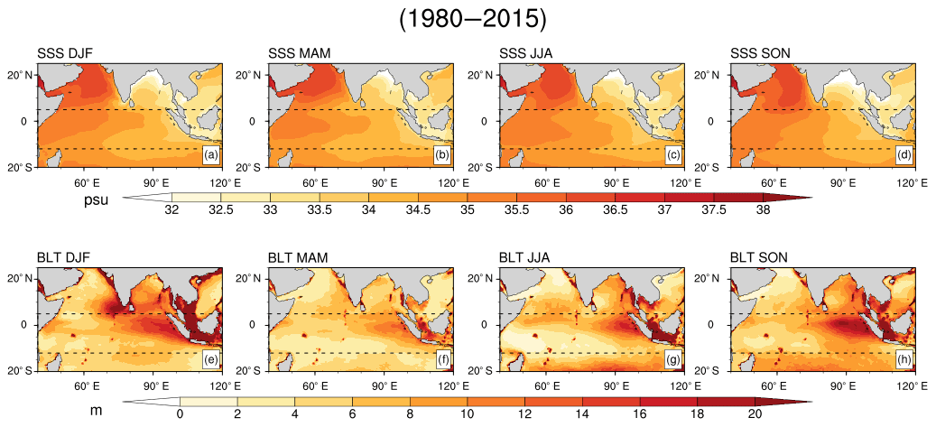
Figure 5The seasonal distributions of SSS (unit: psu; a–d) and BLT (unit: m; e–h) in the Indian Ocean from 1980 to 2015. The two dashed black lines represent the latitudes of 12∘ S and 5∘ N, respectively.
Figure 6 shows the in-phase correlations of SST and SSS anomalies with BLT anomalies. Here, the SSS, SST, and BLT anomalies have been averaged as functions of longitude vs. time in the western and eastern TIO, respectively. The seasonal BLT–SST relationship in the western TIO is not robust as only a few areas exceed the 95 % significance level (see Fig. 6a). A short-term (less than 2 months) negative correlation between BLT and SST anomalies can be observed in the eastern TIO during boreal winter. This negative BLT–SST correlation also exists when the HadISST data are employed (figure not shown). Compared with the seasonal BLT–SST relationship, the seasonal BLT–SSS relationship is more prominent in the TIO, especially in the western TIO (Fig. 6b). This negative correlation between BLT and SSS starts from January and extends to June.
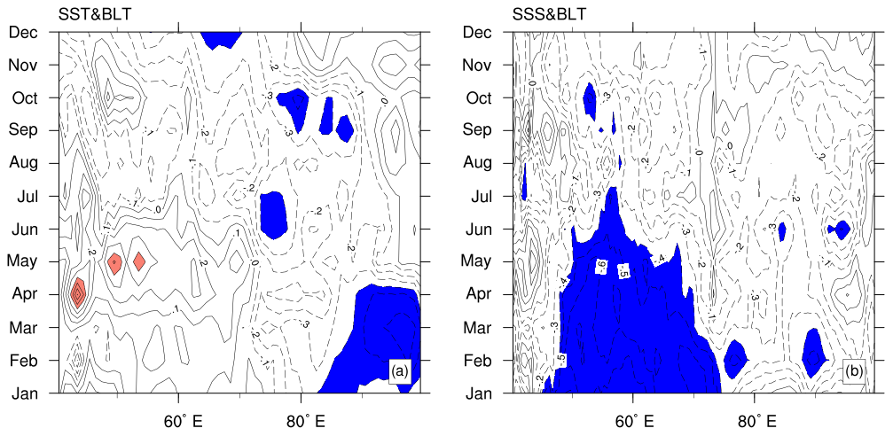
Figure 6Simultaneous correlations along the area of 12∘ S–5∘ N for (a) SST and (b) SSS anomalies with respect to BLT anomalies. Shaded areas exceed the 95 % significance level, while the shaded red and blue areas represent the areas with the positive and negative correlation coefficients, respectively.

Figure 7Lead–lag crossing correlations of BLT with SSS (a–d) and thermocline (e–h) anomalies for January (JAN), April (APR), July (JUL), and October (OCT) along the area of 12∘ S–5∘ N from 1980 to 2015. Shaded areas exceed the 95 % significance level. Positive lag means SSS (thermocline) leads BLT, and vice versa. Blue (red) shaded areas represent the negative (positive) correlation. The thick dashed black line represents the in-phase correlation.
To further understand the seasonal relationship of BLT with SSS and thermocline, we adopt the lead–lag crossing correlation analysis for BLT anomalies with respect to SSS and thermocline depth anomalies in January (JAN), April (APR), July (JUL), and October (OCT). The significant area of the lead–lag negative correlation between SSS and BLT is mainly located in the western TIO (Fig. 7a–d), which is consistent with that of their in-phase correlation (Fig. 6b). During boreal winter, spring, and autumn, the variation of SSS can affect BLT variability in the next 2 months (Fig. 7a and d). For example, fresher (saltier) water in October in the western TIO can lead to thicker (thinner) BL in November and December. The positive correlation between BLT and the thermocline depth is very prominent in the western TIO, particularly in January. The variation of the thermocline in January has an impact on BLT variations up to the next 4 months (Fig. 7e). During boreal autumn, a strong BLT–thermocline correlation mainly occurs in the eastern TIO. The variation of the thermocline in October could have an impact on BLT variations in the 3 successive months (Fig. 7h).
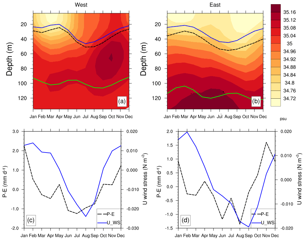
Figure 8Seasonal variation in the western TIO (12∘ S–5∘ N, 55–75∘ E) (a, c) and the eastern TIO (12∘ S–5∘ N, 85–100∘ E) (b, d). The top figures show the depth–time plots of the upper-ocean salinity (shaded), the thermocline depth (green line), isothermal layer (dashed black line), and mixed layer (blue line). The bottom figures show the freshwater flux (P−E) and zonal component of the wind stress (U_WS) anomalies in the corresponding areas.
We also examined the corresponding atmospheric forcing in the western and eastern TIO. Figure 8 shows the seasonal evolution of the upper-ocean salinity, MLD, ILD, the thermocline depth, the freshwater flux (precipitation minus evaporation, P−E), and the zonal component of the wind stress. In the western TIO, freshening of the upper-ocean water from October to April is observed due to freshwater flux, which in turn, thickens the BL, consistent with the analysis in Fig. 6b. In the meantime, a negative wind stress curl mainly dominated by the zonal wind stress leads to a weakening Ekman pumping in the western TIO. This weakened Ekman pumping inhibits the upwelling from December to April, resulting in the thicker thermocline depth (green line), which in turn, also makes the BL thicker. The driving factors of the BLT seasonality in the eastern TIO are more complex than those in the western TIO. Firstly, the seasonal evolution of SSS has a semi-annual feature, while the freshwater flux does not. This can be explained by the Indonesian Throughflow, which brings freshwater from the Pacific Ocean into the eastern TIO (Shinoda et al., 2012). Secondly, the thermocline presents the opposite seasonal cycle compared with that in the western TIO. However, the zonal wind stress displays a similar seasonal variation in both the western and eastern TIO. Last but not least, the salinity in the deeper ocean varies similarly to the thermocline depth in the eastern TIO, which is not observed in the western TIO. Thus, the freshwater flux and the wind-driven upwelling cannot fully explain the BLT seasonality in the eastern TIO. Felton et al. (2014) have suggested that the seasonal BLT variation in the eastern TIO may be related to the sea level and ILD oscillation.
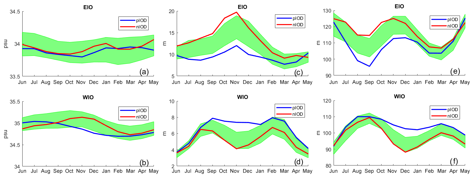
Figure 9The compositing seasonal variations of SSS (a, b; unit: psu), BLT (c, d; unit: m), and the thermocline depth (e, f; unit: m) in IOD events during the period of 1980–2015 averaged by the areas of the eastern TIO (EIO; 12∘ S–5∘ N, 85–100∘ E) and the western TIO (WIO; 12∘ S–5∘ N, 55–75∘ E), separately. The blue line represents the composite in positive IOD events and the red one represents that in negative IOD events; the green shaded area represents the 95 % Monte Carlo significance level.

The IOD, as it modifies the zonal SST gradients along the equatorial TIO, is a crucial climate mode on the interannual scale (Schott et al., 2009). IOD events mostly develop and mature within boreal autumn and decay in boreal winter (Saji et al., 1999). The IOD corresponds well with local precipitation and wind change and has an impact on the SSS (Saji and Yamagata, 2003). The intensity of IOD can be defined by the Dipole Mode Index (DMI), which is the difference between SST anomalies in the region of 10∘ S–10∘ N, 50–70∘ E, and 10∘ S–Equator, 90–110∘ E (Saji et al., 1999). Based on the DMI, we composited the monthly SSS, BLT, and the thermocline depth anomalies for positive IOD (pIOD) and negative IOD (nIOD) events, respectively. The corresponding years are listed in Table 1. Figure 9 presents the composited seasonal variations for our current dataset during the period of 1980–2015. The Monte Carlo procedure has been used to evaluate the significance of the composite variations (green shaded areas). If the value of the variables exceeds the green shaded areas, it is assessed to be significant at the 95 % significance level. In the eastern TIO (Fig. 9a, c, and e), there are no prominent patterns of SSS during negative (positive) IOD events. This is because the eastward (westward) saltier (fresher) water advection can compensate for the reduced (increased) precipitation due to the presence of the strong Wyrtki jet (Thompson et al., 2006). In contrast, the thermocline and BLT display a prominent seasonal phase-locking feature in the eastern TIO. Specifically, during the mature and decaying phases of the positive IOD events, shallower thermocline depth due to strong upwelling leads to thinner BL. This thinner BL provides favorable circumstances for the cold water intrusion into the ocean surface, which contributes to the intensification of positive IOD events (Deshpande et al., 2014). During the mature phase of negative IOD events, a deeper thermocline along with a thicker BL could be observed in the eastern TIO due to the strong downwelling. In the western TIO (Fig. 9b, d, and f), the thicker BL prominently occurs only during the mature phase of positive IOD events that are associated with deeper thermocline and fresher surface water. The deeper thermocline is due to wind-induced downwelling and the fresher surface water is attributed to the westward freshwater advection and more precipitation induced by positive IOD events in the western TIO.
Table 1List of positive IOD events and negative IOD events in our study period.
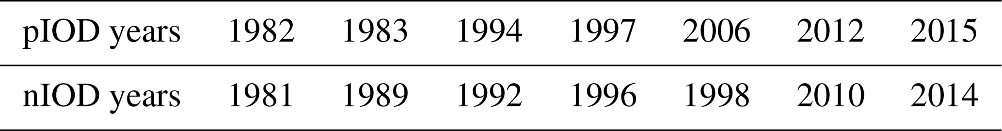
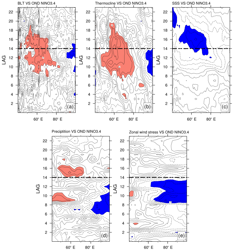
Figure 11Lagged correlations of (a) BLT, (b) the thermocline depth, (c) SSS, (d) precipitation, and (e) the zonal wind stress anomalies averaged in 12∘ S–5∘ N, with the Nino3.4 index as a function of longitude and calendar month (shaded areas exceed the 95 % significance level; positive lagging correlations are shaded in red and negative ones are in blue; the thick dashed black line represents the start of the decaying phase of El Niño).
In previous studies, a significant seasonal phase-locking impact of ENSO on the TIO has been addressed (Schott et al., 2009; Zhang and Yang, 2007). This seasonal phase-locking impact mainly exists during the developing phase of ENSO (boreal autumn), the mature phase of ENSO (boreal winter), and the decaying phase of ENSO (boreal spring) in different areas of the TIO. We composited our variables based on ENSO events from Table 2. Figure 10 presents the composited results of the seasonal variation of BLT, SSS, and thermocline. The thinner BL is mainly associated with shallower thermocline during the developing and mature phases of El Niño (Fig. 10c and e), which can be explained by the anomalous easterlies along the Equator invoked by the adjusted Walker circulation (Alexander et al., 2002; Kug and Kang, 2006). In the western TIO, thicker BL presents two peaks during the developing and decaying phase of El Niño events (Fig. 10d). The first peak of thicker BLT corresponds to a peak of deepening thermocline depth due to the westward downwelling Rossby wave and the anomalous wind stress induced by El Niño (Kug and Kang, 2006; Xie et al., 2002). The second peak of thicker BL is more significant, which connects to the peak of the deepening thermocline and decreasing SSS (Fig. 10b and f).
Table 2List of El Niño events and La Niña events in our study period.
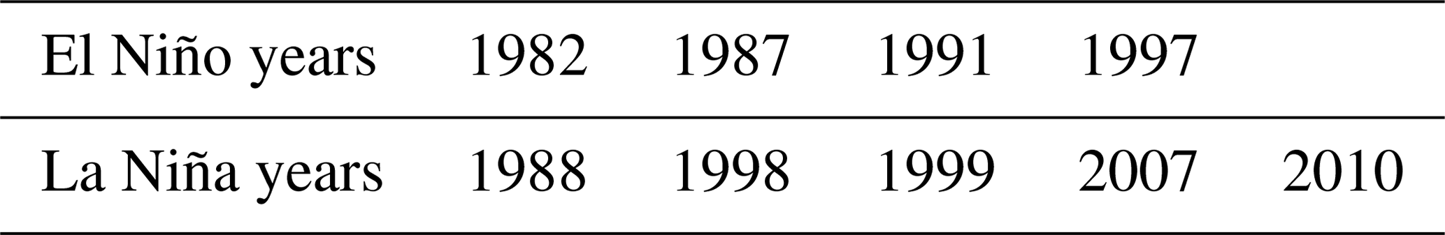
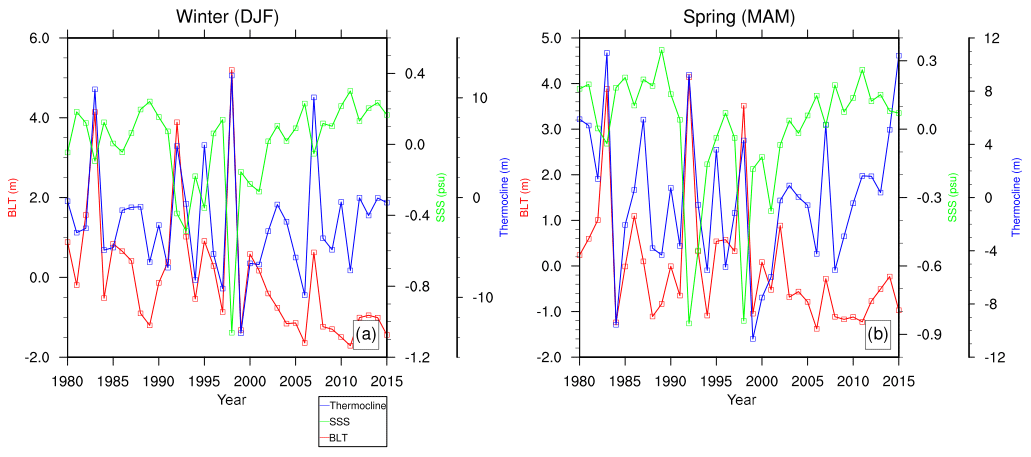
Figure 12Time series of BLT, SSS, and thermocline anomalies averaged over the western TIO (12∘ S–5∘ N, 55–75∘ E) during boreal winter (a) and spring (b) from 1980 to 2015. Red, green, and blue lines represent BLT, SSS, and the thermocline depth, respectively.
The pattern of BLT in the western TIO during El Niño events is the most prominent, and its two peaks can be explained by two physical mechanisms. Thus, we calculate the lead–lag correlations between the BLT, thermocline, and SSS anomalies and the Nino3.4 index from 1980 to 2015 to investigate the BLT–El Niño relationship. The correlation coefficients between the thermocline depth anomalies and the Nino3.4 index reach significant values during the mature period of El Niño (Fig. 11b). Also, the correlation between thermocline and Nino3.4 index shows a time delay that is longitude dependent, which is consistent with the result of Xie et al. (2002). This deeper thermocline due to the westward downwelling Rossby wave induced by El Niño affects the corresponding BL. As shown in Fig. 11a, there is a remarkably positive correlation between BLT and the Nino3.4 index 1 month apart. Then, the correlation between the thermocline depth anomalies and El Niño becomes weaker during the decaying period of El Niño (Fig. 11b). However, there is an enlarged area of correlation between BLT and ENSO. This enlarged pattern accompanies with the appearance of a negative correlation between SSS and ENSO (Fig. 11c). The negative SSS anomalies due to precipitation induced by El Niño via the adjusting Walker circulation and the westward Rossby wave in the western TIO thicken the BLT anomalies (Fig. 11d and e).
To further verify the impact of IOD and ENSO events on the interannual variation of BLT, the time series of BLT, SSS, and thermocline anomalies averaged over the western TIO during boreal winter and spring from 1980 to 2015 are shown in Fig. 12. During boreal winter (Fig. 12a), thicker BL and deeper thermocline could be found in 1983, 1992, and 1998, corresponding to the mature phase of El Niño events (Table 2). During boreal spring (Fig. 12b), thicker BL and deeper thermocline could also be observed in the decaying phase of El Niño events, accompanied with fresher surface water. On the other hand, the effect of IOD on the interannual variability of BLT could also be observed in specific years, such as 1983, 1998, and 2006 (Table 1).
The seasonal and interannual variabilities of BLT in the TIO are investigated by using the SODA v3 ocean reanalysis dataset. SODA v3 reasonably well reproduces the observed mean and variabilities of BLT in the TIO when compared to Argo.
The dominant contributors to the BLT seasonality are different in the western and eastern TIO. BLT in the eastern TIO is positively correlated with the thermocline depth during boreal autumn, winter, and spring, and the positive impact can last for the next 3–4 months. On the other hand, BLT in the western TIO is negatively correlated with SSS during boreal winter, spring, and autumn. The change of SSS can further control BLT variation in up to 2 subsequent months. Additionally, the change of BLT in the western TIO during boreal winter can also be affected by the variation of the thermocline depth. For instance, during boreal winter, fresher surface water and shallower thermocline depth result in thicker BL in the western TIO; these result from freshwater flux and strong wind convergence induced by both the winter monsoon wind and the westerlies (Yokoi et al., 2012).
The interannual variability of BLT exerts a seasonal phase-locking pattern during the IOD and ENSO years. In the eastern TIO, the thicker BL is led by the deeper thermocline due to wind-induced downwelling during the mature phase of negative IOD events. In contrast, the thinner BL is dominated by the shallower thermocline due to wind-induced upwelling during the developing and mature phases of positive IOD events. In the western TIO, the thicker BL is only observed during the mature and decaying phases of positive IOD events, along with deeper thermocline and fresher surface water.
The prominent patterns of BLT in the western TIO can only be detected during El Niño events. According to the theory of Xie et al. (2002), warmer water developing in the eastern tropical Pacific Ocean (El Niño) results in anomalous easterlies and the generation of the downwelling Rossby wave along the equatorial TIO. Thereby, the thermocline depth is deepened in the western TIO, resulting in the thicker BL. This thickening BL hampers the upwelling process and helps to sustain warmer SST. During the decaying phase of El Niño events, there is an anomalous ascending branch of the adjusted Walker circulation in the western TIO. As a result, SSS in the western TIO decreases due to abundant precipitation. Consequently, fresher surface water contributes to thickening the BL, which in turn sustains the warmer SST in the western TIO.
The code is available from the authors upon request (NCL and MATLAB).
The gridded ocean parameter datasets are available at the Asian-Pacific Data-Research Center (http://apdrc.soest.hawaii.edu/data/data.php, APDRC, 2020) and National Oceanic and Atmospheric Administration (https://www.esrl.noaa.gov/psd/data/gridded/data.noaa.oisst.v2.html, National Oceanic and Atmospheric Administration Physical Sciences Laboratory, 2020).
XuY designed the study, carried out the analysis presented, and drafted the manuscript. ZS supervised the project, providing edits to the manuscript. XiY helped to edit the manuscript.
The authors declare that they have no conflict of interest.
We thank A. J. George Nurser and one anonymous reviewer for their constructive comments to improve the manuscript. The use of the following datasets is gratefully acknowledged: the gridded ocean parameter datasets are available at the Asian-Pacific Data-Research Center (http://apdrc.soest.hawaii.edu/data/data.php, last access: August 2020) and National Oceanic and Atmospheric Administration (https://www.esrl.noaa.gov/psd/data/gridded/data.noaa.oisst.v2.html, last access: August 2020).
The article processing charges for this open-access publication were covered by WRS department in faculty of Geo-Information Science and Earth Observation (ITC) in University of Twente.
This paper was edited by A. J. George Nurser and reviewed by one anonymous referee.
Agarwal, N., Sharma, R., Parekh, A., Basu, S., Sarkar, A., and Agarwal, V. K.: Argo observations of barrier layer in the tropical Indian Ocean, Adv. Space Res., 50, 642–654, 2012.
Alexander, M. A., Bladé, I., Newman, M., Lanzante, J. R., Lau, N.-C., and Scott, J. D.: The atmospheric bridge: The influence of ENSO teleconnections on air–sea interaction over the global oceans, J. Climate, 15, 2205–2231, 2002.
APDRC – Asia-Pacific Data Research Center of the IPRC: Argo, SODA and CMAP, available at: http://apdrc.soest.hawaii.edu/data/data.php, last access: August 2020.
Bosc, C., Delcroix, T., and Maes, C.: Barrier layer variability in the western Pacific warm pool from 2000 to 2007, J. Geophys. Res.-Oceans, 114, C06023, https://doi.org/10.1029/2008JC005187, 2009.
Carton, J. A. and Giese, B. S.: A reanalysis of ocean climate using Simple Ocean Data Assimilation (SODA), Mon. Weather Rev., 136, 2999–3017, 2008.
Carton, J. A., Chepurin, G. A., and Chen, L.: SODA3: a new ocean climate reanalysis, J. Climate, 31, 6967–6983, 2018.
de Boyer Montégut, C., Madec, G., Fischer, A. S., Lazar, A., and Iudicone, D.: Mixed layer depth over the global ocean: An examination of profile data and a profile-based climatology, J. Geophys. Res.-Oceans, 109, C12003, https://doi.org/10.1029/2004JC002378, 2004.
de Boyer Montégut, C., Mignot, J., Lazar, A., and Cravatte, S.: Control of salinity on the mixed layer depth in the world ocean: 1. General description, J. Geophys. Res.-Oceans, 112, C06011, https://doi.org/10.1029/2006JC003953, 2007.
Deshpande, A., Chowdary, J., and Gnanaseelan, C.: Role of thermocline-SST coupling in the evolution of IOD events and their regional impacts, Clim. Dynam., 43, 163–174, 2014.
Drushka, K., Sprintall, J., and Gille, S. T.: Subseasonal variations in salinity and barrier-layer thickness in the eastern equatorial Indian Ocean, J. Geophys. Res.-Oceans, 119, 805–823, 2014.
Felton, C. S., Subrahmanyam, B., Murty, V., and Shriver, J. F.: Estimation of the barrier layer thickness in the Indian Ocean using Aquarius Salinity, J. Geophys. Res.-Oceans, 119, 4200–4213, 2014.
Grunseich, G., Subrahmanyam, B., Murty, V., and Giese, B. S.: Sea surface salinity variability during the Indian Ocean Dipole and ENSO events in the tropical Indian Ocean, J. Geophys. Res.-Oceans, 116, C11013, https://doi.org/10.1029/2011JC007456, 2011.
Han, W. and McCreary, J. P.: Modeling salinity distributions in the Indian Ocean, J. Geophys. Res., 106, 859–877, 2001.
Kara, A. B., Rochford, P. A., and Hurlburt, H. E.: An optimal definition for ocean mixed layer depth, J. Geophys. Res.-Oceans, 105, 16803–16821, 2000.
Kug, J.-S. and Kang, I.-S.: Interactive feedback between ENSO and the Indian Ocean, J. Climate, 19, 1784–1801, 2006.
Li, T., Wang, B., Chang, C., and Zhang, Y.: A theory for the Indian Ocean dipole–zonal mode, J. Atmos. Sci., 60, 2119–2135, 2003.
Lukas, R. and Lindstrom, E.: The mixed layer of the western equatorial Pacific Ocean, J. Geophys. Res.-Oceans, 96, 3343–3357, 1991.
Maes, C.: Salinity barrier layer and onset of El Niño in a Pacific coupled model, Geophys. Res. Lett., 29, 59-1–59-4, 2002.
Maes, C., Picaut, J., and Belamari, S.: Importance of the salinity barrier layer for the buildup of El Niño, J. Climate, 18, 104–118, 2005.
Maes, C., Ando, K., Delcroix, T., Kessler, W. S., McPhaden, M. J., and Roemmich, D.: Observed correlation of surface salinity, temperature and barrier layer at the eastern edge of the western Pacific warm pool, Geophys. Res. Lett., 33, L06601, https://doi.org/10.1029/2005GL024772, 2006.
Manola, I., Selten, F., de Ruijter, W., and Hazeleger, W.: The ocean-atmosphere response to wind-induced thermocline changes in the tropical South Western Indian Ocean, Clim. Dynam., 45, 989–1007, 2015.
Masson, S., Delecluse, P., Boulanger, J. P., and Menkes, C.: A model study of the seasonal variability and formation mechanisms of the barrier layer in the eastern equatorial Indian Ocean, J. Geophys. Res.-Oceans, 107, SRF 18-11–SRF 18-20, 2002.
Masson, S., Luo, J. J., Madec, G., Vialard, J., Durand, F., Gualdi, S., Guilyardi, E., Behera, S., Delécluse, P., and Navarra, A.: Impact of barrier layer on winter-spring variability of the southeastern Arabian Sea, Geophys. Res. Lett., 32, L07703, https://doi.org/10.1029/2004GL021980, 2005.
Mignot, J., de Boyer Montégut, C., Lazar, A., and Cravatte, S.: Control of salinity on the mixed layer depth in the world ocean: 2. Tropical areas, J. Geophys. Res.-Oceans, 112, C10010, https://doi.org/10.1029/2006JC003953, 2007.
National Oceanic and Atmospheric Administration Physical Sciences Laboratory: NOAA Optimum Interpolation (OI) Sea Surface Temperature (SST) V2, available at: https://www.esrl.noaa.gov/psd/data/gridded/data.noaa.oisst.v2.html, last access: August 2020.
Neetu, S., Lengaigne, M., Vincent, E. M., Vialard, J., Madec, G., Samson, G., Ramesh Kumar, M., and Durand, F.: Influence of upper-ocean stratification on tropical cyclone-induced surface cooling in the Bay of Bengal, J. Geophys. Res.-Oceans, 117, C12020, https://doi.org/10.1029/2012JC008433, 2012.
Pailler, K., Bourlès, B., and Gouriou, Y.: The barrier layer in the western tropical Atlantic Ocean, Geophys. Res. Lett., 26, 2069–2072, 1999.
Qiu, Y., Cai, W., Li, L., and Guo, X.: Argo profiles variability of barrier layer in the tropical Indian Ocean and its relationship with the Indian Ocean Dipole, Geophys. Res. Lett., 39, L08605, https://doi.org/10.1029/2012GL051441, 2012.
Qu, T. and Meyers, G.: Seasonal variation of barrier layer in the southeastern tropical Indian Ocean, J. Geophys. Res.-Oceans, 110, C11003, https://doi.org/10.1029/2004JC002816, 2005.
Rao, R. and Sivakumar, R.: Seasonal variability of sea surface salinity and salt budget of the mixed layer of the north Indian Ocean, J. Geophys. Res.-Oceans, 108, 9-1–9-14, 2003.
Rao, R. R. and Sivakumar, R.: Seasonal variability of sea surface salinity and salt budget of the mixed layer of the north Indian Ocean, J. Geophys. Res., 108, C13009, https://doi.org/10.1029/2001JC000907, 2003.
Saji, N., Goswami, B. N., Vinayachandran, P., and Yamagata, T.: A dipole mode in the tropical Indian Ocean, Nature, 401, 360–363, 1999.
Saji, N. H. and Yamagata, T.: Possible impacts of Indian Ocean dipole mode events on global climate, Climate Res., 25, 151–169, 2003.
Schott, F. A., Xie, S.-P., and McCreary, J. P.: Indian Ocean circulation and climate variability, Rev. Geophys., 47, RG1002, https://doi.org/10.1029/2007RG000245, 2009.
Seo, H., Xie, S.-P., Murtugudde, R., Jochum, M., and Miller, A. J.: Seasonal effects of Indian Ocean freshwater forcing in a regional coupled model, J. Climate, 22, 6577–6596, 2009.
Shinoda, T., Han, W., Metzger, E. J., and Hurlburt, H. E.: Seasonal variation of the Indonesian throughflow in Makassar Strait, J. Phys. Oceanogr., 42, 1099–1123, 2012.
Singh, A., Delcroix, T., and Cravatte, S.: Contrasting the flavors of El Niño – Southern Oscillation using sea surface salinity observations, J. Geophys. Res.-Oceans, 116, C06016, https://doi.org/10.1029/2010JC006862, 2011.
Sprintall, J. and Tomczak, M.: Evidence of the barrier layer in the surface layer of the tropics, J. Geophys. Res.-Oceans, 97, 7305–7316, 1992.
Subrahmanyam, B., Murty, V., and Heffner, D. M.: Sea surface salinity variability in the tropical Indian Ocean, Remote Sens. Environ., 115, 944–956, 2011.
Thadathil, P., Muraleedharan, P. M., Rao, R. R., Somayajulu, Y. K., Reddy, G. V., and Revichandran, C.: Observed seasonal variability of barrier layer in the Bay of Bengal, J. Geophys. Res.-Oceans, 112, C02009, https://doi.org/10.1029/2006JC003651, 2007.
Thompson, B., Gnanaseelan, C., and Salvekar, P.: Variability in the Indian Ocean circulation and salinity and its impact on SST anomalies during dipole events, J. Mar. Res., 64, 853–880, 2006.
Vialard, J. and Delecluse, P.: An OGCM study for the TOGA decade. Part II: Barrier-layer formation and variability, J. Phys. Oceanogr., 28, 1089–1106, 1998.
Vinayachandran, P., Murty, V., and Ramesh Babu, V.: Observations of barrier layer formation in the Bay of Bengal during summer monsoon, J. Geophys. Res.-Oceans, 107, SRF 19-11–SRF 19-19, 2002.
Vinayachandran, P. N. and Nanjundiah, R. S.: Indian Ocean sea surface salinity variations in a coupled model, Clim. Dynam., 33, 245–263, 2009.
Xie, S.-P., Annamalai, H., Schott, F. A., and McCreary Jr., J. P.: Structure and mechanisms of South Indian Ocean climate variability, J. Climate, 15, 864–878, 2002.
Yokoi, T., Tozuka, T., and Yamagata, T.: Seasonal variation of the Seychelles Dome, J. Climate, 21, 3740–3754, 2008.
Yokoi, T., Tozuka, T., and Yamagata, T.: Seasonal and interannual variations of the SST above the Seychelles Dome, J. Climate, 25, 800–814, 2012.
Yu, W., Xiang, B., Liu, L., and Liu, N.: Understanding the origins of interannual thermocline variations in the tropical Indian Ocean, Geophys. Res. Lett., 32, L24706, https://doi.org/10.1029/2005GL024327, 2005.
Zhang, N., Feng, M., Du, Y., Lan, J., and Wijffels, S. E.: Seasonal and interannual variations of mixed layer salinity in the southeast tropical Indian Ocean, J. Geophys. Res.-Oceans, 121, 4716–4731, 2016.
Zhang, Q. and Yang, S.: Seasonal phase-locking of peak events in the eastern Indian Ocean, Adv. Atmos. Sci., 24, 781–798, 2007.
Zhang, Y. and Du, Y.: Seasonal variability of salinity budget and water exchange in the northern Indian Ocean from HYCOM assimilation, Chin. J. Oceanol. Limn., 30, 1082–1092, 2012.
Zhang, Y., Du, Y., Zheng, S., Yang, Y., and Cheng, X.: Impact of Indian Ocean Dipole on the salinity budget in the equatorial Indian Ocean, J. Geophys. Res.-Oceans, 118, 4911–4923, 2013.