the Creative Commons Attribution 4.0 License.
the Creative Commons Attribution 4.0 License.
 | 27 Oct 2020
Sea-ice and water dynamics and moonlight impact the acoustic backscatter diurnal signal over the eastern Beaufort Sea continental slope
Igor A. Dmitrenko
Vladislav Petrusevich
Gérald Darnis
Sergei A. Kirillov
Alexander S. Komarov
Jens K. Ehn
Alexandre Forest
Louis Fortier
Søren Rysgaard
David G. Barber
A 2-year-long time series of currents and acoustic backscatter from an acoustic Doppler current profiler, moored over the eastern Beaufort Sea continental slope from October 2003 to September 2005, were used to assess the dynamics and variability of the sound-scattering layer. It has been shown that acoustic backscatter is dominated by a synchronized diel vertical migration (DVM) of zooplankton. Our results show that DVM timings (i) were synchronous with sunlight and (ii) were modified by moonlight and sea ice, which attenuates light transmission to the water column. Moreover, DVM is modified or completely disrupted during highly energetic current events. Thicker ice observed during winter–spring 2005 lowered the backscatter values but favored extending DVM toward the midnight sun. In contrast to many previous studies, DVM occurred through the intermediate water layer during the ice-free season of the midnight sun in 2004. In 2005, the midnight-sun DVM was likely impacted by a high acoustic scattering generated by suspended particles. During full moon at low cloud cover, the nighttime moonlight illuminance led to zooplankton avoidance of the subsurface layer, disrupting DVM. Moreover, DVM was disrupted by upwelling, downwelling, and eddy passing. We suggest that these deviations are consistent with DVM adjusting to avoid enhanced water dynamics. For upwelling and downwelling, zooplankton likely respond to the along-slope water dynamics dominated by surface- and depth-intensified flow, respectively. This drives zooplankton to adjust DVM by aggregating in the low or upper intermediate water layer for upwelling and downwelling, respectively. The baroclinic eddy reversed DVM below the eddy core.
- Article
(25743 KB) - Full-text XML
- BibTeX
- EndNote


The acoustic backscatter signal recorded in the ocean by acoustic Doppler current profilers (ADCPs) is mainly dominated by zooplankton. The diurnal patterns of the acoustic backscatter signal are comprised of diel vertical migration (DVM) of zooplankton, which is synchronized movement of zooplankton up and down in the water column over a daily cycle (e.g., Brierley, 2014). In terms of biomass, DVM is arguably the largest daily migration of animals on Earth (Hays, 2003) and the largest nonhuman migration (Brierley et al., 2014). DVM has been extensively explored in the Arctic using either echo sounders or zooplankton nets (e.g., Kosobokova, 1978; Fortier, et al., 2001; Blachowiak-Samolyk et al., 2006; Cottier et al., 2006; Falk-Petersen et al., 2008). The latest progress in assessing DVM in the Arctic is related to understanding DVM during the Arctic polar night (Berge et al., 2009, 2015) and the role of moonlight in modifying DVM (Last et al., 2016; Petrusevich et al., 2016). While significant progress has been achieved in understanding DVM, the sea-ice and ocean dynamic control on DVM in the Arctic environment remains poorly appreciated.
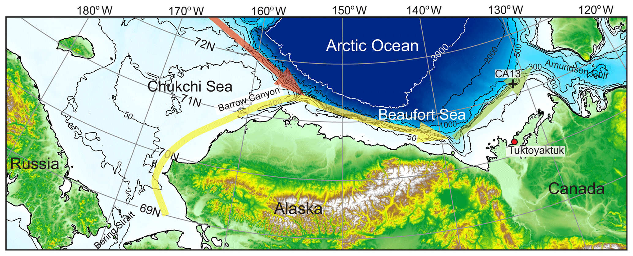
Figure 1Map of the Beaufort Sea with the location of the ArcticNet mooring CA13 (black numbered cross). Thick red, yellow, and green arrows show circulation associated with the shelf-break jet over the Chukchi Sea and western and eastern Beaufort Sea, respectively.
ADCPs moored over the entire annual cycle in the seasonally ice-covered Arctic water provide a unique temporal evolution of the DVM patterns. This seasonal perspective is essential to achieve a more complete and quantitative understanding of DVM in response to the light and sea-ice conditions (e.g., Tran et al., 2016; Hobbs et al., 2018). Here we assess the temporal evolution of DVM patterns using a 2-year-long time series of velocity and acoustic backscatter from an ADCP-equipped mooring deployed over the upper eastern Beaufort Sea continental slope from October 2003 to September 2005 (Fig. 1). The ADCP limitation, however, comes from its ability to detect only the biomass moving at a population level, i.e., comprising the migrating sound-scattering layer (Hobbs et al., 2018).
The oceanographic factors controlling DVM in the seasonally ice-covered Arctic areas, located at the inner border of the polar circle, remain poorly assessed. Here we use observations from the oceanographic mooring located at ∼71∘ N, the area where the Sun is between 0 and >6∘ below the horizon all day on the winter solstice. At this latitude no actual daylight is experienced during short winter daylight hours, with the exception of civil twilight when solar illumination is still sufficient for the human eye to distinguish terrestrial objects. This geographical position makes our DVM observational site vastly different from those at Svalbard (astronomical twilight; the Sun is between 12 and 18∘ below the horizon at ∼80∘ N; e.g., Grenvald et al., 2016; Darnis et al., 2017), Canada Basin (nautical twilight; the Sun is between 6 and 12∘ below the horizon at ∼77.5∘ N; La et al., 2018), and northeast Greenland (nautical twilight, ∼74.5∘ N; Petrusevich et al., 2016). Civil twilight is observed at the CA13 latitude from 19 November to 21 January. For the winter solstice (22 December), the civil twilight lasts for about 3 h. The polar day (or the midnight sun; the Sun is above the horizon for the entire 24 h) lasts at the CA13 latitude from 10 May to 1 August.
This study is built on results by Dmitrenko et al. (2018) on water dynamics over the eastern Beaufort Sea continental slope, taking advantage of using the ADCP-derived acoustic backscatter for temporal appreciation of DVM patterns during two consecutive annual cycles. Our particular focus is on the DVM modifications caused by wind-forced upwelling and downwelling over the Beaufort Sea continental slope and the different types of sea-ice cover. We also add more data points and further proof to research focused on the effect of moonlight on DVM (e.g., Webster et al., 2015; Last et al., 2016; Petrusevich et al., 2016).
We used data from the ArcticNet oceanographic mooring CA13 deployed over the upper Canadian Beaufort Sea continental slope at 300 m of depth from 9 October 2003 to 4 September 2005 at 71∘21.356′ N, 131∘21.824′ W (Fig. 1). The mooring description can be found in Dmitrenko et al. (2016). For this study, we used (i) velocity and acoustic backscatter intensity records from a 300 kHz upward-looking Workhorse Sentinel ADCP by Teledyne RD Instruments (RDI) at 119 m of depth and (ii) temperature records from the moored CTD (conductivity–temperature–depth) SBE-37 by Sea-Bird Electronics, Inc., at 49 and 119 m of depth. The velocity and acoustic backscatter data were obtained at 8 m depth intervals, with a 1 h ensemble time interval and 30 pings per ensemble. The first bin was located at ∼9 m above the transducer, i.e., at 108 m of depth. For this research, we used bins at 28, 68, and 108 m of depth. Data at 48 and 88 m of depth were obtained by linear interpolation between bins at 44 and 52 m and at 84 and 92 m, respectively. The RDI ADCP precision and resolution are ±0.5 % and ±0.1 cm s−1, respectively. The standard deviation for an ensemble average of 30 pings for the 8 m depth cell size is reported by RDI to be 1.19 cm s−1. The accuracy of the ADCP vertical velocity measurements is not validated; however, for the 600 kHz RDI ADCP, Wood and Gartner (2010) reported that the vertical velocity is more accurate than the horizontal velocity by at least a factor of 2. The compass accuracy is ±2∘. The magnetic deviation was added. The along-slope direction was determined to be 64∘ T (∘ T – the direction measured with reference to the true north) using the scatterplot of the daily mean velocity data following an assumption that the maximum dispersion of velocity measurements occurs along the continental slope (Dmitrenko et al., 2016). Mooring data were complemented by the vertical CTD, chlorophyll fluorescence, and particulate beam attenuation profiles taken at mooring deployment and recovery in October 2003 and September 2005, respectively, as well as in July 2004 using a CTD probe SBE-911 (Fig. 2). According to the manufacturer estimates, individual temperature and conductivity measurements are accurate to ±0.001 ∘C and ±0.0003 S m−1, respectively, for the SBE-911 and to ±0.002 ∘C and ±0.0003 S m−1 for the SBE-37.
The total cloud cover (%) for the mooring location is obtained from the National Centers for Environmental Prediction – NCEP (Kalnay et al., 1996). The accuracy of the cloud cover data is uncertain. Comparing the satellite- to NCEP-derived cloud cover over the Arctic (60–90∘ N) for 2000–2014 shows that NCEP data underestimate the mean cloud cover amount by about 25 %–30 % all year round (Liu and Key, 2016).
For sea ice, we use the following five different data sets. (i) Sea-ice concentrations (Fig. 3b) are derived from the Advanced Microwave Scanning Radiometer for EOS (AMSR-E) with errors less than 10 % for ice concentrations above 65 % (Spreen et al., 2008). They have been computed by applying the ARTIST Sea Ice (ASI) algorithm to brightness temperatures measured with the 89 GHz AMSR-E channels and are available through https://icdc.cen.uni-hamburg.de/en/seaiceconcentration-asi-amsre.html (last access: 20 October 2020). The ASI algorithm is described in Spreen et al. (2008). The spatial grid resolution for ice concentration is 6.25 km, and we used data from the pixel closest to the mooring position.
For sea-ice thickness, we used (ii) grid daily data from the Pan-Arctic Ice Ocean Modeling and Assimilation System (PIOMAS, http://psc.apl.uw.edu/research/projects/arctic-sea-ice-volume-anomaly/data/, last access: 20 October 2020) developed at the Polar Science Center, University of Washington. PIOMAS is a coupled ocean and sea ice model that assimilates daily sea-ice concentration and sea-surface temperature satellite products (Zhang and Rothrock, 2003). We used data from the grid node at 71.3∘ N, 133.3∘ W closest to the mooring position. Schweiger et al. (2011) reported that PIOMAS spatial thickness patterns agree well with Ice, Cloud, and land Elevation Satellite (ICESat) thickness estimates (also used in this study), with pattern correlations of above 0.8. However, PIOMAS tends to overestimate thicknesses for the thin ice area around the Beaufort Sea and underestimate the thick ice area around northern Greenland and the Canadian Arctic Archipelago (Wang et al., 2016). The overall difference between PIOMAS and ICESat is −15 % or −0.31 m (Wang et al., 2016). As an alternative source of sea-ice thickness data, we used (iii) simulations based on the Hybrid Coordinate Ocean Model (HYCOM, v2.2.98; e.g., Chassignet et al., 2007) + Community Ice Code (CICE, v4.0; e.g., Hunke, 2001) coupled ocean and sea ice system, developed at the Danish Meteorological Institute (DMI; Madsen et al., 2015). The horizontal resolution is ∼10 km. The model domain covers the Arctic Ocean and the Atlantic Ocean down to ∼20∘ S. Madsen et al. (2015) reported that the simulated sea-ice thickness distribution near the Canadian Arctic Archipelago and the northern coast of Greenland is consistent with CryoSat-2 satellite measurements and the NASA Operation IceBridge airborne observations. Simulated sea-ice thicknesses, shown in Fig. 3b, were derived for the grid node closest to the mooring position. Spatial distributions of sea-ice thickness (Figs. 4, 6e, and f) were acquired from http://ocean.dmi.dk/arctic/icethickness/thk.uk.php (last access: 20 October 2020).
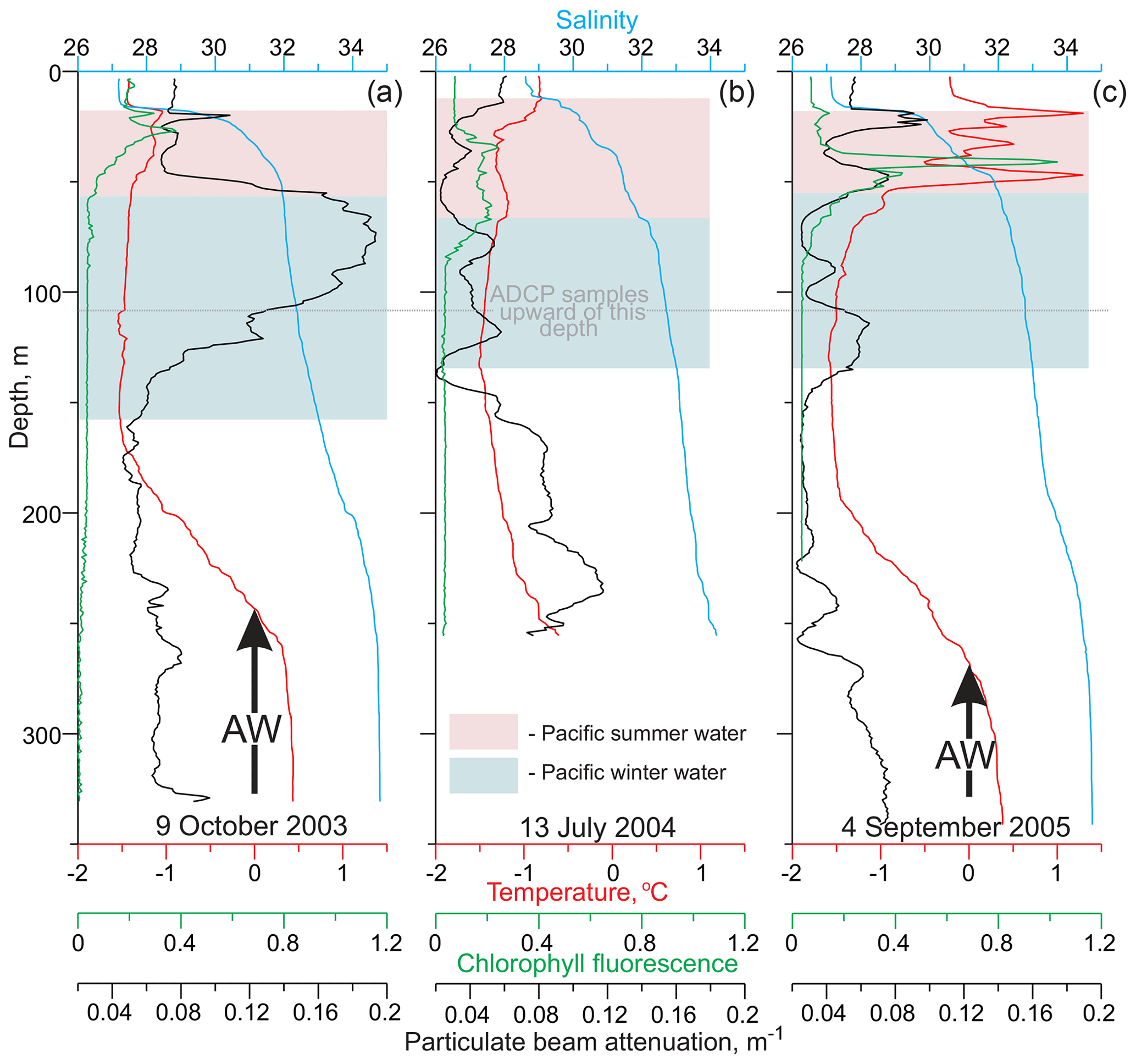
Figure 2Vertical temperature (red), salinity (blue), chlorophyll fluorescence (green), and particulate beam attenuation (black) profiles taken at (a) mooring deployment on 9 October 2003, (b) on 13 July 2004, and (c) at mooring recovery on 4 September 2005. Pink and blue shading and black arrows highlight Pacific Summer Water (PSW), Pacific Winter Water (PWW), and Atlantic Water (AW), respectively, following Dmitrenko et al. (2016).
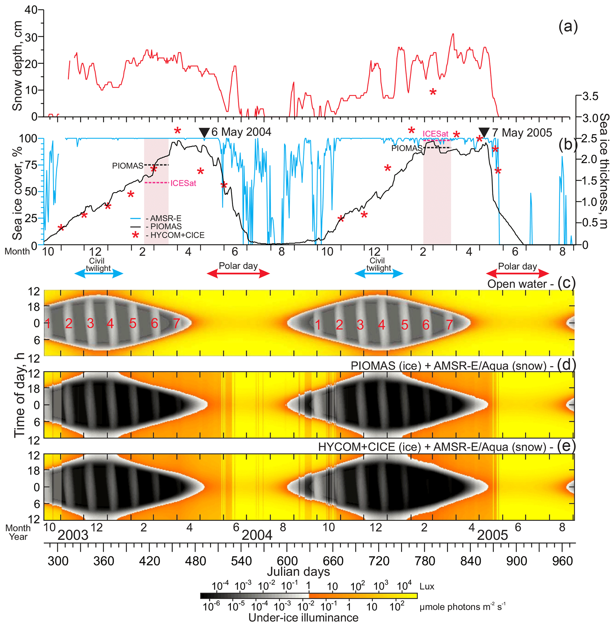
Figure 3Time series of the (a) snow depth (cm, red) as well as (b) sea-ice concentrations (%, blue) and thickness (m) from PIOMAS (black) and HYCOM+CICE (red stars). (b) Pink shading highlights periods of two ICESat campaigns. Black and purple horizontal segments indicate the mean sea-ice thickness derived from PIOMAS and ICESat, respectively. Black triangles at the top identify the time when the RADARSAT satellite images in Fig. 6 were acquired. (c–e) Actograms of under-ice illuminance modeled for (c) open-water conditions, (d, e) snow from AMSR-E/Aqua, and sea-ice thickness from (d) PIOMAS and (e) HYCOM+CICE. Red and blue arrows at the top indicate the polar day and civil twilight, respectively. (c) Red numbers reference the full moon occurrences.
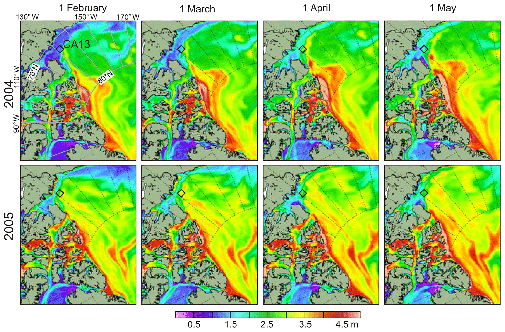
Figure 4Spatial distribution of sea-ice thickness (m) based on model simulations using DMI's ocean and sea-ice model HYCOM+CICE for February–May 2004 (top) and 2005 (bottom). The black diamonds depict the mooring position.
(iv) We also used data on sea-ice thickness from ICESat obtained from the NASA National Snow and Ice Data Center – NSIDS (Yi and Zwally, 2009). Data represent the gridded 25 km means. Kwok et al. (2007) found a mean uncertainty of the sea-ice thickness of about 0.7 m, and the sea-ice draft estimated from ICESat data relative to that measured at moorings agreed within 0.5 m. We use data from the ICESat campaigns previously used by Kwok et al. (2009): ON03 (24 September–18 November 2003), FM04 (17 February–21 March 2004), ON04 (3 October–8 November 2004), and FM05 (17 February–24 March 2005), shown in Fig. 5. Finally, we used (v) satellite synthetic aperture radar (SAR) imagery acquired by Canadian RADARSAT over the mooring location before the sea-ice breakup in 2004 and 2005 (Fig. 6a–d). RADARSAT data were acquired through the Government of Canada's Earth Observation Data Management System (https://www.eodms-sgdot.nrcan-rncan.gc.ca, last access: 20 October 2020).
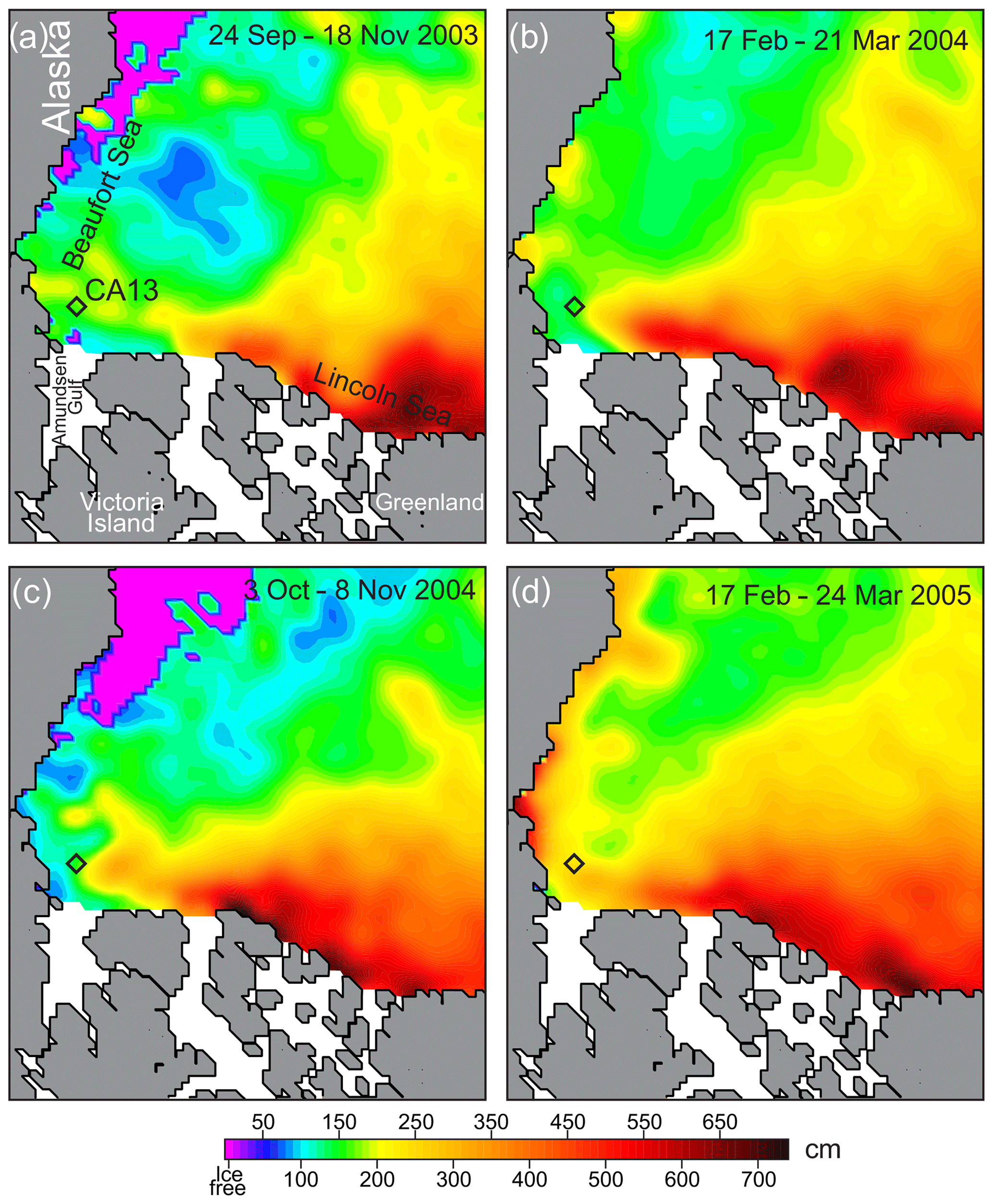
Figure 5Spatial distribution of sea-ice thickness (cm) over the Canada Basin compiled using gridded sea-ice thickness data from ICESat campaigns for (a) 24 September–18 November 2003, (b) 17 February–21 March 2004, (c) 3 October–8 November 2004, and (d) 17 February–24 March 2005 following Kwok et al. (2009). The black diamonds depict the mooring position.
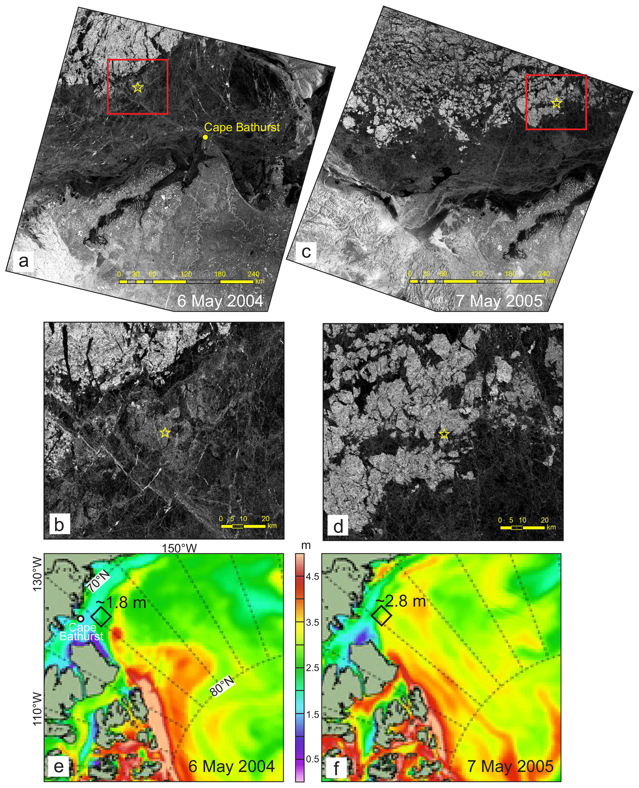
Figure 6(a–d) RADARSAT satellite images taken before sea-ice breakup over the CA13 location northeast of Cape Bathurst on (a) 6 May 2004 and (c) 7 May 2005. Red rectangles show the mooring region enlarged in (b) and (d). Yellow stars depict the mooring position. The dark areas are associated with the first-year pack ice (<2 m thick). The lighter areas indicate the multiyear pack ice (>2 m thick). (e–f) Spatial distribution of sea-ice thickness (m) based on the HYCOM+CICE model simulations for (e) 6 May 2004 and (f) 7 May 2005. The black diamonds depict the mooring position. Numbers show approximate sea-ice thickness.
Snow depth over sea ice, derived from AMSR-E/Aqua, was obtained from NSIDC (Cavalieri et al., 2014). The 12.5 km snow depth is provided as a 5 d running average. It is generated using the AMSR-E snow-depth-on-sea-ice algorithm based on the spectral gradient ratio of the 18.7 and 36.5 GHz vertical polarization channels (Markus and Cavalieri, 1998). As for the AMSR-E sea-ice concentrations, to generate time series of the snow depth over sea ice (Fig. 3a) we used data from the pixel closest to the mooring position.
We analyzed the acoustic backscatter and velocity time series from the ADCP to reveal modifications of the acoustic backscatter diurnal signal primarily dominated by DVM. In general, the particles in the water column producing a significant portion of acoustic backscatter comprise suspended sediments or planktonic organisms (e.g., Petrusevich et al., 2020). Frazil ice crystals also generate an enhanced acoustic backscatter (e.g., Dmitrenko et al., 2010). However, sound scattering produced by zooplankton is more complex compared to that generated by sediment particles due to DVM (Stanton et al., 1994). Moreover, ADCPs, unlike echo sounders, are limited in deriving accurate quantitative estimates of zooplankton biomass (Lemon et al., 2001, 2012; Vestheim et al., 2014). This is mainly due to calibration issues (Brierley et al., 1998; Fielding et al., 2004; Lemon et al., 2008; Lorke et al., 2004) and the beam geometry (Vestheim et al., 2014). To account for the beam geometry, we derived mean volume backscatter strength (MVBS) in decibels (dB) from the acoustic backscatter echo intensity following the procedure described by Deines (1999).
Using vertical velocity for DVM interpretation is not intuitive. The vertical velocity component is very sensitive to spatial inhomogeneity of the flow field and errors in the ADCP tilt angle, introducing errors and significant contamination to the measured vertical velocity component (Ott, 2005). Deviations of the vertical velocity diurnal pattern can also be attributed to a more dynamical (turbulent) state of the environment associated with high-velocity currents. In what follows, we are only interested in the vertical velocity estimates, which are sensitive to the MVBS diurnal cycling. For this analysis, the vertical velocity time series were filtered as follows. We removed diurnal cycling and low-frequency variability using a 24 h and 90 d running mean, respectively. All velocity values exceeding 1 standard deviation of the mean for the residual time series are considered noise attributed to spatial inhomogeneity of the flow field and errors in the ADCP tilt angle. In what follows, we show that the contaminated vertical velocity data are assigned to upwellings, downwellings, and eddies. Thus, they cannot be used for interpretation of DVM modifications imposed by these major high-velocity events. Therefore, our analysis of the impact of the major energetic events on DVM is entirely based on the vertical redistribution of the acoustic backscatter.
Under-ice illumination was modeled using the exponential decay radiative transfer model (Grenfell and Maykut, 1977; Perovich, 1996). Figure 3c shows the sea-surface illuminance at the mooring position computed for open-water conditions (no sea ice or snow cover). Transmittance through the sea ice and snow cover to depth z in the ice was calculated using the following equation: , where i0 is the fraction of the wavelength-integrated incident irradiance transmitted through the top 0.1 m of the surface layer, and Kt is the total extinction coefficient in the snow or sea-ice cover. The values adopted for the sea-ice and snow cover were i0=0.63 and Kt=1.5 as well as i0=50.9 and Kt=0.1, respectively (Grenfell and Maykut, 1977). For computing under-ice illumination in Fig. 3d and e, we use PIOMAS and HYCOM+CICE data on the simulated sea-ice thickness, respectively. The snow thickness on the top of the ice was taken from AMSR-E/Aqua observations. We accounted for the sea ice and snow cover if the sea-ice concentration exceeds 90 %. Cloud cover information was not utilized by this model taking due to high uncertainty of the cloud cover data (Liu and Key, 2016).
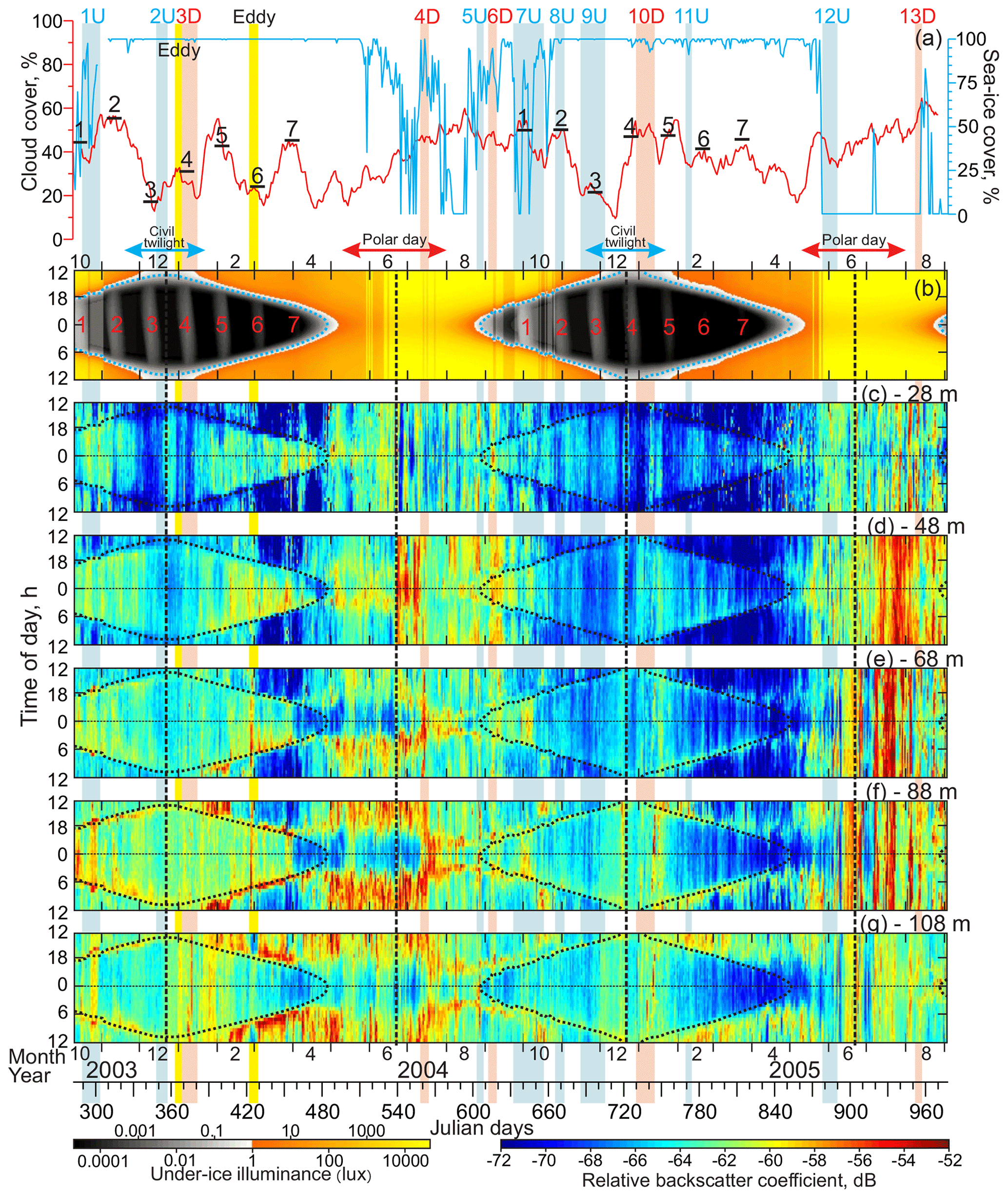
Figure 7(a) Time series of sea-ice concentrations (blue, %) and 15 d running mean of total cloud cover (red, %). Actograms of (b) modeled under-ice illuminance (lux) based on HYCOM+CICE sea-ice thickness and (c–g) MVBS (dB) at five depth levels: (c) 28, (d) 48, (e) 68, (f) 88, and (g) 108 m. The dotted blue (b) and black (c–g) lines depicts the 0.1 lux threshold. Red and blue arrows at the top indicate the polar day and civil twilight, respectively. Red numbers reference the full moon occurrences, and black horizontal segments in (a) indicate the mean cloud cover for these periods. Black dashed vertical lines depict solstices. Red and blue shading highlight the downwelling (D) and upwelling (U) events, respectively, with their reference numbers on the top. Yellow shading highlights eddies.
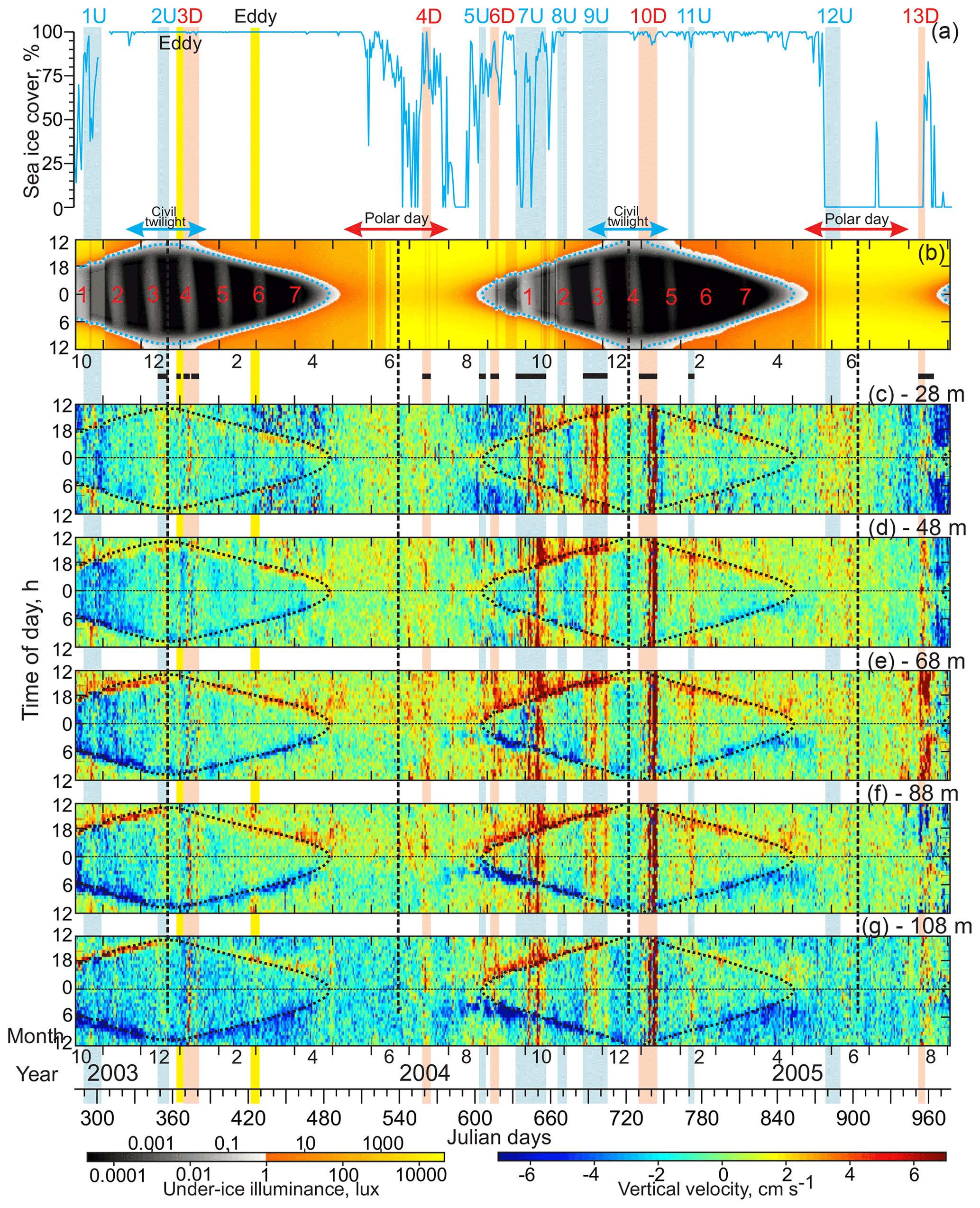
Figure 8(a) Time series of sea-ice concentrations (%). Actograms of (b) modeled under-ice illuminance (lux) based on HYCOM+CICE sea-ice thickness and (c–g) ADCP-measured vertical velocity (cm s−1) at five depth levels: (c) 28, (d) 48, (e) 68, (f) 88, and (g) 108 m. Positive–negative values correspond to the upward–downward flow. Horizontal black lines at the top of panel (c) depict periods of noise in vertical velocity attributed to spatial inhomogeneity of the flow field and errors in the ADCP tilt angle (for more details, see Sect. 3). All other designations are similar to those in Fig. 7.
Time series of MVBS (Fig. 7c–g), the vertical velocity component (Fig. 8c–g), and surface layer illumination (Figs. 7b and 8b), computed for the HYCOM+CICE sea-ice thickness, are presented in the form of actograms showing a rhythm of activity. Variations during a day-long period are presented along the vertical axis of the actogram, while the long-term patterns of diurnal behavior can be assessed following the horizontal axis (e. g., Leise et al., 2013; Last et al., 2016; Hobbs et al., 2018). For the actograms of illuminance we introduced an artificial visual boundary on the illuminance color scheme at 1 lux (gray to orange), which is the threshold that corresponds to illuminance during the deep twilight.
Following Barber et al. (2015), we used the kinetic energy, E= , derived from the zonal (U) and meridional (V) components of the current velocity to identify the major energetic events exceeding the 2 standard deviation threshold of ∼500 cm2 s−2. Using this threshold, Dmitrenko et al. (2018) identified 13 major energetic events comprised of upwellings and downwellings. They are highlighted in Figs. 7–9 with blue and pink shading, respectively.
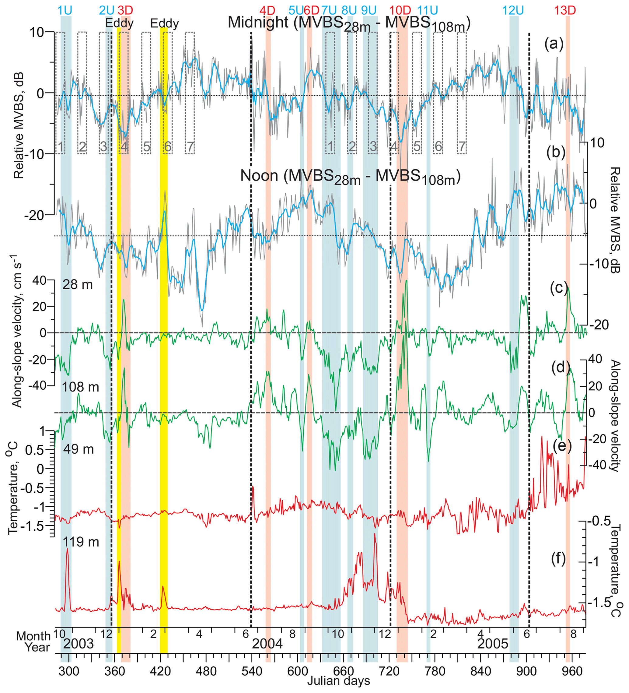
Figure 9Time series of the daily mean relative MVBS (dB) from 28 to 108 m of depth for the astronomic (a) midnight and (b) noon ±1 h, along-slope (positive northeastward) velocity for depths of (c) 28 and (d) 108 m (cm s−1) and water temperatures (∘C) for (e) 49 and (f) 119 m of depth. (a–b) Blue lines show the 7 d running mean. Horizontal dotted lines show the 2-year means. Positive–negative values correspond to MVBS gain and loss at 28 and 108 m of depth. (a) Gray dashed rectangles depict the full moon occurrence ±6 d. All other designations are similar to those in Fig. 7.
4.1 Sea ice
The southern Beaufort Sea is seasonally ice-covered. It is dominated by the first-year pack ice, with thickness gradually increasing from zero in September to ∼80–90 cm in March–April (Melling et al., 2005). In the Canada Basin beyond the eastern Beaufort Sea continental slope, ice conditions are partly dominated by the multiyear pack ice, with a mean thickness increasing from about 30 cm in August–September to 210–220 cm in May (Krishfield et al., 2014). The multiyear Greenland pack ice (>7 m thick) occupies the area to the north of the Canadian Arctic Archipelago and Greenland (e.g., Kwok et al., 2009).
On-slope displacement of the multiyear pack ice from the Greenland and Ellesmere Island shelves was observed during winter 2005. This is evident from the sea-ice thickness ICESat data showing a west–southward expansion of the Greenland pack in February–March 2005 (Fig. 5d). This is in line with detecting multiyear ice on the RADARSAT satellite imagery acquired over the mooring position in May 2005 (Fig. 6). The lighter areas in Fig. 6c and d indicate that the multiyear pack ice expanded over the mooring position before the sea-ice breakup in May 2005.
The satellite information on sea-ice thickness, however, is not consistent with PIOMAS. For February–March 2004 and 2005, PIOMAS provides estimates of sea-ice thickness at the mooring position of 1.87 and 2.28 m, respectively (Fig. 3b). In contrast, for the same time period, ICESat provides 1.5–1.4 and 2.4–2.5 m, respectively (Fig. 5c and d). This discrepancy is in line with the conclusions by Wang et al. (2016) that PIOMAS overestimates thicknesses for the thin ice area around the Beaufort Sea and underestimates the thick ice area around northern Greenland and the Canadian Arctic Archipelago. For winter–spring 2003–2004, PIOMAS data agree relatively well with HYCOM+CICE data (Fig. 3b). For January–May 2005, however, the discrepancy between PIOMAS and HYCOM+CICE increases from ∼0.5 m on 1 January to ∼1.3 m on 22 May 2005 (Fig. 3b). During winter–spring 2005, the spatial distribution of sea-ice thickness, derived from HYCOM+CICE simulations, shows the on-slope displacement of the multiyear pack ice from the Greenland and Ellesmere Island shelves (Fig. 4), which is also revealed from the satellite observations (Figs. 5 and 6a–d). For winter–spring 2005, the HYCOM+CICE data on the multiyear pack ice >2 m thick over the mooring position are in line with detecting multiyear ice on the RADARSAT satellite imagery acquired before sea-ice breakup in May 2005 (Fig. 6). Overall, the HYCOM+CICE simulations and satellite data suggest that during winter–spring 2005 sea-ice thickness over the mooring location exceeded that for 2004 by ∼1 m, with important implications for the under-ice illuminance values as evident from actograms of under-ice illuminance in Fig. 3d and e. In what follows, we use under-ice illuminance derived using the HYCOM+CICE simulations.
4.2 Temperature and salinity
The structure of the near-surface and intermediate water layers over the eastern Beaufort Sea upper continental slope, resolved by an ADCP, is comprised of a mixture of river runoff and sea-ice meltwater and seawater of Pacific origin (Fig. 2). A surface layer of relatively warm and low-salinity water (∼27–29) is freshened by the Mackenzie River runoff and sea-ice melt. Water with the salinity 29<S<33 is generally assigned to Pacific Water (PW) – e.g., Dmitrenko et al. (2016). It is transported along the Beaufort Sea continental slope by an Alaskan branch of the PW flow emanating from the Bering Strait. The relatively fresh PW layer impacts the halocline structure, producing a double halocline layer with low-stratified upper halocline water formed by the insertion of PW that overlies lower halocline water originating from the Eurasian Basin. In this study, we associated PW with the broad temperature range between 1.5 and −1.5 ∘C approximately centered at S ∼32 where the upper and lower halocline layers reside (Fig. 2). Pacific Summer Water (PSW) is broadly classified here as T>−1.2 ∘C and 30<S<32 (pink shading in Fig. 2). In October 2003, July 2004, and September 2005, PSW occupied the upper intermediate water layer from ∼25 to ∼60 m of depth (Fig. 2). This water mass is usually comprised of Chukchi summer water transported through Herald Canyon on the western Chukchi shelf (Woodgate et al., 2005) and Alaskan coastal water transported by the Alaskan coastal current through Barrow Canyon (Pickart et al., 2005). The underlying Pacific Winter Water (PWW), with a broad temperature minimum below −1.2 ∘C centered at S∼33 (blue shading in Fig. 2), is generated during freezing and brine rejection in the Bering and Chukchi seas (Weingartner et al., 1998; Pickart, 2004). During 2003–2005, PWW occupied the lower intermediate water layer at ∼60–140 m of depth (Fig. 2). The warm and saltier Atlantic Water, with temperatures above 0 ∘C and S>33.5, underlies PWW at depths >230 m, which significantly exceeds the depth range resolved with ADCP measurements (Fig. 2).
4.3 Water dynamics
The kinetic energy of currents over the eastern Beaufort Sea continental slope is mainly affected by the along-slope current component (Kulikov et al., 1998; Williams et al., 2006; Dmitrenko et al., 2016, 2018). For CA13, the maximum variability of currents is also consistent with the along-slope direction, explaining ∼70 % of the total velocity variability (Dmitrenko et al., 2018). Thus, major energetic events highlighted in Figs. 7–9 are primarily associated with along-slope flow dynamics, as also follows from the velocity time series in Fig. 9c and d. Among 13 major energetic events in Figs. 7–9, four events were clearly attributed to the depth-intensified flow (nos. 3D, 4D, 6D, and 10D; pink shading in Figs. 7–9) generated by ocean downwelling superimposed on the background bottom-intensified eastward shelf-break flow. Six events are associated with the surface-intensified or barotropic flow (nos. 1U, 2U, 7U, 8U, 9U, and 12U; blue shading in Figs. 7–9). These events were attributed to ocean upwelling (Dmitrenko et al., 2018). While events 5U and 11U are depth-intensified, they are highlighted with blue shading because they are consistent with upwelling-favorable atmospheric forcing that usually drives the surface-intensified events. In contrast, event 13D is surface-intensified, but it has been highlighted with pink shading because it is consistent with downwelling-favorable atmospheric forcing (Dmitrenko et al., 2018).
MVBS and vertical velocity actograms were computed for the depths of 28, 48, 68, 88 and 108 m (Figs. 7c–g and 8c–g). These actograms reveal a rhythm of activity with a diurnal cycle seen in the vertical axis of an actogram. The 2-year-long variability of the diurnal cycle is observed along the horizontal axis.
5.1 Seasonal patterns
In general, MVBS actograms resemble the seasonal variability of the diurnal signal following light conditions (Figs. 7b–g and 8b–g). In the subsurface layer (28 m of depth), a low MVBS corresponds to a relatively high illuminance during the day, while an elevated MVBS is consistent with a low illuminance during the night (Fig. 7b and c). In contrast, at 108 m of depth, MVBS shows an opposite pattern with a high MVBS during the light time of the day and a low MVBS in the darkness (Fig. 7b and g). This variability in MVBS is consistent with DVM.
In general, the MVBS diurnal signal follows the seasonal variability of the Sun illuminance during the entire year except for the period of the polar day when the diurnal pattern becomes significantly disrupted in the subsurface water layer. Outside of the polar day, the diurnal changes in the Sun illuminance are opposite to MVBS for the subsurface layer, while at 108 m of depth this relationship becomes positive. During the polar day, in the subsurface layer the MVBS diurnal rhythm vanishes (Fig. 7c). In spring 2004, the vanishing of the MVBS diurnal pattern from the beginning of May corresponds to an increase in the midnight under-ice illuminance to >0.1 lux (Fig. 7b and c). This modification lagged behind the sea-ice retreat off the mooring location by about 1 month (Fig. 7a and c). In contrast, during spring 2005, significant deviation of the MVBS diurnal rhythm was delayed by about 3 weeks compared to 2004. The deviation of the MVBS diurnal pattern was recorded once the sea ice disappeared from the mooring location on 20 May 2005. Note that the satellite-derived data and HYCOM+CICE simulations for winter–spring 2005 show that the sea-ice thickness over the mooring location exceeding that for 2004 by ∼1 m (Figs. 4–6). In spring 2005, the midnight under-ice illuminance >1 lux was lagging that in 2004 by about 1 week (Fig. 7b).
For the PW layer, the behavior of the MVBS diurnal signal during the polar day is different from the subsurface water layer. From about 1 April to 10 July 2004, the diurnal amplitude of the MVBS signal was enhanced at the 68–108 m depth layer due to MVBS values lowered from to −66 dB during the astronomic midnight ±3 h (Fig. 7e–g). In contrast to the preceding and subsequent periods, no seasonal modulation of the MVBS diurnal cycle was observed at this time. This is in line with illuminance, showing almost no seasonal modulation during the midnight sun (Fig. 7b). For the polar day period in 2005, however, enhancement of the MVBS diurnal signal seemed to be impacted by short-term high-MVBS events likely generated by intrusions of turbid water. These events were found to be most pronounced through the PSW layer where intrusions of turbid and relatively warmer water were observed during mooring recovery (Figs. 2c, 7d, and e).
Following the midnight sun, the MVBS diurnal signal returned once the mooring position became 100 % ice-covered from 7 November 2003 and 25 October 2004 (Fig. 7a and c–g). This is evident from enhancing the MVBS difference between the light (>1 lux) and dark (<1 lux) time for 28–48 m of depth (Fig. 7c–d). The noticeable feature of the MVBS diurnal signal during civil twilight and the subsequent period until the end of April is a significant MVBS difference between 2003–2004 and 2004–2005 observed during the dark time through the entire water column resolved with ADCP observations (Fig. 7c–f). Another noticeable feature of MVBS during this period is numerous disruptions of the diurnal signal, discussed below in Sect. 5.3.1 and 5.3.2.
Behind the seasonality of the diurnal signal in the MVBS time series, the seasonal cycling of the MVBS vertical distribution has been revealed (Fig. 9a and b). For midnight, during low-light conditions from October to February (civil twilight length exceeds daylight length), MVBS tends to increase with depth from 28 to 108 m (Fig. 9a). In March–June, the midnight MVBS shows an opposite tendency (Fig. 9a). The MVBS midnight long-term mean, however, shows almost no difference from 28 to 108 m of depth, with a long-term mean of −0.6 dB. The seasonal cycle of the MVBS vertical distribution for the astronomic noon is different. From about the winter to the summer solstice, MVBS at 128 m of depth exceeds that for 28 m of depth by about 8 dB (Fig. 9b). In contrast, during the ice-free period in June-August, the MVBS difference from 28 to 108 m of depth tends to decrease down to about zero in late summer. The long-term mean for the astronomic noon (−5.3 dB; Fig. 9b) shows a general tendency of MVBS to increase with depth.
The vertical velocity actograms also show a diurnal pattern around astronomic midnight (Fig. 8c–g) that is consistent with the MVBS diurnal rhythm in Fig. 7c–g. Net upward movement is regularly observed before the astronomic midnight once the under-ice dark-time illuminance is <0.1 lux (Fig. 8b–g). Moreover, the most intense upward flow was recorded during 1–3 h after the illuminance dropped below the 0.1 lux threshold. In contrast, a downward net flow was recorded following the tendency of under-ice illuminance to increase from midnight to noon once illuminance exceeded the 0.1 lux threshold (Fig. 8b–g). At the end of April 2004, once under-ice illuminance exceeded the 0.1 lux threshold 24 h a day approaching the midnight sun, the vertical velocity diurnal signal completely vanished. During May–June 2004, however, a weaker net upward and downward diurnal movement of about ±0.5 cm s−1 was recorded at 68 and 88 m of depth from noon to midnight (light blue to green shading in Fig. 8e and f) and from midnight to noon (light green to yellow shading in Fig. 8e and f), respectively. This is consistent with the MVBS diurnal rhythm revealed through the PW layer during summer 2004 (Fig. 7e–g). Following the under-ice illuminance, a pronounced velocity diurnal signal again appeared at the end of August 2004 when the midnight under-ice illuminance decreased to the 0.1 lux threshold, gradually returning to civil twilight. In spring 2005, the vertical velocity diurnal signal was relatively well pronounced until the midnight under-ice illuminance was below the 0.1 lux threshold (Fig. 8b–g). As for MVBS, complete cessation of a diurnal signal in vertical velocity in spring 2005 was observed at 68–88 m of depth only when sea ice started to retreat in mid-May (Fig. 8a). In this case, complete cessation of the diurnal signal lagged behind the 0.1 lux threshold by about 20 d (Fig. 8b, e, and f). During the midnight sun 2005, the velocity diurnal rhythm is unrecognizable.
Finally, the velocity diurnal signal varies with depth. The upward and downward flow attributed to diurnal cycling is higher and less noisy at 68–88 m of depth compared to the overlaying subsurface layer at 28–48 m of depth and to a lesser extent to the underlying water at 108 m of depth (Fig. 8c–g).
5.2 Moon cycle
During the period of civil twilight when the Sun is more than 6∘ below the horizon, moonlight is the main source of illumination over the eastern Beaufort Sea continental slope (Fig. 7b). The full moon has a mean period of 29.53059 d called a synodic or lunar month. During midwinter (end of December), the full moon generates under-ice illuminance up to about 0.001 lux below the sea-ice layer with a thickness of around 1 m and ∼20 cm snow depth over sea ice (Figs. 3b and 7b). In contrast, for open-water conditions, the full moon generates illuminance exceeding 0.1 lux (Fig. 3c). Sea ice strongly attenuates moonlight. Once sea-ice thickness exceeded ∼2.5 m in April 2004 and February 2005, moonlight transmittance through sea ice was completely terminated (Fig. 3b and e). While the cloud cover attenuates moon illumination, it was not considered for modeling under-ice illuminance due to high uncertainty of the cloud cover data (Liu and Key, 2016).
The MVBS diurnal signal is impacted by moonlight and also attenuated by the cloud cover. Once the full moon (±6 d) occurred during the period of civil twilight, the cloud cover showed three low-cloud events with cloud cover ≤30 % (nos. 3 and 4 in 2003–2004 and no. 3 in 2004–2005 in Fig. 7a and b). During these events, the MVBS diurnal signal was significantly disrupted in the subsurface layer, and a low MVBS was observed during the entire 24 h (Fig. 7b and 7c). For full moon event no. 4 in January 2004, during the astronomic midnight, a low MVBS at 28 m of depth was associated with an elevated MVBS at 108 m of depth, as evident from decreasing the MVBS difference from 28 to 108 m of depth in Fig. 9a. Overall, among 14 full moon events that occurred in October–March 2003–2004 and 2004–2005 once the midnight under-ice illuminance was <1 lux, three events in February–March (no. 7 in 2004 and nos. 6 and 7 in 2005) show complete cessation of moonlight transmittance through sea ice exceeding 2.5 m thick (Fig. 7b). Events 1–5 in 2003–2004 and 1, 2, and 5 in 2004–2005 demonstrated similar anomalies of the MVBS difference from 28 to 108 m of depth (Fig. 9a). During noon, however, this pattern is not obvious (Fig. 9b).
Full moon event no. 1 in September–October 2004 gives an example of the moonlight impact on the MVBS diurnal signal (Fig. 7). While the cloud cover during this event was relatively high (∼50 %, Fig. 7a), the dark-time MVBS dropped by ∼2 dB at 28 m of depth but elevated by ∼4 dB at 68 and 88 m of depth, suggesting the downward displacement of acoustic backscatter (Fig. 7c and f–g, respectively). At noon, however, MVBS elevated by ∼4 dB at 28 m of depth (Fig. 7c). Note that during this time the under-ice illuminance was reduced as the mooring became ice-covered (Fig. 7a). It is also important to point out that this full moon event partly overlaps upwelling 7U described below.
5.3 Short-term oceanographic events
The regular diurnal pattern of MVBS was disrupted during short-term events lasting from several days to several weeks (Fig. 7c–g). These events also interplay with disruptions generated by moon cycling. We use actograms of vertical velocity to differentiate disruptions imposed by moonlight from those of dynamic origin (Fig. 8c–g). In general, the diurnal pattern remains recognizable during the full moon events (Fig. 8b–g). In contrast, almost all significant or even complete short-term disruptions of the vertical velocity diurnal rhythm are related to upwelling or downwelling (Fig. 8c–g).
Dmitrenko et al. (2018) identified upwelling or downwelling events at CA13 using ADCP velocity data, the NCEP-derived wind and sea-level atmospheric data, sea-surface height records at Tuktoyaktuk (Fig. 1), and numerical simulations. All these events are highlighted in Figs. 7–9 with blue and red shading for upwelling and downwelling, respectively.
5.3.1 Upwelling events
Upwelling events disrupt the MVBS diurnal signal in a similar way as moonlight does. For upwelling 1U, MVBS at 108 m of depth was elevated throughout the full 24 h period (Fig. 7g). During the dark time (illuminance <1 lux) at 28 m of depth, MVBS was reduced to the end of the event when the surface-intensified flow at 28 m of depth shows maximum velocities exceeding 30 cm s−1 (Fig. 9c). Moreover, upwelling 1U resulted in ∼0.7 ∘C temperature increase at 119 m of depth (Fig. 9f). Upwelling 2U occurred right before the winter solstice and shows significant MVBS reduction at 28–48 m of depth, gradually vanishing to 108 m of depth. Upwelling 5U occurred at the end of the ice-free season and shortly after the end of the midnight sun 2004. Therefore, the MVBS diurnal signal was relatively weak and noisy, especially at 28 m of depth. However, MVBS increase at 88–108 m of depth is likely attributed to upwelling. Upwelling 7U interplayed with full moon event no. 1 in September–October 2004. It seems that the first portion of this event until 3 October 2004 was dominated by moonlight. Afterward, once the horizontal velocity at 28 m of depth exceeded ∼30 cm s−1 (Fig. 9c), a slight reduction of MVBS is observed at 28–48 m of depth during the dark time. In contrast to the preceding upwelling events, no elevated MVBS values were recorded in the overlying water layer. Upwelling 8U completely coincided with full moon event no. 2 in October–November 2004. As with the majority of the full moon and upwelling events, it shows the downward redistribution of acoustic backscatter from 28–48 m to the deeper water layer (Figs. 7c–g, 9a, and 9b). A similar overlap between the full moon and upwelling was observed during upwelling 9U. Significant MVBS reduction within 28–48 m was accompanied by elevated MVBS at 88–108 m of depth during the latter part of this upwelling from 25 November to 5 December 2004. Overall, upwelling event nos. 7–9 resulted in a gradual increase in temperature at 119 m of depth from −1.55 to −0.65 ∘C (Fig. 9f). Upwelling 11U shows an elevated MVBS during the light time at 88–108 m (Figs. 7f, g, and 9b). However, no significant modifications of the MVBS diurnal signal were observed in the overlying water. The last upwelling 12U in May–June 2005 occurred during the midnight sun when the MVBS diurnal signal mostly vanished, and MVBS is noisy. We speculate that this noise is due to the enhanced concentration of suspended particles in the water column (Fig. 2c).
Overall, among eight upwelling events observed in 2003–2005, six events (nos. 1, 2, 5, 7, 8, 9U) clearly show the MVBS reduction in the subsurface water layer at 28 m of depth (Fig. 7c). For upwellings 1, 5, 7, and 8U the midnight MVBS difference from 28 to 108 m of depth tends to decrease, which is consistent with a downward redistribution of acoustic scatter (Fig. 9a). This effect is similar to the MVBS response to the full moon events as described in Sect. 5.2. It seems that the overlap between upwelling and the full moon can dominate the MVBS response to upwellings 7–9U (Fig. 7b–g). During the polar day, the MVBS diurnal signal is weak or completely disrupted, and its response to upwelling is barely traceable (upwelling 12; Fig. 7b–g). Finally, wind, forcing upwelling events, also impacts the sea-ice cover through off-shelf displacement of the pack ice as evident for upwelling event no. 12 in May–June 2005 (Fig. 7a).
5.3.2 Downwelling events
Downwelling events disrupt the MVBS diurnal signal in the opposite way compared to upwellings and moonlight, moving acoustic backscatter upwards. Downwelling also interferes with MVBS modifications imposed by sea ice and the MVBS diurnal signal deviations generated by moonlight. Wind, forcing downwelling events, also impacts the sea-ice cover through on-shelf displacement of the pack ice as evident for downwelling events 4, 6, and 13D (Fig. 7a). Deviations of the MVBS diurnal signal due to moon cycling interfere with those caused by downwelling event no. 3, complicating our analysis.
Downwelling 3D occurred at the end of 2003–2004 during civil twilight and strongly interfered with full moon event no. 4 (Fig. 7). It seems that event 3D is entirely dominated by the moon, disrupting the MVBS diurnal signal as described in Sect. 5.2. Downwelling 4D was recorded at the end of the polar day 2004 when the MVBS diurnal signal terminated at 28–88 m of depth (Fig. 7c–f). Wind, forcing downwelling 4D, displaced pack ice on-shelf, and the CA13 position was reoccupied by sea ice for about 10 d, with implications for under-ice illuminance. Figure 7c and d show that sea ice and downwelling did not impact MVBS at 28–48 m of depth. In contrast, the midnight-sun diurnal signal at 68–88 m of depth was disrupted due to elevating MVBS at 68–88 m of depth during the dark time (from 22 to 4 h, Fig. 7e and f). At the same time, the midnight-sun diurnal signal at 108 m of depth remained undisturbed (Fig. 7g). Downwelling 6D provides the most comprehensive example of how the MVBS diurnal signal is disrupted by downwelling. In contrast to the full moon and upwelling events, MVBS at 28–48 m of depth was enhanced 24 h a day (Fig. 7c and d), suggesting the upward redistribution of acoustic backscatter from the underlying water layer (Fig. 9a and b). Note that during this event water dynamics were dominated by along-slope depth-intensified flow increasing from ∼5 cm s−1 at 28 m of depth (Fig. 9c) to >30 cm s−1 at 108 m of depth (Fig. 9d). Downwelling 10D was recorded at the end of civil twilight 2004–2005. It appears that the beginning of this event is impacted by the full moon (no. 4, 2004–2005) with the reduction of MVBS in the subsurface layer at 28 m of depth. However, by the end of downwelling 10D, once the bottom-intensified flow exceeded 100 cm s−1 at 128 m (Fig. 9d), MVBS at 28–48 m of depth tended to increase, suggesting the upward redistribution of acoustic backscatter, similar to downwelling 6D. Downwelling 13D occurred in mid-August 2005 following the midnight sun. During this time, the MVBS diurnal signal at 28 m of depth was not traceable. At 48–88 m of depth, the midnight-sun diurnal signal was likely masked due to the enhanced concentration of suspended particles in the water column (Fig. 2c).
Overall, among five downwelling events recorded in 2003–2005, event 6D and partly 10D show disruption of the MVBS diurnal signal in the subsurface water layer, with MVBS elevated at 28–48 m of depth in response to downwelling. Downwelling events 4 and 13D occurred during and shortly after the midnight sun, respectively, when the subsurface MVBS diurnal signal vanishes. Downwelling event 3D was dominated by moonlight.
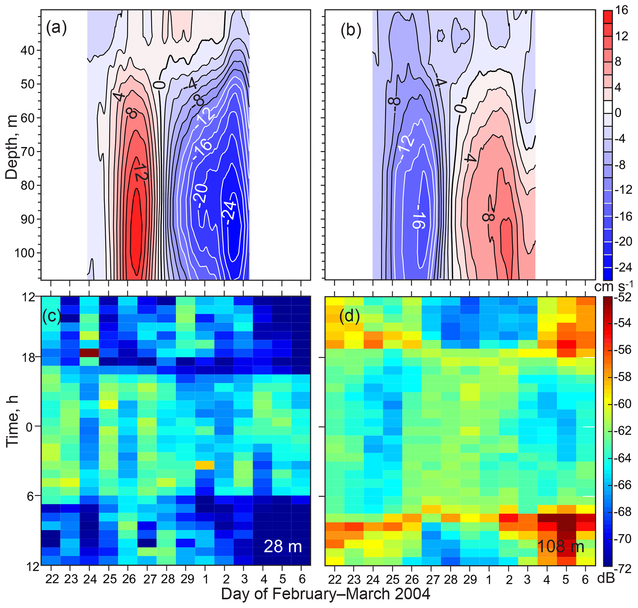
Figure 10Enlarged view of the February–March 2004 eddy. (a) Zonal and (b) meridional current (cm s−1) records as functions of depth adopted from Dmitrenko et al. (2018). (c–d) Actograms of MVBS (dB) for (c) 28 and (d) 108 m of depth.
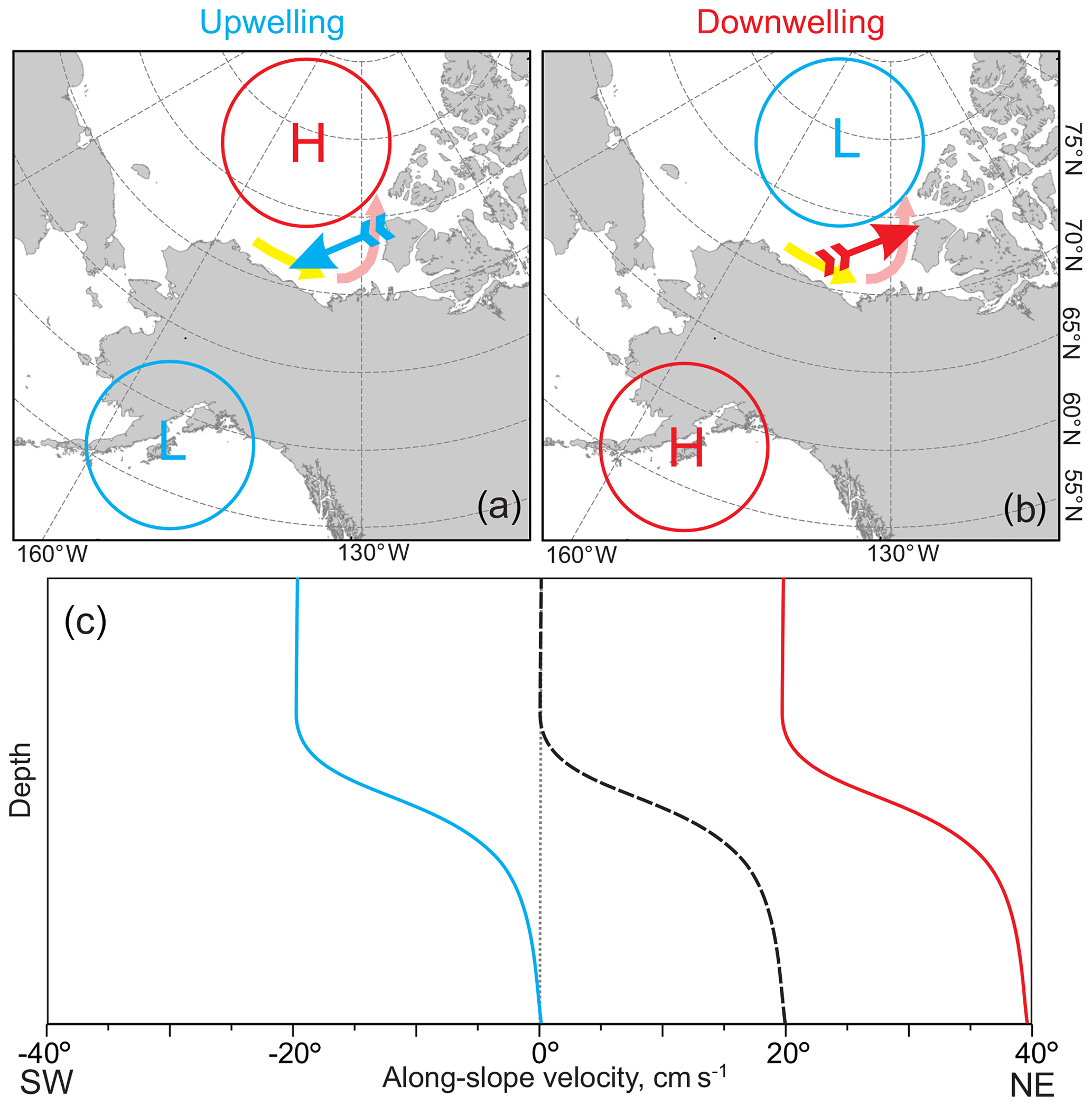
Figure 11Schematic depiction showing atmospheric forcing for (a) upwelling and (b) downwelling along the eastern Beaufort Sea continental slope adopted from Kirillov et al. (2016). Blue and red arrows indicate geostrophic wind associated with concurrence between the atmospheric low and high depicted by blue and red circles, respectively. Yellow and pink arrows show circulation with shelf-break jet over the western and eastern Beaufort Sea, respectively, intensified by local downwelling. (c) Schematic depiction suggesting the generation of surface-intensified (blue curve) and depth-intensified (red curve) along-slope currents as a result of upwelling and downwelling, respectively, superimposed on the hypothetical bottom-intensified shelf-break current (black dashed curve) following Dmitrenko et al. (2018).
5.3.3 Eddies
Eddies are ubiquitous over the Arctic Ocean continental slope (e.g., Dmitrenko et al., 2008; Pnyushkov et al., 2018), particularly over the Beaufort Sea continental slope (e.g., Spall et al., 2008; O'Brien et al., 2011). An eddy carrying entrained suspended particles was identified by Dmitrenko et al. (2018) based on ADCP velocity and acoustic backscatter time series in February–March 2004 (Figs. 7 and 10). One more eddy passed the mooring position in December–January 2003–2004 right before downwelling 3D. In Figs. 7–9 both eddies are highlighted with yellow shading.
The eddy in February–March 2004 provides an example of how the velocity field attributed to eddy passing disrupts the MVBS diurnal signal (Fig. 10). The greatest tangential speed, exceeding 22 cm s−1, marks the eddy core near 95 m of depth (Fig. 10a and b). Below the core at 119 m of depth, a positive temperature anomaly of 0.25 ∘C, attributed to the eddy passing, was recorded on 26 February 2004 (Fig. 9f). The velocity signature of the eddy is hardly discernible shallower than about 50 m, where the temperature anomaly does not exceed ∼0.1 ∘C (Figs. 9e, 10a, and b). During the dark time at 108 m of depth (below the depth of the greatest tangential speed), an enhanced MVBS was observed between two maxima of the eddy tangential speed from 27 February to 2 March 2004 (Fig. 10d). In contrast, during the daylight, a negative MVBS anomaly was recorded (Figs. 7g and 10d). This completely inverted the MVBS diurnal signal observed at 108 m of depth during the eddy passing. At 28–48 m of depth, however, MVBS was not significantly modified. Nevertheless, MVBS was slightly elevated during the light time (Figs. 7c, g and 10c). In contrast to water layers above and below the eddy core, from 26 February to 1 March the MVBS diurnal signal at 68–88 m of depth was disrupted by the backscatter maximum recorded for 24 h a day (Fig. 7e and f). It appears that this MVBS anomaly is attributed to the eddy-entrained suspended particles commonly recorded in this area (O'Brien et al., 2011).
The eddy in December–January 2003–2004 generated much less MVBS disturbance compared to the one in February–March 2004 (Fig. 7c–g). The core of the eddy was likely deeper than the ADCP transducer. A positive temperature anomaly at 119 m of depth was 0.5 ∘C (Fig. 9f). A positive MVBS anomaly was recorded only at 108 m of depth 24 h a day (Fig. 7g), likely indicating the eddy-entrained suspended particles. MVBS in the overlaying water layer was not significantly modified.
In summary, the eddy in February–March 2004 inverted the MVBS diurnal signal in the water layer below the eddy core defined by the greatest tangential speed of the horizontal flow. The eddy in December–January 2003–2004 generated no significant MVBS modifications as the eddy core was likely located below the ADCP.
The 2-year-long ADCP time series of MVBS and vertical velocity over the upper eastern Beaufort Sea continental slope are consistent with DVM of zooplankton. The MVBS diurnal signal is generated by a diurnal movement of zooplankton toward the surface at dusk and descent back the next morning before dawn. DVM demonstrates predator-avoidance behavior (Hays, 2003). Zooplankton keep away from a relatively well-illuminated surface water layer during the light time, reducing light-dependent mortality risk. The acoustic data from the single-frequency ADCP do not provide any information on the identity of organisms responsible for the observed DVM patterns, and proper studies on DVM have not been carried out in the Beaufort Sea prior to the present work. Thus, our analysis is significantly limited by the deficiency of zooplankton observations. Moreover, a comprehensive analysis of the scattering species comprising DVM is logistically impossible for long-term deployments in the seasonally ice-covered and remote areas of the high Arctic. This prohibits identification of specific species whose DVM was detected by the 300 kHz ADCP and altered by the different environmental factors, including illuminance and water dynamics. The deficiency of our analysis clearly shows a necessity to expand mooring observations using underwater electronic holographic cameras such as those described by Sun et al. (2007).
In general, DVM at CA13 is controlled by light conditions (Figs. 7 and 8). As for the other areas of the ocean, DVM is triggered by local solar variations, and the timing of migration is sensitive to changes in seasonal day length (e.g., van Haren and Compton, 2013). Our results show that DVM responds to (i) the seasonality of sunlight, (ii) the seasonality of sea-ice cover that attenuates light transmission to the water column, and to a lesser extent to (iii) moonlight. Moreover, (iv) DVM can be modified or completely disrupted during highly energetic current events generated by upwelling, downwelling, or eddy passing. Our results also suggest that the interplay between all these factors impacts DVM at CA13. Furthermore, MVBS is not entirely controlled by DVM. The suspended particles in the water column enhance acoustic scattering, impacting DVM during the midnight sun (Figs. 2a, and 7b, d, and e) and also attenuating light intensity in the water column. Below we discuss all these factors and their impact on DVM in more detail.
6.1 DVM seasonal cycle, sea-ice cover, and suspended particles
It appears that DVM is triggered once the estimated near-surface illuminance falls below the 0.1 lux threshold (Figs. 7 and 8). This suggests that the diurnal movement of zooplankton toward the surface at dusk starts once the near-surface illuminance decreases to ∼0.1 lux and descends back the next morning before dawn as soon as the near-surface illuminance exceeds 0.1 lux. DVM follows changes in seasonal day length, and it stops at the subsurface layer as soon as near-surface illuminance retains above ∼0.1 lux for 24 h a day (Fig. 7b–g). At the CA13 latitude (71∘21.356′ N), the estimated value of near-surface or under-ice illuminance exceeded the 0.1 lux threshold for about 55 and 50 d before the midnight sun in 2004 and 2005, respectively (Fig. 7b). During fall 2004, the subsurface DVM returned about 27 d after the polar day season, once the midnight near-surface illuminance dropped below the ∼0.1 lux threshold around 28 August (Fig. 7b–g). Our results on the light threshold are consistent with the preferendum (isolume) hypothesis (e.g., Cohen and Forward, 2009). A variant of the preferendum hypothesis, the absolute intensity threshold hypothesis, suggests that an ascent at sunset is initiated once the light intensity decreases below a particular threshold level, and a descent at sunrise occurs when the light intensity increases above the threshold intensity (e.g., Cohen and Forward, 2019). This is in line with our findings on an absolute 0.1 lux threshold of light, which corresponds to moonlight illuminance during the gibbous moon under a clear sky (Gaston et al., 2014).
The interannual variability in estimated under-ice illuminance is entirely attributed to the sea-ice thickness. During the ice season, the mean cloud cover (∼40 %) showed insignificant interannual variability (Fig. 7a); thus, the cloud cover was not taken into account. Our results reveal that sea-ice cover modifies the DVM seasonal cycle by attenuating under-ice illuminance. During winter–spring 2004, CA13 was primarily covered with first-year pack ice about 1.6 m thick (Figs. 3b, 4 top, 5a, and b). In contrast, during the same time in 2005, the eastern Beaufort Sea continental slope was occupied by multiyear pack ice about 2.6 m thick (Figs. 3b, 4 bottom, 5c, and d). We suggest that this increased sea-ice thickness extended the DVM seasonal cycle toward the polar day of 2005. In May 2005, the 0.1 lux threshold estimated for ∼2.5 m thick ice lagged behind that for 2004 by about 5 d (Fig. 7b). Following ice-diminished illuminance in April–May 2005, DVM at 28 m of depth was recorded until the beginning of May 2005. Moreover, DVM maintained integrity at 68–108 m of depth until the open-water season started in mid-May 2005 (Fig. 7a and e–g, respectively). In contrast, during spring 2004, DVM vanished about 12 and 28 d ahead of the polar day and open-water season, respectively (Fig. 7). We suggest that this interannual DVM variability is consistent with under-ice illuminance. Its estimated value for mid-May 2004 (≥10 lux) exceeds that for May 2005 by a factor of 10 (Fig. 7b).
The MVBS actograms show asymmetry of the DVM seasonal cycle to the summer solstice (Fig. 7b–g). In summer 2004, the DVM seasonal cycle terminated about 54 d before the summer solstice but resumed, lagging behind the summer solstice by 67 d. This asymmetry, being consistent with the estimated 0.1 lux threshold, is likely attributed to seasonal sea-ice cover. During spring, the polar day begins when the eastern Beaufort Sea continental slope is still ice-covered (Fig. 6), which governs attenuation of light below the ice. In contrast, after the polar day is ended, the eastern Beaufort Sea continental slope remains ice-free or partly ice-covered until the end of October, allowing sunlight to illuminate the near-surface water layer.
In the subsequent winters, the DVM backscatter intensity shows significant interannual variability. The dark-time MVBS during winter 2003–2004 exceeds that for winter 2004–2005 by ∼3–5 dB (Fig. 7c–g). We attribute this interannual variability to attenuation of light by a thicker ice cover in winter 2004–2005, as follows from our preceding discussion. Satellite data and model simulations show that the eastern Beaufort Sea continental slope was occupied by Greenland pack ice during winter–spring 2005 (Figs. 4–6), which results in a reduced estimate of under-ice illuminance by a factor of 10 (Fig. 7b). For example, during full moon event nos. 6 and 7 in February–March 2005, the nighttime moonlight illuminance decreased to the background nighttime illuminance of >0.0001 lux (Fig. 7b).
In general, our results on the sea-ice impact on DVM show that DVM is well synchronized with the light–dark cycle modified by sea-ice cover shading. It appears that thicker ice observed during winter 2004–2005 reduced the backscatter values (Fig. 7c–g), which likely demonstrates a light-mediated response of the zooplankton involved in DVM. This is in line with Berge et al. (2009) reporting a stronger polar night DVM in the ice-free Svalbard fjord compared to the ice-covered fjord. Vestheim et al. (2014) reported shallowing DVM in Oslofjord in response to freeze-up and subsequent snowfall. They attributed this shallowing to a relative reduction of light intensities, which is similar to that observed over the eastern Beaufort Sea continental slope during winter–spring 2005. La et al. (2015) suggested that sea ice diminishes DVM signals by blocking the detectable light intensity for DVM with depth during the Antarctic winter. At the same time, our results contrast with the observations of Wallace et al. (2010). They found no difference in the time of the DVM onset and cessation between the seasonally ice-covered and ice-free Svalbard fjords, insisting on the role of the relative change in irradiance for triggering DVM. This discrepancy highlights an important difference between sea ice in the Svalbard fjords and the eastern Beaufort Sea continental slope. Rijpfjorden in Svalbard is seasonally ice-covered with land-fast ice ∼0.8 m thick (Wallace et al., 2010). In contrast, in spring 2015 the eastern Beaufort Sea continental slope was occupied by 2.6 m thick multiyear Greenland pack ice (Figs. 3b, and 4–6), favoring synchronized DVM to extend toward the midnight sun.
Our data show that, during the midnight sun 2004, DVM ceased only at 28 m of depth. In the underlying PW layer at 48–108 m of depth, DVM continued until the beginning of July 2004 (Fig. 7c–g). However, DVM in the PW layer did not occur in phase with the 24 h light cycle. It seems that zooplankton were conducting regular synchronized DVM, but they were still avoiding relatively well-illuminated subsurface water. This is in line with predator-avoidance behavior during transitional seasons, but without seasonal modulation, because the Sun is above the horizon 24 h a day. In fact, zooplankton limit DVM to the PSW layer with relatively high chlorophyll fluorescence values during late summer (Fig. 2). This can indicate high concentrations of phytoplankton (e.g., La et al., 2018), which zooplankton feed on. The availability of phytoplankton can be an important factor triggering seasonal variability in DVM (e.g., La et al., 2015).
Usually, synchronized DVM stops during the midnight sun, consistent with predator-avoidance behavior of zooplankton conducting DVM (e.g., Blachowiak-Samolyk et al., 2006; Cottier et al., 2006; Wang et al., 2015; Darnis et al., 2017). However, Fortier et al. (2001) reported a clear midnight-sun DVM in copepods under the spring ice of Barrow Strait at the center of the Canadian Arctic Archipelago. They argued that absolute light intensity below sea ice decreases to the thresholds at which the feeding activity of fish slows down. Moreover, DVM below 2 m thick ice in the Canada Basin during the midnight sun was recently reported by La et al. (2018). Following Fortier et al. (2001), we speculate that the absolute light intensity through the PW layer at CA13 was below the threshold of predator perception, allowing DVM during the midnight sun 2004. However, the midnight-sun DVM was not obvious in 2005.
We suggest that the midnight-sun DVM in 2005 was likely impacted by the enhanced concentration of suspended particles through the PSW layer. Suspended particles return the ADCP signal, producing enhanced MVBS 24 h a day. For example, Petrusevich et al. (2020) reported enhanced MVBS in Hudson Bay recorded by a 300 kHz RDI Workhorse ADCP. They attributed this signal to the suspended particles released to the water column during ice melt. In contrast to vertically synchronized DVM, suspended particles generated noise that can mask DVM during the midnight sun 2005 as evident from Fig. 7d–f. On the CTD profile taken in September 2005, high particulate beam attenuation layers at around 25 and 50 m of depth match temperature maxima up to 1.3 ∘C (Fig. 2c). Moored CTD at 49 m of depth shows several maxima up to 0.5 ∘C following summer solstice 2005 (Fig. 9e). Two temperature maxima in early and middle June 2005 (Fig. 9e) match MVBS maxima at 68–88 m of depth (Fig. 7f and g). This suggests that MVBS maxima in actograms are generated by lateral advection of warm and turbid water layers. The formation of this water is likely attributed to wind-forced vertical mixing over the Beaufort Sea shelf involving surface riverine water heated by solar radiation and enriched with suspended particles. Alternatively, suspended particles can be attributed to resuspension of bottom sediments over the Beaufort Sea shelf. In any case, regardless of the source of suspended particles, their enhanced concentration in the water column during summer 2005 resulted in increased light attenuation (e.g., Hanelt et al., 2001), which potentially modified DVM during the midnight sun 2005.
6.2 DVM modifications by moonlight
In general, interpretation of DVM modifications due to moonlight is not straightforward. The dark-time MVBS in Fig. 7c shows the cumulative effect of sea ice, cloud cover, water dynamics, and moonlight. Individual events are often overlaid, and uncertainty in cloud cover also introduces an additional complication. Furthermore, during February–March, the moonlight below sea ice is strongly attenuated (2004) or completely absorbed by sea ice (2005) – Fig. 3e. Moreover, under-ice vertical velocity data do not show DVM disruptions during full moon phases (Fig. 8). However, MVBS actograms in Fig. 7c–g indicate modifications of DVM during a few days near the time of the full moon. These modifications are consistent with a lack of upward-moving zooplankton during the dark time. They were observed from October to March, including the civil twilight (Fig. 7b–g). The most pronounced moonlight modifications were observed during low-cloud-cover periods (Fig. 7).
While our results on the moon's modifications of DVM are not entirely conclusive, they are consistent with those previously reported for the Arctic and sub-Arctic regions. Moonlight plays a central role in structuring predator–prey interactions in the Arctic during the polar night below the ice (Last et al., 2016). It has been shown that during the polar night the moon's influence on DVM in the Arctic results in zooplankton downward migration to deeper water for a few days near the time of the full moon (Webster et al., 2015; Last et al., 2016). This is consistent with the concept that the moon phase cycle in zooplankton migration is a global phenomenon in the ocean as suggested by Gliwicz (1986). As to DVM, the reason for the moon's modification was hypothesized to be predator-avoidance behavior against predators capable of utilizing the lunar illumination. Note, however, that during civil twilight 2005 below ∼1.8 m thick pack ice, zooplankton responded to the estimated lunar illumination of 0.001 lux (Fig. 7b and c), which is far below the threshold of human and predator perception. The moon's modification of DVM during the 2005 civil twilight suggests that zooplankton show extraordinary sensitivity to illuminance (Båtnes et al., 2013; Cohen et al., 2015; Last et al., 2016; Petrusevich et al., 2016).
6.3 DVM disruptions related to water dynamics
Our results revealed that water dynamics temporally impact DVM by disrupting the diurnal rhythm. Upwelling affects DVM the same way as moonlight, forcing zooplankton to avoid the subsurface water layer during the dark time of the day. In contrast, downwelling seems to force zooplankton to stay in the upper intermediate water layer (consisting of PSW) 24 h a day. During downwelling, zooplankton likely avoid the lower intermediate layer comprised by PWW. An eddy disrupts DVM in the water layer below the eddy core, inverting the MVBS diurnal signal. It seems that zooplankton are prevented from crossing the water layer occupied by the eddy core. The general impression is that zooplankton likely avoid enhanced water dynamics.
The characteristic feature of highly energetic events recorded at CA13 is the depth-dependent behavior of the horizontal flow. For upwelling and downwelling over the eastern Beaufort Sea continental slope, this feature is generated by the superposition of the background and wind-forced flow (Dmitrenko et al., 2018). The wind-driven barotropic flow generated by upwelling and downwelling wind forcing is superimposed on the background bottom-intensified shelf-break current depicted by a dashed line in Fig. 11c (Dmitrenko et al., 2018). For the downwelling storms, this effect amplifies the depth-intensified background circulation with enhanced PWW transport towards the Canadian Arctic Archipelago (Fig. 11b and c, right). For the upwelling storms, the shelf-break current is reversed, which results in surface-intensified flow moving in the opposite direction (Dmitrenko et al., 2018, and Fig. 11a and c, left). The baroclinic eddies over the Beaufort Sea continental slope are likely explained by the shelf-break current baroclinic instability (Spall et al., 2008).
It appears that upwelling, downwelling, and eddies disrupt DVM by generating a water layer with an enhanced gradient of horizontal velocity. We suggest that zooplankton avoid crossing this interface during diurnal migration, disrupting DVM. For crossing the high-gradient velocity layers, zooplankton have to spend additional energy. However, zooplankton are known for demonstrating a strategy of minimizing energy use while crossing water layers with enhanced water dynamics (Eiane et al., 1998; Basedow et al., 2004; Marcus and Scheef, 2009; Petrusevich et al., 2016, 2020; Cohen and Forward, 2019). For example, Petrusevich et al. (2016) reported DVM deviation in an ice-covered northeast Greenland fjord in response to the estuarine-like circulation generated by a polynya opening over the fjord mouth (Dmitrenko et al., 2015). Overall, we suggest that in addition to predator and starvation avoidance, zooplankton avoid crossing the high-gradient velocity layers remaining behind or below them, hence disrupting DVM.
It is suggested that upwelling and downwelling disrupt DVM. Zooplankton are transported offshore during upwelling and shoreward during downwelling (for a review, see Queiroga et al., 2007). For upwelling, wind-driven Ekman offshore transport leads to offshore dispersal and wastage from coastal habitats. This is consistent with MVBS reduction recorded in the subsurface layer during upwelling events (Fig. 7c). In fact, zooplankton can adjust their migration strategy to avoid offshore transport, reversing DVM (Poulin et al., 2002a, b). Moreover, zooplankton can avoid being swept offshore by upwelling and onshore by downwelling, maintaining their preferred depth in the face of converging and downwelling flow (Shanks and Brink, 2005). DVM can be also impacted by the property of upwelled water. Wang et al. (2015) reported that DVM deviation is caused by aggregation of zooplankton in the upper 10 m layer in response to upwelling over the Chukchi Sea shelf northwest of the Alaskan coast. They explained DVM deviation with nutrient-rich upwelled water, which favors enhanced light attenuation by heavy phytoplankton. This, in turn, allows zooplankton to spend most of their time at the near-surface water layer.
We speculate that DVM disruptions attributed to upwelling and downwelling are primarily dominated by along-slope transport rather than cross-slope transport. In addition to enhancing the cross-slope transport, upwelling and downwelling over the Beaufort Sea continental slope strongly modify along-slope transport by generating depth-dependent currents over the continental slope (Fig. 11; Dmitrenko et al., 2016, 2018). We suggest that zooplankton avoid crossing the horizontal velocity interface generated by the superposition of wind-driven circulation and the along-slope jet. This strategy is evident from the DVM disruption caused by the baroclinic eddy in February–March 2004. Below the depth of the maximum tangential speed (∼90 m), DVM was found to be reversed (Figs. 7g and 10). This is consistent with reversing DVM to avoid upwelling-induced offshore Ekman transport in the Peru–Chile upwelling system (Poulin et al., 2002a, b). The reversed DVM in response to eddy passing clearly shows that zooplankton are capable of adjusting their strategy of diurnal migration to avoid enhanced water dynamics.
Based on the 2-year-long time series from the mooring deployed over the upper eastern Beaufort Sea continental slope from October 2003 to September 2005, we conclude that the acoustic backscatter is dominated by DVM. DVM is controlled by the following different external forcings that also interplay.
-
Illuminance. It is, in turn, controlled by solar and moonlight cycling as well as sea-ice cover. The solar cycle controls DVM and its seasonal variability. In addition, sea ice modifies seasonal patterns of DVM through light attenuation. A thicker multiyear Greenland pack ice present in winter–spring 2005 reduced the amount of acoustic backscatter in the water column compared to that of winter–spring 2004 when the first-year pack ice dominated. Meanwhile, during spring 2005, the multiyear Greenland pack ice favored DVM prolongation toward the midnight sun due to the sea ice shading the under-ice water layer. During civil twilight, the moon cycle generally modifies DVM, but this modification also depends on the sea-ice thickness and cloud cover. The strongest deviation was observed during mid-fall to early winter when sea ice is absent or relatively thin, and the NCEP-derived cloud cover is <30 %. These deviations are associated with significant nighttime reduction of acoustic backscatter in the subsurface layer. It seems that the full moon stimulates zooplankton to avoid the subsurface layer.
-
Water dynamics. Upwelling and downwelling disrupt DVM. We found that this disruption is dominated by along-slope water dynamics rather than cross-slope Ekman transport. The surface-intensified along-slope flow generated by upwelling drives zooplankton to the lower intermediate depths hosting PWW to avoid the subsurface layer. Zooplankton respond similarly to upwelling as they do to moonlight. Thus, DVM disruptions induced by upwelling often interfere with those generated by moonlight. In contrast, the bottom-intensified along-slope flow generated by downwelling modifies DVM by accumulating zooplankton in the upper intermediate layer occupied by PSW. The baroclinic eddy reverses DVM below the eddy core. We suggest that the zooplankton response to upwelling, downwelling, and eddies is consistent with adjusting DVM to avoid enhanced water dynamics.
In contrast to many previous studies of the high-Arctic regions, at ∼71∘ N latitude we recorded DVM during the midnight sun. During the ice-free season of the midnight sun 2004, DVM was observed through the PW layer. This DVM is likely limited by the depth of chlorophyll maxima in PSW. In 2005 the midnight-sun DVM seemed to be masked by a high acoustic scattering level attributed to warmer and turbid layers observed through PSW.
Our analysis was limited by deficient zooplankton observations. A comprehensive analysis of the scattering species comprising DVM is logistically impossible for long-term deployments in the seasonally ice-covered and remote areas of the high Arctic. This prohibits identification of specific species whose DVM was detected by the 300 kHz ADCP and altered by the different environmental factors including illuminance and water dynamics.
The ADCP data are available through the Polar Data Catalogue at https://www.polardata.ca/pdcsearch/, CCIN reference no. 11653 (Gratton et al., 2020).
IAD, VP, GD, SR, and DB contributed to the conception and design. JKE, AK, GD, AF, and LF contributed to the acquisition of data. IAD, VP, AK, GD, and SK contributed to the analysis and interpretation of data. IAD, VP, AK, GD, and SR drafted and/or revised the article. IAD approved the submitted version for publication.
The authors declare that they have no conflict of interest.
We dedicate this paper to our colleague, Dr. Louis Fortier (1953–2020), who recently lost his struggle with cancer. His passion and dedication to Arctic system science led all of us to do better science and to understand how the science we do can inform the policies required to ensure the Arctic evolves sustainably. We appreciate Jørgen Berge from the Arctic University of Norway and another anonymous reviewer for their constrictive comments and suggestions. The data used for this research were collected under the ArcticNet framework for the project entitled Long-Term Oceanic Observatories in the Canadian Arctic. This work is a contribution to the joint Canadian–Danish–Greenland Arctic Science Partnership, Québec-Ocean, and the Canada Research Chair on the response of Arctic marine ecosystems to climate warming.
This research has been supported by the Canada Excellence Research Chair (CERC) and the Canada Research Chairs (CRC) programs. The research was also partly supported by the National Sciences and Engineering Research Council of Canada (Igor A. Dmitrenko: grant no. RGPIN-2014-03606, Jens K Ehn: grant no. RGPIN/435373-2013).
This paper was edited by Ilker Fer and reviewed by Jørgen Berge and one anonymous referee.
Barber, D. G., Hop, H., Mundy, C. J., Else, B., Dmitrenko, I. A., Tremblay, J.-E., Ehn, J. K., Assmy, P., Daase, M., Candlish, L. M., and Rysgaard, S.: Selected physical, biological and biogeochemical implications of a rapidly changing Arctic Marginal Ice Zone, Prog. Oceanogr., 139, 122–150, https://doi.org/10.1016/j.pocean.2015.09.003, 2015.
Basedow, S., Eiane, K., Tverberg, V., and Spindler, M.: Advection of the zooplankton in an Arctic fjord (Kongsfjorden, Svalbard), Estuar. Coast. Shelf Sci., 60, 113–124, https://doi.org/10.1016/j.ecss.2003.12.004, 2004.
Båtnes, A. S., Miljeteig, C., Berge, J., Greenacre, M., and Johnsen, G.: Quantifying the light sensitivity of Calanus spp. during the polar night: potential for orchestrated migrations conducted by ambient light from the sun, moon, or aurora borealis?, Polar Biol., 38, 51–65, https://doi.org/10.1007/s00300-013-1415-4, 2013.
Berge, J., Cottier, F., Last, K. S., Varpe, Ø., Leu, E., Søreide, J., Eiane, K., Falk-Petersen, S., Willis, K., Nygård, H., Vogedes, D., Griffiths, C., Johnsen, G., Lorentzen, D., and Brierley, A. S.: Diel vertical migration of Arctic the zooplankton during the polar night, Biol. Lett., 5, 69–72, https://doi.org/10.1098/rsbl.2008.0484, 2009.
Berge, J., Renaud, P. E., Darnis, G., Cottier, F., Last, K., Gabrielsen, T. M., Johnsen, G., Seuthe, L., Weslawski, J. M., Leuc, E., Moline, M., Nahrgang, J., Søreide, J. E., Varpeb, Ø., Lønne, O. J., Daasea, M., and Falk-Petersen, S.: In the dark: A review of ecosystem processes during the Arctic polar night, Prog. Oceanogr., 139, 258–271, https://doi.org/10.1016/j.pocean.2015.08.005, 2015.
Blachowiak-Samolyk, K., Kwasniewski, S., Richardson, K., Dmoch, K., Hansen, E., Hop, H., Falk-Petersen, S., and Mouritsen, L. T.: Arctic zooplankton do not perform diel vertical migration (DVM) during periods of midnight sun, Mar. Ecol. Prog. Ser., 308, 101–116, https://doi.org/10.3354/meps308101, 2006.
Brierley, A. S.: Diel vertical migration, Curr. Biol., 24, R1074–R1076, https://doi.org/10.1016/j.cub.2014.08.054, 2014.
Brierley, A. S., Brandon, M. A., and Watkins, J. L.: An assessment of the utility of an acoustic Doppler current profiler for biomass estimation, Deep-Sea Res. Pt. I, 45, 1555–1573, https://doi.org/10.1016/S0967-0637(98)00012-0, 1998.
Cavalieri, D. J., Markus, T., and Comiso, J. C.: AMSR-E/Aqua Daily L3 12.5 km Brightness Temperature, Sea Ice Concentration, & Snow Depth Polar Grids, Version 3. Boulder, Colorado USA. NASA National Snow and Ice Data Center Distributed Active Archive Center, https://doi.org/10.5067/AMSR-E/AE_SI12.003, 2014.
Chassignet, E. P., Hurlburt, H. E., Smedstad, O. M., Halliwel, G. R., Hogan, P. J., Wallcraft, A. J., Baraille, R., and Bleck, R.: The HYCOM (Hybrid Coordinate Ocean Model) data assimilative system, J. Mar. Syst., 65, 60–83, https://doi.org/10.1016/j.jmarsys.2005.09.016, 2007.
Cohen, J. H. and Forward, R. B.: Zooplankton Diel Vertical Migration – A Review Of Proximate Control, Oceanogr. Mar. Biol., 47, 77–109, 2009.
Cohen, J. H. and Forward, R. B.: Vertical Migration of Aquatic Animals, Encyclopedia of Animal Behavior (Second Edition), Elsevier, 546–552, https://doi.org/10.1016/B978-0-12-809633-8.01257-7, 2019.
Cohen, J. H., Berge, J., Moline, M. A., Sørensen, A. J., Last, K., Falk-Petersen, S., Renaud, P. E., Leu, E. S., Grenvald, J., Cottier, F., Cronin, H., Menze, S., Norgren, P., Varpe, Ø., Daase, M., Darnis, G., and Johnsen, G.: Is Ambient Light during the High Arctic Polar Night Sufficient to Act as a Visual Cue for Zooplankton?, PLoS ONE, 10, e0126247, https://doi.org/10.1371/journal.pone.0126247, 2015.
Cottier F. R., Tarling, G. A., Wold, A., and Falk-Petersen, S.: Unsynchronised and synchronised vertical migration of the zooplankton in a high Arctic fjord, Limnol. Oceanogr., 51, 2586–2599, https://doi.org/10.4319/lo.2006.51.6.2586, 2006.
Darnis, G., Hobbs, L., Geoffroy, M., Grenvald, J. C., Renaud, P. E., Berge, J., Cottier, F., Kristiansen, S., Daase, M., Søreide, J. E., Wold, A., Morata, N., and Gabrielsen, T.: From polar night to midnight sun: Diel vertical migration, metabolismand biogeochemical role of the zooplankton in a high Arctic fjord (Kongsfjorden, Svalbard), Limnol. Oceanogr., 62, 1586–1605, https://doi.org/10.1002/lno.10519, 2017.
Deines, K. L.: Backscatter estimation using Broadband acoustic Doppler current profilers, in Proceedings of the IEEE Sixth Working Conference on Current Measurement (Cat. No.99CH36331), IEEE, San Diego, Calif, 249–253, 1999.
Dmitrenko, I. A., Kirillov, S. A., Ivanov, V. V., and Woodgate, R. A.: Mesoscale Atlantic water eddy off the Laptev Sea continental slope carries the signature of upstream interaction, J. Geophys. Res., 113, C07005, https://doi.org/10.1029/2007JC004491, 2008.
Dmitrenko, I. A., Wegner, C., Kassens, H., Kirillov, S. A., Krumpen, T., Heinemann, G., Helbig, A., Schröder, D., Hölemann, J. A., Klagge, T., Tyshko, K. P., and Busche, T.: Observations of supercooling and frazil ice formation in the Laptev Sea coastal polynya, J. Geophys. Res., 115, C05015, https://doi.org/10.1029/2009JC005798, 2010.
Dmitrenko, I. A., Kirillov, S. A., Rysgaard, S., Barber, D. G., Babb, D. G., Pedersen, L. T., Koldunov, N. V., Boone, W., Crabeck, O., and Mortensen, J.: Polynya impacts on water properties in a Northeast Greenland Fiord, Estuar. Coast. Shelf Sci., 153, 10–17, https://doi.org/10.1016/j.ecss.2014.11.027, 2015.
Dmitrenko, I. A., Kirillov, S. A., Forest, A., Gratton, Y., Volkov, D. L., Williams, W. J., Lukovich, J. V., Belanger, C., and Barber, D. G.: Shelfbreak current over the Canadian Beaufort Sea continental slope: Wind-driven events in January 2005, J. Geophys. Res., 121, 2447–2468, https://doi.org/10.1002/2015JC011514, 2016.
Dmitrenko, I. A., Kirillov, S. A., Myers, P. G., Forest, A., Tremblay, B., Lukovich, J. V., Gratton, Y., Rysgaard, S., and Barber, D. G.: Wind-forced depth-dependent currents over the eastern Beaufort Sea continental slope: Implications for Pacific water transport, Elem. Sci. Anth., 6, 66, https://doi.org/10.1525/elementa.321, 2018.
Eiane, K., Aksnes, D., and Ohman, M.: Advection and the zooplankton fitness, SARSIA, 83, 87–93, https://doi.org/10.1080/00364827.1998.10413674, 1998.
Falk-Petersen, S., Leu, E., Berge, J., Kwasniewski, S., Nygårdb, H., Røstad, A., Keskinen, E., Thormar, J., Quillfeldt, C., Wold, A., and Gulliksen, B.: Vertical migration in high Arctic waters during autumn 2004, Deep-Sea Res. Pt. II, 55, 2275–2284, https://doi.org/10.1016/j.dsr2.2008.05.010, 2008.
Fielding, S., Griffiths, G., and Roe, H. S. J.: The biological validation of ADCP acoustic backscatter through direct comparison with net samples and model predictions based on acoustic-scattering models, ICES J. Mar. Sci. J. Cons., 61, 184–200, https://doi.org/10.1016/j.icesjms.2003.10.011, 2004.
Fortier, M., Fortier, L., Hattori, H., Saito, H., and Legendre, L.: Visual predators and the diel vertical migration of cope-pods under Arctic sea ice during the midnight sun, J. Plankton Res., 23, 1263–1278, https://doi.org/10.1093/plankt/23.11.1263, 2001.
Gaston, K. J., Duffy, J. P., Gaston, S., Bennie, J., and Davies, T. W.: Human alteration of natural light cycles: causes and ecological consequences, Oecologia, 176, 917–931, https://doi.org/10.1007/s00442-014-3088-2, 2014.
Gliwicz, Z. M.: A Lunar Cycle in The Zooplankton, Ecology, 67, 883–897, https://doi.org/10.2307/1939811, 1986.
Gratton, Y., Ingram, G., Carmack, E., Van Hardengerget, B., Forest, A., Fortier, L., Blondeau, S., Massot, P., and Michaud, L.: Long-term oceanic observatories (moorings) in the Beaufort Sea during the Canadian Arctic Shelf Exchange Study, 2002–2004, https://doi.org/10.5884/11653, 2020.
Grenfell, C. G. and Maykut, G. A.: The optical properties of ice and snow in the Arctic Basin, J. Glaciol., 18, 445–463, https://doi.org/10.3189/S0022143000021122, 1977.
Grenvald, J. C., Callesen, T. A., Daase, M., Hobbs, L., Darnis, G., Renaud, P. E., Cottier, F., Nielsen, T. G., and Berge, J.: Plankton community composition and vertical migration during polar night in Kongsfjorden, Polar Biol., 39, 1879–1895, https://doi.org/10.1007/s00300-016-2015-x, 2016.
Hanelt, D., Tüg, H., Bischof, K., Groß, C., Lippert, H., Sawall, T., and Wiencke, C.: Light regime in an Arctic fjord: a study related to stratospheric ozone depletion as a basis for determination of UV effects on algal growth, Mar. Biol., 138, 649–658, https://doi.org/10.1007/s002270000481, 2001.
Hays, G. C.: A review of the adaptive significance and ecosystem consequences of the zooplankton diel vertical migrations, Hydrobiologia, 503, 163–170, https://doi.org/10.1023/B:HYDR.0000008476.23617.b0, 2003.
Hobbs, L., Cottier, F. R., Last, K. S., and Berge, J.: Pan-Arctic diel vertical migration during the polar night, Mar. Ecol. Prog. Ser., 605, 61–72, https://doi.org/10.3354/meps12753, 2018.
Hunke, E. C.: Viscous-plastic sea ice dynamics with the EVP model: linearization issues, Comput. Phys., 170, 18–38, https://doi.org/10.1006/jcph.2001.6710, 2001.
Kalnay, E., Kanamitsu, M., Kistler, R., Collins, W., Deaven, D., Gandin, L., Iredell, M., Saha, S., White, G., Woollen, J., Zhu, Y., Chelliah, M., Ebisuzaki, W., Higgins, W., Janowiak, J., Mo, K. C., Ropelewski, C., Wang, J., Leetmaa, A., Reynolds, R., Jenne, R., and Joseph, D.: The NCEP/NCAR 40-year reanalysis project, Bull. Am. Meteorol. Soc., 77, 437–471, 1996.
Kirillov, S., Dmitrenko, I., Tremblay, B., Gratton, Y., Barber, D., and Rysgaard, S.: Upwelling of Atlantic Water along the Canadian Beaufort Sea continental slope: Favorable atmospheric conditions and seasonal and interannual variations, J. Climate, 29, 4509–4523, https://doi.org/10.1175/JCLI-D-15-0804.1, 2016.
Kosobokova, K. N.: Diurnal vertical distribution of Calanus Hyperboreus Kroyer and Calanus Glacialis Jaschnov in Central Polar Basin, Okeanologiya, 18, 722–728, 1978.
Krishfield, R. A., Proshutinsky, A., Tateyama, K., Williams, W. J., Carmack, E. C., McLaughlin, F. A., and Timmermans, M.-L.: Deterioration of perennial sea ice in the Beaufort Gyre from 2003 to 2012 and its impact on the oceanic freshwater cycle, J. Geophys. Res.-Ocean., 119, 1271–1305, https://doi.org/10.1002/2013JC008999, 2014.
Kulikov, E. A., Carmack, E. C., and Macdonald, R. W.: Flow variability at the continental shelf break of the Mackenzie Shelf in the Beaufort Sea, J. Geophys. Res., 103, 12725–12741, https://doi.org/10.1029/97JC03690, 1998.
Kwok, R., Cunningham, G. F., Zwally, H. J., and Yi, D.: Ice, Cloud, and land Elevation Satellite (ICESat) over Arctic sea ice: Retrieval of freeboard, J. Geophys. Res., 112, C12013, https://doi.org/10.1029/2006JC003978, 2007.
Kwok, R., Cunningham, G. F., Wensnahan, M., Rigor, I., Zwally, H. J., and Yi, D.: Thinning and volume loss of the Arctic Ocean sea ice cover: 2003–2008, J. Geophys. Res., 114, C07005, https://doi.org/10.1029/2009JC005312, 2009.
La, H. S., Ha, H. K., Kang, C. Y., Wåhlin, A. K., and Shin, H. C.: Acoustic backscatter observations with implications for seasonal and vertical migrations of the zooplankton and nekton in the Amundsen shelf (Antarctica), Estuarine, Coast. Shelf Sci., 152, 124–133, https://doi.org/10.1016/j.ecss.2014.11.020, 2015.
La, H. S., Shimada, K., Yang, E. J., Cho, K.-H., Ha, S.-Y., Jung, J., Min, J.-O., Kang, S.-H., and Ha, H. K.: Further evidence of diel vertical migration of copepods under Arctic sea ice during summer, Mar. Ecol. Prog. Ser., 592, 283–289, https://doi.org/10.3354/meps12484, 2018.
Last, K. S., Hobbs, L., Berge, J., Brierley, A. S., and Cottier, F.: Moonlight drives ocean-scale mass vertical migration of the zooplankton during the Arctic Winter, Curr. Biol., 26, 244–251, https://doi.org/10.1016/j.cub.2015.11.038, 2016.
Leise, T. L., Indic, P., Paul, M. J., and Schwartz, W. J.: Wavelet meets actogram, J. Biol. Rhythms, 28, 62–68, https://doi.org/10.1177/0748730412468693, 2013.
Lemon, D. D., Gower, J. F. R., and Clarke, M. R.: The acoustic water column profiler: a tool for long-term monitoring of zooplankton populations, in: MTS/IEEE Oceans 2001. An Ocean Odyssey, Conference Proceedings (IEEE Cat. No.01CH37295), Honolulu, HI, USA, Vol. 3, 1904–1909, https://doi.org/10.1109/OCEANS.2001.968137, 2001.
Lemon, D. D., Billenness, D., and Buermans, J.: Comparison of acoustic measurements of zooplankton populations using an Acoustic Water Column Profiler and an ADCP, in: OCEANS 2008, Quebec City, QC, 1–8, https://doi.org/10.1109/OCEANS.2008.5152009, 2008.
Lemon, D. D., Johnston, P., Buermans, J., Loos, E., Borstad, G., and Brown, L., Multiple-frequency moored sonar for continuous observations of zooplankton and fish, in: 2012 Oceans, Hampton Roads, VA, 1–6, https://doi.org/10.1109/OCEANS.2012.6404918, 2012.
Liu, Y. and Key, J. R.: Assessment of Arctic Cloud Cover Anomalies in Atmospheric Reanalysis Products Using Satellite Data, J. Clim., 29, 6065–6083, https://doi.org/10.1175/JCLI-D-15-0861.1, 2016.
Lorke, A., Mcginnis, D. F., Spaak, P., and Wüest, A.: Acoustic observations of zooplankton in lakes using a Doppler current profiler, Freshw. Biol., 49, 1280–1292, https://doi.org/10.1111/j.1365-2427.2004.01267.x, 2004.
Madsen, K. S., Rasmussen, T. A. S., Ribergaard, M. H., and Ringgaard, I. M.: High resolution sea ice modelling and validation of the Arctic with focus on south Greenland waters, 2004–2013, Polarforschung, 85, 101–105, https://doi.org/10.2312/polfor.2016.006, 2015.
Marcus, N. H. and Scheef, L. P.: Photoperiodism in Copepods, in: Photoperiodism: The Biological Calendar, edited by: Nelson, R. J., Denlinger, D. L., and Sommers, D. E., Oxford University Press, Oxford, UK, 193–217, 2009.
Markus, T. and Cavalieri, D.: Snow Depth Distribution over Sea Ice in the Southern Ocean from Satellite Passive Microwave Data, in: Antarctic Sea Ice: Physical Processes, Interactions, and Variability, Washington, DC, American Geophysical Union, Antarct. Res. Ser., 74, 19–39, 1998.
Melling, H., Riedel, D. A., and Gedalof, Z.: Trends in the draft and extent of seasonal pack ice, Canadian Beaufort Sea, Geophys. Res. Lett., 32, L24501, https://doi.org/10.1029/2005GL024483, 2005.
O'Brien, M. C., Melling, H., Pedersen, T. F., and Macdonald, R. W.: The role of eddies and energetic ocean phenomena in the transport of sediment from shelf to basin in the Arctic, J. Geophys. Res., 116, C08001, https://doi.org/10.1029/2010JC006890, 2011.
Ott, M. J.: The accuracy of acoustic vertical velocity measurements: instrument biases and the effect of Zooplankton migration, Cont. Shelf Res., 25, 243–257, https://doi.org/10.1016/j.csr.2004.09.007, 2005.
Perovich, D. K.: The optical properties of sea ice, CRREL Monogr., Vol. 96-1, Cold Reg. Res. and Eng. Lab., Hanover, N. H., 25 pp., 1996.
Petrusevich, V., Dmitrenko, I. A., Kirillov, S. A., Rysgaard, S., Falk-Petersen, S., Barber, D. G., Boone, W., and Ehn, J. K.: Wintertime water dynamics and moonlight disruption of the acoustic backscatter diurnal signal in an ice-covered Northeast Greenland fjord, J. Geophys. Res.-Ocean., 121, 4804–4818, https://doi.org/10.1002/2016JC011703, 2016.
Petrusevich, V. Y., Dmitrenko, I. A., Niemi, A., Kirillov, S. A., Kamula, C. M., Kuzyk, Z. Z. A., Barber, D. G., and Ehn, J. K.: Impact of tidal dynamics on diel vertical migration of zooplankton in Hudson Bay, Ocean Sci., 16, 337–353, https://doi.org/10.5194/os-16-337-2020, 2020.
Pickart, R. S.: Shelfbreak circulation in the Alaskan Beaufort Sea: Mean structure and variability, J. Geophys. Res., 109, C04024, https://doi.org/10.1029/2003JC001912, 2004.
Pickart, R. S., Weingartner, T. J., Pratt, L. J., Zimmermann, S., and Torres, D. J.: Flow of winter-transformed Pacific water into the western Arctic, Deep-Sea Res. Pt. II, 52, 3175–3198, https://doi.org/10.1016/j.dsr2.2005.10.009, 2005.
Pnyushkov, A., Polyakov, I. V., Padman, L., and Nguyen, A. T.: Structure and dynamics of mesoscale eddies over the Laptev Sea continental slope in the Arctic Ocean, Ocean Sci., 14, 1329–1347, https://doi.org/10.5194/os-14-1329-2018, 2018.
Poulin, E., Palma, A. T., Leiva, G., Narvaez, D., Pacheco, R., Navarrete, S. A., and Castilla, J. C.: Avoiding offshore transport of competent larvae during upwelling events: The case of the gastropod Concholepas concholepas in Central Chile, Limnol. Oceanogr., 47, 1248–1255, https://doi.org/10.4319/lo.2002.47.4.1248, 2002a.
Poulin, E., Palma, A. T., Leiva, G., Hernández, E., Martínez, P., Navarrete, S. A., and Castilla, J. C.: Temporal and spatial variation in the distribution ofepineustonic competent larvae of Concholepas concholepas along the central coast of Chile, Mar. Ecol. Prog. Ser., 229, 95–104, 2002b.
Queiroga, H., Cruz, T., dos Santos, A., Dubert, J., Gonzalez-Gordillo, J. I., Paula, J., Peliz, A., and Santos, A. M. P.: Oceanographic and behavioural processes affectinginvertebrate larval dispersal and supply in the westernIberia upwelling ecosystem, Prog. Oceanogr., 74, 174–19, https://doi.org/10.1016/j.pocean.2007.04.007, 2007.
Schweiger, A., Lindsay, R., Zhang, J., Steele, M., and Stern, H.: Uncertainty in modeled arctic sea ice volume, J. Geophys. Res., 116, C00D06, https://doi.org/10.1029/2011JC007084, 2011.
Shanks, A. L. and Brink, L.: Upwelling, downwelling, and cross-shelf transportof bivalve larvae: test of a hypothesis, Mar. Ecol. Prog. Ser., 302, 1–12, https://doi.org/10.3354/meps302001, 2005.
Spall, M., Pickart, R., Fratantoni, P., and Plueddemann, A.: Western Arctic shelfbreak eddies: Formation and transport, J. Phys. Oceanogr., 38, 1644–1668, https://doi.org/10.1175/2007JPO3829.1, 2008.
Spreen, G., Kaleschke, L., and Heygster, G.: Sea ice remote sensing using AMSR-E 89 GHz channels, J. Geophys. Res., 113, C02S03, https://doi.org/10.1029/2005JC003384, 2008.
Stanton, T. K., Wiebe, P. H., Chu, D., Benfield, M. C., Scanlon, L., Martin, L., and Eastwood, R. L.: On acoustic estimates of zooplankton biomass, ICES J. Mar. Sci., 51, 505–512, https://doi.org/10.1006/jmsc.1994.1051, 1994.
Sun, H., Hendry, D. C., Player, M. A., and Watson, J.: In Situ Underwater Electronic Holographic Camera for Studies of Plankton, IEEE J. Ocean. Eng., 32, 373–382, https://doi.org/10.1109/JOE.2007.891891, 2007.
Tran, D., Sow, M., Camus, L., Ciret, P., Berge, J., and Massabuau, J.-C.: In the darkness of the polar night, scallops keep on a steady rhythm, Sci. Reports, 6, 32435, https://doi.org/10.1038/srep32435, 2016.
van Haren, H. and Compton, T. J.: Diel Vertical Migration in Deep Sea Plankton Is Finely Tuned to Latitudinal and Seasonal Day Length, PLoS One, 8, e64435, https://doi.org/10.1371/journal.pone.0064435, 2013.
Vestheim, H., Røstad, A., Klevjer, T. A., Solberg, I., and Kaartvedt, S.: Vertical distribution and diel vertical migration of krill beneath snow-covered ice and in ice-free waters, J. Plankton Res., 36, 503–512, https://doi.org/10.1093/plankt/fbt112, 2014.
Wallace, M. I., Cottier, F. R., Berge, J., Tarling, G. A., Griffiths, C., and Brierley, A. S.: Comparison of the zooplankton vertical migration in an ice-free and a seasonally ice-covered Arctic fjord: An insight into the influence of sea ice cover on the zooplankton behavior, Limnol. Oceanogr., 55, 831–845, https://doi.org/10.4319/lo.2010.55.2.0831, 2010.
Wang, H., Chen, H., Xue, L., Liu, N., and Liu, Y.: The zooplankton diel vertical migration and influence of upwelling on the biomass in the Chukchi Sea during summer, Acta Oceanol. Sin., 34, 68–74, https://doi.org/10.1007/s13131-015-0668-x, 2015.
Wang, X., Key, J., Kwok, R., and Zhang, J.: Comparison of Arctic Sea Ice Thickness from Satellites, Aircraft, and PIOMAS Data, Remote Sens., 8, 713, https://doi.org/10.3390/rs8090713, 2016.
Webster, C., Varpe, Ø., Falk-Petersen, S., Berge, J., Stübner, E., and Brierley, A.: Moonlit swimming: Vertical distributions of macrothe zooplankton and nekton during the polar night, Polar Biol., 38, 75–85, https://doi.org/10.1007/s00300-013-1422-5, 2015.
Weingartner, T., Cavalieri, D., Aagaard, K., and Sasaki, Y.: Circulation, dense water formation, and outflow on the northeast Chukchi shelf, J. Geophys. Res., 103, 7647–7661, https://doi.org/10.1029/98JC00374, 1998.
Williams, W. J., Carmack, E. C., Shimada, K., Melling, H., Aagaard, K., Macdonald, R. W., and Ingram, R. G.: Joint effects of wind and ice motion in forcing upwelling in Mackenzie Trough, Beaufort Sea, Cont. Shelf Res., 26, 2352–2366, https://doi.org/10.1016/j.csr.2006.06.012, 2006.
Wood, T. M. and Gartner, J. W.: Use of Acoustic Backscatter and Vertical Velocity to Estimate Concentration and Dynamics of Suspended Solids in Upper Klamath Lake, South-Central Oregon: Implications for Aphanizomenon flos-aquae, Scientific Investigations Report 2010–5203, US Geological Survey, Reston, Virginia, 20 pp., 2010.
Woodgate, R. A., Aagaard, K., and Weingartner, T. J.: Monthly temperature, salinity, and transport variability of the Bering Strait through flow, Geophys. Res. Lett., 32, L04601, https://doi.org/10.1029/2004GL021880, 2005.
Yi, D. and Zwally, H. J.: Arctic Sea Ice Freeboard and Thickness, Version 1. Boulder, Colorado USA. NASA National Snow and Ice Data Center Distributed Active Archive Center, https://doi.org/10.5067/SXJVJ3A2XIZT 2009, 2014.
Zhang, J. L. and Rothrock, D. A.: Modeling global sea ice with a thickness and enthalpy distribution model in generalized curvilinear coordinates, Mon. Weather Rev., 131, 845–861, 2003.