the Creative Commons Attribution 4.0 License.
the Creative Commons Attribution 4.0 License.
 | 29 May 2019
Numerical issues of the Total Exchange Flow (TEF) analysis framework for quantifying estuarine circulation
Marvin Lorenz
Knut Klingbeil
Parker MacCready
Hans Burchard
For more than a century, estuarine exchange flow has been quantified by means of the Knudsen relations which connect bulk quantities such as inflow and outflow volume fluxes and salinities. These relations are closely linked to estuarine mixing. The recently developed Total Exchange Flow (TEF) analysis framework, which uses salinity coordinates to calculate these bulk quantities, allows an exact formulation of the Knudsen relations in realistic cases. There are however numerical issues, since the original method does not converge to the TEF bulk values for an increasing number of salinity classes. In the present study, this problem is investigated and the method of dividing salinities, described by MacCready et al. (2018), is mathematically introduced. A challenging yet compact analytical scenario for a well-mixed estuarine exchange flow is investigated for both methods, showing the proper convergence of the dividing salinity method. Furthermore, the dividing salinity method is applied to model results of the Baltic Sea to demonstrate the analysis of realistic exchange flows and exchange flows with more than two layers.
- Article
(5294 KB) - Full-text XML
- BibTeX
- EndNote


The Total Exchange Flow (TEF) analysis framework calculates time-averaged net volume and mass transport between enclosed volumes of the ocean and ambient water masses, sorted by salinity classes. Since oscillatory inflow and outflow components occurring at the same salinity compensate for one another, TEF characterises the net exchange flow with the ambient ocean. Salinity rather than density or temperature is used as a coordinate for calculating estuarine exchange flow, since only the salt budget is entirely controlled by the exchange flow. Therefore, salt is the only conserved quantity. In contrast, temperature and thus density are additionally affected by the freshwater runoff and the surface heat fluxes.
A first bulk approach based on inflow and outflow salinity and volume transport had been developed and applied to the exchange flow of the Baltic Sea by Knudsen (1900). The theoretical framework based on a continuous salinity space was first developed by Walin (1977) and was later applied to exchange flow in the Baltic Sea (Walin, 1981). A comparable framework had been applied by Döös and Webb (1994) for quantifying meridional overturning circulation in the Southern Ocean. Both the bulk concept by Knudsen (1900) and the continuous concept by Walin (1977) had been consistently combined by MacCready (2011), who also coined the term TEF.
The TEF analysis framework considers a time-averaged transport of a tracer c, Qc, through the cross-sectional area A(s>S), which has a salinity s above a specific value S. Qc is defined as
where u is the incoming velocity normal to A(s>S) with the definition that positive u brings water into the estuary and 〈 〉 denotes temporal averaging. The exchange profile of tracer flux per salinity as a function of the salinity is then obtained by differentiating Qc(S) with respect to S:
such that Qc can be also obtained via integration of qc in salinity space:
Based on these quantities, consistent Knudsen bulk values for inflowing and outflowing salinity (sin, sout), volume flux (, Qout) and salt flux (, ), obeying
can be obtained. MacCready (2011) calculates the inflowing and outflowing bulk fluxes by integrating over positive and negative parts of qc:
where, for any function a, the positive part is calculated as and the negative part is calculated as . In (5), Smin and Smax are the minimum and maximum salinities. We will call this method of integrating positive and negative contributions separately to obtain the and sign method in the following.
Recently, Klingbeil et al. (2019) showed the relation between TEF and thickness-weighted averaging. The concepts by Knudsen (1900), Walin (1977) and MacCready (2011) were focused on estuarine systems, which are characterised by distinct volume inflow Qr of water masses of (almost) zero salinity. The exchange flow between the estuary and the ocean is described by the Knudsen bulk values. The TEF analysis framework provides one consistent calculation method for these bulk values, which for this case describe the net exchange flow. Since there is no clear definition of the Knudsen bulk values, we will call these “TEF bulk values” to distinguish between other bulk values which also fulfill the Knudsen relations, e.g. bulk values computed from a Eulerian version of TEF. The Knudsen relations have been reviewed in detail for exchange flow in the western Baltic Sea by Burchard et al. (2018). Recently, MacCready et al. (2018) showed how the bulk concept can be used to estimate the volume-integrated average mixing M (defined as the rate of reduction of the net salinity variance due to mixing) in estuaries: M≈sinsoutQr, i.e. the volume-integrated average mixing in an estuary is approximated by the product of inflow and outflow salinity with the estuarine freshwater supply. This mixing estimate by MacCready et al. (2018) approximates the TEF-based exact formulations developed by Burchard et al. (2018b).
Since the TEF analysis framework is continuous in salinity, a discretisation in salinity space is required when analysing data from numerical model simulations or field observations. In their Appendix A2, Klingbeil et al. (2019) presented the remapping of discrete data into bins. As a result, the output of a numerical model consists of a finite number of transport values associated with the same number of discrete salinities. Comparable to a histogram, the transport data are binned into salinity classes according to their associated salinities. As discussed by MacCready et al. (2018), the resulting TEF profiles can become noisy, i.e. the sign changes in qc, when the number of discrete salinity classes N is chosen too high. For data sets with pairwise disjunct salinities, the number of transport values assigned to a single salinity bin decreases with the number of the salinity bins. After exceeding a threshold number of salinity classes, the bins will be sufficiently small to hold at most one transport value. In this case, is equal to , with
In most practical applications, the salinity data are neither constant in space nor time, and in the limit of an infinite number of salinity classes will converge to , which is not the desired result for Qin.
In order to obtain robust bulk values, which are less sensitive to the number of salinity bins, MacCready et al. (2018) suggested an alternative to the sign method. Instead of finding an optimal number of bins (a problem well known for histograms; Knuth, 2006), they suggested to find a dividing salinity Sdiv which separates the inflow and outflow of a classical two-layer estuary with inflow at high and outflow at low salinity classes, i.e. qc(Sdiv)=0 and . The bulk values for inflow and outflow are then obtained by integrating
It should be noted that analytically, and for smooth qc with only one zero crossing, both methods coincide. We will show in Sect. 2 the different convergence behaviours and will show that the dividing salinity method indeed converges towards robust TEF bulk values, e.g. , where denotes the inflowing volume flux computed with the dividing salinity method (7) for c=1.
Using the maximum of Q only works for classical two-layer exchange flows. In Sect. 3, we will introduce an extended formulation of the dividing salinity method which includes inverse estuaries (outflow at high salinities and inflow at low salinities) as well as exchange flows with more than two exchange layers in salinity space. Furthermore, in Sect. 3.2, the corresponding discrete description is presented. Afterwards, in Sect. 4, the extended method is applied to numerical output from a model of the Baltic Sea, before we conclude in Sect. 5.
To demonstrate the different convergence behaviours of the sign method and the dividing salinity method, we take the analytical example from Burchard et al. (2019). It describes a well-mixed tidal flow with oscillating salinity as it occurs, e.g. in the Wadden Sea (Purkiani et al., 2015). The velocity and salinity are given by
with the residual velocity ur<0, the residual salinity sr, the velocity and salinity amplitudes ua>0 and sa>0, with , the tidal frequency with the tidal period T and the tidal phase ϕ. The tidally averaged salinity transport is given by
Zero residual salt transport therefore requires
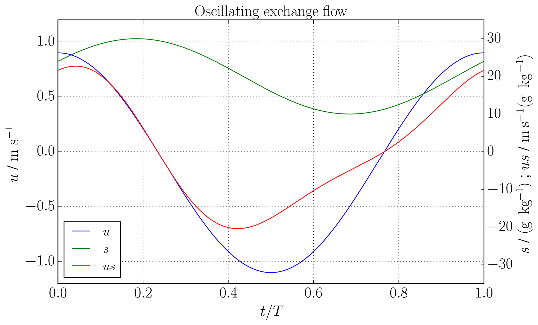
Figure 1 shows an example for u(t), s(t) and u(t)⋅s(t), with A=10 000 m2, m s−1, ua=1 m s−1, sr=20 g kg−1 and sa=10 g kg−1, resulting in . In this case, Q(S), Qs(S) and Sdiv can be calculated analytically by either (5) or (7) (see Appendix A) and are shown in Fig. 2d. By means of (4), the inflow and outflow volume fluxes and salinities, Qin, Qout, sin and sout, can then be exactly calculated. The resulting analytical TEF bulk values are Qin=813.240 m3s−1, m3s−1, sin=28.424 g kg−1 and sout=12.748 g kg−1.
We created a time series of I=105 time steps of (8) and computed q(S) and qs(S) for a varying number N of salinity classes between Smin=10 g kg−1 and Smax=31 g kg−1; see Fig. 2. In Fig. 2a (N=128), the small N leads to smooth profiles for both q and Q. Profiles of higher numbers (N=1024, N=8192) of salinity classes exhibit more noisy q but apparently still smooth Q (Fig. 2b, c). Comparison with the analytical solution (Fig. 2d) shows that Q is similar for all N and q becomes more noisy. This is a result of the numerical discretisation of the data. Most likely, the numerical values (e.g. due to round-off errors) for these salinities are all different. Other than in continuous salinity space where inflows and outflows in the same salinity class partially compensate for one another, the corresponding discrete values could be associated with different salinity classes and the compensation does not occur anymore, resulting in noisy profiles, which leads to errors in the results of the sign method. Q only appears to be smooth, but the noise is of course apparent since Q and q are dependent on each other. The integration process of the discrete qc (see (3)) smooths the resulting Qc.
To study the convergence of the two different methods (the sign method and dividing salinity method), one can compare the errors in discrete form to the analytical values. Figure 3 shows the relative error, , of the numerically computed inflow bulk values depending on the number of time steps I and the number of salinity classes N. For this analytical scenario, both methods coincide for a small number of salinity classes. For increasing N, the error of the sign method increases beyond a critical number of salinity classes and converges to the error of the absolute values (black line, 6), whereas the dividing salinity method converges towards a small constant relative error. The critical point where the error of the sign method increases is different for each number of time steps. The convergence analysis for different numbers of time steps I is done to gain experience in the impact of temporal resolution of the oscillating flow on the final bulk values. With the time step here being the equivalent to the output interval of a hydrodynamic model which provides data for TEF, the findings can directly be transferred to the analysis of model data. The error of the dividing salinity method decreases continuously with an increasing number of time steps I, showing that indeed the dividing salinity method converges towards the correct bulk values. Interestingly, there is almost no difference for I=103 and I=104, and I=105 and I=106, for the dividing salinity method, which is due to the compensation of the added values in the data of u(t) and s(t). For this scenario of a well-mixed estuary, one tidal period should be resolved with at least 1000 time steps, meaning one data point every minute or less, to find the transport Qin with an error less than 0.1 % with the dividing salinity method. This is due the strong time dependency on the problem. For a stationary problem, one point in time would be sufficient to find the correct exchange flow.

Figure 2Oscillating exchange flow (see Sect. 2): from (14) and (15) numerically (a–c) and analytically (d) found Q(S) (blue), q(S) (green), dividing salinity, Sdiv (dashed, red), for I=104 time steps for one tidal cycle and varying number of salinity classes N. With increasing N, q becomes more noisy, whereas Q seems unchanged.
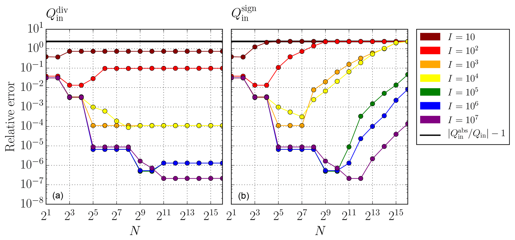
Figure 3Oscillating exchange flow (see Sect. 2): relative error of Qin computed with (a) the dividing salinity method and (b) the sign method depending on the number of time steps I (colour) and salinity classes N. The sign method (5) and the dividing salinity method (7) coincide for a small number of salinity classes, but the error of the sign method converges in the limit of large N towards the error of the absolute bulk values (black line, 6). In contrast, the error of the dividing salinity method converges towards a constant value. The errors of both methods decrease with increasing number of time steps I.
3.1 Mathematical formulation
Encouraged by the good convergence behaviour of the dividing salinity method demonstrated in the previous section, we introduce here a general formulation which includes inverse estuaries and exchange flows with more than two layers. The general idea is to identify the salinities which divide qc into inflowing and outflowing parts. This corresponds to zero crossings, dividing qc>0 and qc<0. Analytically, the zero crossings are calculated by solving qc(Sdiv)=0 for Sdiv. However, as the discrete qc might be very noisy with too many zero crossings (see Sect. 2), we propose finding the extrema of the discrete Qc profiles, which share the same salinities as the zero crossings. Figure 4 shows a hypothetical exchange flows of four layers, separated by five dividing salinities which can be sorted in ascending order: . The fluxes in each layer can be calculated by
In the next step, inflow segments with and outflow segments with can be identified and indexed. For the example in Fig. 4, we index starting from Smin: , , and . The representative salinities are calculated for each inflow and outflow similar to (4):
where m denotes the index with and so on. For a classical estuary, (11) reads as (7), where the only dividing salinity except Smin or Smax is .
The mixing relations of MacCready et al. (2018) and Burchard et al. (2019) require only one value each for the inflow properties and outflow properties, respectively. These can be obtained from a multi-layer transect by applying weighted averages, i.e. for the inflowing bulk values:
and accordingly for and cout.
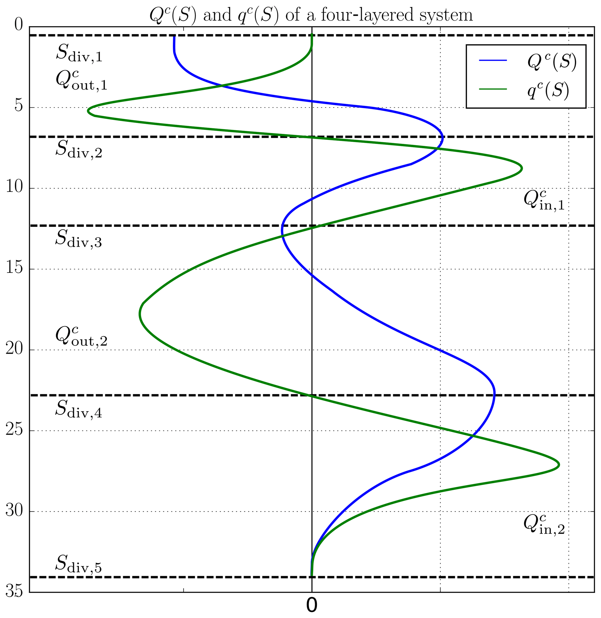
Figure 4Sketch of hypothetical TEF profiles of a four-layered system with alternating inflows and outflows, and . The respective inflows and outflows are divided by the zero crossings of qc(S) (green), so-called dividing salinities, Sdiv, j (dashed, black), which correspond to the minima and maxima of Qc(S) (blue).
3.2 Discrete formulation
The output from a numerical model along a transect across an estuary is assumed to consist of I time steps with and , which are spatial increments per each time step. The output should include collocated model data (salinity), (tracer) and (incoming normal velocity) which are available on cross-sectional area increments . The salinity interval , with and , where and , is divided into N equidistant intervals of length ; compare Fig. 5. The discrete profiles of qc should be obtained directly without numerically calculating the volume flux profile Qc before to avoid truncation errors due to numerical derivatives and to save computational time:
where ⌊⋅⌋ is the integer truncation function. With this, the tracer flux increments are directly added to the respective salinity class; see the dots in the sketch of Fig. 5. Computation of Qc(S) can be easily carried out by summation of :
Using the extended dividing salinity method defined in (11), the calculation for the transport reads
where ndiv, j and describe the indexes, where two consecutive extrema of Qc are located. The dividing salinity indices are calculated with an algorithm which searches Q for local extrema by comparing every entry to its nearest neighbours ( and ). If is greater (smaller) than its two neighbours, is stored as ndiv, j and denoted maximum (minimum). Afterwards, transport is computed according to (16), and only dividing salinities with transport greater than a threshold transport Qthresh are considered. Please see Appendix B for a detailed description.
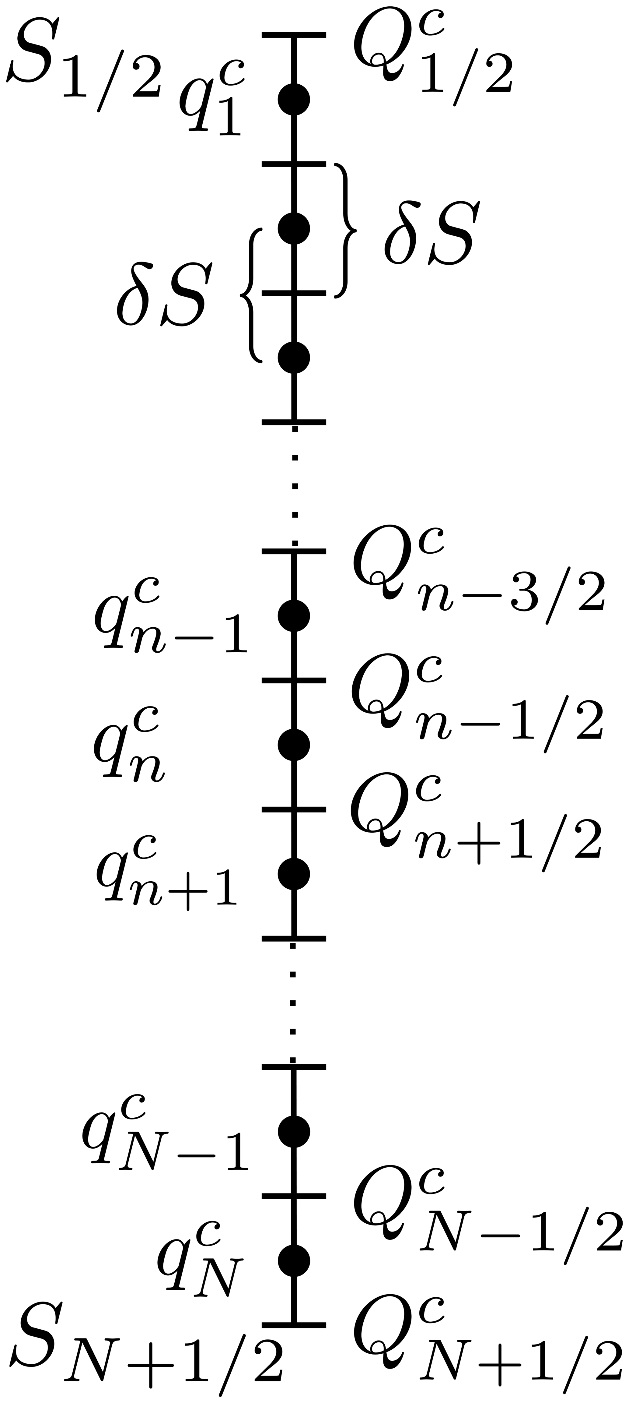
Figure 5Sketch of how Qc and qc are located in a discrete salinity space. The salinity interval [] is divided into N equidistant salinity classes of length δS. The entries of Qc () are located on the lines, and the entries of qc () are located on the dots.
The Baltic Sea, shown in Fig. 6, can be considered as a large estuary with a long-term averaged river runoff of around 16 000 m3s−1 and about balanced precipitation and evaporation (Matthäus and Schinke, 1999). In the estuarine classification diagram by Geyer and MacCready (2014), the Baltic Sea has been classified as a fjord type and a strongly stratified estuary, due to its relatively low runoff and relatively low mixing. The topography of the Baltic Sea consists of several basins of which the Gotland Basin in the central Baltic Sea, denoted as GB in Fig. 6, is the largest with a water depth of about 240 m. The shallow and narrow Danish Straits in the southwest provide the only connection to the saline North Sea.
Episodic inflow events of water consisting of a mixture of saline North Sea water and recirculated brackish Baltic Sea water (Meier et al., 2006) transport large amounts of salt and oxygen into the Baltic Sea. These inflows may either occur as major Baltic inflows (MBIs; i.e. as well-mixed, barotropic inflows) during winter months (Matthäus and Schinke, 1999; Mohrholz et al., 2015) or as baroclinic summer inflows (Feistel et al., 2004, 2006). These large inflow events propagate as dense bottom currents from basin to basin, where they are subject to entrainment of overlaying less saline water. The volume of the inflows increases and their salinity decreases on the way into the central Baltic Sea, where they ventilate the typically anoxic bottom layers (Reissmann et al., 2009). More frequent but weaker and less saline inflow events propagate through the western Baltic Sea (Sellschopp et al., 2006; Umlauf et al., 2007) and have the potential to ventilate intermediate layers but not the bottom layers in the central Baltic Sea (Reissmann et al., 2009). The major mixing process to transport saline bottom waters towards the surface of the central Baltic Sea has been identified as boundary mixing (Holtermann et al., 2012, 2014). However, recently double diffusion in the stratified interior has been discussed as another possibly efficient mixing process in the Baltic Sea (Umlauf et al., 2018). Finally, various surface mixed layer processes mix the salt into the surface layer of the Baltic Sea, such that a horizontal surface salinity gradient is established, with salinities varying from 25 g kg−1 in the Kattegat (K) to 5 g kg−1 in the Bothnian Bay (BoB). A permanent halocline separates these surface waters from the saline bottom waters. The halocline is located approximately in 70–90 m depth in the Gotland Basin. In addition, a seasonal thermocline develops during summer between 10 and 30 m (Reissmann et al., 2009). At times, salinity inversions occur in the strongly stratified thermocline, with surface waters being slightly more saline than waters in the thermocline (Burchard et al., 2017).
Above the halocline, driven by wind, inflows and Earth rotation, a cyclonic circulation is generally present in the central Baltic Sea, with net northward flow in the east of Gotland and southward flow in the west of Gotland (Meier, 2007; Omstedt et al., 2014). This cyclonic circulation is also present in the deeper layers of the central Baltic Sea, possibly driven by inflows and boundary mixing processes (Hagen and Feistel, 2007; Meier, 2007; Holtermann and Umlauf, 2012). This deep-water mean circulation is overlaid by topographic waves and inertial oscillations (Holtermann et al., 2014).
In the following, the numerical properties of the TEF analysis framework are tested against two transects of the Baltic Sea. The first transect is located across Darss Sill (D, red transect) in the western Baltic Sea over which part of the exchange with the North Sea is occurring; see Sect. 4.1. The second transect (green) is located in the Gotland Basin where we apply the extended dividing salinity method to the complicated multi-layer current system; see Sect. 4.2.
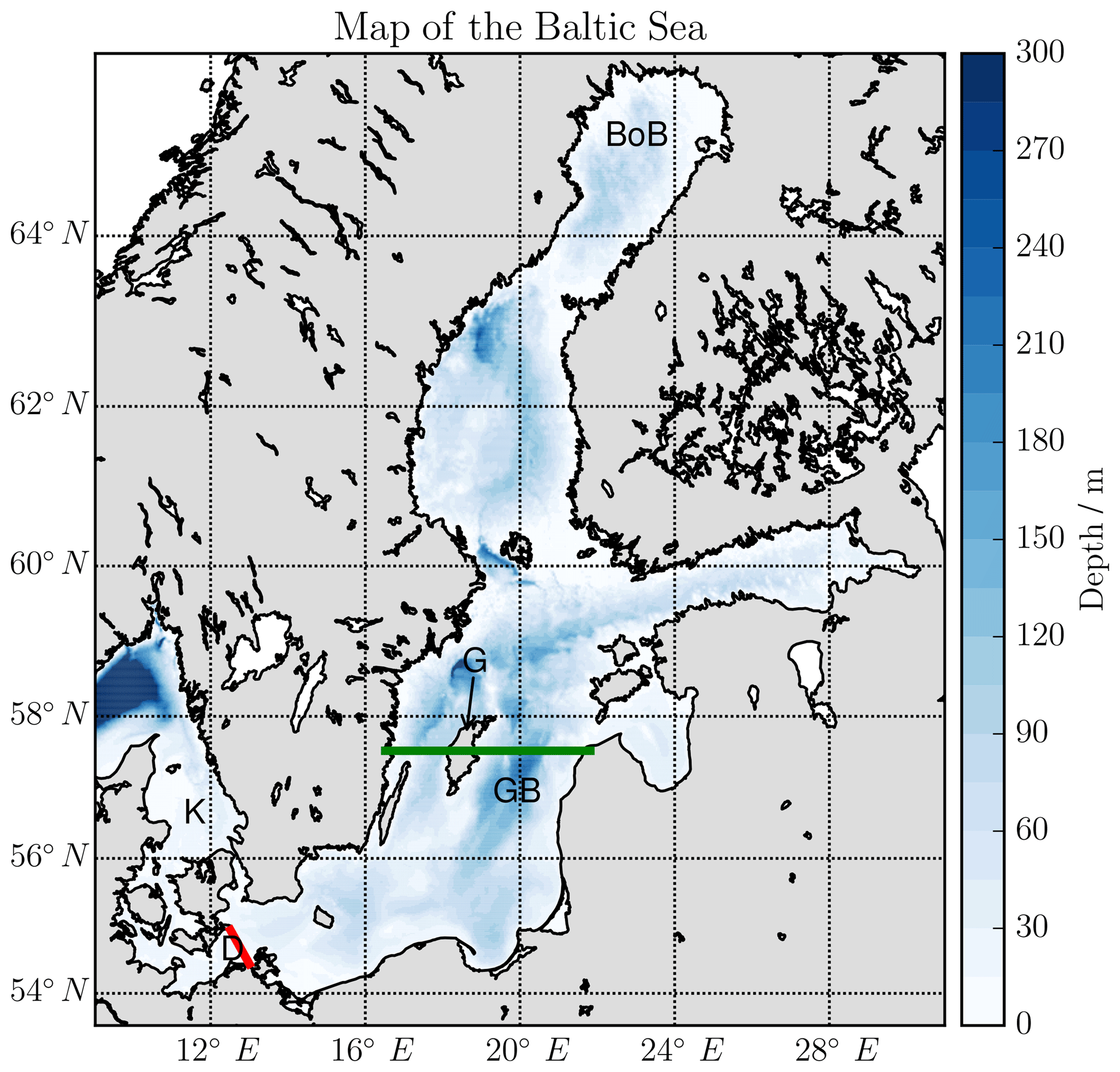
Figure 6Map and bathymetry of the Baltic Sea. K: Kattegat, D: Darss Sill and the Darss Sill transect (red), G: the Gotland island, GB: Gotland Basin and the Gotland transect (green), BoB: Bothnian Bay.
4.1 Exchange flow over Darss Sill
In their recent review paper, Burchard et al. (2018) applied the Knudsen relations and the TEF analysis framework to analyse 65 years of high-resolution numerical model output for the western Baltic Sea using the General Estuarine Transport Model (GETM) (Burchard and Bolding, 2002; Hofmeister et al., 2010; Klingbeil and Burchard, 2013). Here, we investigate numerical properties of the TEF calculations based on the same numerical model output for the complex inflow years (2002/2003) with several barotropic and baroclinic inflows (Feistel et al., 2006) over the Darss Sill transect shown in Fig. 6.
The horizontal resolution of the model is about 600 m, and the water column is discretised by 42 vertical adaptive layers, the thickness of which vary in time and space (Gräwe et al., 2015). The salinity, velocity and layer thickness data are interpolated to 95 locations equally spaced by Δx=545 m along the 52 km long Darss Sill transect which is directed in northwest–southeast direction, such that the number of data points per time step is . The model output time step is Δt=3 h, such that I=5840 time steps for two simulation years are stored. These 3-hourly values are obtained by thickness-weighted averaging (Klingbeil et al., 2019) of the model layer values from all model time steps within the output interval.
Application of the TEF analysis framework for N different salinity classes is shown in Fig. 7, where a classical two-layer exchange flow with inflow at high salinities is seen. The upper panels show q and the respective TEF bulk values, computed with the sign method. q becomes more noisy with increasing N. The bulk values still change with increasing N. The lower panels show Q for the same N and the TEF bulk values computed with the extended dividing salinity method. These bulk values do converge for increasing N towards constant values. For this case, Qthresh was set to Qthresh=100 m3 s−1.
The values found in this study with the dividing salinity method confirm that the found bulk values in Burchard et al. (2018) are correct and did not experience great errors from using the sign method.
Similar to the dependency of the TEF bulk values on I in the oscillating exchange flow in Sect. 2, we investigate the dependency of the TEF bulk values on the temporal resolution of the exchange flow. In order to do so, we repeated the TEF analyses for data obtained by thickness-weighted averaging of the 3-hourly model output to intervals of 12 h, and 1, 3, 5 and 10 d. For the dividing salinity method, the relative differences to estimated reference values for different time steps of the model output are calculated. The reference bulk values have been calculated by the dividing salinity method for salinity classes and the 3-hourly output, since the exact values are not available. The hydrodynamic model was forced with 3-hourly atmospheric data, meaning that external processes of smaller timescales are not included. Therefore, the estimated bulk values can be considered as good estimations. Figure 8a shows Q(S, Δt) with the corresponding dividing salinities. With coarser temporal resolution (larger Δt), the maximum of Q moves towards greater salinities and smaller transport values, showing a weakened exchange flow. For Δt=10 d, the maximum shifts back to smaller salinities, indicating that some processes are not resolved anymore. Furthermore, the maximum salinities decrease with reduced temporal resolution, which indicates that the inflows of high salinities are not captured. In Fig. 8b, the relative deviations of the TEF bulk values are shown for the inflow. With increasing time step Δt, the deviations increase rapidly as one would expect since processes of smaller timescales are not resolved anymore. For Δt≥3 d, the deviations fluctuate around a constant value with the exception of Δt=5 d. The deviations for this time step are smaller than expected. Figure 8a shows that the shape of Q(S, 5 d) is closer to the shape of the 3-hourly output, leading to more correct bulk values, which we expect to be accidental. The properties of the outflow follow a similar pattern with generally smaller deviations since the outflow does not depend as much on inflows events (not shown here). Figure 8b also shows that for this simulation 12-hourly model output is enough to resolve the exchange flow properly, i.e. errors of less than 1 %.
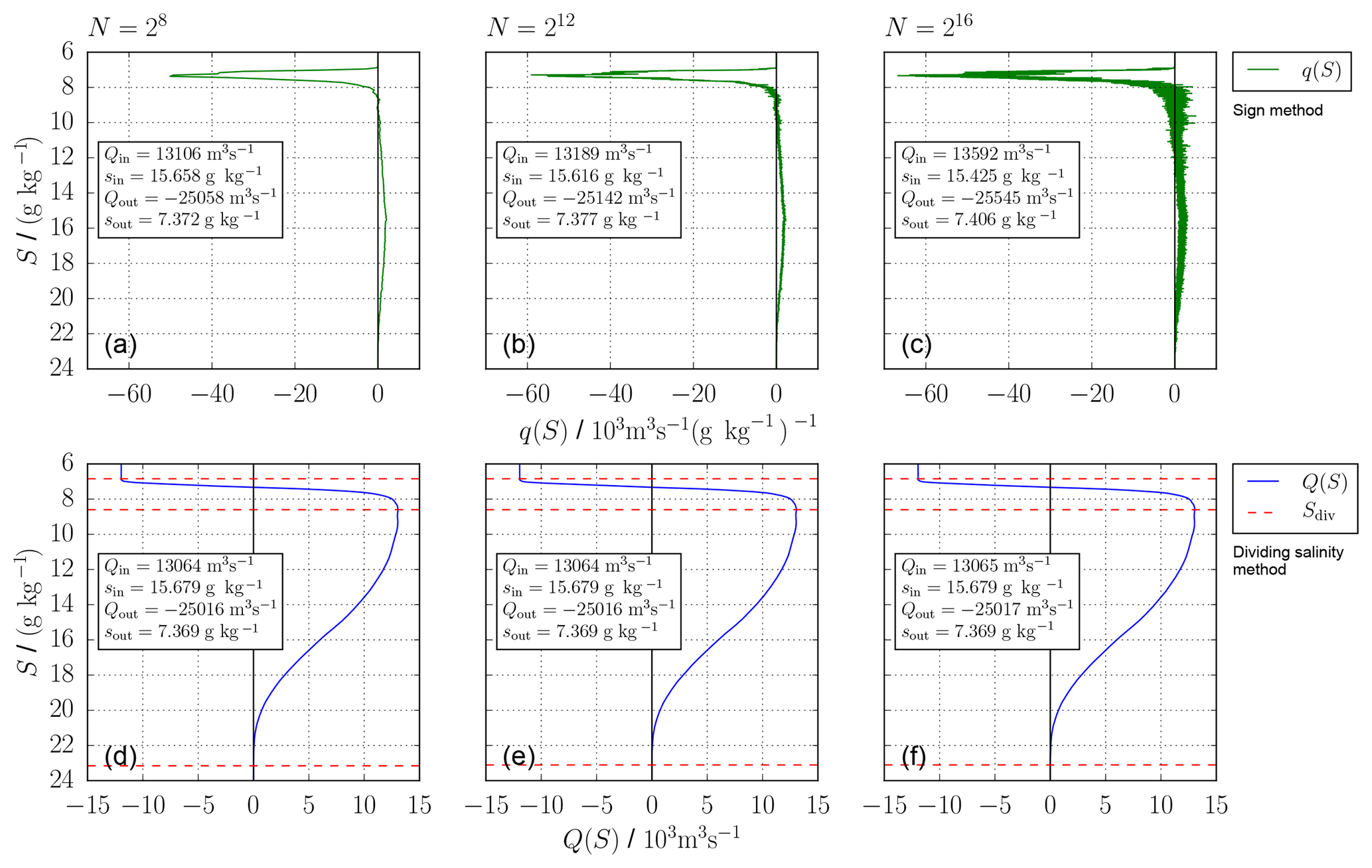
Figure 7Exchange flow over Darss Sill: profiles of q (a, b, c) and Q (d, e, f) for the Darss Sill transect in 2002/2003 depending on the number of salinity classes N: (a, d) , (b, e) , (c, f) . The respective TEF bulk values are calculated with the sign method (5) in panels (a, b, c) and the extended dividing salinity method (11, 16) in panels (d, e, f).
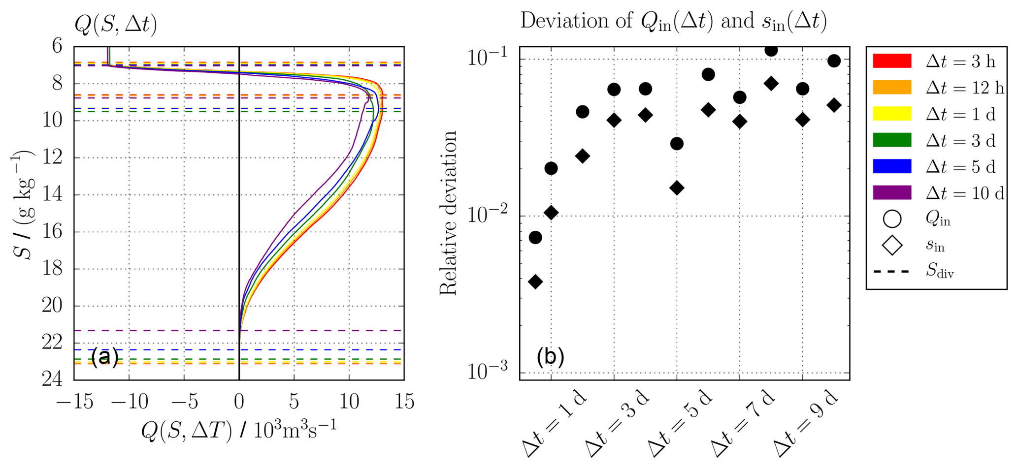
Figure 8Exchange flow over Darss Sill: comparison of Q(S) () for different Δt in panel (a) and the relative deviations of Qin and sin in dependency Δt to the bulk values for Δt=3 h in panel (b). The bulk values were computed from Q(Δt) using the extended dividing salinity method (11, 16). The dashed lines in panel (a) show the dividing salinities used to compute the bulk values in panel (b). With different temporal resolutions, the shape of Q(S) changes considerably and the resulting bulk values deviate significantly from the ones for 3-hourly data.
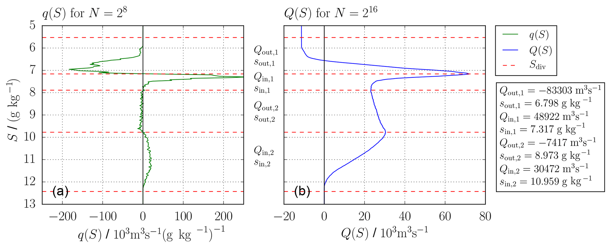
Figure 9Cross section through Gotland Basin: profiles of q for (a) and Q for (b) for the Gotland transect in 2002/2003. Five dividing salinities separate two inflows and two outflows. The corresponding TEF bulk values are listed on the right.
4.2 Cross section through the Gotland Basin
In this section, the capability of the extended dividing salinity method to be applied to exchange flows or transects with more than two layers is demonstrated. Here, example results are shown for model data of the Gotland Basin in the Baltic Sea. The analysed transect uses the model run from Burchard et al. (2018) consisting of 156 equally spaced locations with 1 nmi resolution and 50 vertical adaptive layers. Daily averages from 2 simulation years, 2002 and 2003, are analysed. These 2 years show a complex inflow activity, with baroclinic inflows during summer 2002 and summer 2003 and an MBI during winter 2002/2003 (Feistel et al., 2006).
Figure 9a shows q for salinity classes to visualise the exchange flow, whereas Fig. 9b shows Q for , which is used to compute the bulk values using the extended dividing salinity method (11 and 16). For this data set, five dividing salinities are found using m3 s−1, separating two inflows (Qin, 1 and Qin, 2) and two outflows (Qout, 1 and Qout, 2). These are listed with their respective salinities (sin, 1, sin, 2, sout, 1 and sout, 2) on the right of Fig. 9 for N=216 salinity classes.
The net southward transport of 11 300 m3 s−1 results from the fact that most river input is entering the Baltic Sea north of the transect. Qin, 1 and Qout, 1 belong to the cyclonic surface circulation of the Gotland Basin described above. With the main river input in the north, the outflow Qout, 1 is less saline than the inflow Qin, 1 which experiences more entrainment of saline bottom waters during the recirculation. Qin, 2 describes the net northward transport of the deep circulation which is fed with high salinities of the inflow events. Qout, 2 is the corresponding deep net southward transport of less saline water which is homogeneous over a salinity range from ∼8 to ∼10 g kg−1; see Fig. 9a. Further and more detailed TEF analyses of the dynamics in the Gotland Basin should be carried out in the future but will be not part of this study, as the focus lies on the method and not the physics. Nevertheless, the extended dividing salinity method proves to be suitable to find robust bulk values for multi-layered exchange flows.
This study investigated the numerical issues of the TEF analysis framework, proposed by MacCready (2011). Two existing calculation methods for the computation of the bulk values of an exchange flow, the sign method (5) (MacCready, 2011) and the dividing salinity method (7) (MacCready et al., 2018), were compared in their respective convergence behaviours for an analytical test case. We could show that only the dividing salinity method converges towards the analytical bulk values. The sign method relies on a smooth q profile, but q tends to become more noisy with increasing number of salinity classes (for constant temporal resolution), which leads to wrong convergence. The dividing salinity method on the other hand relies on a smooth Q. Although q is very noisy for a high number of salinity classes, Q allows a convergent and robust calculation of TEF bulk values. An extended formulation of the dividing salinity method is presented which includes exchange flows of more than two layers as well as inverse exchange flows. We showed the application to two transects of the Baltic Sea. The main challenge of the extended dividing salinity method is finding the dividing salinities. We provide a detailed description of a robust algorithm to obtain extrema of Q which is required to determine the dividing salinities in Appendix B. Moreover, we investigated the dependency of the calculated bulk values on the frequency of model output. The results confirm that the output of the model for a transect which should be analysed by the application of TEF is strongly dependent on the physical mechanism controlling the exchange flow.
Based on our results, we propose a best-practice procedure for calculating TEF from a numerical model:
-
At the level of setting up a numerical model, the spatial (horizontal and vertical) resolution should be chosen as high as possible to reproduce return flows due to lateral eddies and smaller overturns.
-
Once a transect for the TEF analysis has been identified, the frequency for storing the output along that transect has to be chosen. For analytical correctness, the binning of data of volume and salt fluxes into salinity classes should be done online within the hydrodynamic model at every model time step. Time-averaged model output of these binned data can directly be used for the TEF analysis. If the model only provides output within the model layers, the binning and averaging must be done offline during postprocessing. This would induce different kinds of errors: (i) instantaneous data snapshots which skip intermediate model time steps do not conserve fluxes and do not consider intermediate salinity variations; (ii) model data obtained by thickness-weighted averaging over model time steps conserve fluxes but merge data of different salinities. Both types of errors can be reduced with a sufficiently high output frequency, such that the output data still resolve the dynamics of the flow.
-
If the binning is not done online, required output fields are the velocity component normal to the transect, the salinity and the grid box area along the transect. We suggest that these variables are stored as thickness-weighted averaged values (Klingbeil et al., 2019) between two output time steps to ensure the conservation of volume and salinity.
-
The results should be analysed for a large range of salinity classes N with the dividing salinity method (11) and (12) to check the convergence of the TEF bulk values. In this study, N≈1000 salinity classes ( g kg−1) were sufficient enough for all three investigated examples with errors or deviations smaller than 0.1 %.
-
Visualisation of the exchange flow should still be done with a smooth q, since it shows the inflows and outflows more clearly. We suggest to choose N≈250 for estuaries with a wide range of salinities or a step size in salinity space of ∼0.05 g kg−1, i.e. 20 steps per 1 g kg−1, for estuaries with smaller salinity ranges.
Please request the authors if you are interested in the code used for this publication.
For the oscillating exchange flow given in (8), the analytical solution is given here for the volume flux profile Q(S) and the salinity flux profile Qs(S). According to (1), these profiles are calculated as
and
with
which ensures that s(t)≥S for and s(t)<S for . q(S) is calculated according to (2):
The dividing salinity can be calculated by finding the root of q(S). Solving (A4) with q(Sdiv)=0 for Sdiv:
The TEF bulk values can be calculated according to (7) and (4).
The algorithm finding the extrema of Q works as follows. First, every entry of Q is compared with its nearest neighbours and . If is either the maximum (minimum) in this interval, the index is stored and denoted by max (min), respectively. Afterwards, consecutive maxima or minima are deleted, leaving only the greatest maxima or the smallest minima. Now, minima and maxima should be alternating. At this stage, there are probably physically insignificant extrema found. Therefore, transport is calculated according to (16); their absolute values |ΔQj| are compared to a given threshold value Qthresh, which we recommend to set to a value of m3 s−1. If the transport |ΔQj| is smaller than Qthresh, Q(Sdiv, j) and are compared and only the greater (smaller) of the two is kept to ensure that the greater maxima (smaller minima) remains. The two dividing salinities which belong to the smaller (greater) transport are then not considered anymore. If the first or last extremum is involved in this procedure, only the extremum which is not the first or last extremum is deleted. If this needs to be done, then the first or last extremum changes its property from either minimum to maximum or the other way round to ensure alternating minima and maxima. The last step is to adjust the first and last extrema to the index where starts to differ from Q1∕2 (low salinities) or where differs from 0 (high salinities). This step is not necessary for calculating the correct TEF bulk values since only the dividing part is important and not the exact value of the dividing salinity. Nevertheless, this procedure ensures that Sdiv, 1 is the salinity class next to min(s) and is next to max(s), with J being the number of layers.
Figure B1 shows the sensitivity of the number of dividing salinities on Qthresh for the data from Sect. 4.1 for N=4096 salinity classes. In Fig. B1a, for m3 s−1 (to filter out numerical noise of double-precision data), 135 dividing salinities, most between 8 and 10 g kg−1, are found. Most of them are noise carried on from the q profile to Q and have no physical meaning. However, two major transport values are found: −24 885 and 12 603 m3 s−1. For Qthresh=25 m3 s−1, noise-related transport values are filtered out, leaving two small transport values of 63 and −44 m3 s−1. The two main transport values change to −25 016 and 13 045 m3 s−1. Increasing to Qthresh=50 m3 s−1, the −44 m3 s−1 is not accounted for, and according to the algorithm the two involved dividing salinities are deleted. This deletes the 63 m3 s−1 transport as well. As a result the net transport of 19 m3 s−1, transport is now accounted to the major inflow, which increased from 13 045 to 13 064 m3 s−1 if compared to Fig. B1b. These are the exact same results as Fig. 7b, where Qthresh=100 m3 s−1 was used.
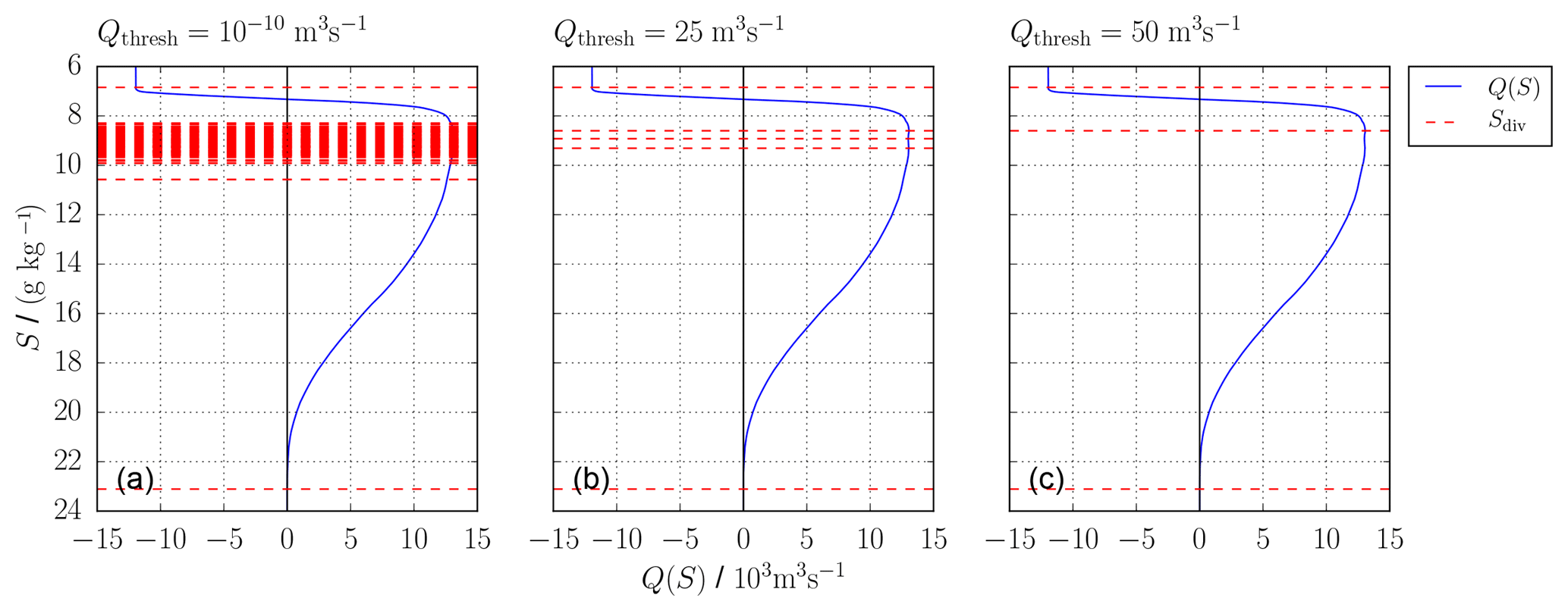
Figure B1Comparison of the algorithm for (a) m3 s−1, (b) Qthresh=25 m3 s−1 and (c) Qthresh=50 m3 s−1 for the Darss Sill data with N=4096. The number of dividing salinities decreases with increasing threshold transport.
The authors declare that they have no conflict of interest.
This paper is a contribution to BMBF-GROCE FKZ 03F0778. Hans Burchard and Marvin Lorenz were supported by Research Training Group Baltic TRANSCOAST GRK 2000 funded by the German Research Foundation. Knut Klingbeil was supported by the Collaborative Research Centre TRR 181 on Energy Transfer in Atmosphere and Ocean funded by the German Research Foundation (project no. 274762653), and Parker MacCready was supported by US National Science Foundation (grant no. OCE-1736242).
The publication of this article was funded by the Open Access Fund of the Leibniz Association.
This paper was edited by Eric J. M. Delhez and reviewed by two anonymous referees.
Burchard, H. and Bolding, K.: GETM, A General Estuarine Transport Model: Scientific Documentation, Tech. Rep. EUR 20253 EN, Eur. Comm., 2002. a
Burchard, H., Basdurak, N. B., Gräwe, U., Knoll, M., Mohrholz, V., and Müller, S.: Salinity inversions in the thermocline under upwelling favorable winds, Geophys. Res. Lett., 44, 1422–1428, 2017. a
Burchard, H., Bolding, K., Feistel, R., Gräwe, U., Klingbeil, K., MacCready, P., Mohrholz, V., Umlauf, L., and van der Lee, E. M.: The Knudsen theorem and the Total Exchange Flow analysis framework applied to the Baltic Sea, Prog. Oceanogr., 165, 268–286, https://doi.org/10.1016/j.pocean.2018.04.004, 2018. a, b, c, d
Burchard, H., Lange, X., Klingbeil, K., and MacCready, P.: Mixing Estimates for Estuaries, J. Phys. Oceanogr., 49, 631–648, https://doi.org/10.1175/JPO-D-18-0147.1, 2019. a, b
Döös, K. and Webb, D. J.: The Deacon cell and the other meridional cells of the Southern Ocean, J. Phys. Oceanogr., 24, 429–442, 1994. a
Feistel, R., Nausch, G., Heene, T., Piechura, J., and Hagen, E.: Evidence for a warm water inflow into the Baltic Proper in summer 2003, Oceanologia, 46, 581–598, 2004. a
Feistel, R., Nausch, G., and Hagen, E.: Unusual Baltic inflow activity in 2002-2003 and varying deep-water properties, Oceanologia, 48, 21–35, 2006. a, b, c
Geyer, W. R. and MacCready, P.: The estuarine circulation, Annu. Rev. Fluid Mech., 46, 175–197, 2014. a
Gräwe, U., Holtermann, P., Klingbeil, K., and Burchard, H.: Advantages of vertically adaptive coordinates in numerical models of stratified shelf seas, Ocean Model., 92, 56–68, 2015. a
Hagen, E. and Feistel, R.: Synoptic changes in the deep rim current during stagnant hydrographic conditions in the Eastern Gotland Basin, Baltic Sea, Oceanologia, 49, 185–208, 2007. a
Hofmeister, R., Burchard, H., and Beckers, J.-M.: Non-uniform adaptive vertical grids for 3-D numerical ocean models, Ocean Model., 33, 70–86, 2010. a
Holtermann, P. L. and Umlauf, L.: The Baltic Sea Tracer Release Experiment: 2. Mixing processes, J. Geophys. Res.-Oceans, 117, https://doi.org/10.1029/2011JC007445, 2012. a
Holtermann, P. L., Umlauf, L., Tanhua, T., Schmale, O., Rehder, G., and Waniek, J. J.: The Baltic Sea Tracer Release Experiment: 1. Mixing rates, J. Geophys. Res.-Oceans, 117, https://doi.org/10.1029/2011JC007439, 2012. a
Holtermann, P. L., Burchard, H., Graewe, U., Klingbeil, K., and Umlauf, L.: Deep-water dynamics and boundary mixing in a nontidal stratified basin: A modeling study of the Baltic Sea, J. Geophys. Res.-Oceans, 119, 1465–1487, 2014. a, b
Klingbeil, K. and Burchard, H.: Implementation of a direct nonhydrostatic pressure gradient discretisation into a layered ocean model, Ocean Model., 65, 64–77, 2013. a
Klingbeil, K., Becherer, J., Schulz, E., de Swart, H. E., Schuttelaars, H. M., Valle-Levinson, A., and Burchard, H.: Thickness-Weighted Averaging in tidal estuaries and the vertical distribution of the Eulerian residual transport, J. Phys. Oceanogr., accepted, 2019. a, b, c, d
Knudsen, M.: Ein hydrographischer Lehrsatz, Annalen der Hydrographie und Maritimen Meteorologie, 28, 316–320, 1900. a, b, c
Knuth, K. H.: Optimal Data-Based Binning for Histograms, arXiv e-prints, physics/0605197, 2006. a
MacCready, P.: Calculating estuarine exchange flow using isohaline coordinates, J. Phys. Oceanogr., 41, 1116–1124, 2011. a, b, c, d, e
MacCready, P., Rockwell Geyer, W., and Burchard, H.: Estuarine Exchange Flow is Related to Mixing through the Salinity Variance Budget, J. Phys. Oceanogr., 48, 1375–1384, 2018. a, b, c, d, e, f
Matthäus, W. and Schinke, H.: The influence of river runoff on deep water conditions of the Baltic Sea, in: Biological, Physical and Geochemical Features of Enclosed and Semi-enclosed Marine Systems, edited by Blomqvist, E. M., Bonsdorff, E., and Essink, K., 1–10, Springer Netherlands, Dordrecht, 1999. a, b
Meier, H. E. M.: Modeling the pathways and ages of inflowing salt-and freshwater in the Baltic Sea, Estuarine Coast. Shelf Sci., 74, 610–627, 2007. a, b
Meier, H. M., Feistel, R., Piechura, J., Arneborg, L., Burchard, H., Fiekas, V., Golenko, N., Kuzmina, N., Mohrholz, V., Nohr, C., Paka, T. V., Sellschopp, J., Stips, A., and Zhurbas, V.: Ventilation of the Baltic Sea deep water: A brief review of present knowledge from observations and models, Oceanologia, 48, 2006. a
Mohrholz, V., Naumann, M., Nausch, G., Krüger, S., and Gräwe, U.: Fresh oxygen for the Baltic Sea – an exceptional saline inflow after a decade of stagnation, J. Marine Syst., 148, 152–166, 2015. a
Omstedt, A., Elken, J., Lehmann, A., Leppäranta, M., Meier, H., Myrberg, K., and Rutgersson, A.: Progress in physical oceanography of the Baltic Sea during the 2003–2014 period, Prog. Oceanogr., 128, 139–171, 2014. a
Purkiani, K., Becherer, J., Flöser, G., Gräwe, U., Mohrholz, V., Schuttelaars, H. M., and Burchard, H.: Numerical analysis of stratification and destratification processes in a tidally energetic inlet with an ebb tidal delta, J. Geophys. Res.-Oceans, 120, 225–243, 2015. a
Reissmann, J. H., Burchard, H., Feistel, R., Hagen, E., Lass, H. U., Mohrholz, V., Nausch, G., Umlauf, L., and Wieczorek, G.: Vertical mixing in the Baltic Sea and consequences for eutrophication – A review, Prog. Oceanogr., 82, 47–80, 2009. a, b, c
Sellschopp, J., Arneborg, L., Knoll, M., Fiekas, V., Gerdes, F., Burchard, H., Lass, H. U., Mohrholz, V., and Umlauf, L.: Direct observations of a medium-intensity inflow into the Baltic Sea, Cont. Shelf Res., 26, 2393–2414, 2006. a
Umlauf, L., Arneborg, L., Burchard, H., Fiekas, V., Lass, H., Mohrholz, V., and Prandke, H.: Transverse structure of turbulence in a rotating gravity current, Geophys. Res. Lett., 34, https://doi.org/10.1029/2007GL029521, 2007. a
Umlauf, L., Holtermann, P. L., Gillner, C. A., Prien, R., Merckelbach, L., and Carpenter, J. R.: Diffusive convection under rapidly varying conditions, J. Phys. Oceanogr., 48, 1731–1747, 2018. a
Walin, G.: A theoretical framework for the description of estuaries, Tellus, 29, 128–136, 1977. a, b, c
Walin, G.: On the deep water flow into the Baltic, Geofysica, 17, 75–93, 1981. a
- Abstract
- Introduction
- Convergence analysis for an analytical classical exchange flow
- Extended dividing salinity method
- Application to exchange flow in the Baltic Sea
- Discussion and conclusions
- Code availability
- Appendix A: Analytical solution for Q(S) and Qs(S)
- Appendix B: Algorithm description
- Competing interests
- Acknowledgements
- Financial support
- Review statement
- References