Estimation of geostrophic current in the Red Sea based on sea level anomalies derived from extended satellite altimetry data

Geostrophic current data near the coast of the Red Sea have large gaps. Hence, the sea level anomaly (SLA) data from Jason-2 have been reprocessed and extended towards the coast of the Red Sea and merged with AVISO data at the offshore region. This processing has been applied to build a gridded dataset to achieve the best results for the SLA and geostrophic current. The results obtained from the new extended data at the coast are more consistent with the observed data (conductivity–temperature–depth, CTD) and hence geostrophic current calculation. The patterns of SLA distribution and geostrophic currents are divided into two seasons: winter (October–May) and summer (June–September). The geostrophic currents in summer are flowing southward over the Red Sea except for narrow northward flow along the east coast. In winter, currents flow to the north for the entire Red Sea except for a small southward flow near the central eastern and western coast. This flow is modified by the presence of cyclonic and anticyclonic eddies, which are more concentrated in the central and northern Red Sea. The results show anticyclonic eddies (AEs) on the eastern side of the Red Sea and cyclonic eddies (CEs) on the western side during winter. In summer, cyclonic eddies are more dominant for the entire Red Sea. The result shows a change in some eddies from anticyclonic during winter to cyclonic during summer in the north between 26.3 and 27.5^∘ N. Furthermore, the life span of cyclonic eddies is longer than that of anticyclonic eddies.

1 Introduction

The Red Sea is a narrow semi-enclosed water body that lies between the continents of Asia and Africa. It is located between 12.5–30^∘ N and 32–44^∘ E in a NW–SE orientation. Its average width is 220 km and the average depth is 524 m (Patzert, 1974). It is connected at its northern end with the Mediterranean Sea through the Suez Canal and at its southern end with the Indian Ocean through the strait of Bāb al Mandab. The exchange of water through Bāb al Mandab (shallow sill of 137 m) is the most significant factor that determines the oceanographic properties of the Red Sea (Smeed, 2004).

During winter, the southern part of the Red Sea is subject to SE monsoon wind, which is relatively strong from October to December, with a speed of 6.7–9.3 m s⁻¹ (Patzert, 1974). During the summer season, the wind shifts its direction to be from the NW. On the other hand, in the northern part of the Red Sea, the dominant wind is NW all year.

The circulation in the Red Sea is driven by strong thermohaline and wind forces (Neumann and McGill, 1961; Phillips, 1966; Quadfasel and Baudner, 1993; Siedler, 1969; Tragou and Garrett, 1997). Several studies in the Red Sea have focused on thermohaline circulation and found that the exchange flow between the Red Sea and Gulf of Aden consists of two layers in winter and three layers in summer through Bāb al Mandab (e.g., Phillips, 1966; Tragou and Garrett, 1997; Murray and Johns, 1997; Sofianos and Johns, 2015; Alsaafani and Shenoi, 2004; Smeed, 2004). Other studies describe the basin-scale circulation based on a modeling approach usually forced at a relatively low resolution ($\mathrm{1}{}^{\circ }\times \mathrm{1}{}^{\circ }$) by buoyancy flux and global wind (Clifford et al., 1997; Sofianos and Johns, 2003; Tragou and Garrett, 1997; Biton et al., 2008; Yao et al., 2014a, b). The horizontal circulation in the Red Sea consists of several eddies, and some of them are semipermanent eddies (Quadfasel and Baudner, 1993), that are often present during the winter (Clifford et al., 1997; Sofianos and Johns, 2007) in the northern Red Sea. The circulation system in the central Red Sea is dominated by cyclonic (CEs) and anticyclonic eddies (AEs), mostly between 18 and 24^∘ N. Eddies are also found in the southern Red Sea but not in a continuous pattern (Johns et al., 1999). Zhan et al. (2014) reported recurring or persistent eddies in the north and the central Red Sea, although there are differences in the number of eddies, their location, and type of vorticity (cyclonic or anticyclonic).

The long-term sea level variability in the Red Sea is largely affected by the wind stress and the combined impact of evaporation and water exchange across the strait of Bāb al Mandab (Edwards, 1987; Sultan et al., 1996). The sea level in the Red Sea is higher during winter and lower during summer (Edwards, 1987; Sofianos and Johns, 2001; Manasrah et al., 2004). It is characterized by two cycles, annual and semiannual, and the annual cycle is dominant (Abdallah and Eid, 1989; Sultan and Elghribi, 2003).

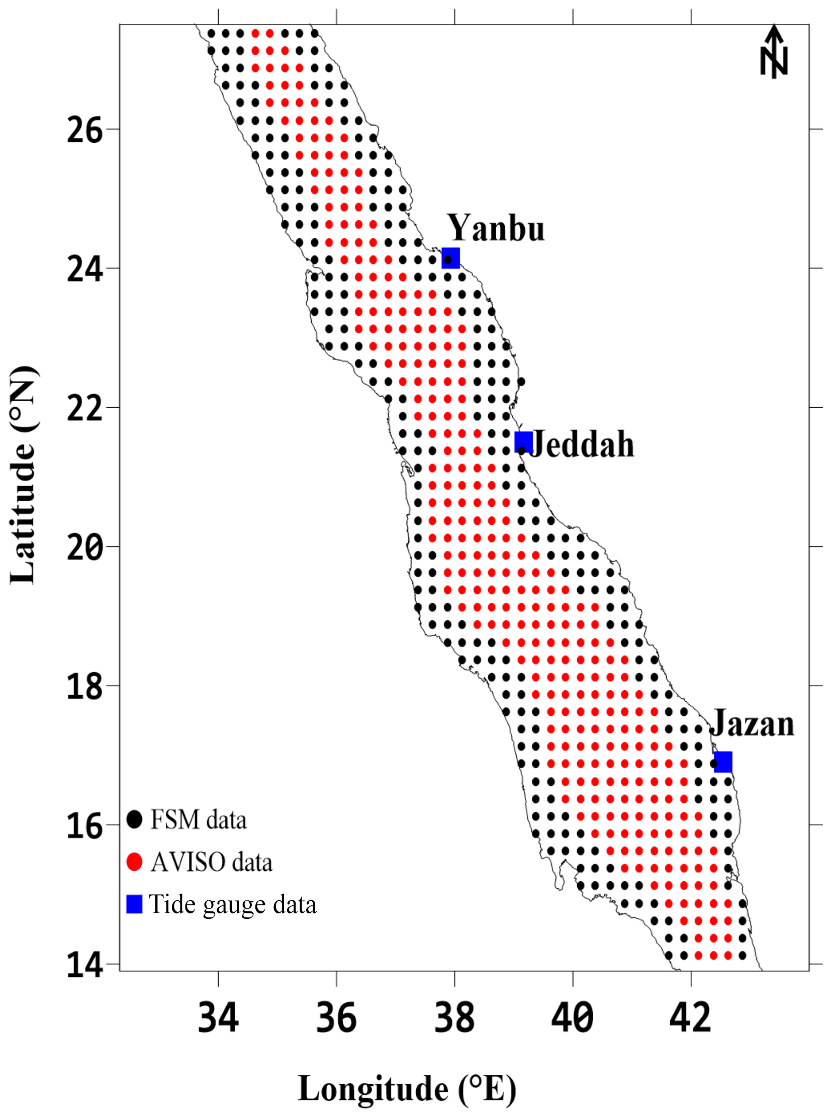
Figure 1 The study area, the grid-point locations with a spatial resolution of $\mathrm{0.25}{}^{\circ }\times {\mathrm{0.25}}^{\circ }$, and locations of the tide gauges.

In recent years, there has been increasing interest in using satellite altimetry, which offers large coverage and long-data-period SSH (hence sea level anomaly – SLA), wave height, and wind speed (Chelton et al., 2001). However, the altimeter data undergo several processing stages for corrections due to atmosphere and ocean effects (Chelton et al., 2001). The satellite altimetric data have been used for the open ocean for a long time with great success, while the data from the coastal region suffer from gaps of almost 50 km from the coastline. The coastal region requires further corrections due to additional difficulties based on the closeness of the land (Deng et al., 2001; Vignudelli et al., 2005; Desportes et al., 2007; Durand et al., 2009; Birol et al., 2010). In the past 2 decades, many researchers have sought to develop different methods to improve the quality, accuracy, and availability of altimetric data near the coast (e.g., Vignudelli et al., 2000; Deng and Featherstone, 2006; Hwang et al., 2006; Guo et al., 2009, 2010; Vignudelli et al., 2005; Desportes et al., 2007; Durand et al., 2009; Birol et al., 2010; Khaki et al., 2014; Ghosh et al., 2015; Taqi et al., 2017). Satellite altimetry faces three types of problems near the coast: (1) echo interference with the surrounding ground as well as inland water surface reflection (Andersen and Knudsen, 2000; Mantripp, 1966), (2) environmental and geophysical corrections such as dry tropospheric correction, wave height, and high-frequency and tidal corrections from global models, and (3) spatial and temporal corrections during sampling (Birol et al., 2010).

Figure 2 The correlation coefficient between AVISO and FSM data.

Figure 3 Comparison of SLA from three tide gauges (black), with grid FSM–SLA data (red) and AVISO (blue).

The ocean currents advect water worldwide. They have a significant influence on the transfer of energy and moisture between the ocean and the atmosphere. Ocean currents play a significant role in climate change in general. In addition, they contribute to the distribution of hydrological characteristics, nutrients, contaminants, and other dissolved materials between the coastal and the open areas and among the adjacent coastal regions. Ocean currents carry sediment from and to the coasts, so they play a significant role in shaping the coasts. That is important in densely inhabited coastal regions producing large amounts of pollutants. Understanding the currents helps us in dealing with the pollutants and coastal management.

The objective of the present research is to study the geostrophic current in the Red Sea, including the coastal region, using modified along-track Jason-2 SLA along the coast produced by Taqi et al. (2017).

2 Material and methods

2.1 Description of data

2.1.1 Fourier series model (FSM) SLA

The SLA data used in this study are weekly Jason-2 altimetry along the track from June 2009 (cycle 33) to December 2014 (cycle 239), which have been extended to the coastal region by Taqi et al. (2017). The extended data show a good agreement with the coastal tide gauge station data. In brief, the FSM method of extending SLA consists of four steps: the first step is the removal from SLA of outliers that are more than 3 times the standard deviation from the mean. In the second step the SLA is recomputed using a Fourier series equation along the track. In the third step the data are then filtered to remove the outliers in the SLA with time, similar to the first step. Finally, the SLA data are linearly interpolated over time to form the new extended data, which are called FSM. For more details on the FSM method, refer to Taqi et al. (2017).

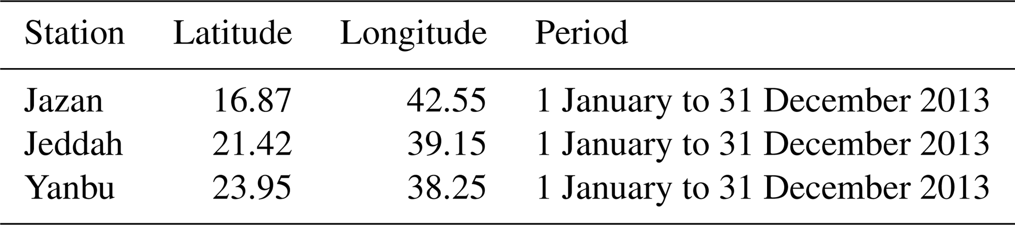
Table 1 The location of tide gauge stations and period of measurement.

2.1.2 AVISO, tide gauge, and hydrographic datasets

This study uses two types of SLA data: the first set is the SLA downloaded from the Archiving Validation and Interpretation of Satellite Oceanographic (AVISO) (http://marine.copernicus.eu/services-portfolio/access-to-products/, last access: 27 November 2015). The second dataset is the SLA from the extended FSM data. The temperature and salinity profiles used for geostrophic estimation are received from three cruises: the first cruise was during 16 to 29 March 2010 onboard R/V Aegaeo between 22 and 28^∘ N along the eastern Red Sea with a total of 111 conductivity, temperature, and depth (CTD) profiles. For more details, see Bower and Farrar (2015). The second cruise was from 3 to 7 April 2011 onboard Poseidon between 17 and 22^∘ N in the central eastern Red Sea, and the third one was during 16 to 19 October 2011 onboard the same vessel between 19 and 23^∘ N in the central eastern Red Sea as a part of the Jeddah transect for the KAU-KEIL project. For more details, consult R/V Poseidon cruise P408/1 report (Schmidt et al., 2011). The availability of in situ observations is limited in space and time because of the spatial and temporal distribution of the available cruises. Finally, data from three tide gauges at the eastern coastline of the Red Sea are obtained from the General Commission of Survey (SGS) of the Kingdom of Saudi Arabia (Fig. 1), and their location details are shown in Table 1.

Table 2 Statistical analysis for AVISO and FSM–SLA data comparison with observed coastal tide gauge data (in 2013).

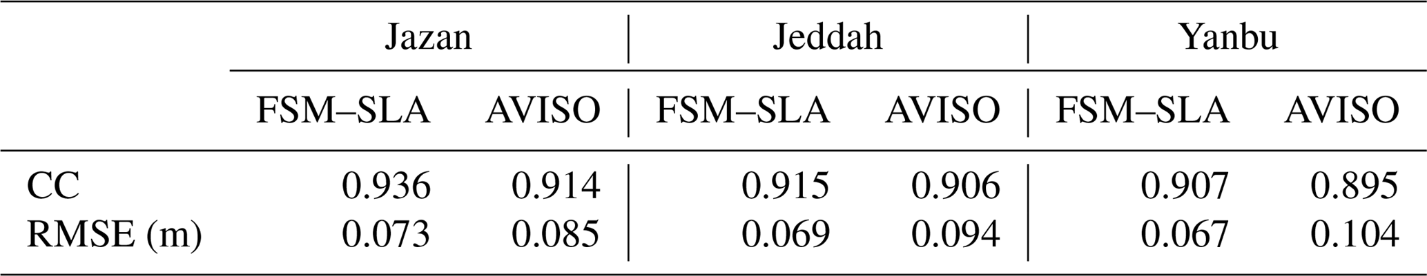
Note: the p value corresponding to all comparisons is very low (P < 0.0001), indicating that the results from correlation are significant.

2.2 Method

The SLA data used in this study come from two sources: (1) the FSM data near the coast and (2) the AVISO data along the axis of the Red Sea. The steps to merge the two datasets and calculate the geostrophic currents are given below.

First, the along-track FSM data are used to produce gridded data to a spatial resolution of $\mathrm{0.25}{}^{\circ }\times \mathrm{0.25}{}^{\circ }$ for comparison with AVISO data. In the second step, AVISO data near the coast are removed and replaced with the coastal FSM gridded data, leaving space between the two datasets according to the width of the sea: either one or two grid cells. This gap was filled using interpolation (kriging) to smooth the dataset. The merged data are hereafter referred to as FSM–SLA. Finally, surface geostrophic currents are estimated from FSM–SLA data using the following equation:

$$\begin{array}{}\text{(1)}& {\displaystyle }{u}_{\mathrm{g}}=-{\displaystyle \frac{g}{f}}{\displaystyle \frac{\partial \mathit{\zeta }}{\partial y}}{v}_{\mathrm{g}}={\displaystyle \frac{g}{f}}{\displaystyle \frac{\partial \mathit{\zeta }}{\partial x}},\end{array}$$

where (u_g, v_g) is the surface geostrophic current, g is gravity, f is the Coriolis parameter, and ζ is the sea surface height. The estimation of geostrophic currents from CTD data uses the following equation:

$$\begin{array}{}\text{(2)}& {\displaystyle }{u}_{\mathrm{g}}=-{\displaystyle \frac{\mathrm{1}}{f\mathit{\rho }}}{\displaystyle \frac{\partial p}{\partial y}}{v}_{\mathrm{g}}={\displaystyle \frac{\mathrm{1}}{f\mathit{\rho }}}{\displaystyle \frac{\partial p}{\partial x}},\end{array}$$

where ρ is the density of seawater, and p is hydrostatic pressure derived from the density. The stations have depths that vary from 50 to 2344 m. However, most of the stations (∼90 %) exceed 500 m of depth. A previous study by Quadfasel and Baudner (1993) used 400 m as the level of no motion to calculate geostrophic current in the Red Sea. Based on acoustic Doppler current profiler (ADCP) measurements, Bower and Farrar (2015) showed that, on average, 75 %–95 % of the vertical shear occurred over the top 200 m of the water column. Moreover, the ADCP measurements of current speed below 500 m are very small: about ∼0.06 m s⁻¹ at 600 m of depth (Bower and Farrar, 2015). Therefore, expecting negligible variability below 500 m, a depth of 500 m was selected as a level of no motion. We have compared the geostrophic current corresponding to levels of no motion at 500 and 700 m. The observed difference between the two is negligibly small, with a root mean square error (RMSE) around 0.003 m s⁻¹ at the surface.

Figure 4 Comparison for 3-month SLA (color) and geostrophic currents (black vectors) between (a, c, e) AVISO and (b, d, f) FSM–SLA. Red vectors show geostrophic currents from CTD data.

3 Results and discussion

3.1 Validation of FSM–SLA and geostrophic current

Statistical analysis has been conducted to show the quality of FSM–SLA compared with AVISO. The correlation coefficient (CC) reveals a good agreement between the two datasets in the open sea (about 0.7 to 0.9) and is shown in Fig. 2. In contrast, near the coasts, weak correlation is found between the two datasets, with the correlation coefficient being 0.45 to 0.7.

Furthermore, the observed SLA from the coastal tide gauge is compared with the FSM–SLA data and AVISO datasets. Table 2 illustrates some of the statistical analysis; the RMSE is less for FSM–SLA compared to that of AVISO.

Figure 3 shows the SLA time series for 2013 from the three coastal stations compared with FSM–SLA and AVISO. The three station datasets have similar seasonal patterns, and FSM–SLA coincides with observed SLA in shorter-duration fluctuations. The comparison of FSM–SLA data and the observed SLA data (at Jazan, Jeddah, and Yanbu stations) shows a better correlation than between the AVISO and observed SLA data as shown in Fig. 3 and Table 2. These correlation coefficient differences indicate that FSM–SLA shows better accuracy near the coast. These results were consistent with those obtained for along-track Jason-2 SLA compared with coastal stations by Taqi et al. (2017).

Figure 4 shows a comparison between the geostrophic currents for the central Red Sea derived from AVISO and FSM–SLA for three different times (March 2010, April and October 2011) corresponding to the timing of the three cruises described in Sect. 2.1.

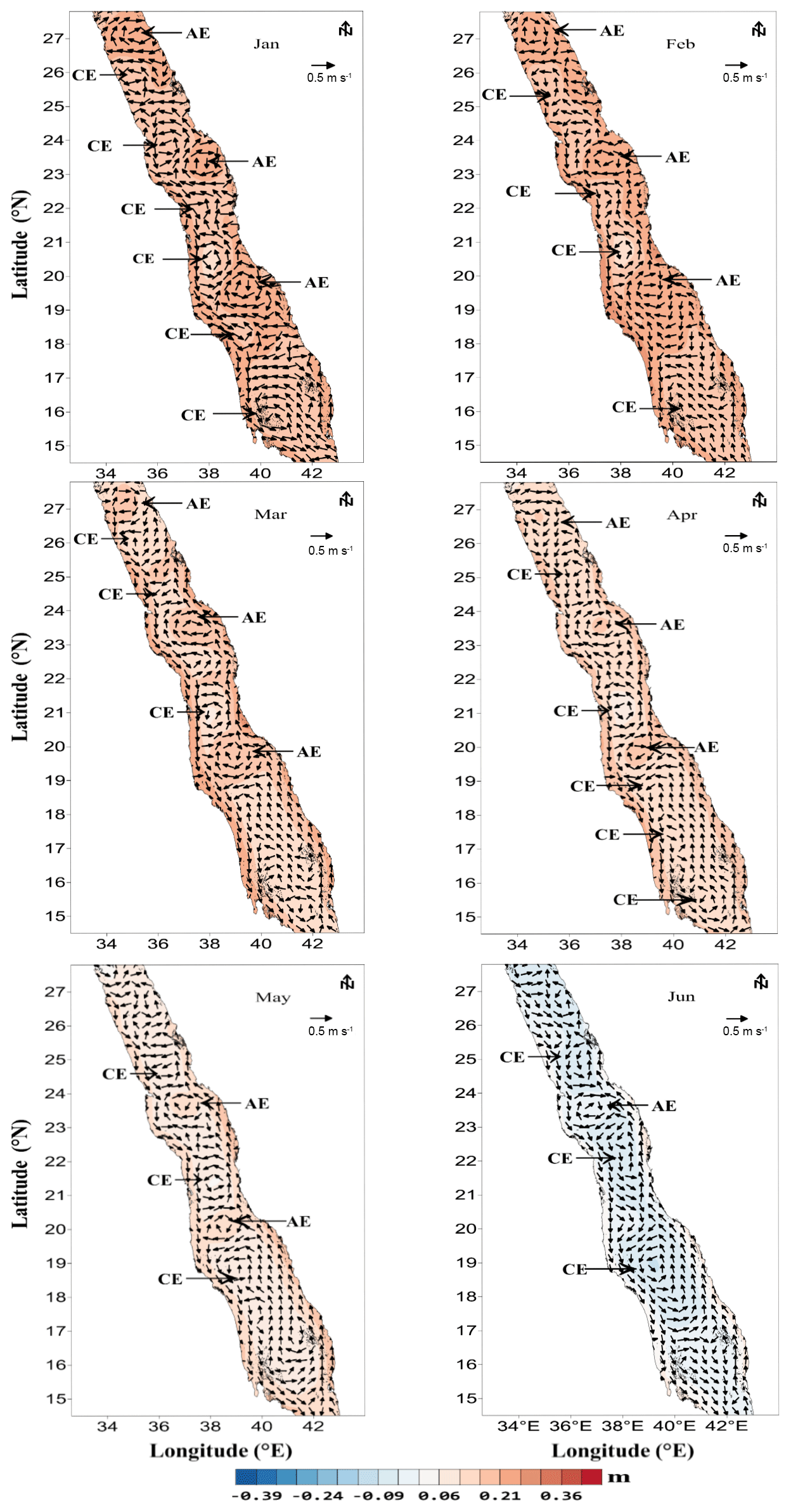
Figure 5 Monthly climatology for geostrophic current and sea level anomaly (reference current length:  0.5 m s⁻¹).

Figure 6 As Fig. 5 for July to December.

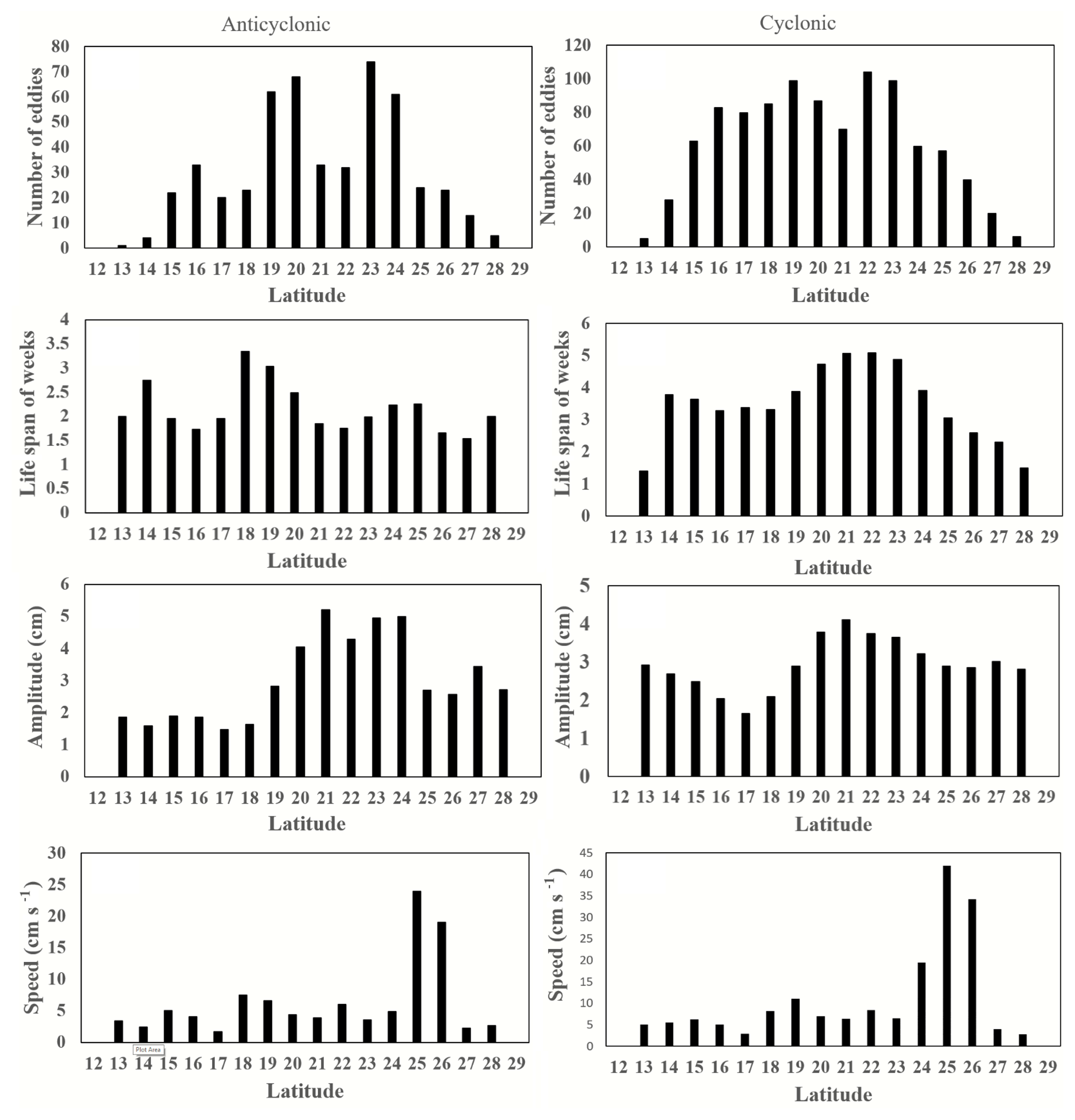
Figure 7 The variability with latitude for cyclonic (right panels) and anticyclonic eddies (left panels).

It can be seen from the Fig. 4b, d, and f that there is a significant match in the directions of geostrophic currents from FSM–SLA with geostrophic currents from CTD data near the coast and offshore. This result is in agreement with the Bower and Farrar (2015) findings, especially in October 2011 (Fig. 4f). In March 2010, the geostrophic current near the coast estimated from FSM–SLA matches the directions of CTD-derived geostrophic currents in most regions. However, the directions of geostrophic currents from AVISO do not always match CTD-derived currents, especially in October 2011.

In March 2010 the geostrophic currents along the eastern coast of the Red Sea are towards the north for both FSM–SLA and AVISO, except between 22.2 and 23^∘ N, where the FSM–SLA and CTD data geostrophic currents are in the same direction, while the AVISO geostrophic current is in the opposite direction (see Fig. 4a, b).

The speed of geostrophic currents derived from FSM–SLA and CTD during the months of March 2010 and April and October 2011 shows a stronger correlation compared with the speed of geostrophic currents derived from AVISO and CTD as shown in Fig. 4 and Table 3.

3.2 Description of FSM–SLA and geostrophic current

Figure 5 shows monthly climatology variation for the 5.5-year period for SLA and geostrophic current. The SLA is higher during the period from October to May and lower during rest of the year; this pattern is consistent with previous studies (Patzert, 1974; Edwards, 1987; Ahmad and Sultan, 1989; Sofianos and Johns, 2001; Sultan and Elghribi, 2003; Manasrah et al., 2004, 2009). Based on calculations made here, the geostrophic current along the eastern coast of the Red Sea is northward, while along the western coast it is southward. This northward-flowing current is consistent with a previous study by Bower and Farrar (2015). Similar results are also obtained from three-dimensional modeling by Clifford et al. (1997), Eshel and Naik (1997), and Sofianos and Johns (2002, 2003).

Figure 5 presents the surface circulation during January in the northern part, where two eddies formed between 25 and 27.5^∘ N. The first eddy is an anticyclone between 26.3 and 27.5^∘ N on the eastern side of the Red Sea. The other eddy is cyclonic and located between 25 and 26.3^∘ N near the western coast. To the south of that, there are two other eddies between 22.5 and 24.7^∘ N: cyclonic on the western side and anticyclonic on the eastern side. These results match those observed in previous studies (Eladawy et al., 2017; Sofianos and Johns, 2002, 2003). Two cyclonic eddies and an anticyclonic eddy found at 19.5 and 22.5^∘ N are consistent with those modeled by Sofianos and Johns (2003). Near Bāb al Mandab, there is a cyclonic eddy on the western side between 15 and 16.5^∘ N.

In February, the surface circulation of the Red Sea is similar to that during January, with some differences in the eddy structure. The anticyclonic eddy near 27^∘ N on the eastern side of the Red Sea starts shifting toward the western coast, while a cyclonic eddy at 25–26.3^∘ N starts appearing. The cyclonic eddies between 22.5 and 24.7^∘ N on the western side are less clear in this month.

In March and April, all the eddies are located along the central axis of the Red Sea. In the north, the anticyclonic eddy near 27^∘ N is shown in both months, while the cyclonic eddy is not clear during March and April. The anticyclonic eddy shown near 23–24^∘ N during March is weakening during April. Also, the anticyclonic eddy between 19 and 20^∘ N is shrinking during April.

Figure 8 Maps of the annual mean SLA as a deviation from the 5.5-year mean.

In May, there is no clear eddy between 25 and 27.5^∘ N. However, four eddies clearly exist between 19.5 and 25^∘ N: two cyclonic eddies at 24–25 and 20–22^∘ N and two anticyclonic eddies at 23–24 and 19.5–20^∘ N. From the previous results, it can be seen that several cyclonic and anticyclonic eddies are distributed all over the Red Sea and these results match those in modeling studies (Clifford et al., 1997; Eladawy et al., 2017; Sofianos and Johns, 2002, 2003, Yao et al., 2014a)

During June, the geostrophic currents in the northern part reversed their direction. This accompanies the formation of a large cyclonic eddy extending from 25.5 to 27.5^∘ N and occupying the entire width of the Red Sea. To the south of it, another cyclonic eddy observed between 24 and 25^∘ N and an anticyclonic eddy between 23 and 24^∘ N are also observed during June with a similar strength as in May. The cyclonic eddy seen between 17 and 20^∘ N during May is also seen during this month with more strength. To the south of it, the flow is towards the Bāb al Mandab following the normal summer pattern. The flow pattern along the coast is similar to results of Chen et al. (2014) for winter (January to April). The short-term climatology of geostrophic currents in the Red Sea is dominated by cyclonic and anticyclonic eddies all over the Red Sea, especially in the central and northern parts of the sea.

During July–September, the geostrophic current structure is similar to that of June with two cyclonic eddies north of 24.5^∘ N and an anticyclonic eddy between 23 and 24^∘ N. South of these eddies, another cyclonic eddy extends to 19^∘ N. Furthermore, south of 19^∘ N, there is an outflow towards the south over almost the entire width of the Red Sea with narrow inflow along the eastern coast of the Red Sea. Figure 6 also shows an anticyclone between 18 and 19^∘ N and a cyclone between 16 and 17^∘ N during August and September. These results are consistent with the results from previous studies (Clifford et al., 1997; Eladawy et al., 2017; Sofianos and Johns, 2002, 2003, Yao et al., 2014b).

Table 3 Statistical analysis for the speed of geostrophic current from FSM–SLA and AVISO compared with CTD-derived geostrophic current from the three cruises.

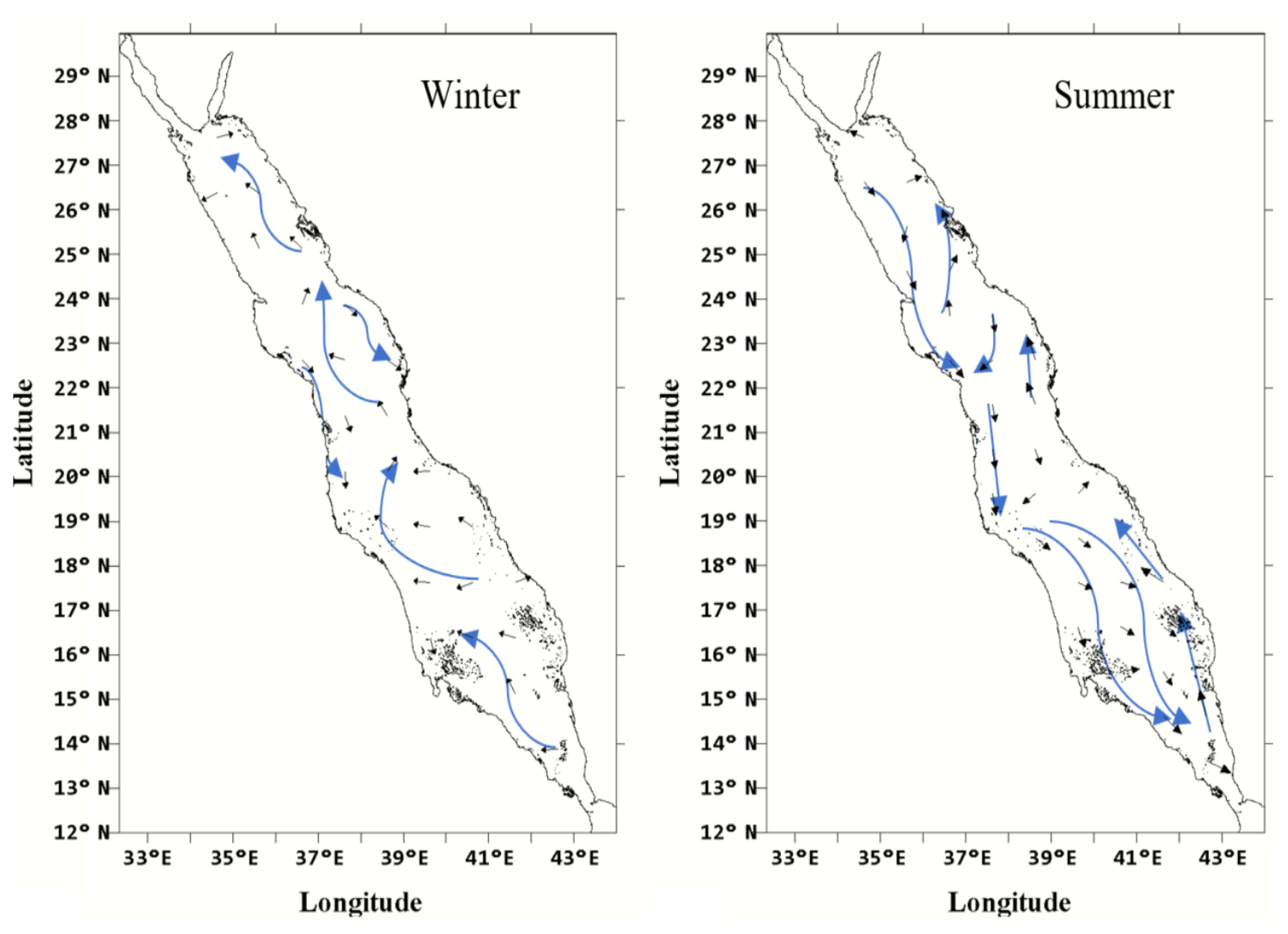
Figure 9 A general schematic of winter and summer seasonal average surface geostrophic currents; black arrows are actual surface geostrophic currents and blue arrows are the schematic streamline.

During summer (June–September), the changes in wind speed and direction cause reversals of the direction of flow. Consequently, the locations of eddies are also changed (Chen et al., 2014). The surface current flows from the Red Sea to the Gulf of Aden through the Bāb al Mandab. The anticyclonic eddy shown in the north at 27.5^∘ N in winter is replaced with a cyclonic eddy during this season. Summer is dominated by cyclonic eddies as shown in Fig. 6.

During October, the geostrophic current is weak compared with that during September, still cyclonic but with less strength. The anticyclone seen during September between 23 and 24^∘ N is not clear during October, but an anticyclonic eddy forms between 15 and 16^∘ N. In the central and southern parts, the flow of the geostrophic currents is towards the south along the western coast and towards the north along the eastern side with the presence of cyclonic and anticyclonic eddies in the central axis of the Red Sea with a weak flow. In November and December, the structure of geostrophic currents is similar to that of October but with stronger currents and well-established cyclonic and anticyclonic eddies.

During early summer the eddies are concentrated along the central Red Sea. By August and September some of the cyclonic eddies are shifted towards the eastern coast. During winter the cyclonic eddies are often condensed along the western side of the Red Sea, with anticyclonic eddies along the eastern side of the Red Sea. Their formation might be related to wind and thermohaline forces (Neumann and McGill, 1961; Phillips, 1966; Quadfasel and Baudner, 1993; Siedler, 1969; Tragou and Garrett, 1997).

Table 4 Statistical analysis of the annual mean of FSM–SLA from the climatology.

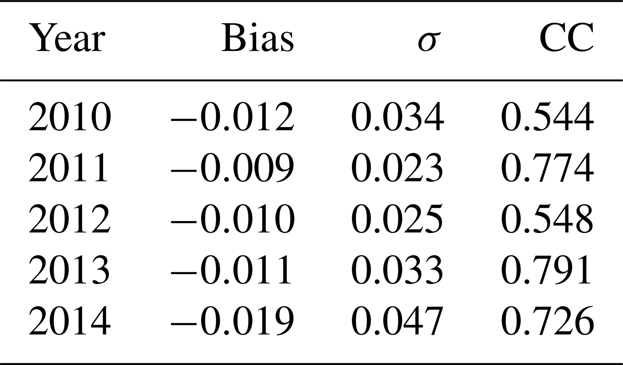
Note: the p value corresponding to all comparisons is very low (P < 0.0001), indicating that the results from correlation are significant.

To conform that the above variation is due to month-to-month variation and not due to variation between the same months from different years used for the climatology, a standard deviation between the monthly climatology and the months used to create the climatology is estimated. The result shows a small standard deviation all over the Red Sea for all the months. The highest standard deviation is seen during the months of April, October, and November with 0.232, 0.209, and 0.241, respectively, in the northern part along the coast. The lowest standard deviation is seen during March, October, and December with 0.008, 0.007, 0.009, respectively, in the southern part of the Red Sea. The southern part of the Red Sea shows a smaller standard deviation than the northern part (Fig. S1, Table S1). The annual mean standard deviation is about 0.057.

Since the general circulation in the Red Sea is largely modified by the presence of cyclonic and anticyclonic eddies, the identification of eddies in the study area was conducted based on defining the eddies in terms of SLA (Chelton et al., 2011). Figure 7 shows the statistical variability of life span, number of eddies, amplitude, and the mean speed of geostrophic currents in the center of the eddies with latitude for 5.5 years. Statistical analysis indicates that eddies are generated over the entire Red Sea, mostly concentrated between 18 and 24^∘ N and obviously stronger than at other latitudes. The amplitude of an eddy has been defined as the difference between the estimated basic height of the eddy boundary and the extremum value of SLA inside the eddy interior. The mean amplitude for an anticyclonic eddy is 1.3 cm in the southern Red Sea and 5.3 cm in the northern Red Sea, and for a cyclonic eddy it is 1.6 cm in the southern Red Sea and 4.2 cm in the northern Red Sea. The result indicates that the average value of eddy amplitude in the Red Sea (including low latitudes and high latitudes) is about 2.96 cm, which is within the reasonable range defined by Chelton et al. (2011). The average life span of the cyclonic eddies is longer than that of the anticyclonic eddies. Moreover, the mean speed of a geostrophic current for the entire Red Sea is about 5–10 cm s⁻¹, but it is 3 times greater in the 25 and 26^∘ N latitude band for both cyclonic and anticyclonic eddies. These results match those observed in a previous study by Zhan et at. (2014).

Figure 8 shows the annual mean of SLA as a deviation from the 5.5-year mean. The interannual variability of SLA and geostrophic currents is clearly seen in the southern part of the Red Sea, while in the northern part, the pattern is similar for all years except for 2013 when the cyclonic eddy is replaced by anticyclonic eddy. The SLA and geostrophic distribution observed during 2011 are similar to that shown in Papadopoulos et al. (2015), with the cyclonic eddy along the eastern side seen more clearly. Moreover, due to the extension of our data we could compute the cyclonic pattern up to the coast. The geostrophic current direction is irregular along the coast but is northward most of the time. The eddies were mostly concentrated in the north and central parts of the Red Sea.

The statistical analysis of annual FSM–SLA with 5.5-year climatology is shown in Table 4. The correlation is significant for all the years with a standard deviation (σ) less than 0.1. The bias is very small regardless of its sign.

Figure 9 shows the general schematic of the seasonal variability of geostrophic currents derived from 5.5 years. During winter, the mean flow is toward the north over most of the width of the Red Sea; this result agrees with Sofianos and Johns (2003). In addition, southward geostrophic currents were observed along the eastern coast at 22–24^∘ N and the western coast at 23–20^∘ N. During summer, the flow is towards the south along the western side of the sea, while in the southern part the flow spreads across most of the width of the Red Sea with a narrow northward flow near the eastern coast.

4 Conclusions

In general, the geostrophic current has been estimated from FSM–SLA for the Red Sea region, and the distribution of the geostrophic current shows that the winter period extends from October to May and summer period extends from June to September. This pattern is similar to that shown by Sofianos and Johns (2001). There was a lack of measurements for coastal currents in the Red Sea. This study was able to produce data near the coast. The major new findings from the present study include the monthly geostrophic pattern in the Red Sea, which has not been published before.

The southern Red Sea shows significant interannual variability in the geostrophic current pattern, while the central and northern parts show a negligible difference over the years. The geostrophic current along the eastern coast is towards the north, while along the western coast of the sea it is southward. Seasonally, the geostrophic currents in summer flow southward except along the eastern coast where they flow in the opposite direction. In winter, currents flow to the north for the entire sea except for a southward flow along a small part of the eastern (22–24^∘ N) and western coast (20–23^∘ N). In this study, a northward-flowing eastern coastal current during summer is documented for the first time in the Red Sea.

Cyclonic eddies were relatively larger than anticyclonic eddies in the Red Sea. The eddies are concentrated in the central and northern Red Sea more than in the southern part. Anticyclonic and cyclonic eddies at lower latitudes have small amplitude and at higher latitudes have a larger mean amplitude. In winter, the cyclonic eddies are beside the western coast and anticyclonic eddies on the eastern side in the Red Sea, while in summer they are concentrated along the central Red Sea in early summer, with some cyclonic eddies transferring to the east coast in late summer. Also, in some locations there is a noticeable change from anticyclonic during winter to cyclonic during summer and vice versa between 26.3 and 27.5^∘ N. During the summer the cyclonic eddies are dominant in the entire Red Sea, while eddies of both polarities were observed during winter. The finding of this paper is considered the first of its type in the Red Sea for extending SLA and geostrophic currents to the coast in addition to giving more details on eddy spatial and temporal variabilities in the coastal region.