Hybrid improved empirical mode decomposition and BP neural network model for the prediction of sea surface temperature

Sea surface temperature (SST) is the major factor that affects the ocean–atmosphere interaction, and in turn the accurate prediction of SST is the key to ocean dynamic prediction. In this paper, an SST-predicting method based on empirical mode decomposition (EMD) algorithms and back-propagation neural network (BPNN) is proposed. Two different EMD algorithms have been applied extensively for analyzing time-series SST data and some nonlinear stochastic signals. The ensemble empirical mode decomposition (EEMD) algorithm and complementary ensemble empirical mode decomposition (CEEMD) algorithm are two improved algorithms of EMD, which can effectively handle the mode-mixing problem and decompose the original data into more stationary signals with different frequencies. Each intrinsic mode function (IMF) has been taken as input data to the back-propagation neural network model. The final predicted SST data are obtained by aggregating the predicted data of individual series of IMFs (IMFi). A case study of the monthly mean SST anomaly (SSTA) in the northeastern region of the North Pacific shows that the proposed hybrid CEEMD-BPNN model is much more accurate than the hybrid EEMD-BPNN model, and the prediction accuracy based on a BP neural network is improved by the CEEMD method. Statistical analysis of the case study demonstrates that applying the proposed hybrid CEEMD-BPNN model is effective for the SST prediction. Highlights include the following:

Highlights.

• An SST-predicting method based on the hybrid EMD algorithms and BP neural network method is proposed in this paper.

• SST prediction results based on the hybrid EEMD-BPNN and CEEMD-BPNN models are compared and discussed.

• A case study of SST in the North Pacific shows that the proposed hybrid CEEMD-BPNN model can effectively predict the time-series SST.

1 Introduction

Sea surface temperature (SST) is a main factor in the interaction between the ocean and the atmosphere (Wiedermann et al., 2017; He et al., 2017; Wu et al., 2019a), and it characterizes the combined results of ocean heat (Buckley et al., 2014; Griffies et al., 2015; Wu et al., 2019b) and dynamic processes (Takakura et al., 2018). It is a very important parameter for climate change and ocean dynamics processes, such as sea–air heat fluxes and water vapor exchange. Small changes in sea temperature can have a huge impact on the global climate. The well-known El Niño and La Niña phenomena are caused by abnormal changes in SST (Z. Chen et al., 2016; Zheng et al., 2016).

Therefore, scholars have begun to observe the SST in recent years; the observation of the SST is important (Kumar et al., 2017; Sukresno et al., 2018). Accurate observation and effective prediction of the SST are very important (Hudson et al., 2010). Predicting the SST in advance can enable people to take appropriate measures to reduce the impact on daily life and reduce unnecessary losses. However, due to the high randomness and irregularity of the monthly mean sea surface temperature anomaly (SSTA), the nonlinear and non-stationary characteristics are obvious. At present, there is no clear and feasible method with high accuracy to effectively predict the SST (Zhu et al., 2015; C. Chen et al., 2016; Khan et al., 2017).

In mathematics and science, a nonlinear system is a system in which the change of the output is not proportional to the change of the input. Nonlinear dynamical systems, describing changes in variables over time, may appear chaotic, unpredictable, or counterintuitive, contrasting with much simpler linear systems. A stationary process is a stochastic process whose unconditional joint probability distribution does not change when shifted in time. Consequently, statistical parameters such as mean and variance also do not change over time. The variation of SST is a nonlinear dynamic system with non-stationary time-series data. Empirical mode decomposition (EMD) is a state-of-the-art signal-processing method proposed by Huang et al. (1998). This method can decompose the signal data of different frequencies step by step according to the characteristics of the data and obtain several orthogonal components and a trending component (W. Wang et al., 2015; Amezquita-Sanchez and Adeli, 2015; Wang et al., 2016; Kim et al., 2016). The EMD method is powerful and adaptive in analyzing nonlinear and non-stationary datasets. It provides an effective approach for decomposing a signal into a collection of so-called intrinsic mode functions (IMFs), which can be treated as empirical basis functions (Duan et al., 2016b). However, there were some problems with the EMD method, such as mode mixing (Huang and Wu, 2008; Wu et al., 2008; Wu and Huang, 2009).

Once an intermittent signal appears in the actual signal, the EMD decomposition method will produce a mode mixing problem. The mode mixing problem causes the essential modal functions (IMFs) to lose their physical meaning. The problem is manifested as either a single IMF consisting of widely disparate scales or a signal of similar scale captured in different IMFs. To overcome mode mixing, two noise-assisted methods have emerged.

Wu and Huang (2009) proposed the ensemble empirical mode decomposition (EEMD) method by adding different white noise in each ensemble member to suppress mode mixing. EEMD adds a fixed percentage of white noise to the signal before decomposing it. This step is repeated N times, after which all results are averaged. EEMD improves the mode-mixing problem but it cannot completely reconstruct the input signal from the resulting components.

Yeh et al. (2010) added two opposite-signal white noises to the time-series data sequence and proposed an improved algorithm: complete ensemble empirical mode decomposition (CEEMD). Similarly, the method decomposes the signal with N different noise realizations but here the results are averaged after each IMF is found. The decomposition effect is equivalent to EEMD, and the reconstruction error caused by adding white noise is reduced (Tang et al., 2015). CEEMD solves the mode mixing problem and it provides an exact reconstruction of the input signal. In contrast to the EEMD method, the CEEMD also ensures that the IMF set is quasi-complete and orthogonal. The CEEMD is a computationally expensive algorithm and may take significant time to run. At present, the EMD model and its improved algorithms have been widely used in many fields of ocean science, such as storm surge and sea level rise (Wu et al., 2011; Lee, 2013; Ezer and Atkinson, 2014), tidal amplitude (Cheng et al., 2017; Pan et al., 2018) and wave height (Duan et al., 2016a; Sadeghifar et al., 2017; López et al., 2017). These studies and applications reflected that the EMD model and its improved algorithms can effectively reduce the complexity of the non-stationarity time-series data, which helps further analysis and processing.

For nonlinear prediction, the more commonly used methods are curve fitting (Motulsky and Ransnas, 1987), gray-box model (Pearson and Pottmann, 2000), homogenization function model (Monteiro et al., 2008), neural network (Deo et al., 2001; Y. Wang et al., 2015; Kim et al., 2016) and so on. Among them, the back-propagation neural network (BPNN) (Lee, 2004; Jain and Deo, 2006; Savitha and Mamun, 2017; Wang et al., 2018) has certain advantages in dealing with nonlinear problems; it is a basic machine-learning algorithm and its principle is simple and operability is strong, so it has been widely used in ocean science and engineering.

In view of non-stationary and nonlinear monthly mean SST, the EEMD, CEEMD and BP neural network will be used here to study how to improve the accuracy of SST prediction. The hybrid EMD-BPNN models will be established for the prediction of SSTA in the northeastern region of the Pacific Ocean.

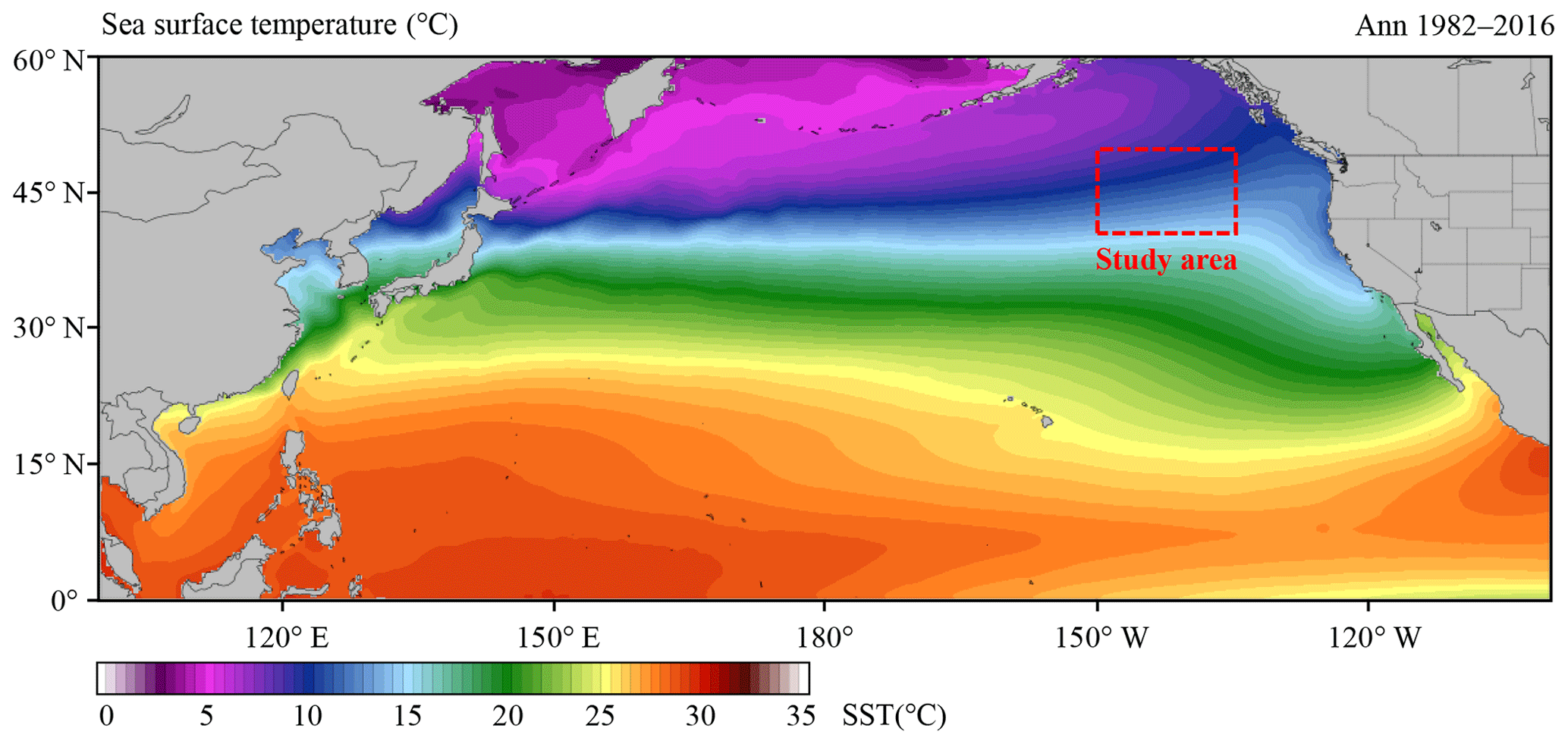
Figure 1 Average sea surface temperature in the North Pacific during January 1982 to December 2016 (35 years).

2 Data collection

SST is the temperature of the top millimeter of the ocean's surface. An anomaly is when something is different from normal, or average. A SSTA shows how different the ocean temperature at a particular location at a particular time is from the normal temperatures for that place. The monthly SSTA is the difference between the SST of this month and the average SST of all instances of this month from 1982 to 2016. The annual SSTA is the difference between the average SST of this year and the average SST of 35 years from 1982 to 2016. For example, a global map of sea surface temperature anomaly for January 2016 would show where the temperatures in January 2016 was warmer, cooler or the same as other January months in previous years. SSTAs can happen as part of normal ocean cycles or they can be a sign of long-term climate change, such as global warming. The SST time-series data in this study are from the National Oceanic and Atmospheric Administration (NOAA) Optimum Interpolation Sea Surface Temperature (OISST) official website (Reynolds et al., 2007; Banzon et al., 2016; https://www.ncdc.noaa.gov/oisst/data-access, last access: March 2017). The NOAA 1∕4^∘ daily OISST is an analysis constructed by combining observations from different platforms (satellites, ships, buoys) on a regular global grid. There are two kinds of OISSTs, named after the relevant satellite SST sensors. These are the Advanced Very High Resolution Radiometer (AVHRR) and Advanced Microwave Scanning Radiometer on the Earth Observing System (AMSR-E); the AVHRR dataset is used in this study. The average annual sea surface temperature in the North Pacific (0–60^∘ N, 100^∘ E–100^∘ W) from January 1982 to December 2016 is shown in Fig. 1.

It has been shown that the sea surface temperature anomaly in the northeastern Pacific in the 10-year period of 2006–2016 was 2.0 ^∘C warmer than in the previous 10 years (1996–2006). Previous studies (Bond et al., 2015) showed that in the spring and summer of 2014, the high SST area of the northeastern Pacific had expanded to coastal ocean waters, which affected the weather in coastal areas and the lives of fishermen, and even affected the temperature in the state of Washington, USA, causing interference to daily life.

In this study, we select the northeastern region of the North Pacific Ocean (in Fig. 1, 40–50^∘ N, 150–135 ^∘W) to measure SST. The time-series data of SST for the study area from January 1982 to December 2016 with a data length of 420 months were obtained from OISST-V2 (Fig. 2). The monthly mean SSTA was used in the analysis and calculation. As shown in Fig. 2a, the overall time-series data are very messy, nonlinear and random from the perspective of the image.

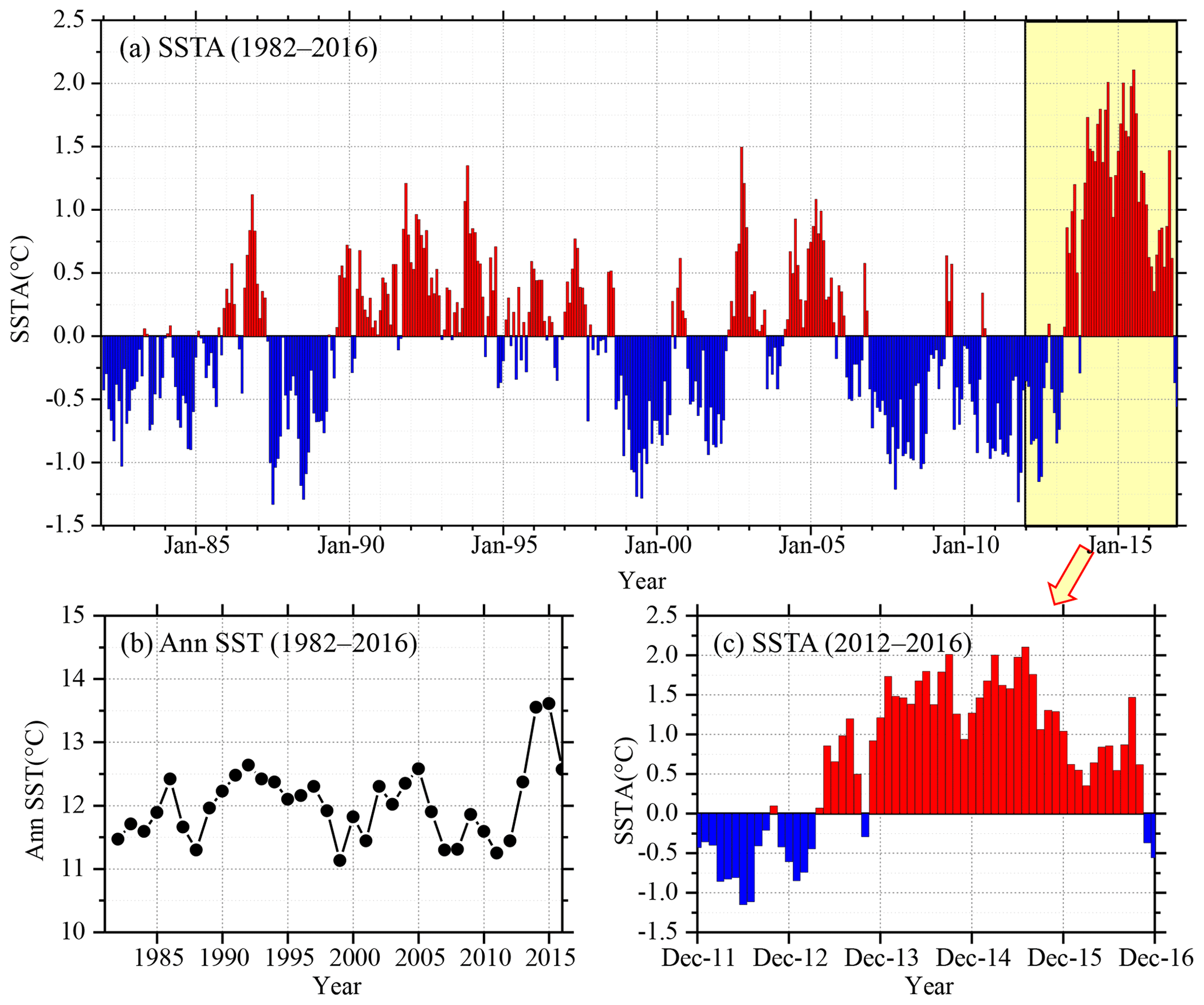
Figure 2 The time-series of sea surface temperature in the study area. (a) SST anomaly (1982–2016; 35 years); (b) annual SST (1982–2016; 35 years); (c) SST anomaly (2012–2016; 5 years).

3 Decomposition of SSTA

The purpose of this study is to combine the EEMD algorithm and the CEEMD decomposition algorithm, respectively, with the BP neural network algorithm to establish a prediction model, a hybrid EMD-BPNN model. The EEMD and CEEMD algorithms are performed on the monthly mean SSTA data to obtain a series of intrinsic mode functions (IMFi). Each IMFi is predicted by a BP neural network and then the IMFi are recombined to obtain the predicted value of SSTA.

3.1 Decomposition by the EEMD algorithm

The SSTA in Fig. 2a has been decomposed based on the EEMD algorithm, and seven IMF components and a residual component (RES; residue) are obtained as shown in Fig. 3.

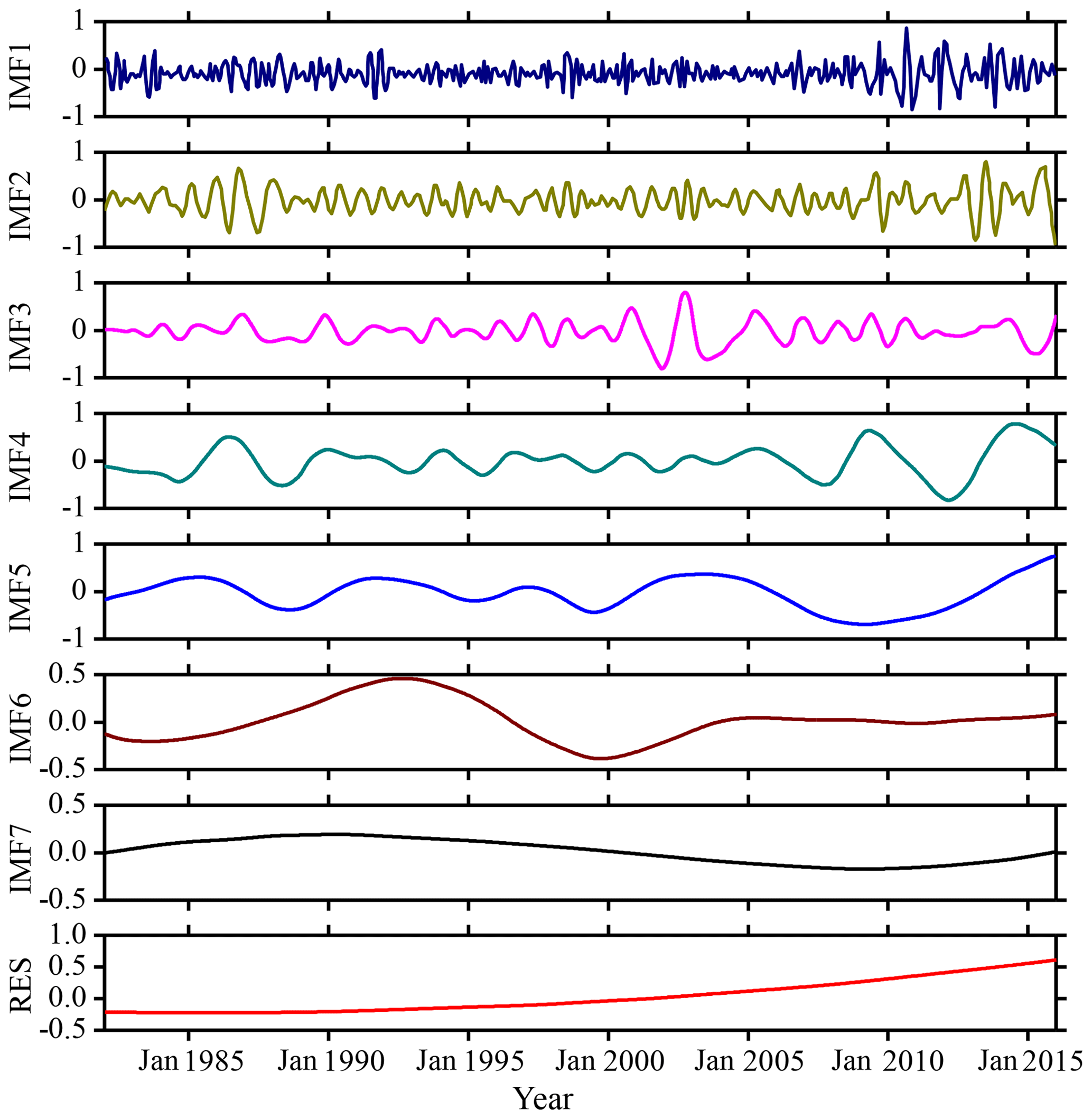
Figure 3 IMF components and the trend item RES of monthly mean SSTA over the study area based on the EEMD algorithm during 1982–2016.

It can be seen from Fig. 3 that the first three intrinsic mode function components (IMF1, IMF2 and IMF3) still exhibit strong non-stationarity because they have strong irregular oscillations and periodic changes. IMF4 to IMF7 and the final trend term (RES) have some periodicity and relatively regular fluctuation, and the non-stationary properties are less than the first three components. The trend term RES reflects that the overall trend of SSTA has gradually increased since 1982. As the non-stationarity of IMFi decreases with increasing i, the EEMD algorithm will reduce the influence of non-stationarity on prediction. The absolute error (ERR) of the decomposition can be calculated by the following equation:

$$\begin{array}{}\text{(1)}& {\displaystyle }{\displaystyle }a\left(t\right)=\left|S\left(t\right)-\left[\sum _{i=\mathrm{1}}^{\mathrm{7}}{I}_i\left(t\right)+R\left(t\right)\right]\right|,\end{array}$$

where a(t) is the ERR, S(t) the original SSTA observation data, I_i(t) the ith component of the IMF (IMF_i), and R(t) the trend term (RES).

The ERR based on the EEMD algorithm is shown in Fig. 4. It can be seen from the figure that the ERR of 420 months after decomposition is basically below 0.01 ^∘C, and the ERR exceeds 0.01 ^∘C in 5 months: June 1989, September 1993, July 1998, May 1999 and March 2010.

In addition to June 1989, the other four monthly data with a large ERR occurred during the El Niño period. The maximum error is in March 2010, the actual value is −0.1204 ^∘C, the result based on EEMD algorithm is −0.1325 ^∘C, the ERR of decomposition is 0.0121 ^∘C; the minimum error, in April 1987, is $\mathrm{1.73}\times {\mathrm{10}}^{-\mathrm{5}}$ ^∘C. The overall mean ERR based on the EEMD algorithm is 0.0035 ^∘C.

Figure 4 The ERR of monthly mean SSTA over the study area based on the EEMD algorithm during 1982–2016.

3.2 Decomposition by the CEEMD algorithm

The SSTA has been decomposed based on the CEEMD algorithm and seven IMF components and a residual component (RES) are obtained as shown in Fig. 5. It can be seen when comparing the decomposition results based on EEMD and CEEMD algorithms that although the mode components decomposed by CEEMD algorithm are different from the corresponding results decomposed by EEMD, the non-stationarities of the seven modes decomposed by the two decomposition algorithms are gradually decreasing, and the final trend term (RES) is an upward trend. Both decomposition algorithms confirm the characteristic of a gradual increase in the overall trend of the data series.

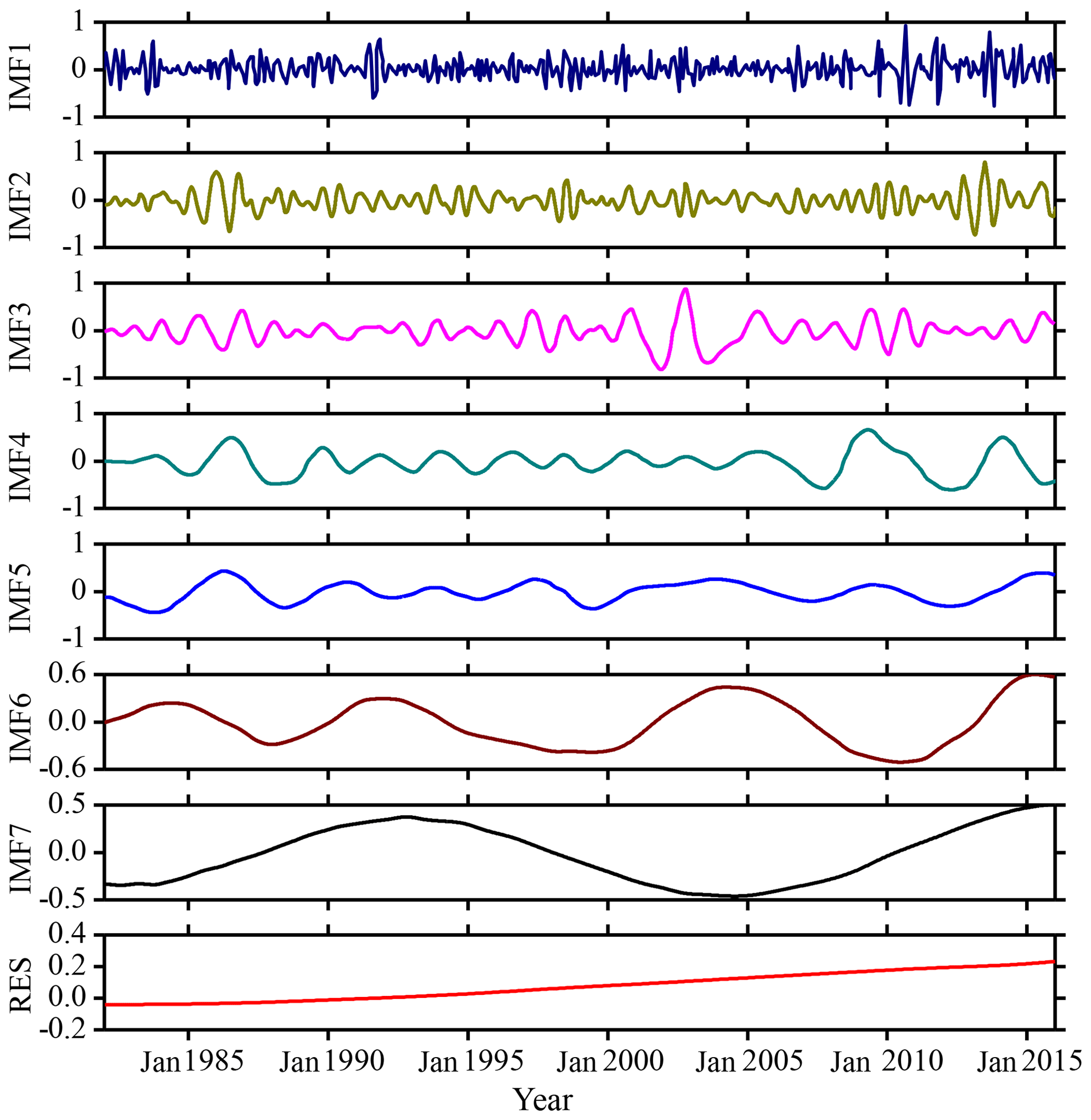
Figure 5 IMF components and the trend item RES of monthly mean SSTA over the study area based on the CEEMD algorithm during 1982–2016.

The ERR obtained based on the CEEMD algorithm is shown in Fig. 6. It can be seen from the figure that the ERR of 420 months of data after decomposition is less than $\mathrm{5}\times {\mathrm{10}}^{-\mathrm{16}}$ ^∘C, and the accuracy is much better. The maximum error is $\mathrm{4.48}\times {\mathrm{10}}^{-\mathrm{16}}$ ^∘C in March 2016; the minimum error is zero. The overall mean ERR based on CEEMD algorithm is $\mathrm{6.10}\times {\mathrm{10}}^{-\mathrm{17}}$ ^∘C. By comparing the results and errors of the above two decomposition algorithms, it can be seen that the error based on the improved algorithm (CEEMD) is much smaller than the error based on the EEMD algorithm. Because more white noise with the opposite sign had been added in the CEEMD algorithm, the reconstruction error caused by the white noise has been reduced compared with that of the EEMD algorithm.

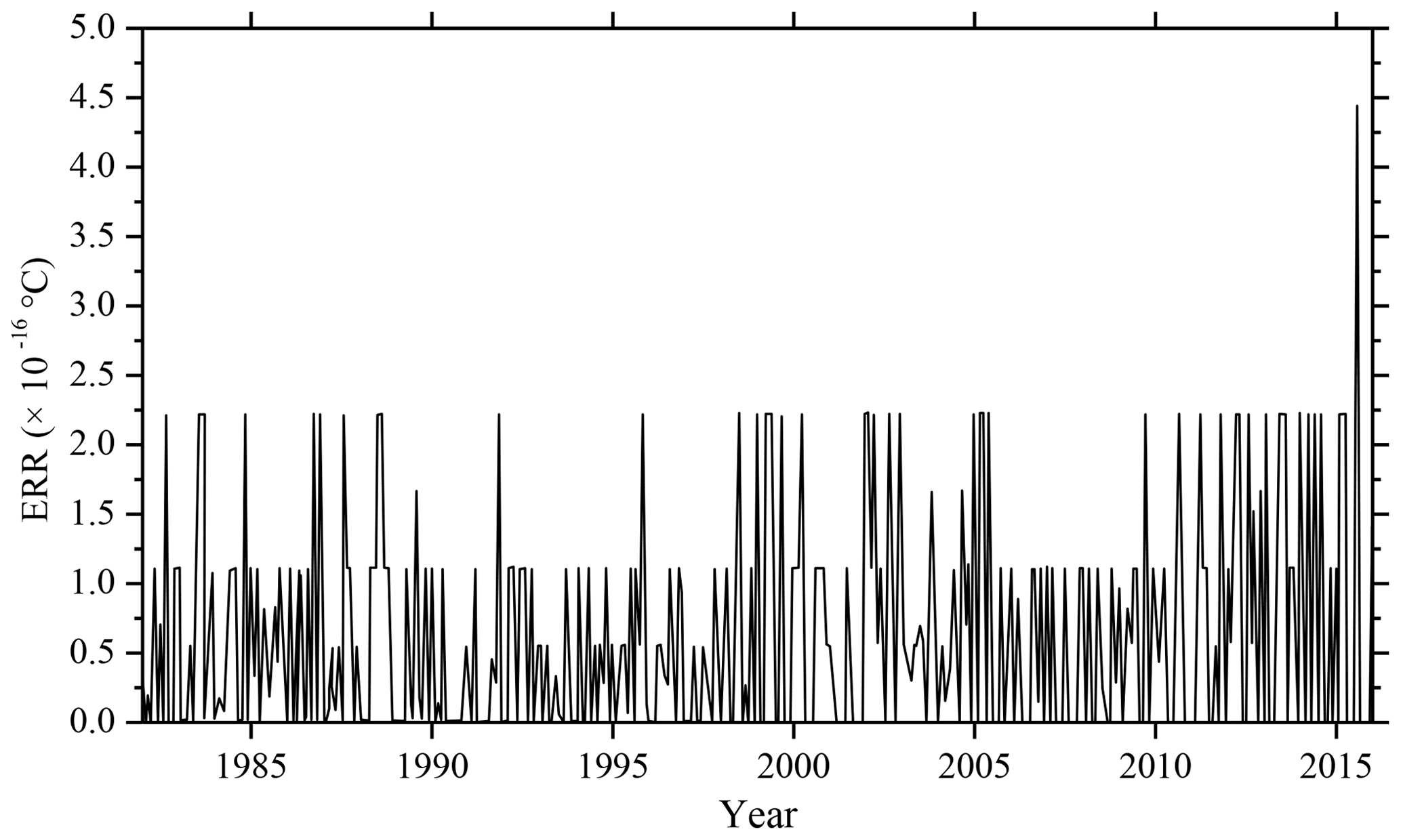
Figure 6 The ERR of monthly mean SSTA over the study area based on the CEEMD algorithm during 1982–2016.

4 SSTA prediction model

4.1 The BP neural network

An artificial neural network (ANN) is an information processing approach based on the biological neural network (López et al., 2017; Kim et al., 2016). In theory, ANN can simulate any complex nonlinear relationship through nonlinear units (neurons) and has been widely used in the prediction area, such as for wave height and storm surge. The most basic structure of ANN consists of input layers, hidden layers and output layers. One of the most widely used ANN models is the BPNN (Wang et al., 2018) algorithm based on the BP algorithm.

The BPNN algorithm is a multi-layer feed-forward network trained according to the error back-propagation algorithm and is one of the most widely used deep learning algorithms. The BP network can be used to learn and store a large number of mappings of input and output models without the need to publicly describe the mathematical equations of these mapping relationships. The learning rule is to use the steepest descent method. When applied to SST prediction, the input data are monthly mean SST in previous months and the output data are predicted SST time-series data. The desired data for comparison are the observed actual SSTs.

4.2 SSTA prediction model based on the hybrid improved EMD-BPNN algorithm

The proposed monthly mean SSTA-predicting model includes three steps as follows. First, original SST datasets are decomposed into certain more stationary signals with different frequencies by EEMD. Second, the BP neural network is used to predict each IMF and the RES. A rolling forecasting process is studied. The prediction is made using the previous data for one step ahead. Finally, the prediction results of each IMF and the RES are aggregated to obtain the final SST prediction results. The flowchart of the SST prediction model based on the hybrid improved empirical mode decomposition algorithm (improved EMD algorithm) and BPNN is shown in Fig. 7. The SST prediction model has been abbreviated as a hybrid improved EMD-BPNN model in the following article.

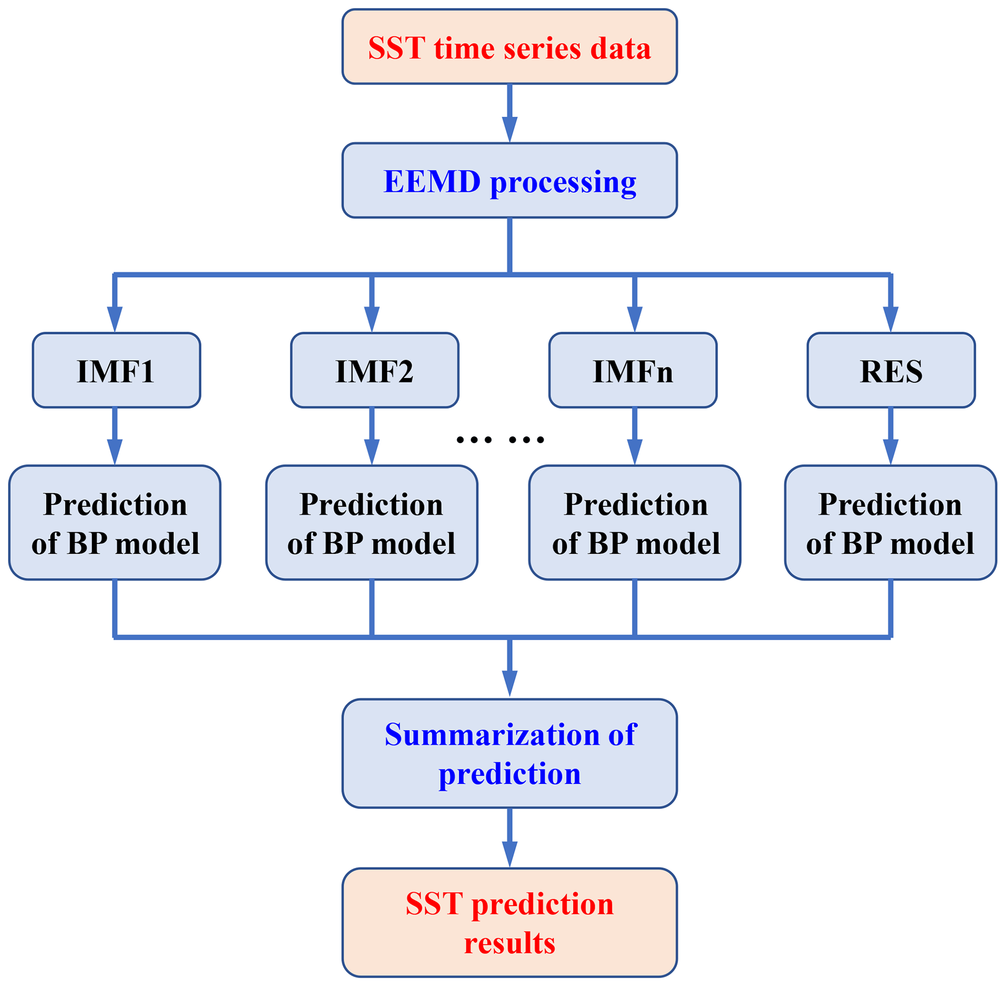
Figure 7 The flowchart of SST prediction model based on the hybrid improved empirical mode decomposition algorithm (improved EMD algorithm) and BPNN.

5 Case study: SSTA prediction based on the hybrid improved EMD-BPNN models

In order to study the effects of the two improved EMD algorithms (EEMD and CEEMD) on the prediction results, and to analyze the prediction ability of BP neural network, the following experiments were carried out: predicting SSTA results in 2017 and analyzing the prediction abilities of different mode decomposition data based on the EEMD and CEEMD algorithms. The experiment content is as follows: the BP neural network is trained with the decomposition data of each mode based on the datasets from 1982 to 2016, and then the SSTA in 2017 is predicted by the trained neural network. The actual results of 12 months in 2017 based on the observation are used to compare and analyze with the prediction results. Time-series SST data from 1982 to 2017 in the study zone are used in this case study, which are decomposed by EEMD and CEEMD into eight different IMFs and the RES as shown in Figs. 8 and 9, respectively.

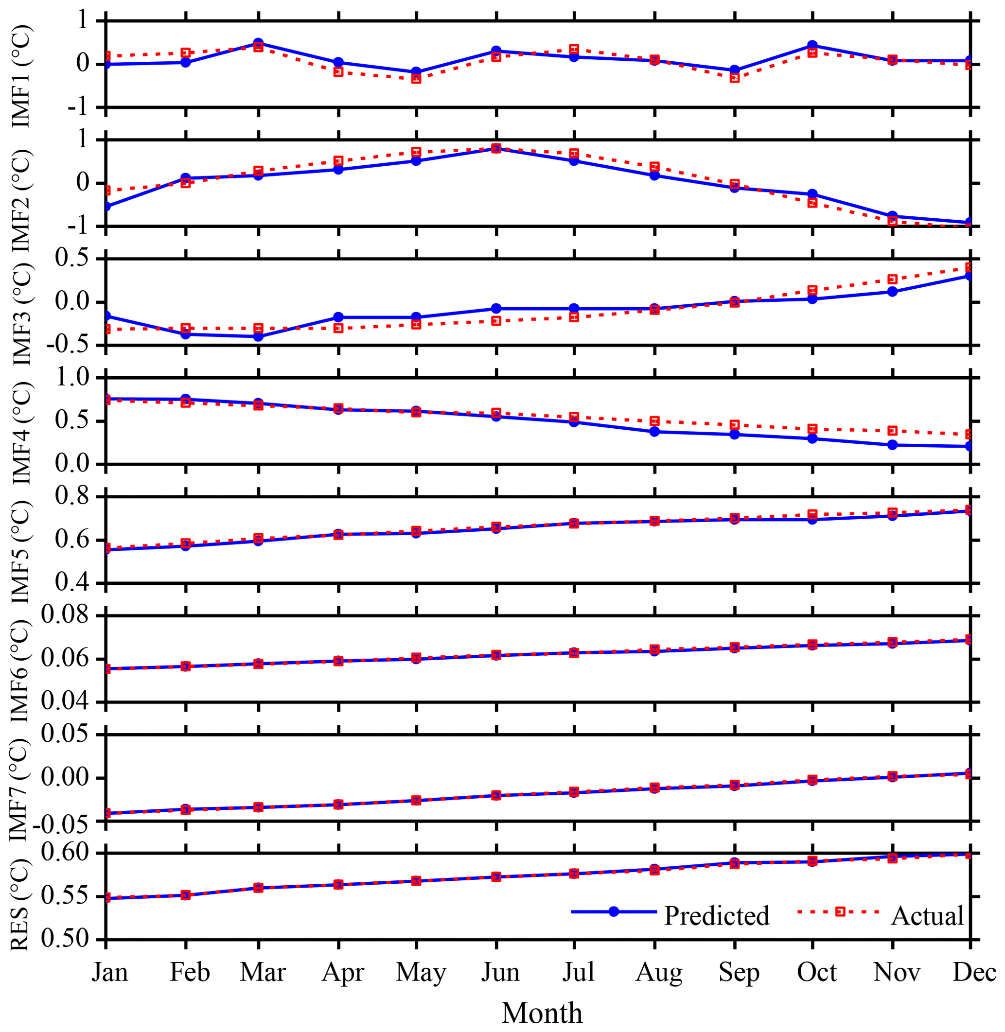
Figure 8 SSTA prediction results based on the hybrid EEMD-BPNN model of each individual component in 2017.

A three-layer BP neural network structure has been chosen and independently analyzed and predicted each month. For IMF4 and subsequent modes, the non-stationarity has been degraded relative to the first three modes; a BP neural network with 12 nodes at the input layer and output layer has been used to train and predict SSTA. The prediction results of each mode decomposition component based on the EEMD algorithm are shown in Fig. 8. The absolute errors of the predicted value and the actual value are shown in Table 1.

Root mean square error (RMSE) is used as a metric to assess the performance of the two different models:

$$\begin{array}{}\text{(2)}& {\displaystyle }{\displaystyle }\mathrm{RMSE}=\sqrt{{\displaystyle \frac{\mathrm{1}}{N}}\sum _{n=\mathrm{1}}^N{\left(x_n-y_n\right)}^{\mathrm{2}}},\end{array}$$

where x_n and y_n are the observed and the predicted values, respectively; N is the number of data used for the performance evaluation (N is 12 in this study). Results are shown in Table 1.

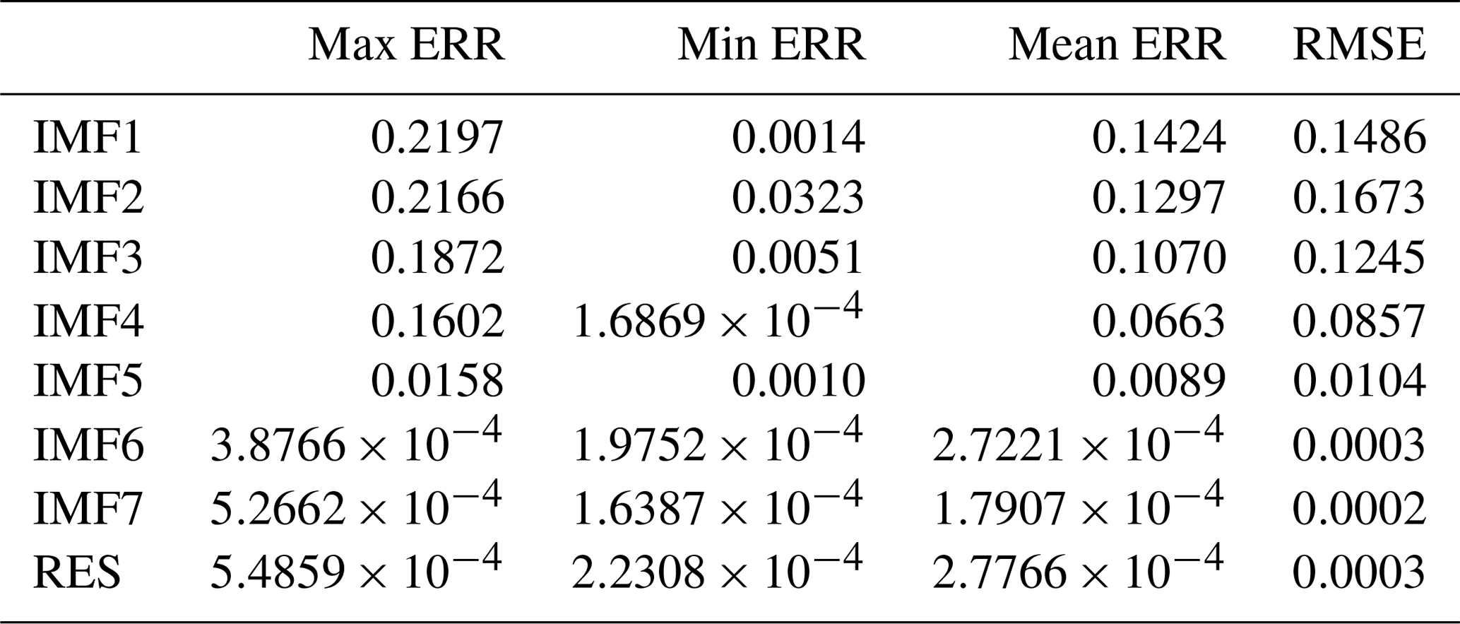
It can be seen from Fig. 8 and Table 1 that the maximum absolute error (max ERR) of the first decomposition component (IMF1) based on the hybrid EEMD-BPNN model is 0.2197 ^∘C in January. The minimum absolute error (min ERR) is 0.0014 ^∘C, which is in August. The prediction ability of the second mode decomposition component (IMF2) is roughly equivalent to IMF1, and the mean absolute error (mean ERR) of the first three intrinsic mode function components (IMF1, IMF2 and IMF3) is between 0.10 ^∘C and 0.15 ^∘C. The mean absolute errors of IMF4 and IMF5 are 0.0663 and 0.0089 ^∘C, respectively, and the prediction accuracy based on the hybrid EEMD-BPNN model is roughly equivalent to the decomposition accuracy of the EEMD algorithm. The prediction errors of the last two intrinsic mode function components and the RES are on the order of 10⁻⁴. It can be seen that, as the non-stationarity of the series data decreases, the error of the prediction results becomes smaller and smaller.

Table 1 The ERRs of the SSTA prediction results of each individual component based on the hybrid EEMD-BPNN model (unit: ^∘C).

According to the same method, the eight mode components decomposed by CEEMD algorithm have been analyzed and predicted. The prediction results and error analysis have been shown in Fig. 9 and Table 2. It can be seen from Fig. 9 and Table 2 that the maximum error of the first decomposition component (IMF1) based on the hybrid CEEMD-BPNN model is 0.1779 ^∘C in May. The minimum error is 0.0068 ^∘C, which is in June.

Figure 9 SSTA prediction results based on the hybrid CEEMD-BPNN model of each individual component in 2017.

Table 2 The ERRs of the SSTA prediction results of each individual component based on the hybrid CEEMD-BPNN model (unit: ^∘C).

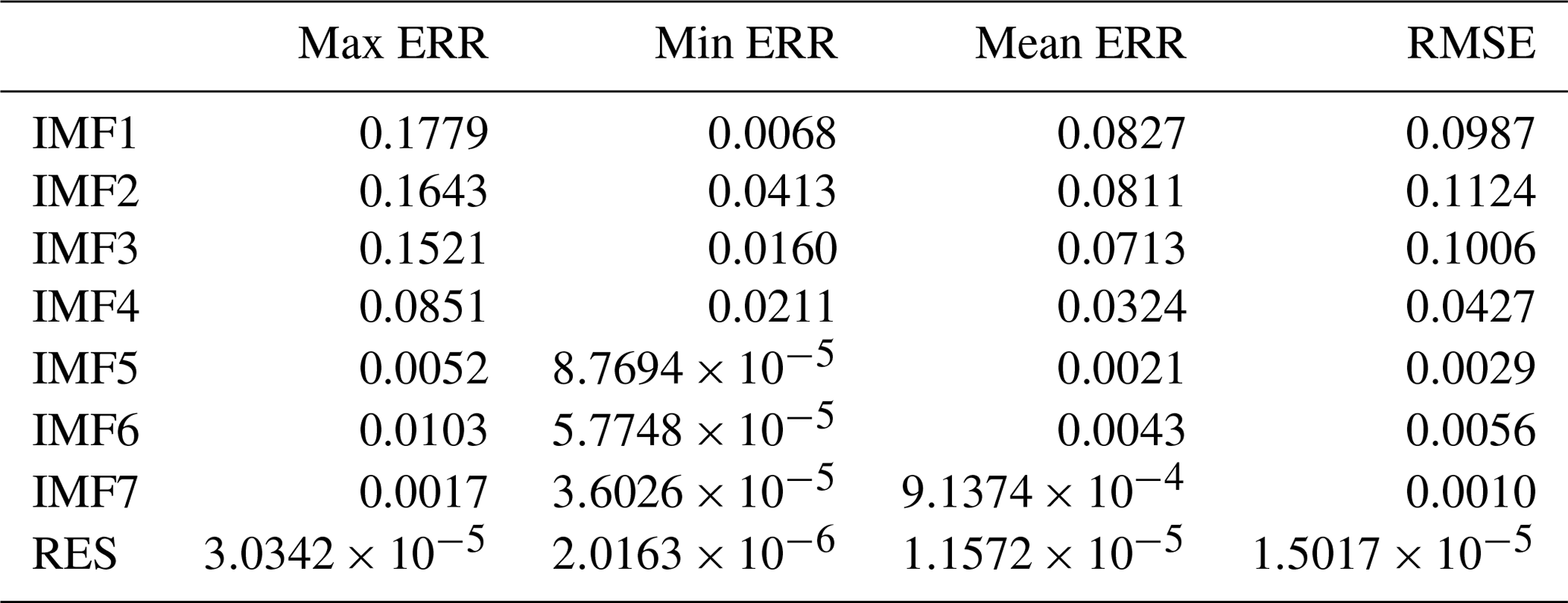
The prediction ability of the second mode decomposition component (IMF2) is roughly equivalent to IMF1. Except for the 4 months of May, September, October and November, the accuracies of prediction results of other months are satisfactory. The prediction results of the first three intrinsic mode function components (IMF1, IMF2 and IMF3) are basically the same as the actual data. In the prediction results of the fourth mode component (IMF4), except for a slight error in December, the prediction ability is better. The predicted results of the last three intrinsic mode function components (IMF5, IMF6, IMF7) and the RES are basically consistent with the observation results.

The prediction results of the monthly mean SSTA in 2017 are obtained by reconstructing the mode decomposition components (Fig. 10) and the ERR of prediction results have been shown in Table 3. It can be seen from the figure and table that the prediction results based on the EEMD-BPNN model have larger ERRs in January and August, exceeding 0.3 ^∘C, and the accuracies of prediction results in other months are satisfactory (the ERR is less than 0.3). The prediction accuracy based on the CEEMD-BPNN model is more satisfactory (ERR exceeds 0.1 ^∘C only in October), and the prediction ability based on the CEEMD-BPNN model is generally better than that of the EEMD-BPNN model.

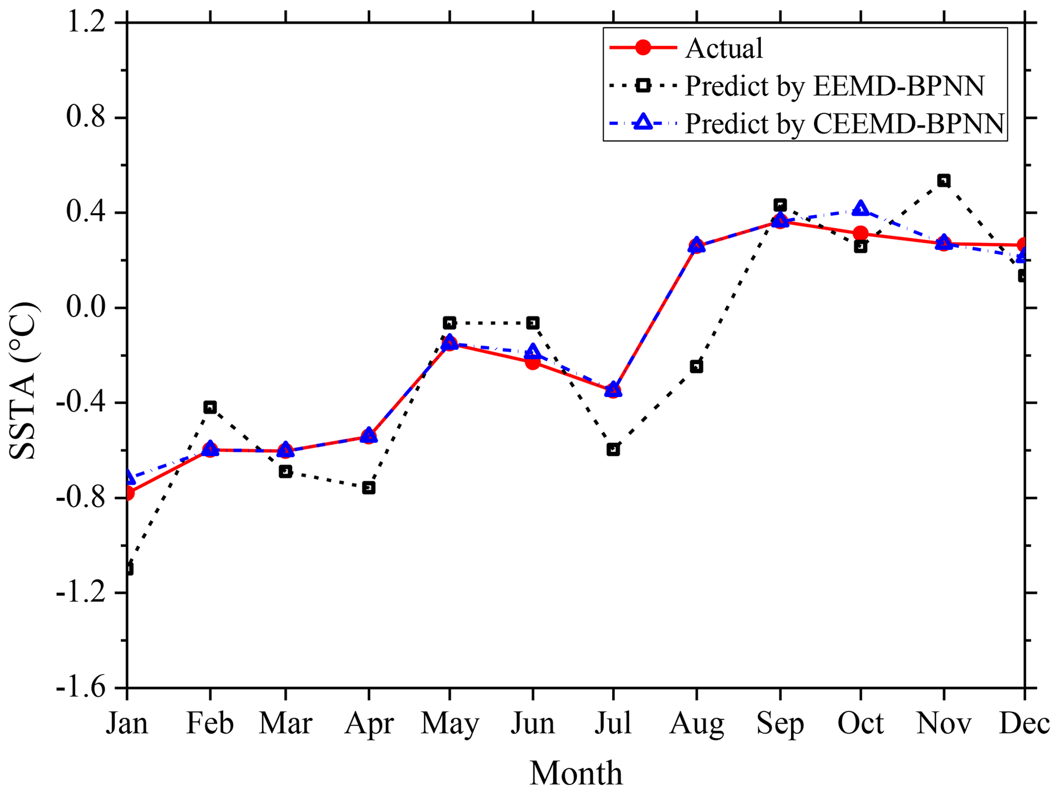
Figure 10 Monthly SSTA prediction results based on the hybrid improved EMD-BPNN models in 2017.

Table 3 The ERRs of the SSTA prediction results based on the two different hybrid improved EMD-BPNN models (unit: ^∘C).

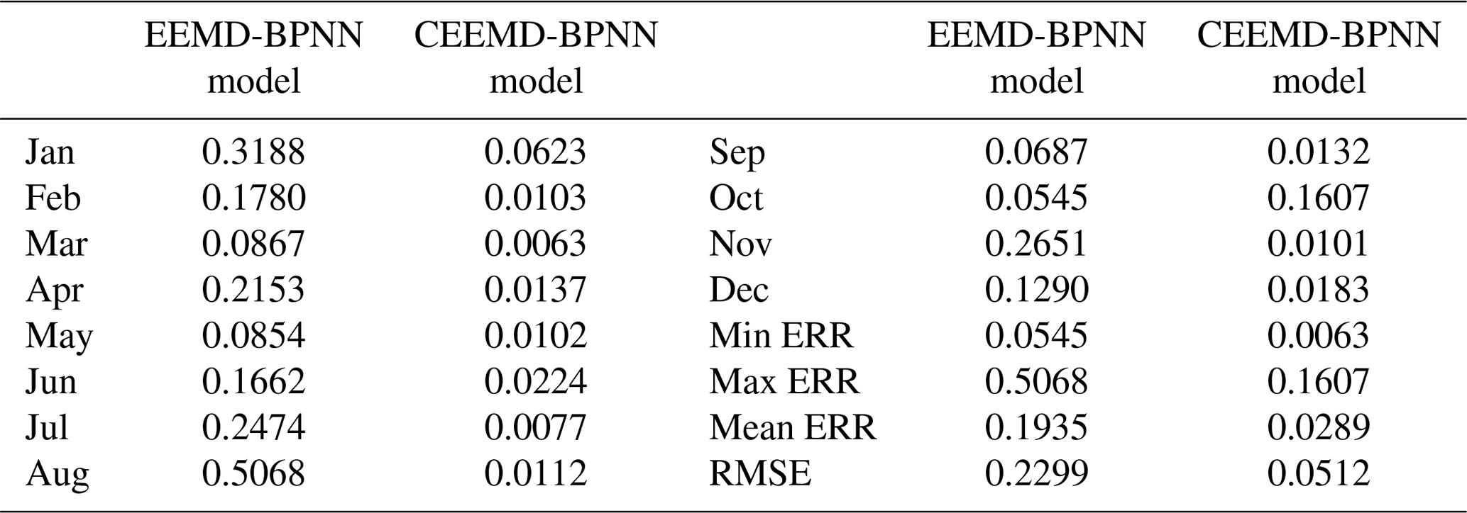
The correlation coefficient between the prediction values based on the CEEMD-BPNN model and observations is 0.97, indicating a significance level of 0.001. The result indicates that SSTA in 2017 was predicted accurately by the CEEMD-BPNN model. As can be seen from the above discussions, the ERR of decomposition components based on the EEMD and CEEMD algorithms will affect the accuracy of the final prediction results. Table 3 shows that prediction results of the hybrid CEEMD and BPNN model are much better than those of the EEMD-BPNN. This is because, after CEEMD, the original unsteady data are changed into certain components that have fixed frequency and periodicity. The CEEMD algorithm with less decomposition error has less error in the final prediction results, which proves that the CEEMD method has more advantages in data decomposition than the EEMD method. At the same time, we can find that the final prediction error of the two prediction models mainly comes from the first three mode decomposition components, and the error of the last five components has little effect on the accuracy of the final prediction results.

6 Conclusions

This paper presents an SST-predicting method based on the hybrid EMD algorithms and BP neural network method to process the SST data with nonlinearity and non-stationarity. Through EEMD and CEEMD algorithms, SSTA time-series data are decomposed into different IMFs and a RES. A BP neural network is applied to predict individual IMFs and the RES. Final results can be obtained by adding the predicting results of individual IMFs and RES.

In order to illustrate the effectiveness of the proposed approach, a case study was carried out. SSTA prediction results based on the hybrid EEMD-BPNN model and the hybrid CEEMD-BPNN model are discussed. In comparison, the proposed hybrid CEEMD-BPNN model is much better and its prediction results are more accurate.

From the absolute error of the prediction results of each IMF component and the absolute error of the predicted SSTA, the prediction error of SSTA mainly comes from the prediction of the first three mode decomposition components (IMF1, IMF2 and IMF3). SST prediction has been only preliminary, based on the two improved EMD algorithms and BP neural network in this paper. The results show that the hybrid CEEMD-BPNN model is more accurate in predicting SST. This work can provide a reference for predicting SST and El Niño in the future. In a follow-up study, how to improve the forecast duration is the focus.

It should be noted that some factors affecting the SST prediction results include the length and interval of the time series of the database, as well as different data sources because their values are also different. The SST time-series data in this study are based on NOAA OISST datasets from January 1982 to December 2016.