Atmospheric histories, growth rates and solubilities in seawater and other natural waters of the potential transient tracers HCFC-22, HCFC-141b, HCFC-142b, HFC-134a, HFC-125, HFC-23, PFC-14 and PFC-116

We present consistent annual mean atmospheric histories and growth rates for the mainly anthropogenic halogenated compounds HCFC-22, HCFC-141b, HCFC-142b, HFC-134a, HFC-125, HFC-23, PFC-14 and PFC-116, which are all potentially useful oceanic transient tracers (tracers of water transport within the ocean), for the Northern and Southern Hemisphere with the aim of providing input histories of these compounds for the equilibrium between the atmosphere and surface ocean. We use observations of these halogenated compounds made by the Advanced Global Atmospheric Gases Experiment (AGAGE), the Scripps Institution of Oceanography (SIO), the Commonwealth Scientific and Industrial Research Organization (CSIRO), the National Oceanic and Atmospheric Administration (NOAA) and the University of East Anglia (UEA). Prior to the direct observational record, we use archived air measurements, firn air measurements and published model calculations to estimate the atmospheric mole fraction histories. The results show that the atmospheric mole fractions for each species, except HCFC-141b and HCFC-142b, have been increasing since they were initially produced. Recently, the atmospheric growth rates have been decreasing for the HCFCs (HCFC-22, HCFC-141b and HCFC-142b), increasing for the HFCs (HFC-134a, HFC-125, HFC-23) and stable with little fluctuation for the PFCs (PFC-14 and PFC-116) investigated here. The atmospheric histories (source functions) and natural background mole fractions show that HCFC-22, HCFC-141b, HCFC-142b, HFC-134a, HFC-125 and HFC-23 have the potential to be oceanic transient tracers for the next few decades only because of the recently imposed bans on production and consumption. When the atmospheric histories of the compounds are not monotonically changing, the equilibrium atmospheric mole fraction (and ultimately the age associated with that mole fraction) calculated from their concentration in the ocean is not unique, reducing their potential as transient tracers. Moreover, HFCs have potential to be oceanic transient tracers for a longer period in the future than HCFCs as the growth rates of HFCs are increasing and those of HCFCs are decreasing in the background atmosphere. PFC-14 and PFC-116, however, have the potential to be tracers for longer periods into the future due to their extremely long lifetimes, steady atmospheric growth rates and no explicit ban on their emissions. In this work, we also derive solubility functions for HCFC-22, HCFC-141b, HCFC-142b, HFC-134a, HFC-125, HFC-23, PFC-14 and PFC-116 in water and seawater to facilitate their use as oceanic transient tracers. These functions are based on the Clark–Glew–Weiss (CGW) water solubility function fit and salting-out coefficients estimated by the poly-parameter linear free-energy relationships (pp-LFERs). Here we also provide three methods of seawater solubility estimation for more compounds. Even though our intention is for application in oceanic research, the work described in this paper is potentially useful for tracer studies in a wide range of natural waters, including freshwater and saline lakes, and, for the more stable compounds, groundwaters.

1 Introduction

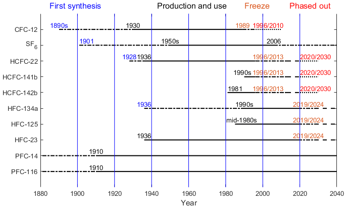
Oceanic and natural water transient tracers have time-varying sources and/or sinks. Chlorofluorocarbons (CFCs) were used traditionally as oceanographic transient tracers because of their continuously increasing atmospheric mole fractions until some years ago. They are powerful tools in oceanography for which they are used to, for instance, deduce transport times, estimate mixing rates between water masses, study formation rates of new water masses and determine the anthropogenic carbon (C_ant) content of seawater (Weiss et al., 1985; Waugh et al., 2006; Fine, 2011; Schneider et al., 2012; Stöven et al., 2016). The production and consumption of CFCs have been phased out as a consequence of the implementation of the Montreal Protocol (MP) on Substances that Deplete the Ozone Layer (first in developed nations by 1996, followed by developing nations by 2010) designed to halt the degradation of the Earth's protective ozone layer (Fig. 1). The atmospheric mole fractions of the major CFCs have been decreasing since the mid-1990s to early 2000s (Carpenter et al., 2014; Bullister, 2015), and although CFCs are valuable indices to quantify deep water transport, the use of CFCs as oceanographic transient tracers has become more difficult for recently ventilated water masses. During recent decades sulfur hexafluoride (SF₆) has been added to the suite of transient tracers measured in the ocean (Tanhua et al., 2004; Bullister et al., 2006). Its atmospheric mole fractions are still increasing and its atmospheric distribution is measured widely. However, SF₆ is also facing restrictions; for example, in Europe it has been banned for release as a tracer gas and in all applications except high-voltage switchgear since 1 January 2006 (Fig. 1). Since a combination of transient tracers is needed to constrain ventilation (Waugh et al., 2002; Stöven et al., 2015), it is necessary to explore other transient tracers with positive growth rates for the study of mixing and transport processes in the oceans and in other natural waters.

Figure 1 Comparison of production and use histories of CFC-12, SF₆, HCFCs, HFCs and PFCs.

1.1 Potential transient tracers

Generally, several requirements for a useful oceanic transient tracer can be defined: the tracer should have a well-established, transient source function (or well-defined decay function); have a low or well-known natural background; be conservative (not produced or destroyed) in the marine environment; and be measured relatively inexpensively, accurately and rapidly. Potential candidates as transient tracers that fulfill at least some of the requirements listed above include hydrochlorofluorocarbons (HCFCs) such as HCFC-22, HCFC-141b and HCFC-142b, hydrofluorocarbons (HFCs) such as HFC-134a, HFC-125 and HFC-23, and perfluorocarbons (PFCs) such as PFC-14 and PFC-116. As a first step in evaluating the usefulness of these compounds as oceanic transient tracers, we synthesize their atmospheric mole fraction histories and review their solubilities. An upcoming work will evaluate the in-field data on these compounds.

HCFC-22. Chlorodifluoromethane (CHClF₂) is the most abundant HCFC in the global atmosphere. It was first synthesized in 1928 and commercial use started in 1936 (Calm and Domanski, 2004). It has been used dispersedly in domestic and commercial refrigeration, as a spray-can propellant, and in extruded polystyrene foam industries (McCulloch et al., 2003; Jacobson, 2012) and nondispersedly as the feedstock in fluoropolymer production (Miller et al., 2010). HCFC-22 was first measured in the atmosphere in 1979 (Rasmussen et al., 1980); a pronounced increase in its abundance in the 1990s was found in both hemispheres as HCFC-22 became an interim replacement for CFC-12 since the late 1980s (Xiang et al., 2014). There are no known natural emission sources for HCFC-22 (Saikawa et al., 2012). A considerable amount of literature has been published on the atmospheric histories of HCFC-22. Montzka et al. (1993) presented the NOAA network measurements and historic mole fractions from a two-box model for HCFC-22 from 1980 to 1993, and these have since been updated and augmented with measurements from Antarctic firn air and box models to construct an atmospheric history and emissions for HCFC-22 from 1944 to 2014 (Montzka et al., 2010a, 2015). Sturrock et al. (2002) presented CSIRO HCFC-22 data from 1940 to 2000 based on an analysis of Antarctic firn air samples using the AGAGE instrumentation. In 2012, Saikawa et al. (2012) reported observations and archived air measurements from multiple networks, combined with the Model for OZone And Related chemical Tracers (MOZART), to present the atmospheric mole fractions for HCFC-22 from 1995 to 2009.

HCFC-141b. 1,1-Dichloro-1-fluoroethane (CH₃CCl₂F) has been widely used as a foam-blowing agent in rigid polyurethane foams for insulation purposes and in integral skin foams as a replacement for CFC-11. It was also employed as a solvent for lubricants, coatings and cleaning fluids for aircraft maintenance and electrical equipment as a replacement for CFC-113 (Derwent et al., 2007). The industrial production and use of HCFC-141b have greatly increased since the early 1990s, as have its global mole fractions and emissions (Oram et al., 1995; Sturrock et al., 2002; Montzka et al., 2015; Prinn et al., 2018a).

HCFC-142b. 1-Chloro-1,1-difluoroethane (CH₃CClF₂) has largely been emitted from extruded polystyrene board stock as a foam-blowing agent combined with small emissions from refrigeration applications as a replacement for CFC-12 (TEAP, 2003). Previous studies described measurements of HCFC-141b and HCFC-142b from the AGAGE network, UEA and CSIRO including measurements of the Cape Grim Air Archive (CGAA) and Antarctic firn air (Oram et al., 1995; Sturrock et al., 2002; Simmonds et al., 2017; Prinn et al., 2018a). NOAA flask and firn air measurements for both compounds have also been reported (Montzka et al., 1994, 2009, 2015).

HFC-134a. 1,1,1,2-Tetrafluoroethane (CH₂FCF₃) is the most abundant HFC in the Earth's atmosphere. It was first synthesized by Albert Henne in 1936 (Matsunaga, 2002). Extensive production and emission of HFC-134a began in the early 1990s. It was used as a preferred refrigerant in domestic, commercial and automotive air conditioning and refrigeration to replace CFC-12. It is also used to a lesser extent as a foam-blowing agent, cleaning solvent, fire suppressant and propellant in metered-dose inhalants and aerosols (Simmonds et al., 2015, 2017). Continuous and substantially increasing atmospheric levels of HFC-134a were found over the past 2 decades (Xiang et al., 2014). A number of researchers have reported the atmospheric history of HFC-134a. The observational record of HFC-134a started from near-zero levels in the background atmosphere (Oram et al., 1996). Montzka et al. (1996) reported initial measurements from the NOAA network for HFC-134a from the late 1980s to mid-1995, which have since been updated (Montzka et al., 2015). Simmonds et al. (1998) presented AGAGE observations for HFC-134a from 1994 to 1997, updated by O'Doherty et al. (2004) from 1998 to 2002, by Rigby et al. (2014) and by Prinn et al. (2018a) to recent times.

HFC-125. Pentafluoroethane (CHF₂CF₃) is currently the third most abundant HFC. It is used primarily in refrigerant blends for commercial refrigeration applications and has a minor use in fire-fighting equipment as a replacement for halons. Atmospheric mole fractions of HFC-125 are also rising consistently as one of the substitutes for CFCs (O'Doherty et al., 2009; Rigby et al., 2014; Prinn et al., 2018a). In 2009, O'Doherty et al. (2009) reported in situ and archived air measurements from Mace Head and Cape Grim, combined with the AGAGE 2-D 12-box model results for HFC-125 from 1977 to 2009. In 2015, Montzka et al. (2015) reported results of flask measurements of HFC-125 spanning from 2007 to 2013.

HFC-23. Fluoroform or trifluoromethane (CHF₃) is a by-product from the industrial production of HCFC-22. Historically it has been considered as waste and simply vented to the atmosphere, although process optimization and abatement can eliminate most or all emissions. HFC-23 was also used as a feedstock for halon-1301 (CBrF₃) production. Small amounts are reportedly used in semiconductor (plasma etching) fabrication, in very low-temperature refrigeration (dispersive) and in specialty fire-suppressant systems (dispersive) (McCulloch and Lindley, 2007). HFC-23 was first reported in the background atmosphere by Oram et al. (1998) in samples dating back to 1978. It continued to increase in the atmosphere (Miller et al., 2010; Rigby et al., 2014; Simmonds et al., 2018) despite the voluntary and regulatory efforts in developed nations and abatement measures in developing nations financially supported by the United Nations Framework Convention on Climate Change (UNFCC) Clean Development Mechanism (CDM). In the past 3 decades, a number of researchers have reported the atmospheric mole fractions of HFC-23. In 1998, Oram et al. (1998) reported measured and model-generated mole fractions of HFC-23 at Cape Grim from 1978 to 2005. Updated in situ AGAGE measurements and results from the AGAGE 2-D atmospheric 12-box chemical transport model for HFC-23 from 1978 to 2010 and from 1950 to 2016 have been presented by Miller et al. (2010) and Simmonds et al. (2018), respectively. A history derived from multiple firn air sample collections was also published in 2010 (Montzka et al., 2010a).

PFC-14. Tetrafluoromethane or carbon tetrafluoride (CF₄) is the most abundant perfluorocarbon (PFC) in the Earth's atmosphere and is one of the most long-lived tracer gases with an atmospheric lifetime of more than 50 000 years. The presence of carbon tetrafluoride in the atmosphere was first deduced by Gassmann (1974) from an analysis of contaminant levels of PFC-14 in high-purity krypton samples. The first atmospheric measurements of PFC-14 were made by Rasmussen et al. (1979). It has a background atmospheric mole fraction due to its natural source from the rocks and soils, especially tectonic activity (Deeds et al., 2015). The preindustrial level was 34.05±0.33 ppt for PFC-14 (Trudinger et al., 2016). The primary anthropogenic sources of PFC-14 are aluminum production, the semiconductor industry (Khalil et al., 2003; Mühle et al., 2010; Fraser et al., 2013) and perhaps the production of rare earth elements. Consequently, atmospheric mole fractions have approximately doubled since the early 20th century (Mühle et al., 2010; Trudinger et al., 2016; Prinn et al., 2018a).

PFC-116. Hexafluoroethane (C₂F₆) is another long-lived tracer gas with an atmospheric lifetime of at least 10 000 years. The tropospheric abundance of PFC-116 was first determined by Penkett et al. (1981). It has a small natural abundance (Mühle et al., 2010; Trudinger et al., 2016); the preindustrial level has been estimated to be 0.002 ppt (Trudinger et al., 2016). Like CF₄ it is also emitted as a by-product of aluminum production (Fraser et al., 2013) and during semiconductor manufacturing.

Table 1 Atmospheric lifetimes, ocean partial lifetimes, ozone depletion and global warming potentials of HCFC-22, HCFC-141b, HCFC-142b, HFC-134a, HFC-125, HFC-23, PFC-14 and PFC-116.

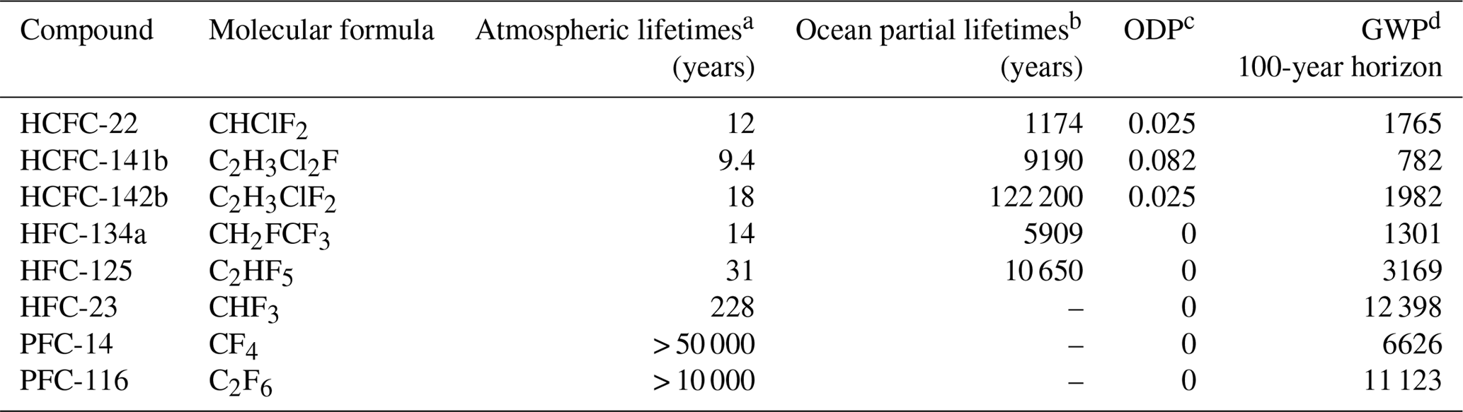
^a See SPARC (2013). ^b Partial atmospheric lifetimes with respect to oceanic uptake; see Yvon-Lewis and Butler (2002) and Carpenter et al. (2014). ^c ODP: ozone depletion potential; see Laube et al. (2013). ^d GWP: global warming potential; see Hodnebrog et al. (2013).

1.2 Production and ban histories

The major atmospheric degradation pathway of HCFCs and HFCs is through reaction with hydroxyl radicals (OH) in the troposphere (Montzka et al., 2010b). Combustion in thermal power stations has been pointed out as a tropospheric sink of PFCs (Cicerone, 1979; Ravishankara et al., 1993; Morris et al., 1995). The atmospheric lifetimes, ocean partial lifetimes, ozone depletion potentials (ODPs) and global warming potentials (GWPs) for HCFC-22, HCFC-141b, HCFC-142b, HFC-23, HFC-134a, HFC-125, PFC-14 and PFC-116 are listed in the Table 1. As shown Table 1, the atmospheric lifetimes of HCFCs and HFCs with respect to hydrolysis in seawater are very long (Yvon-Lewis and Butler, 2002; Carpenter et al., 2014), ranging from thousands to millions of years, indicating that HCFCs and HFCs are relatively stable in seawater. PFCs have atmospheric lifetimes on the order of thousands of years and very low solubilities in seawater. The production and use histories of CFC-12, SF₆, HCFCs, HFCs and PFCs are plotted in Fig. 1. HCFCs have been regulated with the aim of ceasing production and consumption by 2020 for non-Article 5 (developed) countries and 2030 for Article 5 (developing) countries (although this only covers dispersive applications) and phaseout beginning with a freeze in 1996 for developed nations and in 2013 for developing nations under the MP and its more recent amendments. Because of the high GWP of HFCs, 197 countries recently committed to cutting the production and consumption of HFCs by more than 80 % over the next 30 years under the Kigali Amendment of the MP, although not all of these countries have ratified this amendment. The reductions in HFC production and consumption are based on GWP-weighted quantities. Developed countries that have ratified the amendment have agreed to reduce HFC consumption beginning in 2019. Most developing countries will freeze consumption in 2024, some in 2028. This measure will most likely slow down HFC growth rates, eventually leading to a decline in their atmospheric mole fraction, similar to what is observed for CFCs.

In order to explore if these halogenated compounds can be used as transient ocean tracers, their atmospheric histories (source functions) and natural background should be established. Previous work has reconstructed annually averaged atmospheric mole fraction histories for some trace gases for use in tracer oceanographic applications. For example, Walker et al. (2000) reported annual mean atmospheric mole fractions for CFC-11, CFC-12, CFC-113 and CCl₄ for the period 1910–1998 and updated the data to 2008 on the website (http://bluemoon.ucsd.edu/pub/cfchist/, last access: 20 December 2018). On the basis of Walker's work, Bullister (2015) reported atmospheric histories for CFC-11, CFC-12, CFC-113, CCl₄, SF₆ and N₂O for the period 1765–2015. Previous work related to our target compounds has mainly focused on the atmospheric history over specific periods, often at a high temporal resolution. We have listed these works above. For our purposes, we are interested in a consistent record of the full atmospheric history at annual temporal resolution. As Trudinger et al. (2016) presented the consistent atmospheric histories of PFC-14 and PFC-116 from 1900 to 2014, we only study the growth rates for these two compounds and evaluate their utility as oceanic transient tracers.

In this study, drawing on previous literature and published data, we present atmospheric mole fractions (JFM means, annual means and JAS means) and growth rates for HCFC-22, HCFC-141b, HCFC-142b, HFC-134a, HFC-125, HFC-23, PFC-14 and PFC-116 for both the Northern (NH) and Southern Hemisphere (SH). The JFM means (the average of monthly means in January, February and March) and JAS means (the average of monthly means in July, August and September) are chosen to coincide with the coldest part of the year in the NH and SH, respectively, i.e., the time of (deep) water mass formation when ambient trace gases are carried from the surface to the interior ocean. The reconstructed atmospheric histories have been compiled from a combination of air measurements and model calculations. In order to provide a comprehensive and consistent view of halogenated compound atmospheric distribution and changes over time, ambient air measurements published by the Advanced Global Atmospheric Gases Experiment (AGAGE), the Scripps Institution of Oceanography (SIO), the Commonwealth Scientific and Industrial Research Organization (CSIRO), the National Oceanic and Atmospheric Administration (NOAA) and the University of East Anglia (UEA) are considered in this study. The calibration scale differences of these networks in the form of scale conversion factors are determined. SIO and CSIRO data are reported on AGAGE scales. NOAA and UEA data are converted to AGAGE scales by these conversion factors. For years prior to atmospheric observations, the reconstructed dry mole fractions for each species were provided by a combination of atmospheric models, firn air measurements and the analysis of archived air samples. The aim of this work is to synthesize existing data and model results into one consistent data product of atmospheric history with annual values useful for ocean tracer applications; it is not intended to replace more detailed atmospheric studies. All reported values in this study are dry air mole fractions. In a similar work, Meinshausen et al. (2017) provided consolidated datasets of historical atmospheric mole fractions of 43 greenhouse gases (GHGs). Compared with this earlier study, the differences and added value of this study are that we (1) incorporated UEA data not included in the Meinshausen et al. (2017) study, (2) report data on a common calibration scale (AGAGE) by converting NOAA and UEA data to AGAGE scales, (3) estimated annual means based on baseline data with local pollution events removed, (4) estimated the propagated uncertainties based on the original standard deviations of monthly means or data points, (5) used a different method for data fitting, and (6) presented the atmospheric histories for winter (JFM means in the NH and JAS means in the SH), which is especially useful for oceanic transient tracers studies.

In addition, we explore whether these compounds can be used as oceanic transient tracers by reporting on the solubility characteristics of each of the gases. We are not aware of any published estimates that directly provide solubility functions of all target compounds in seawater, and only very limited studies (with several data points) on the solubility of these compounds in seawater have been reported. Scharlin and Battino (1995) published four solubility data points in the temperature range 15–30 ^∘C and a salinity of 35.086 for PFC-14 in seawater. In the present analysis, the water and seawater solubility functions of HCFC-22, HCFC-141b, HCFC-142b, HFC-134a, HFC-125, HFC-23, PFC-14 and PFC-116 are derived by the combined method based on the combination of the Clark–Glew–Weiss (CGW) fit to estimate their water solubility function and the poly-parameter linear free-energy relationships (pp-LFERs) to estimate their salting-out coefficients. Three concluded methods (the (revised) method II only based on the pp-LFERs, the combined method and the experimental method) for seawater solubility estimation are also provided for more compounds. Although the atmospheric histories and solubility functions in water and seawater of the target compounds are intended for oceanic research, the work described in this paper is potentially useful for studying a range of natural waters, including freshwater, saline lakes and groundwaters.

2 Data and methods

2.1 Data from the AGAGE network

2.1.1 AGAGE in situ measurements and instrumentation

In situ atmospheric measurements have been made by the Advanced Global Atmospheric Gases Experiment (AGAGE) (Prinn et al., 2000; O'Doherty et al., 2004, 2009; Miller et al., 2010; Mühle et al., 2010; Prinn et al., 2018a, b). The data are available on the AGAGE website (http://agage.eas.gatech.edu/, last access: 20 December 2018) where historic and the newest atmospheric measurements are reported. AGAGE provides measurements of more than 40 compounds, whereas we focus only on HCFC-22, HCFC-141b, HCFC-142b, HFC-134a, HFC-125, HFC-23, PFC-14 and PFC-116 (Table S1 in the Supplement). There are more than 10 AGAGE and affiliated stations globally, mostly located at coastal or mountain sites. Here we exclude all AGAGE stations at tropical latitudes that are periodically subjected to air masses originating in the other hemisphere (Prinn et al., 1992, 2000; Walker et al., 2000). Observations at the AGAGE remote stations Mace Head, Ireland (MHD; 53^∘ N, 10^∘ W), and Trinidad Head, California (THD; 41^∘ N, 124^∘ W), were assumed to represent 30–90^∘ N atmospheric mole fractions, whereas observations at Cape Grim, Tasmania (CGO; 41^∘ S, 145^∘ E), represent 30–90^∘ S mole fractions. Small latitudinal gradients in the AGAGE Mace Head and Trinidad Head observations of different compounds are present but assumed to be of minor importance to this work. These stations, their locations and the date ranges of the samples used in this study are listed in Table S1. The “pollution-free” monthly mean atmospheric mole factions and standard deviations for all target compounds are used in this study.

All ambient air measurements were carried out using two similar measurement technologies over time based on the cryogenic pre-concentration with gas chromatography separation and mass spectrometry detection (GC-MS). The initial instrument used was the ADS (adsorption–desorption system) with GC-MS, but in the early to mid-2000s this was replaced by the Medusa GC-MS with a doubled sampling frequency, upgraded sample pre-concentration methodologies, extended compound selection and improved measurement precisions. For more information on the instrumentation and the working standards, see Simmonds et al. (1995), Miller et al. (2008), Arnold et al. (2012) and Prinn et al. (2018a). For the measurement precision, see Prinn et al. (2018a).

2.1.2 AGAGE measurements of CSIRO and SIO archived air

To extend the available mole fraction records back in time, NH and SH air archive samples collected by CSIRO and SIO were measured using AGAGE instrumentation for target compounds. Southern Hemisphere Cape Grim Air Archive (CGAA) samples, which are background or “baseline” air, were collected at the Baseline Air Pollution Station, Cape Grim, Tasmania, by CSIRO and the Bureau of Meteorology. The samples have been cryogenically collected into 34 L electropolished stainless-steel canisters (Langenfelds et al., 1996; Fraser et al., 2017) since 1978. The CGAA samples were analyzed on Medusa-9 in the CSIRO laboratory at Aspendale (Miller et al., 2010). Northern Hemisphere (NH) samples used for this paper were filled during background conditions mostly at Trinidad Head, but also at La Jolla, California, Cape Meares, Oregon (courtesy of the Oregon Graduate Center via CSIRO, Aspendale, and the Norwegian Institute for Air Research, Oslo, Norway), and Point Barrow, Alaska (courtesy of Robert Rhew, University of California, Berkeley), and analyzed at SIO, La Jolla, on laboratory-based Medusa GC-MS instruments (Medusa-1, Medusa-7) (O'Doherty et al., 2009). A stepwise tightening filtering algorithm was applied based on their deviations from a fit through all data from each semi-hemisphere (including pollution-free monthly mean in situ data) to remove outliers (Mühle et al., 2010; Vollmer et al., 2016).

HFC-134a air archive data obtained using AGAGE instrumentation at CSIRO and SIO are reported here for the first time (Table S1d). The archived air measurements for HFC-125 reported by O'Doherty et al. (2009) are used in this study (Table S1e) and have been updated to include more present data. The CGAA archived air measurements for HCFC-22 reported by Miller et al. (1998) are used here. CGAA Medusa-3 and Medusa-9 measurements for HFC-23 from AGAGE reported by Miller et al. (2010) are also reported here (Table S1f). CSIRO SH and SIO NH archived air samples have been analyzed on AGAGE GC-MS instrumentation at CSIRO, Aspendale and at SIO, La Jolla, for PFC-14 and PFC-116 (Mühle et al., 2010).

2.1.3 AGAGE measurements of CSIRO firn air

The firn layer is unconsolidated snow overlaying an ice sheet. Large volumes (hundreds of liters) of air trapped in firn can be extracted for subsequent analysis. From the measured firn depth profiles, atmospheric histories can be derived using firn diffusion models. Firn air histories typically cover the period from the present day (or drilling date) to up to 100 years ago.

The firn air samples for HCFC-141b and HCFC-142b were collected from six depths at Law Dome, Antarctic, in 1997–1998 at the DSSW20K site (Table S1b and c) (Sturrock et al., 2002). The firn air samples were measured on the AGAGE ADS–GC-MS instrument at Cape Grim. Antarctic firn air samples have also been used for the reconstruction of the atmospheric histories of PFC-14 and PFC-116 (Trudinger et al., 2016).

2.2 Data from the NOAA network

2.2.1 NOAA flask measurements

Flask air measurements of the compounds considered in this study have been made by the National Oceanic and Atmospheric Administration (NOAA) as early as 1992 (Montzka et al., 1994, 1996, 2009, 2015). The data are available on the NOAA website (ftp://ftp.cmdl.noaa.gov/hats/, last access: 20 December 2018) where the latest atmospheric measurements are reported. There are many NOAA and affiliated stations globally. In order to be consistent with the chosen AGAGE stations, NOAA observations at only Mace Head, Ireland (MHD; 42 m above sea level; m a.s.l.), for HCFC-22, HCFC-141b, HCFC-142b and HFC-134a as well as Trinidad Head, USA (THD; 120 m a.s.l.), for HCFC-22, HCFC-141b, HCFC-142b, HFC-134a and HFC-125 are used to represent atmospheric mole fractions from 30–90^∘ N. The observations at Cape Grim, Australia (CGO; 164 m a.s.l.), represent the 30–90^∘ S mole fractions. These stations, their locations and the sampling dates of the samples used in this study are listed in Table S1 and are essentially identical to the corresponding AGAGE stations.

Air samples are analyzed in the NOAA/ESRL/GMD Boulder laboratory by GC-MS techniques for HCFC-22, HCFC-141b, HCFC-142b, HFC-134a and HFC-125. More details are given by Montzka et al. (1993, 1994, 1996, 2015). The working standards and measurement precision are also reported in these studies.

2.2.2 NOAA measurements of archived and shipborne air samples

Archived air and shipborne air measurements from both hemispheres for HCFC-141b and HCFC-142b are given in Thompson et al. (2004). The archived air samples for HCFC-141b and HCFC-142b have been obtained at Niwot Ridge (NWR; 40^∘ N, 106^∘ W) since 1986. The cruise air samples were collected during the Soviet–American Gas and Aerosol Experiment (SAGA) II cruise in the Pacific Ocean in 1987 (37^∘ N–30^∘ S, 160–170^∘ W).

Archived air and shipborne air measurements for HFC-134a were presented by Montzka et al. (1996). Samples were collected at NWR. Samples were obtained shipboard during two cruises, one in the Pacific Ocean in 1987 (SAGA II above) and in 1994 (41^∘ N–47^∘ S, 127–76^∘ W) and another in the Atlantic Ocean in 1994 (46^∘ N–48^∘ S, 14–60^∘ W).

2.2.3 NOAA measurements of firn air

The first measurements of HCFC-141b and HFC-134a in firn air were made by Butler et al. (1999) and showed that there are no natural sources for these compounds.

2.3 Data from the UEA network

UEA archived air

University of East Anglia (UEA) measurements on Cape Grim Air Archive subsamples (since 1978) and flask samples collected at Cape Grim are updated following the original publications for HCFC-141b, HCFC-142b (Oram et al., 1995) and HFC-134a (Oram et al., 1996). The Cape Grim archived air contains trace gas records known to be representative of background air in the Southern Hemisphere. UEA has analyzed subsamples of the Cape Grim Air Archive, whereas the CGAA has been analyzed directly on AGAGE instrumentation at Cape Grim, CSIRO, Aspendale and at the SIO, La Jolla (Sect. 2.1.2).

The Cape Grim archived air, which is located at CSIRO, Aspendale, was subsampled for the UEA at Aspendale and the UEA flask air samples were collected directly at Cape Grim; both were analyzed by GC-MS at the UEA for HCFC-141b, HCFC-142b and HFC-134a (Oram et al., 1995, 1996) (Table S1b and c). The working standards and measurement uncertainties were also shown in the abovementioned studies.

2.4 Data from models

In order to estimate atmospheric mole fractions before direct atmospheric measurements commenced, the results from published models, a two-box model for HCFC-22 (Montzka et al., 2010a) and the AGAGE 2-D atmospheric 12-box chemical transport model for HFC-23 (Cunnold et al., 1983, 1994; Miller et al., 2010; Rigby et al., 2011), PFC-14 and PFC-116 (Trudinger et al., 2016), are also included in this study (Table S1g and h).

The two-box model for HCFC-22 from Montzka et al. (2010a) considers the atmosphere as two boxes – one box representing each hemisphere. Each hemisphere is assumed to be well mixed and a standing vertical gradient is assumed. Using the two-box model, Montzka et al. (2010a) derived the atmospheric mole fractions from 1944 to 2009 for HCFC-22 by assuming a constant 0.95 scaling of global emissions estimated by the Alternative Fluorocarbons Environmental Acceptability Study (AFEAS).

The AGAGE two-dimensional atmospheric 12-box chemical transport model, used here for HFC-23, PFC-14 and PFC-116 mole fractions, contains four lower tropospheric boxes, four upper tropospheric boxes and four stratospheric boxes, with boundaries at 30^∘ N, 0 and 30^∘ S in the horizontal and 500 and 200 hPa in the vertical (Cunnold et al., 1983, 1994; Rigby et al., 2011). It has previously used to estimate mole fractions and emissions of CFC-11, CFC-12 and various other trace gases. Miller et al. (2010) derived mole fractions for HFC-23 for the period 1978-2009 through an inversion technique using this 2-D 12-box model, but not back to zero atmospheric mole fraction. Trudinger et al. (2016) calculated the atmospheric mole fractions of PFC-14 and PFC-116 in each semi-hemisphere since 1900 by combining the data from ice core, firn, air archive and in situ measurements, thus extending the work of Mühle et al. (2010).

Table 2 Primary calibration scale conversion factors for HCFC-22, HCFC-141b, HCFC-142b, HFC-134a, HFC-125 and HFC-23 between AGAGE (UB and SIO) and NOAA^a.

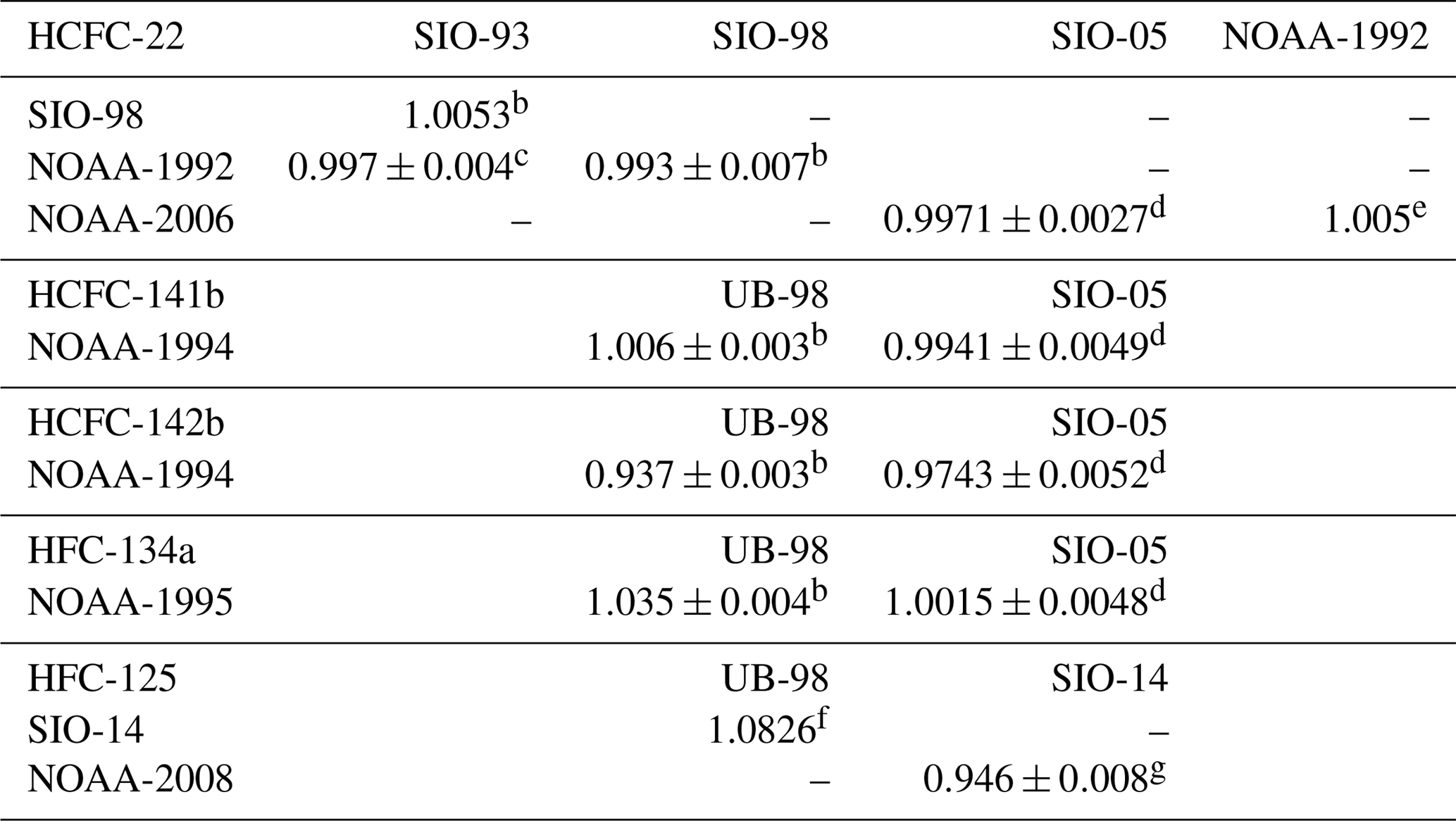
^a Example: for HCFC-22 measurement results reported on the SIO-98 scale, multiply 1.0053 to convert to the SIO-93 scale. AGAGE: Advanced Global Atmospheric Gases Experiment, UB: University of Bristol, SIO: Scripps Institution of Oceanography, NOAA: National Oceanic and Atmospheric Administration. ^b Prinn et al. (2000). ^c Miller et al. (1998). ^d Prinn et al. (2018a). ^e NOAA calibration scales for various trace gases (https://www.esrl.noaa.gov/gmd/ccl/scales.html, last access: 20 December 2018). ^f AGAGE calibration scale (http://agage.eas.gatech.edu/data_archive/agage/AGAGE_scale_2018_v1.pdf, last access: 20 December 2018). ^g Simmonds et al. (2017).

2.5 AGAGE, NOAA and UEA calibration scales

The latest AGAGE absolute calibration scales for various trace gases are displayed on the AGAGE website (https://agage.mit.edu/, last access: 20 December 2018 and http://agage.eas.gatech.edu/data, last access: 20 December 2018). AGAGE in situ measurements have been reported on the latest SIO absolute calibration scales for HCFC-22 (SIO-05), HCFC-141b (SIO-05), HCFC-142b (SIO-05), HFC-134a (SIO-05), HFC-125 (SIO-14), HFC-23 (SIO-07), PFC-14 (SIO-05) and PFC-116 (SIO-07), as have archived air measurements for HFC-134a and HFC-23. The archived air measurements for HFC-125 reported by O'Doherty et al. (2009) on the calibration scale UB-98 (UB: University of Bristol) were converted to the latest scale SIO-14 by the conversion factor SIO-14 ∕ UB-98 =1.0826 (see Table 2). The archived air measurements for HCFC-22 reported by Miller et al. (1998) on the calibration scale SIO-93 were converted to the latest scale SIO-05 by the combined conversion factors NOAA-1992 ∕ SIO-93 $=\mathrm{0.997}\pm \mathrm{0.004}$, NOAA-2006 ∕ NOAA-1992 =1.005 and NOAA-2006 ∕ SIO-05 $=\mathrm{0.9971}\pm \mathrm{0.0027}$ (see Table 2). The firn air measurements for HCFC-141b and HCFC-142b were reported on the calibration scale UB-98. Conversion factors NOAA-1994 ∕ UB-98 $=\mathrm{1.006}\pm \mathrm{0.003}$ and NOAA-1994 ∕ SIO-05 $=\mathrm{0.9941}\pm \mathrm{0.0049}$ are used to transfer data to the latest calibration scale SIO-05 for HCFC-141b (Prinn et al., 2000; Simmonds et al., 2017). For HCFC-142b, the data can be converted from scale UB-98 to the latest calibration scale SIO-05 by conversion factors NOAA-1994 ∕ UB-98 $=\mathrm{0.937}\pm \mathrm{0.003}$ and NOAA-1994 ∕ SIO-05 $=\mathrm{0.9743}\pm \mathrm{0.0052}$ (Prinn et al., 2000; Simmonds et al., 2017).

All NOAA absolute calibration scales for various trace gases are shown at https://www.esrl.noaa.gov/gmd/ccl/scales.html (last access: 20 December 2018). NOAA flask measurements were reported on the latest NOAA calibration scale for HCFC-22 (NOAA-2006), HCFC-141b (NOAA-1994), HCFC-142b (NOAA-1994), HFC-134a (NOAA-1995) and HFC-125 (NOAA-2008). NOAA archived air measurements for HCFC-141b and HCFC-142b were also reported on the latest scale. All data reported on NOAA scales are converted here to AGAGE calibration scale for both compounds. The conversion factors between AGAGE and NOAA are shown in Table 2 and were derived on the basis of Table 12 from Prinn et al. (2000), Table S4 from Simmonds et al. (2017) and Table 5 from Prinn et al. (2018a). The scale conversions between NOAA-1994 and SIO-98 for HCFC-22 in Prinn et al. (2000) were based on the comparison of gas mole fractions in air samples in 1994–1995, and the scale conversions between NOAA-1994 and UB-98 for HCFC-141b and HCFC-142b were based on the measurements against the NOAA standard and UB standard in 1997–1998. In the recent studies, the scale conversions between NOAA and AGAGE were based on the comparison of gas mole fractions in air samples in 1998–2017 for HCFC-22, HCFC-141b, HCFC-142b, and HFC-134 at CGO, SMO, THD and MSD (Prinn et al., 2018a). For HFC-125, the NOAA ∕ AGAGE ratio was based on the comparison in 2007–2015 at CGO, SMO and THD (Simmonds et al., 2017).

Archived air measurements from UEA are obtained on the NOAA-1994 scale for HCFC-141b and HCFC-142b and on the NOAA-1995 scale for HFC-134a. It is important to note that the original UEA calibration scale for HCFC-141b, HCFC-142b and HFC-134a (Oram et al., 1995, 1996) has been superseded by the NOAA scale. All UEA measurements obtained on the NOAA scale are converted to the AGAGE calibration scale by the conversion factors shown in Table 2.

2.6 Hemispheric annual mean and uncertainty estimation

We assembled data from in situ, flask, archived air and firn air measurements from the AGAGE, SIO, CSIRO, NOAA and UEA networks and/or laboratories as well as from AGAGE and NOAA model calculations (Table S1a–h). As the AGAGE baseline monthly means are nominally pollution-free data, the flask measurements from the NOAA network were processed by a statistical procedure to identify measurements that may have been influenced by regional pollution. Briefly, monthly means were calculated by averaging around four values for each month. Then the resultant standard deviations for each month were estimated by error propagation. For each month, values exceeding 3 standard deviations above the monthly mean were rejected as polluted. Afterwards, the monthly means for flask measurements were recalculated without pollution events, combined with UEA data and converted to AGAGE scales. The combined data from all networks and/or laboratories then formed the database used here.

The initial database containing replicate times has been converted into values without such replicates by using the number of measurement-weighted averages at each replicate time. That is to say, when measurements from different networks and sites are combined, hemispheric monthly averages were first calculated by weighted averages to give monthly means more weight as they are based on many individual measurements.

Hemispheric monthly means for each compound were estimated by a smoothing spline fit to the combined and sorted data. The inverses of the square of the standard deviations ((δy_i)⁻²) of each monthly mean or data points are used as the weights for the spline fit. Although there are no significant differences between the AGAGE and the NOAA monthly means in the same hemisphere, the hemispheric monthly means are closer to the AGAGE monthly means due to the much higher number of measurements in a given month from the AGAGE network (every 2 h, around 100–300 pollution-free samples per month for each site) compared to the NOAA network (weekly flask, around four samples per month for each site).

Hemispheric annual means were calculated by averaging the monthly means of the corresponding 12 months. The JFM means and JAS means are estimated by averaging monthly means of January, February and March and monthly means of July, August and September of the same year.

The smoothing spline fit method discussed above was based on previous studies (Reinsch, 1967; Craven and Wahba, 1978; Wahba, 1983, 1990; Hutchinson and De Hoog, 1985). The method is briefly described below. For more details, see Sect. S1 in the Supplement.

For a set of n data points taking values y_i at times t_i, the smoothing spline fit g(t) of the function g(t_i) is defined to be the minimizer of

$$\begin{array}{}\text{(1)}& p\sum _{i=\mathrm{1}}^n{\left[{\displaystyle \frac{g\left(t_i\right)-y_i}{\mathit{\delta }{y}_i}}\right]}^{\mathrm{2}}+\int g{}^{\prime \prime }(t{)}^{\mathrm{2}}\mathrm{d}t.\end{array}$$

Generally, the function is given an initial guess by sampling various values of the smoothing parameter p from 10⁻⁴, 10⁻³, …, 10¹⁰. The initial guess is the first local maximum. If it does not exist, the minimum location is used instead. The generalized cross-validation is used to estimate the smoothing parameter p. After estimating the optimal smoothing parameter, the estimated variance (VAR) and 95 % Bayesian confidence intervals (CI) are calculated. The weights (W) are assumed to be the inverse of the square of standard deviations ((δy_i)⁻²) associated with the observed variables. The spline is calculated as specified by Reinsch (1967).

The uncertainties of the final annual means are calculated based on the original uncertainties of the monthly means (e.g., for AGAGE in situ data, a standard deviation from 100–300 pollution-free measurements per month for each site) or the measurement precisions for individual data points. The uncertainties in the pollution-free AGAGE monthly means and the calculated NOAA monthly means include uncertainties in the measurements themselves (precision), scale propagation errors and sampling frequency errors. When the monthly means of the NOAA and UEA measurements were converted to AGAGE scales, scale conversion errors were also propagated. Following error propagation, the errors of the hemispheric monthly means were first calculated by the number of measurement-weighted root mean squares (RMSs) of the standard deviation of replicate values. The final uncertainties of hemispheric monthly means are calculated based on the misfit between the smoothing spline fit and the observed values. The uncertainties of hemispheric annual means were calculated as the square root of the squared errors from each of the 12 months.

2.7 Seawater solubility estimation method

Solubility has been reported in terms of the Henry's law solubility coefficient H (mol L⁻¹ atm⁻¹), the mole fraction solubility x (mol mol⁻¹), the Bunsen solubility coefficient β (L L⁻¹, in STP condition), the Ostwald solubility coefficient L (L L⁻¹), the weight solubility coefficient c_w (mol kg⁻¹ atm⁻¹) or the Künen solubility coefficient S (L g⁻¹). The definitions of solubility are shown in Young et al. (1982) and Gamsjäger et al. (2008, 2010). The relationship between different solubility terms is

$$\begin{array}{ll}{\displaystyle }H& {\displaystyle }={\displaystyle \frac{x}{(\mathrm{1}-x)\cdot p^{\ominus }\cdot V_{\mathrm{m}}}}={\displaystyle \frac{\mathit{\beta }}{R\cdot T^{\ominus }}}={\displaystyle \frac{L}{R\cdot T}}={\displaystyle \frac{c_w\cdot M_l}{V_{\mathrm{m}}}}\\ \text{(2)}& {\displaystyle }& {\displaystyle }={\displaystyle \frac{S\cdot M_g}{R\cdot T^{\ominus }\cdot V_{\mathrm{m}}}},\end{array}$$

where $T^{\ominus }=\mathrm{273.15}$ K and $p^{\ominus }=\mathrm{101.325}$ kPa =1 atm are the standard temperature and pressure (STP); V_m is the molar volume of the solvent, $V_{\mathrm{m}}=\mathrm{18.01528}\times {\mathrm{10}}^{-\mathrm{3}}$ L mol⁻¹ is the molar volume of water; R is the ideal gas constant, 8.314459848 L kPa K⁻¹ mol⁻¹ (or 0.08205733847 L atm K⁻¹ mol⁻¹); T is the temperature in Kelvin; and M_l is the molar mass of the solvent, which is 18.01528 g mol⁻¹ for water. Next, we present three methods to estimate the solubility of compounds in freshwater and seawater.

2.7.1 Method I: the CGW model

The following method to estimate the solubility of gases in seawater was reported in Deeds (2008) and is briefly described here. The Clark–Glew–Weiss (CGW) solubility equation can be used to calculate the solubility of gases in freshwater and seawater. It is derived from the integrated van 't Hoff equation and the Setschenow salinity dependence (Weiss, 1970, 1974) and expressed as a function of temperature and salinity.

$$\begin{array}{ll}{\displaystyle }\ln L& {\displaystyle }=a_{\mathrm{1}}+a_{\mathrm{2}}\cdot \left({\displaystyle \frac{\mathrm{100}}{T}}\right)+a_{\mathrm{3}}\cdot \ln \left({\displaystyle \frac{T}{\mathrm{100}}}\right)\\ \text{(3)}& {\displaystyle }& {\displaystyle }+S\left[b_{\mathrm{1}}+b_{\mathrm{2}}\cdot \left({\displaystyle \frac{T}{\mathrm{100}}}\right)+b_{\mathrm{3}}\cdot {\left({\displaystyle \frac{T}{\mathrm{100}}}\right)}^{\mathrm{2}}\right],\end{array}$$

where L is the Ostwald solubility coefficient in L L⁻¹ of a gas in seawater, T is the absolute temperature in Kelvin, S is the salinity in ‰ (or g kg⁻¹), and a_i and b_i are constants.

When S=0, this equation becomes the freshwater solubility equation for a gas:

$$\begin{array}{}\text{(4)}& \ln L_{\mathrm{0}}=a_{\mathrm{1}}+a_{\mathrm{2}}\cdot \left({\displaystyle \frac{\mathrm{100}}{T}}\right)+a_{\mathrm{3}}\cdot \ln \left({\displaystyle \frac{T}{\mathrm{100}}}\right),\end{array}$$

where L₀ is the Ostwald solubility in L L⁻¹ of a gas in freshwater.

We did not find complete studies on the solubility of our target gases in seawater based on experiments. Fortunately, the solubility of a gas in seawater can be determined from its freshwater solubility, which can be represented by a modified Setschenow equation (Masterton, 1975).

$$\begin{array}{}\text{(5)}& \ln \left(L_{\mathrm{0}}/L\right)=k_{\mathrm{s}}\cdot I_v\end{array}$$

Here L₀ is the freshwater solubility, L is the solubility in a mixed electrolyte solution, such as seawater, k_s is the salting-out coefficient and I_v is the ionic strength of the solution. k_s is an empirically derived, temperature-dependent constant. It can be estimated as a function of temperature using the freshwater and seawater solubility data by a least-square fit with a second-order polynomial (Masterton, 1975).

$$\begin{array}{ll}{\displaystyle }{k}_{\mathrm{s}}& {\displaystyle }=c_{\mathrm{1}}{t}^{\mathrm{2}}+c_{\mathrm{2}}t+c_{\mathrm{3}}=c_{\mathrm{1}}(T-\mathrm{273.15}{)}^{\mathrm{2}}\\ \text{(6)}& {\displaystyle }& {\displaystyle }+c_{\mathrm{2}}(T-\mathrm{273.15})+c_{\mathrm{3}},\end{array}$$

where t is the temperature in Celsius, T is the temperature in Kelvin and c_i represents the constants.

The ionic strength of seawater I_v (g L⁻¹) can be calculated from its salinity (S) (Deeds, 2008):

$$\begin{array}{}\text{(7)}& I_v={\displaystyle \frac{\mathrm{0.03600}}{\mathrm{1.80655}}}\times S\times \mathit{\rho }(T,S),\end{array}$$

where ρ(T,S) is the density of seawater in kg L⁻¹ estimated using the equation of state of seawater (Millero and Poisson, 1981). This equation is suitable for temperature (T) from 273.15 K (0 ^∘C) to 313.15 K (40 ^∘C) and salinities (S) from 0.5 to 43.

The seawater solubility of the target compounds based on method I can therefore be estimated by combining Eqs. (4), (5), (6) and (7).

$$\begin{array}{ll}{\displaystyle }\ln L& {\displaystyle }=\left[a_{\mathrm{1}}+a_{\mathrm{2}}\cdot \left({\displaystyle \frac{\mathrm{100}}{T}}\right)+a_{\mathrm{3}}\cdot \ln \left({\displaystyle \frac{T}{\mathrm{100}}}\right)\right]\\ {\displaystyle }& {\displaystyle }\cdot \exp [-(c_{\mathrm{1}}{\left(T-\mathrm{273.15}\right)}^{\mathrm{2}}+c_{\mathrm{2}}(T-\mathrm{273.15})+c_{\mathrm{3}})\\ \text{(8)}& {\displaystyle }& {\displaystyle }\times {\displaystyle \frac{\mathrm{0.03600}}{\mathrm{1.80655}}}\times S\times \mathit{\rho }(T,S)]\end{array}$$

2.7.2 Method II: the pp-LFER model

The solubility estimation of compounds is based on a cavity model: the poly-parameter linear free-energy relationships (pp-LFERs) in Abraham (1993). The pp-LFER model has been applied and validated for many types of partition coefficients (Abraham et al., 2004, 2012). In this model, the process of dissolution of a gaseous or liquid solute in a solvent involves setting up various exoergic solute–solvent interactions. Each of these interactions is presented in relevant solute parameters or descriptors. The selected Abraham model solute descriptors are the excess molar refraction (E) in cm³ mol${}^{-\mathrm{1}}/\mathrm{10}$, the solute dipolarity–polarizability (S), the overall solute hydrogen-bond acidity (A) and basicity (B), the McGowan's characteristic molar volume (V) in cm³ mol${}^{-\mathrm{1}}/\mathrm{100}$, and the gas–hexadecane partition coefficient (log L¹⁶) at 298.15 K.

$$\begin{array}{}\text{(9)}& {\displaystyle }& {\displaystyle }\log \mathrm{SP}=c+eE+sS+aA+bB+vV\text{(10)}& {\displaystyle }& {\displaystyle }\log \mathrm{SP}=c+eE+sS+aA+bB+l\log L^{\mathrm{16}}\end{array}$$

In these equations, the dependent variable logSP is some property of a series of solutes in a given system. Therefore, SP could be the partition coefficient, P, for a series of solutes in a given water–solvent system in Eq. (9) or L for a series of solutes in a given gas–solvent system in Eq. (10).

In this work, logSP refers to some solubility-related property of a series of gaseous solutes in water. SP is the gas–water partition coefficient K_w, which can be defined in terms of the equilibrium mole fractions of the solute through Eq. (11).

$$\begin{array}{}\text{(11)}& K_{\mathrm{w}}={\displaystyle \frac{\mathrm{Conc}.\mathrm{of}\mathrm{solute}\mathrm{in}\mathrm{water},\mathrm{in}\mathrm{mol}{\mathrm{dm}}^{-\mathrm{3}}}{\mathrm{Conc}.\mathrm{of}\mathrm{solute}\mathrm{in}\mathrm{the}\mathrm{gas}\mathrm{phase},\mathrm{in}\mathrm{mol}{\mathrm{dm}}^{-\mathrm{3}}}}\end{array}$$

The Ostwald solubility coefficient L₀ (in L L⁻¹) is usually expressed as the gas–water partition coefficients K_w, which can be estimated by Eq. (10). But L₀ can be determined by both Eqs. (9) and (10) because the “solvent” in the “water–solvent partition coefficient” could also be gas phase (Abraham et al., 1994, 2001, 2012). Based on the definition of gas–water partition coefficients in Eq. (11), the values calculated from Eq. (9), the water–gas partition coefficients, should be the reciprocal of the real solubility coefficients. But they are not. When Abraham dealt with this in his work (Abraham et al., 1994, 2001, 2012), he already treated the SP in Eq. (9) as the Ostwald solubility coefficients L₀. So L₀ can be determined by both Eqs. (12) and (13) by rewriting Eqs. (9) and (10).

$$\begin{array}{}\text{(12)}& {\displaystyle }& {\displaystyle }\log L_{\mathrm{0}}=c+eE+sS+aA+bB+vV\text{(13)}& {\displaystyle }& {\displaystyle }\log L_{\mathrm{0}}=c+eE+sS+aA+bB+l\log L^{\mathrm{16}}\end{array}$$

Inspired by Endo et al. (2012) and Goss et al. (2006), using the pp-LFER model to estimate the salting-out coefficients based on corrected V (V_c) (described afterwards), V_c, replaced V in Eq. (12) with the same coefficients and other descriptors. It was also used to calculate the Ostwald solubility coefficient in water, expressed as Eq. (14), for comparison.

$$\begin{array}{}\text{(14)}& \log L_{\mathrm{0}}=c+eE+sS+aA+bB+v{V}_{\mathrm{c}}\end{array}$$

L₀ values estimated by Eqs. (12), (13) and (14) based on V, log L¹⁶ and V_c were compared with the observed values. The estimated L₀ closest to the observed values will be chosen as the one to estimate the Ostwald solubility coefficients in water for the pp-LFER model method.

Table 3 Regression coefficients in equations for partition.

^a n is the number of data points. ^b r is the correlation coefficient. ^c SD is the standard deviation. ^d F is the F statistic.

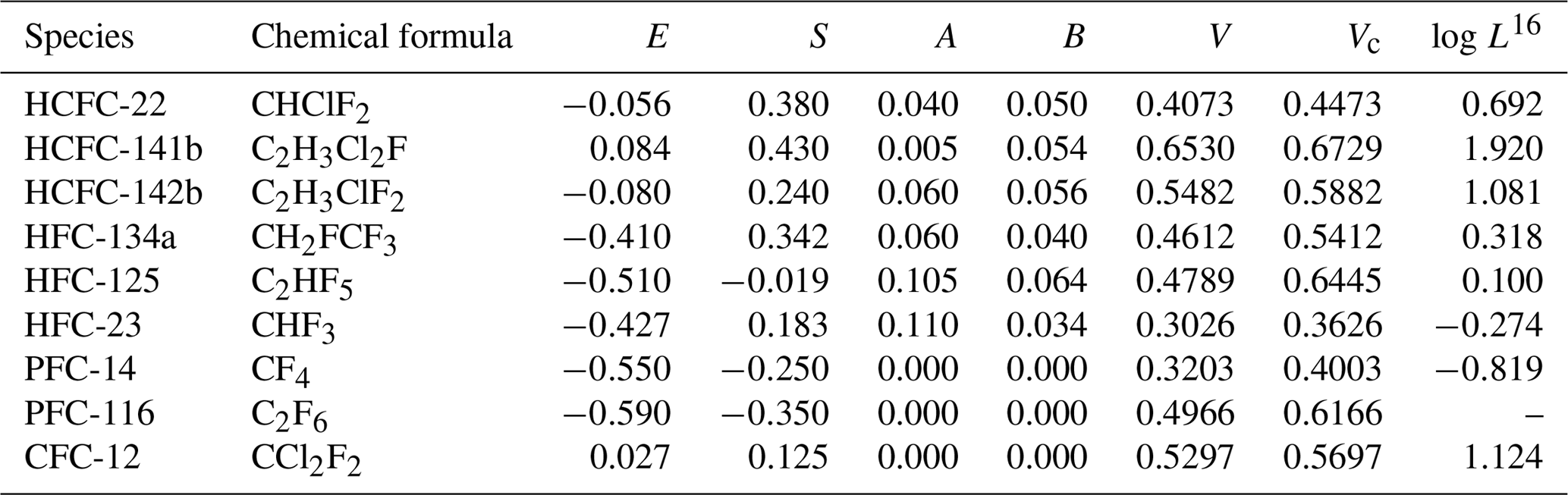
The set of coefficients, c, e, s, a, b, v and l characterize a solvent phase in terms of specific solute–solvent interactions. They are determined by multiple linear regression (MLR) analysis. The coefficients c, e, s, a, b, v and l for Eqs. (12), (13) and (14) at 298.15 and 310.15 K are shown in Table 3 (Abraham et al., 1994, 2001, 2012). The Abraham model solute descriptors E, S, A, B, V, V_c and logL¹⁶ are calculated based on different methods and shown in Table 4. E for target compounds except HCFC-22 and PFC-116 can be obtained from Abraham et al. (2001). For HCFC-22, the value of the E descriptor was calculated by Eq. (15) on the basis of the number of iodine, bromine, chlorine and fluorine atoms (nI, nBr, nCl and nF) in a halocarbon (Abraham et al., 2012) obtained from a regression analysis of 221 compounds. The methods of determining S, A, B descriptors are reported in previous studies (Abraham et al., 1989, 1991, 1993). The V descriptor, which is the measure of the size of a solute, is the molar volume of a solute calculated from McGowan's approach (McGowan and Mellors, 1986; Abraham and McGowan, 1987). The V_c descriptor is the corrected McGowan's characteristic molar volume with the characteristic atomic volume for a fluorine atom (Goss et al., 2006). L¹⁶ is the solute gas–hexadecane partition coefficient or the Oswald solubility coefficient in hexadecane at 298.15 K, which can be obtained from previous studies (Abraham et al., 1987, 2001, 2012).

Table 4 E, S, A, B, V, V_c and log L¹⁶ descriptors of HCFC-22, HCFC-141b, HCFC-142b, HFC-134a, HFC-125, HFC-23, PFC-14, PFC-116 and CFC-12 for the pp-LFER model.

$$\begin{array}{ll}{\displaystyle }& {\displaystyle }E=\mathrm{0.641}nI+\mathrm{0.328}nBr+\mathrm{0.140}nCl-\mathrm{0.0984}nF\\ \text{(15)}& {\displaystyle }& {\displaystyle }n=\mathrm{221},\mathrm{SD}=\mathrm{0.083}\end{array}$$

The solubility of a compound in salt solution can be determined from its solubility in water by Eq. (16). This equation is also the method for the quantitative description of the salting-out effect in neutral organic solutes, expressed in the following form using a modified Setschenow relationship (Sander, 1999; Schwarzenbach et al., 2003; Endo et al., 2012):

$$\begin{array}{}\text{(16)}& \log \left(L_{\mathrm{0}}/L\right)=K_{\mathrm{S}}\cdot \left[\mathrm{salt}\right],\end{array}$$

where L₀ is the Ostwald solubility coefficient in pure water (in L L⁻¹), L is the Ostwald solubility coefficient in the salt solution (in L L⁻¹), K_S is the molality-based Setschenow (or salting-out) coefficient (M⁻¹) for the salinity- and common-logarithm-based Setschenow equation and is independent of [salt], and [salt] is the molality of the salt in mol L⁻¹. The relationship between [salt] and salinity (S, g L⁻¹) in seawater is $\left[\mathrm{salt}\right]=S/M_{\mathrm{NaCl}}$. M_NaCl is the molar mass of sodium chloride (NaCl, 58.44 g mol⁻¹). So the salt mole fraction in seawater is approximately equivalent to 0.6 M NaCl (i.e., [NaCl] = ca. 0.6 M). It is best to define the salt solution based on molality. Adding dry salt to a solution does not change the molality of other solutes as the molality is the mass of the solvent rather than the solution (Sander, 1999).

The salting-out coefficient K_S should be estimated to calculate the solubility of a compound in a salt solution. K_S can be estimated by the poly-parameter linear free-energy relationships (pp-LFERs) since K_S is formally comparable with the common logarithm of the partition coefficient between the 1 M NaCl solution and freshwater (Abraham et al., 2012; Endo et al., 2012).

$$\begin{array}{}\text{(17)}& K_{\mathrm{S}}=c+eE+sS+aA+bB+v{V}_{\mathrm{c}}\end{array}$$

The coefficients c, e, s, a, b and v for Eq. (17) at 298.15±2 K are shown in Table 3 (Endo et al., 2012). E, S, A, B and V_c are the same as the ones described above. It is not easy to calculate the error in the descriptors as all the descriptors are calculated simultaneously (Abraham et al., 2001). E is calculated without error. V_c is the McGowan's characteristic molar volume without error. The general errors of S, A, B are thought to be 0.03 (Abraham et al., 1998, 2001). We assume that the error for each is 0.01 when S, A and B are all not zero and that the error is 0.03 for S and 0 for A and B when S is not zero but A and B are both zero. So the uncertainties of salting-out coefficients could be calculated by error propagation based on different functions. Using the above pp-LFER model, the Setschenow coefficient K_S can be estimated for numerous compounds with various functional groups (Endo et al., 2012).

The solubility of compounds in seawater based on the pp-LFER model can be estimated by combining one of the Eqs. (12), (13), (14) with Eqs. (16) and (17).

$$\begin{array}{}\text{(18)}& L=L_{\mathrm{0}}\cdot {\mathrm{10}}^{-K_{\mathrm{s}}\cdot \frac{S}{M_{\mathrm{NaCl}}}}\end{array}$$

In order to distinguish between Abraham's original method and the revised method based on his method in estimating Ostwald solubility coefficients in water, we name it “method II” when L₀ is calculated by Eqs. (12) or (13) and “revised method II” when L₀ is calculated by Eq. (14).

2.7.3 Combined method: combined CGW model and pp-LFER model

The main difference between the two methods described above to estimate the solubility of compounds in seawater is the different methods to estimate the water solubility and salting-out coefficients. Method I, reported in Deeds (2008), is mainly based on the Clark–Glew–Weiss (CGW) solubility model. The water solubility functions of compounds are constructed based on the CGW model and the salting-out coefficients are estimated as a function of temperature using the freshwater and seawater solubility data by the least-square fit with a second-order polynomial. In method I, more solubility measurements in water and seawater are needed and the chemical properties of compounds are considered. Method II is based on the poly-parameter linear free-energy relationships (pp-LFERs). The water solubility of compounds and salting-out coefficients are both estimated based on the pp-LFERs. Consideration of the physical properties of compounds is more important in method II. Both methods have shortages and advantages. For method I, there are frequently too few seawater solubility measurements for target compounds in order to construct the second-order polynomial between the salting-out coefficient and temperature. For method II, the water solubility functions for target compounds are only constructed at 298.15 and 310.15 K (Abraham et al., 2001, 2012).

The best approach is a combination of methods I and II to construct the solubility of compounds in water and seawater. The freshwater solubility functions of compounds can be constructed based on the Clark–Glew–Weiss (CGW) solubility model (method I) with the advantage of validity over a larger temperature range. The seawater solubility functions of compounds can be constructed on the basis of the pp-LFERs in estimating the salting-out coefficients (method II) with the advantage of working for more compounds. By combining Eqs. (4), (16) and (17), the solubility of compounds in seawater (L, Ostwald solubility coefficient in L L⁻¹) based on the combined method can be estimated by the following equation. This equation is used to estimate the seawater solubility of the target compounds in this paper.

$$\begin{array}{ll}{\displaystyle }L& {\displaystyle }={\mathrm{10}}^{-K_{\mathrm{S}}\cdot S/M_{\mathrm{NaCl}}}\cdot \exp \left[a_{\mathrm{1}}+a_{\mathrm{2}}\cdot \left({\displaystyle \frac{\mathrm{100}}{T}}\right)+a_{\mathrm{3}}\right.\\ \text{(19)}& {\displaystyle }& {\displaystyle }\left.\cdot \ln \left({\displaystyle \frac{T}{\mathrm{100}}}\right)\right]\end{array}$$

3 Results and discussion

3.1 Atmospheric histories and growth rates

During late winter, typically January, February and March in the Northern Hemisphere and July, August and September in the Southern Hemisphere, heat is lost from the surface seawater, which results in an increased density of the surface seawater. During this process, the mixed layer deepens and older water (usually with lower transient tracer mole fractions) is brought in contact with the atmosphere. The mixed layer gains density and tends to be transported towards the ocean interior through diffusive, advective and/or convective processes. This water then carries with it a signature of the atmospheric mole fraction, pending the saturation state of the water as it leaves the surface layer. For tracers with rapidly increasing atmospheric mole fractions and for deep mixed layers, under-saturation of the tracers has frequently been reported (e.g., Tanhua et al., 2008). Since we are interested in reporting the annual means for the compounds for their use as oceanic tracers of water masses, it is useful to know the atmospheric mole fractions of these compounds in late winter compared to annual means. JFM and JAS are nominally the coldest times in the Northern and Southern Hemisphere, respectively, and normally the main periods when water masses are formed. Therefore, we reconstructed JFM mean and JAS mean atmospheric mole fractions for all species in the Northern and the Southern Hemisphere. The annual mean atmospheric mole fractions of these compounds are mainly given to allow for comparison to the annual mean atmospheric mole fractions for CFC-11, CFC-12, CFC-113 and CCl₄ given in previous studies (Walker et al., 2000; Bullister, 2015).

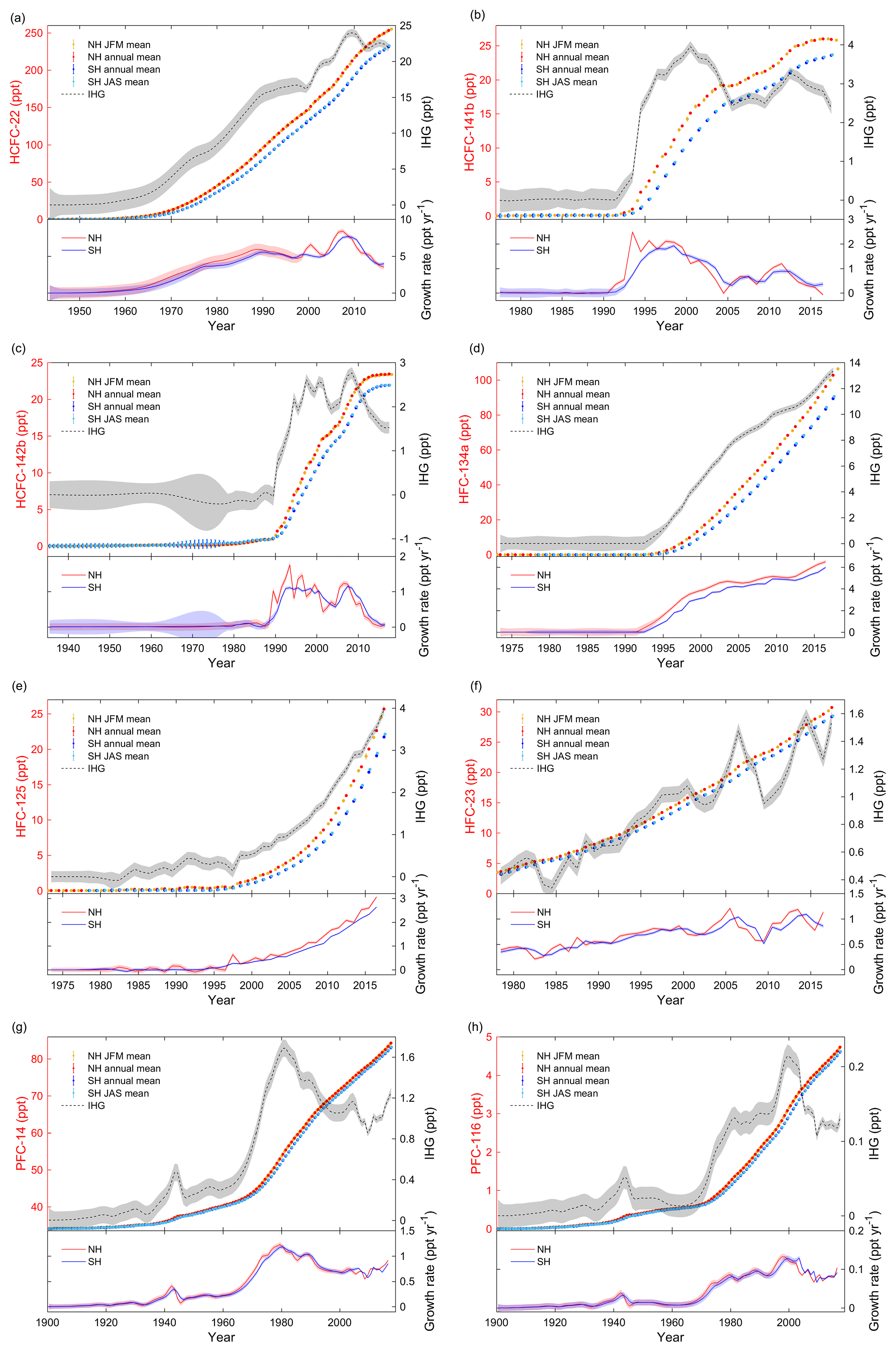
Figure 2 (a) HCFC-22: the top of the panel shows the JFM means (NH), annual means (NH and SH) and JAS means (SH) of atmospheric mole fractions and the interhemispheric gradients (IHG, in black, using the right axes). The lower section shows the annual growth rates in ppt yr⁻¹. Shadings in the figure reflect the uncertainties. (b) Similar to Fig. 2a, but for HCFC-141b. (c) Similar to Fig. 2a, but for HCFC-142b. (d) Similar to Fig. 2a, but for HFC-134a. (e) Similar to Fig. 2a, but for HFC-125. (f) Similar to Fig. 2a, but for HFC-23. (g) Similar to Fig. 2a, but for PFC-14. (h) Similar to Fig. 2a, but for PFC-116.

As described in Sect. 2, there are a number of datasets available for HCFC-22, HCFC-141b, HCFC-142b, HFC-134a, HFC-125, HFC-23, PFC-14 and PFC-116 (Table S1, Fig. S1a–h in the Supplement). Once consolidated into a single dataset via a common calibration scale, all data were fitted by a smoothing spline to determine the monthly means for each compound. The hemispheric annual mean, JFM mean (NH) and JAS mean (SH) atmospheric dry air mole fractions in parts per trillion (ppt) are then estimated and shown in Fig. S1a–h and the top of Fig. 2a–h. The associated uncertainties were estimated by error propagation and are shown at the top of Fig. 2a–h. The mole fractions and associated uncertainties are also given with JFM means (e.g., 2000.125), annual means (e.g., 2000.500) and JAS means (e.g., 2000.625) and shown in Table S2. Annual growth rates were calculated based on the annual means combined with their associated errors and are shown at the bottom of Fig. 2a–h. Interhemispheric gradients (IHGs) are estimated from the annual mean atmospheric mole fractions of a gas in the NH minus the annual mean in the SH in the same year (Fig. 2a–h). Errors of the IHG were estimated based on error propagation of the annual means in the NH and the SH in the same year (Fig. 2a–h).

3.1.1 HCFC-22

Annual mole fractions of HCFC-22 (Figs. 2a, S1a, Table S2) were 253.2±0.4 ppt (NH) and 231.2±0.3 ppt (SH) in 2017, which is a 23 % increase from 2009 (Montzka et al., 2010a). The interhemispheric gradient (IHG) initially increased but has been diminishing since 2010 because of a decline in emissions (growth rates). Growth rates for HCFC-22 rose steadily until 1990, followed by a slight decrease, which coincides with the large production and consumption reported between the 1950s and 1990s (Fig. 1) and a freeze of production magnitudes in developed countries in 1996. A rapid increase occurred between 2005 and 2008. Corresponding step changes were also seen in 2005 in both observations (upper panel in Fig. 2a) and emissions (Xiang et al., 2014) in response to the United Nations Environment Programme (UNEP) production changes (UNEP, 2018). The growth rate peaked in 2007 (NH) at 8.4 ppt yr⁻¹ and in 2008 (SH) at 7.6 ppt yr⁻¹ before a sharp 91 % decline to 2016 at an annual average rate of 0.8 ppt yr⁻² (NH) and 0.7 ppt yr⁻² (SH). This suggests that global emissions are not growing as rapidly as before 2008, as reported by Montzka et al. (2015) and Graziosi et al. (2015), consistent with the phaseout in the dispersive application of HCFCs since 2007 (Graziosi et al., 2015).

3.1.2 HCFC-141b

HCFC-141b (Figs. 2b, S1b, Table S2) annual mole fractions increased from 1990, and a slowdown occurred in the second half of the 2000s, corresponding to a sharp drop in production and consumption in 2005 (Montzka et al., 2015). HCFC-141b annual mole fractions have increased to a maximum of 26.0±0.1 ppt (NH) in 2016 and 23.6±0.1 ppt (SH) in 2017, representing 36 % (NH) and 41 % (SH) increases from 2005 and 7 % (NH) and 12 % (SH) increases from 2012. This also suggests that the annual mole fractions in the NH began to decrease. Rapid growth rates were seen before 1993 (NH) and 1995 (SH), coinciding with intensified industrial production and consumption of HCFCs in the 1990s. This is followed by a comparatively stable plateau period, 1994–1999 (NH) and 1995–1999 (SH), consistent with UNEP production (Montzka et al., 2015) and consumption changes (UNEP, 2018). Subsequently, the growth rate declined until around 2005. Since 2005, production has increased substantially in developing countries, so growth rates recovered to higher values in 2006–2007. Growth rates in 2012 appear to represent a 109 % (NH) and 59 % (SH) decline to 2016 of −0.07 ppt yr⁻¹ (NH) and 0.36 ppt yr⁻¹ (SH). The growth rates in 2016 are very close to the growth rates seen in the 1980s. This decline coincides with the global production and consumption of HCFCs being capped in 2013 in developing countries (Montzka et al., 2015).

3.1.3 HCFC-142b

Annual mean mole fractions for HCFC-142b (Figs. 2c, S1c, Table S2) show a slow initial increase until 1989 followed by a sharp increase in the 1990s, the same slowdown in the mid-2000s as seen with HCFC-141b, and finally a plateau in recent years. Annual mole fractions reached a maximum of 23.4±0.1 ppt (NH) and 21.9±0.1 ppt (SH) in 2017 at the end of the time series, representing a 39 % (NH) and 48 % (SH) increase since 2005. Annual mole fractions in the NH show a declining trend. The IHG and growth rates exhibit two peaks, one in the 1990s and another in 2007–2008, followed by a substantial drop. There are minima in growth rates around 2005 for all three HCFCs. The peak–valley–peak distribution patterns of HCFCs are consistent with the UNEP consumption changes (UNEP, 2018). For HCFC-142b, this is followed by a dramatic 99 % (NH) and 94 % (SH) decline to 2015 from 2007–2008 at an annual average rate of 0.14 ppt yr⁻² for both hemispheres. This decline in both atmospheric mole fractions and emissions follows reduced production and consumption in developed countries and a leveling-off of production and consumption in developing countries (Carpenter et al., 2014). The current growth rates for HCFC-142b are similar to those seen in the 1980s before the rapid increase in emissions.

3.1.4 HFC-134a

Annual mean mole fractions of HFC-134a (Figs. 2d, S1d, Table S2) have increased continuously since the 1990s. The monotonical increase is reflected in emissions (Xiang et al., 2014; Montzka et al., 2015; Simmonds et al., 2017). HFC-134a annual mole fractions reached a maximum of 102.7±0.2 ppt (NH) and 89.4±0.2 ppt (SH) by the end of the current time series, representing 163 % (NH) and 191 % (SH) increases since 2005 and 40 % (NH) and 42 % (SH) increases since 2012. IHG and growth rates started to increase around 1992, then rapidly increased in 1995–2004, followed by a stabilization of growth rate in 2009–2012 and then an increase since 2012. The maximum growth rates are shown at the end of the time series of 6.5 ppt yr⁻¹ (NH) and 6.0 ppt yr⁻¹ (SH), representing a 3.7–3.8 % per year increase from 2005 and a 6.3–6.5 % per year increase from 2012.

3.1.5 HFC-125

Annual mean mole fractions, IHG and growth rates of HFC-125 (Figs. 2e, S1e, Table S2) increased throughout the atmospheric history record, which reflects a continuing increase in emissions (O'Doherty et al., 2009; Montzka et al., 2015; Simmonds et al., 2017). Annual mole fractions reached a maximum of 25.7±0.1 ppt (NH) and 21.7±0.05 ppt (SH) at the end of the time series, representing 199 % (NH) and 216 % (SH) increases since 2009 (O'Doherty et al., 2009). The growth rate reached a peak of 3.1 ppt yr⁻¹ (NH) and 2.6 ppt yr⁻¹ (SH) by the end of the time series, representing 117 % (NH) and 138 % (SH) increases from 2009. The increase in the growth rate of HFC-125 is more than 3 times the growth rate increase for HFC-134a.

3.1.6 HFC-23

Annual mean mole fractions of HFC-23 (Figs. 2f, S1f, Table S2) have increased since 1978. HFC-23 atmospheric mole fractions peaked at 30.7±0.05 ppt (NH) and 29.2±0.06 ppt (SH) by the end of the time series (in 2017), representing a 4–4.1 % per year increase since 2009 (Miller et al., 2010). IHG and growth rates exhibit an increasing trend with large fluctuations over the time series, with local maxima in the growth rate in 2006 and 2013 and a minimum in 2009, which reflect changes in emissions (Carpenter et al., 2014; Simmonds et al., 2018). The slowing in growth rate was in response to emission reductions in developed countries that began in the late 1990s, combined with the UNFCCC CDM destruction program for developing countries that started around 2007 (Miller and Kuijpers, 2011; Carpenter et al., 2014). The higher values in growth rates could be attributed to the increase in production of HCFC-22 with no subsequent incineration of HFC-23 (Miller and Kuijpers, 2011; Carpenter et al., 2014). The current annual growth rates are 1.1 ppt yr⁻¹ (NH) and 0.86 ppt yr⁻¹ (SH), representing 100 % (NH) and 68 % (SH) increases since 2009. The increase in the growth rates for HFC-23 is between the ones for HFC-134a and for HFC-125.

3.1.7 PFC-14 (CF₄)

Trudinger et al. (2016) used a firn diffusion model to determine the atmospheric abundance of PFC-14 (Figs. 2g, S1g, Table S2) since 1900 from ice core, firn air, archived air and in situ measurements. Here we updated and extended the time series assembled by Trudinger et al. (2016). PFC-14 has a natural background of 34.05±0.33 ppt (Trudinger et al., 2016). Annual mean mole fractions and growth rates began to increase around 1900, with a local maximum in growth rate around 1943. The maximum reflects changing emissions from increasing aluminium production during World War II (Barber and Tabereaux, 2014; Trudinger et al., 2016), for example for the construction of aircraft. Mole fractions of PFC-14 began to increase rapidly in the 1970s. Since then it has continued to grow, reaching a maximum of 84.30±0.04 ppt (NH) and 83.05±0.03 ppt (SH) at the end of the time series (in 2017), representing 8 % (NH) and 7 % (SH) increases from 2009. The growth rates began to increase from the 1950s and peaked in 1980 before declining. The decline is attributed to a concerted effort by the aluminium and semiconductor industries to reduce their emissions (Trudinger et al., 2016). The growth rate minimum in 2009 could be related to the global financial crisis (Trudinger et al., 2016). PFC-14 growth rates have increased again during the last 5 years probably due to increased aluminium production and perhaps rare earth element production in developing countries (Vogel and Friedrich, 2018). The current growth rates are 0.91 ppt yr⁻¹ (NH) and 0.85 ppt yr⁻¹ (SH), representing 48 % (NH) and 49 % (SH) increases from 2009.

3.1.8 PFC-116

We updated and extended the time series previously shown in Trudinger et al. (2016). PFC-116 (Figs. 2h, S1h, Table S2) has a preindustrial background of 0.002 ppt (Trudinger et al., 2016). PFC-116 shows a similar atmospheric trend to PFC-14. Annual mean mole fractions have increased since ∼1900, with a step-up around 1943 (discussed above; PFC-116 is coproduced with PFC-14 during aluminium production), and increased significantly in the 1970s, reaching 4.73±0.007 ppt (NH) and 4.06±0.007 ppt (SH) by the end of the record, representing 16 % increases from 2009. PFC-116 growth rates began to increase slowly, followed by maxima around 1943 (discussed above for PFC-14). Then they declined and stayed relatively stable until 1965 when they started to climb to a maximum at the end of the 1990s. Subsequently, they declined and stayed relatively stable at 0.104 ppt yr⁻¹ (NH) and 0.09 (SH) ppt yr⁻¹.

Global annual mean mole fractions of HCFCs, HFCs and PFCs, except HCFC-141b and HCFC-142b, have increased continuously in the background atmosphere throughout the whole atmospheric history record (Fig. 2a–h). Recent growth rates are decreasing for HCFCs, increasing for HFCs and stable for PFCs. From Fig. 2a–h, it is clear that the mole fractions for target compounds in the NH are always larger than those in the SH but follow similar trends; the growth rates in both hemispheres are also similar (lagged in the SH) and the trends in IHG and in emissions and growth rates are very similar. This behavior is because the majority of the emissions (typically > 95 %) occur in the NH extratropics (O'Doherty et al., 2009; Saikawa et al., 2012; Carpenter et al., 2014; UNEP, 2018) and the interhemispheric mixing time is around 1 or 2 years. Thus, the larger the increase in emissions in the NH, the higher the resultant IHG. If all emissions stop, long-lived compounds would expect to reach near-identical mole fractions in both hemispheres.

3.2 Growth patterns

The atmospheric history trends of target compounds generally follow expected patterns based on the history of their known industrial applications and production bans. We can make out three distinct behavioral patterns with which we could predict the trend of annual mean mole fractions of these compounds. In pattern I, the annual mean mole fractions show sigmoidal (S-shaped) growth and the annual growth rates exhibit the shape of Gaussian distribution over the whole time period, such as HCFC-141b and HCFC-142b. This means that the annual mole fractions of these compounds are going to decrease or are decreasing. In pattern II, the annual mean mole fractions show initial exponential growth followed by a period of linear increase, while the growth rates show a sigmoidal pattern but a slight increase recently, such as HFC-134a and HFC-23 (combined with the modeled mole fraction output of HFC-23 from 1950 to 2016 shown in Fig. 1 in Simmonds et al., 2018). This means that the mole fractions of these compounds are going to continuously increase with relatively slower growth rates in the near future. Afterward, they will likely experience a plateau phase, followed by a decline following the restrictions imposed by the 2016 Kigali Amendment to the Montreal Protocol. Since the atmospheric lifetime of HFC-23 is much longer than that of HFC-134a, time profiles and IHG change are expected to be a little different between HFC-134a and HFC-23. In pattern III, the annual mean mole fractions and growth rates both show exponential (J-shaped) growth, such as HFC-125. So the atmospheric history and growth rates of HFC-125 are going to increase for a longer period of time than HFC-134a and HFC-23, and then will likely follow a similar path to the compounds in pattern II as they are subjected to the same regulations.

The annual mean mole fractions of the remaining halogenated compounds, HCFC-22, PFC-14 and PFC-116, have also increased throughout the time series and continue to increase today. The growth rates of these compounds initially increased and experienced a peak before declining. The growth trend for HCFC-22 is more likely to experience a plateau and then a decrease, following the trends of HCFC-141b and HCFC-142b as they are subjected to the same regulations. Different from all other target compounds, the annual mean growth rates of PFC-14 and PFC-116 have stabilized after a short decline without specific restrictions on emissions. This could be attributed to the changing sources of both PFC-14 and PFC-116. PFC emissions from the aluminium industry dominated for a long time but have likely been declining for the past decade or so, while emissions by the electronics industry (Kim et al., 2014) and probably the rare earth elements industry became more important. The very long lifetimes of PFCs in the atmosphere makes a decrease in the atmospheric mole fraction unlikely in the foreseeable future.

Considering the combined growth patterns and the production and consumption histories for these gases (Fig. 1), the sequence of atmospheric change in HCFCs and HFCs coincides with the replacement sequence of CFCs. In the 1980s, CFCs were found to be a threat to the ozone layer (Molina and Rowland, 1974; Rowland and Molina, 1975). To facilitate the phaseout of the more potent ozone-depleting CFCs, HCFC production and consumption increased rapidly in developed countries in the 1990s and in developing countries in the mid-2000s as industrial and domestic usage of CFCs was curtailed. Thus, atmospheric growth rates of HCFCs reached a peak in the 1990s and/or 2000s. Following the 2007 amendment to the Montreal Protocol, the production and consumption of HCFCs was phased out sooner than originally mandated. With a large emission source of HCFC-22 existing in refrigeration systems and stockpiling, emissions are expected to continue (Carpenter et al., 2014). The atmospheric mole fractions of HCFCs tend toward stable values or decline as a consequence of the freeze of HCFC production and consumption for dispersive uses in 2013 in Article 5 countries. Moreover, the growth rates of HCFCs are decreasing. HFCs have been developed as potential substitutes for both CFCs and HCFCs because they pose no harm to the ozone layer. Their production and consumption has increased rapidly over the past decade or so. This accounts for the rapid growth of the atmospheric mole fractions of many HFCs and the J-shaped or S-shaped patterns of their growth rates.

3.3 Solubility in seawater

The seawater solubility functions for HCFC-22, HCFC-141b, HCFC-142b, HFC-134a, HFC-125, HFC-23, PFC-14 and PFC-116 are estimated based on their freshwater solubilities as no direct studies of the solubility functions of the target compounds in seawater have been published.

3.3.1 Solubility in freshwater

Available freshwater solubility data for HCFC-22, HCFC-141b, HCFC-142b, HFC-134a, HFC-125, HFC-23, PFC-14 and PFC-116 from previous studies were compiled. These data were converted to a common solubility unit (Ostwald solubility, L₀, in L L⁻¹) and fitted with the Clark–Glew–Weiss (CGW) function of temperature to construct the freshwater solubility equations shown in Fig. S2a–h. For data from Abraham et al. (2001), only the observed values of water solubility are involved in the fits; those calculated values using the (revised) method II (described below) are shown only for comparison. The water solubility functions in Ostwald solubility units for HCFC-22, HFC-134a, HFC-125, HFC-23 and PFC-116 (Fig. S2a, d, e, f, h) are compared with the results from Deeds (2008) and agree well. Except for HFC-125, the results for other compounds match well with each other.

For HFC-125, three fitted curves are shown in Fig. S2e, reflecting the fact that data obtained by different methods do not agree with each other. Curve 1 includes data from Miguel et al. (2000), in which the ϕ−ϕ approach (the fugacity coefficient–fugacity coefficient method) has been used to predict the experimental results and the fugacity coefficients were calculated using a modified version of the Peng–Robinson equation of state, and Battino et al. (2011), in which the data were collected from the International Union of Pure and Applied Chemistry (IUPAC) Solubility Data Series, in some cases as averages or estimates. Curve 2 includes data from Mclinden (1990) obtained from the vapor pressure of the pure substance divided by aqueous solubility (sometimes called VP ∕ AS) and HSDB (2015), in which the data were calculated with the quantitative structure–property relationship (QSPR) or a similar theoretical method. Curve 3 includes data from Reichl (1996) and Abraham et al. (2001), which are both measured values from original publications. Considering that the data based on measurements match with our results (Fig. S2e) calculated by method II (only based on the physical properties of compounds), curve 3 (the curve in the bottom) is chosen as the water solubility fit.

Table 5 Ostwald solubility coefficients of HCFC-22, HCFC-141b, HCFC-142b, HFC-134a, HFC-125, HFC-23, PFC-14, PFC-116 and CFC-12 in seawater estimated based on the combined method.

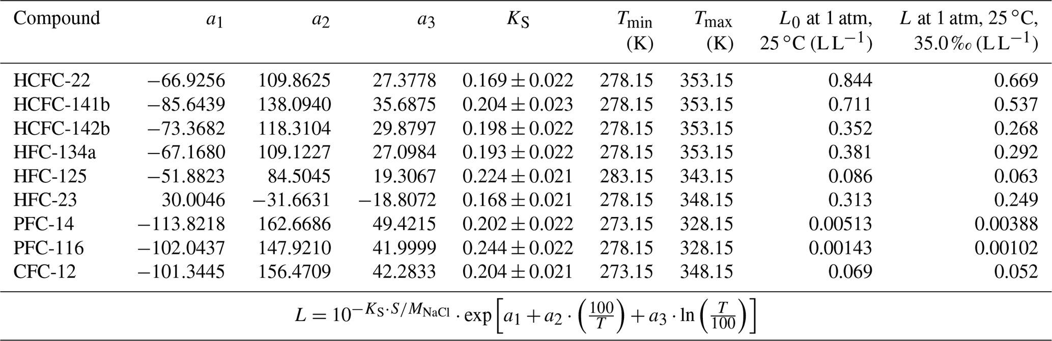
For PFC-14, the freshwater solubility curve in Ostwald solubility units (Fig. S2h) was compared with the ones from both Clever (2005) and Deeds (2008). The curve in this study matches better with the one from Clever (2005). In Fig. S2a-h, the fits for water solubility functions agree within 4.0 %, 7.8 %, 2.5 %, 6.8 %, 5.9 % 2.3 %, 0.95 % and 3.5 % with the majority (two-thirds) of the data for HCFC-22, HCFC-141b, HCFC-142b, HFC-134a, HFC-125, HFC-23, PFC-14 and PFC-116, respectively. The constants a₁, a₂, a₃ for the solubility functions of the target compounds in water are given in Table 5.

In order to validate the calculation method of water solubility, the solubilities for CFC-12 in water calculated by the combined method and by the method from Warner and Weiss (1985) were compared. Warner and Weiss (1985) estimated the freshwater and seawater solubility function of CFC-12 through experiments and a different model fit without using a salting-out coefficient. The freshwater solubility function of CFC-12 calculated by the combined method was constructed by collecting freshwater solubility data from the literature (Fig. S2i). The freshwater solubilities of CFC-12 from Warner and Weiss (1985) match data from other studies very well (the root mean square of misfit is 0.006). Moreover, the fits based on the function in Warner and Weiss (1985) and the CGW model in this study match very well (Fig. S2i). The average relative standard deviation (RSD) of water solubility estimated by the two methods for CFC-12 in the range of 273.15–313.15 K (0–40 ^∘C) is 0.17 %. This means that our method for estimating freshwater solubility is valid.

3.3.2 Salting-out coefficient

The salting-out coefficient K_S is independent of salinity and is a function only of temperature, which can be obtained from method I and method II in Sect. 2.7. In order to validate this, K_S was calculated by Eq. (16) (method II) based on the experimental results of the freshwater and seawater solubility of CFC-12 from Warner and Weiss (1985). The average of K_S is $\mathrm{0.229}\pm (\mathrm{1.41}\times {\mathrm{10}}^{-\mathrm{15}}$) L g⁻¹ at 298.15 K when the salinity is in the range of 0–40. The RSD is $\mathrm{6.16}\times {\mathrm{10}}^{-\mathrm{13}}$ %, which is minor enough to be neglected. Thus, K_S is independent of salinity. In Fig. S3, a quadratic relationship between the salting-out coefficient and temperature was found. K_S is in the range of 0.229–0.249 L g⁻¹ (at a mean of 0.235±0.005 L g⁻¹) at a salinity of 35 when the temperature is in the range of 273.15–313.15 K (0–40 ^∘C). The RSD is 2.3 %. This means that the effect of temperature on the salting-out coefficient is also very small.

In order to estimate the solubility functions for target compounds in seawater, their salting-out coefficients (K_S) should be estimated. As shown in Eq. (17), K_S is estimated based on the descriptors of all target compounds. With the exception of PFC-116, E, S, A, B and V_c values for the target compounds were obtained from Abraham et al. (2001, 2012). For PFC-116, the excess molar refraction (E) was calculated by Eq. (15). The dipolarity–polarizability (S) for PFC-116 (C₂F₆) was estimated as −0.350 based on the S of PFC-14 (CF₄, −0.250) and PFC-218 (C₃F₈, −0.450) (Abraham et al., 2001) and the error for the estimate of S is estimated to be 0.02 based on the error propagation. A and B for PFC-116 (C₂F₆) are both zero since it includes only carbon–halogen atom bonds and no carbon–hydrogen bonds. V_c of PFC-116 was obtained from Abraham and McGowan (1987) and Goss et al. (2006). The values of all descriptors for the target compounds are shown in Table 4. The errors in calculating the descriptors were estimated as 0.088, 0.047, 0.128, 0.081, 0.095, 0.051, 0.071 and 0.088 for HCFC-22, HCFC-141b, HCFC-142b, HFC-134a, HFC-125, HFC-23, PFC-14 and PFC-116, respectively (Abraham et al., 2001). On the basis of the E, S, A, B, V_c descriptors, salting-out coefficients (K_S) were estimated at 298.15±2 K and are shown in Table 5.

As shown in Sect. 2.7.2, K_S changes with temperature, which is described by the coefficients c, e, s, a, b and v in Eq. (17). The salting-out coefficient is a second-order polynomial function of temperature as we described for method I in Sect. 2.7.1 and discussed above for CFC-12 (Fig. S3). Based on the discussion for CFC-12, the effect of temperature on the salting-out coefficient is small. Also, very limited studies of K_S have been reported and we assume that the salting-out coefficient K_S does not change with temperature (i.e., it is a constant). Thus, the final salting-out coefficients are calculated using Eq. (17) at 298.15 K for the target compounds and shown in Table 5.

3.3.3 Solubility in seawater based on the combined method

Following the calculation method shown in Sect. 2.7.3, seawater solubility functions for HCFC-22, HCFC-141b, HCFC-142b, HFC-134a, HFC-125, HFC-23, PFC-14 and PFC-116 were constructed in the corresponding temperature range (Table 5) based on Eq. (19). Ostwald solubility coefficients in seawater at 1 atm, 25 ^∘C and 35 g kg⁻¹ were estimated to be 0.669 L L⁻¹ for HCFC-22, 0.537 (HCFC-141b), 0.268 (HCFC-142b), 0.292 (HFC-134a), 0.063 (HFC-125), 0.249 (HFC-23), 0.00388 (PFC-14) and 0.00102 (PFC-116), respectively (Table 5). For comparison, the solubilities of CFC-12, CFC-11, CFC-113, CCl₄ and SF₆ in seawater are converted to the Ostwald solubility unit at 1 atm, 25 ^∘C and 35 g kg⁻¹. They are 0.0504, 0.177, 0.0518, 0.568 and 0.00401 L L⁻¹, respectively. In previous studies, Mackay et al. (2006) reported that many hydrocarbons have a solubility in seawater ∼75 % of their solubility in distilled water. Moore et al. (1995) reported that the solubility of short-lived halocarbons (e.g., CH₃I, CHBr₃, CH₂Br₂, CHBr₂Cl and CHCl₃) in seawater is 80 % of their solubility in freshwater. For comparison, the solubility of CFC-12 in seawater is 73 % of its solubility in freshwater (Warner and Weiss, 1985). The percentages are 72 % for CFC-11 (Warner and Weiss, 1985), 74 % for CFC-113 (Bu and Warner, 1995), 78 % for CCl₄ (Bullister and Wisegarver, 1998) and 73 % for SF₆ (Bullister et al., 2002). For our target compounds, the percentages of seawater solubility for freshwater solubility at 298.15 K and a salinity of 35 % are 79 % for HCFC-22 and HFC-23, 77 % for HFC-134a, 76 % for HCFC-141b, HCFC-142b and PFC-14, 73 % for HFC-125, and 71 % for PFC-116. Similar to the CFCs and SF₆, the percentages for HCFCs, HFCs and PFCs are also in the range of around 70 %–80 %.

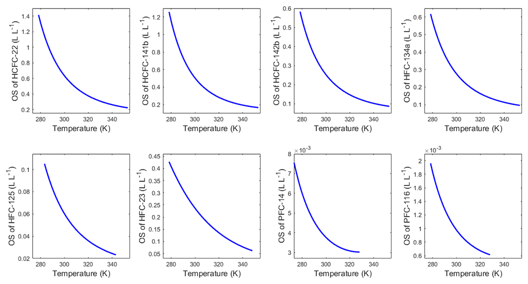
Figure 3 Temperature dependence of the Ostwald solubility (OS) coefficients in seawater for HCFC-22, HCFC-141b, HCFC-142b, HFC-134a, HFC-125, HFC-23, PFC-14 and PFC-116 at a salinity of 35.

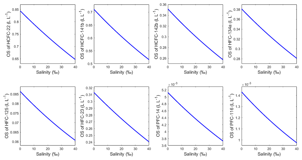
Figure 4 Salinity dependence of the Ostwald solubility (OS) coefficients in seawater for HCFC-22, HCFC-141b, HCFC-142b, HFC-134a, HFC-125, HFC-23, PFC-14 and PFC-116 at a temperature of 298.15 K.

The temperature dependence of the Ostwald solubility coefficients of the target compounds in seawater at a salinity of 35 is shown in Fig. 3. The dependence on salinity at 298.15 K is shown in Fig. 4. Seawater solubilities fall monotonically with increasing temperature and salinity. The latter shows a near-linear decline.

Overall uncertainties of water solubility estimates for the target compounds are calculated as the root mean square of the misfit between the measurements and the fitted values. They are 0.0352 L L⁻¹ for HCFC-22, 0.0283 (HCFC-141b), 0.0065 (HCFC-142b), 0.0141 (HFC-134a), 0.0016 (HFC-125), 0.0132 (HFC-23), $\mathrm{9.0695}\times {\mathrm{10}}^{-\mathrm{5}}$ (PFC-14) and $\mathrm{9.1858}\times {\mathrm{10}}^{-\mathrm{5}}$ (PFC-116). The uncertainties of seawater solubility of the target compounds at different salinities (0–40) and a temperature of 298.15 K are estimated by the propagation of uncertainty from water solubility and salting-out coefficients. They are 0.034 L L⁻¹ for HCFC-22, 0.032 (HCFC-141b), 0.031 (HCFC-142b), 0.031 (HFC-134a), 0.030 (HFC-125), 0.031 (HFC-23), 0.030 (PFC-14) and 0.029 (PFC-116). The uncertainties of seawater solubility at different temperatures (273.15–313.15 K) and a salinity of 35 are also estimated by the same method. They are 0.041 L L⁻¹ for HCFC-22, 0.037 (HCFC-141b), 0.029 (HCFC-142b), 0.030 (HFC-134a), 0.026 (HFC-125), 0.029 (HFC-23), 0.027 for (PFC-14) and 0.025 (PFC-116).

Table 6 Comparison of the Ostwald solubility coefficients (L, L L⁻¹) of PFC-14 in seawater with previous results.

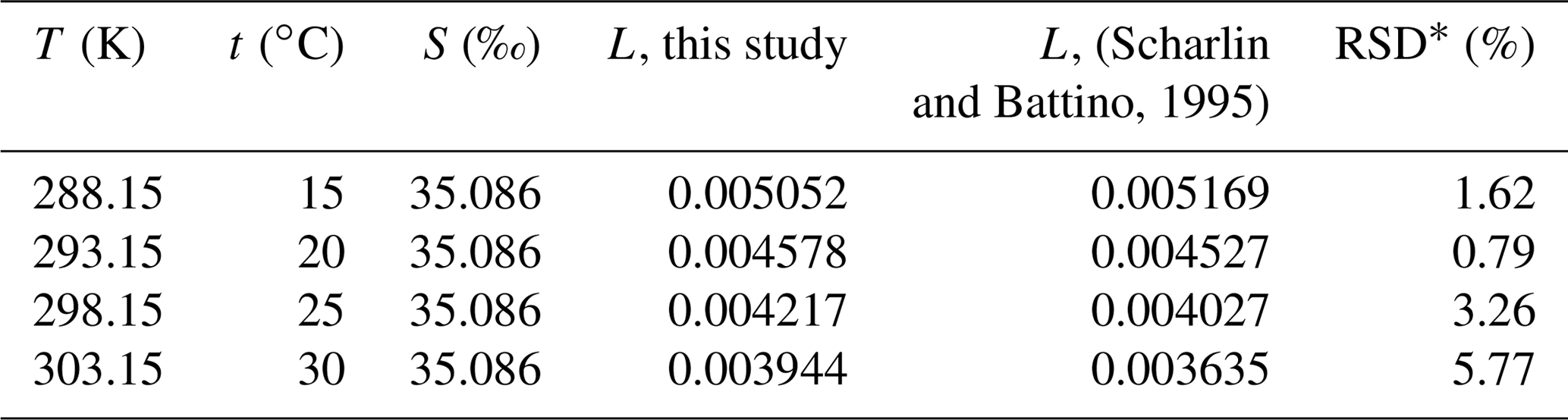
^* Relative standard deviation (RSD) of the Ostwald solubility coefficients estimated by the combined method and measured in Scharlin and Battino (1995).

In order to evaluate the effectiveness of the combined method, the Ostwald solubility coefficients of PFC-14 in seawater estimated by the combined method were compared with the observed values (Table 6) because only the seawater solubilities of PFC-14 have been measured (Scharlin and Battino, 1995). The estimated solubility of PFC-14 in seawater at 293.15 K is the closest to the measured values. The RSD of the calculated value and the measured value is only 0.79 %.

3.3.4 Comparison of solubility in seawater based on three methods

In order to validate the possibility of method I and method II, and to find out the advantages of the combined method, we estimated seawater solubilities of the target compounds based on method I and method II and compared them to the results from the combined method.

For method I, only the seawater solubility function of PFC-14 was constructed (Table S3) as only the seawater solubilities of PFC-14 have been reported (Scharlin and Battino, 1995). The advantage of the constructed seawater solubility function is that it can be used over a greater temperature range rather than only for a few selected temperatures.

The only difference between method II and the combined method is the difference in estimating water solubility. For water solubility calculations, method II uses the pp-LFERs based only on the physical properties of compounds, whereas the combined method uses the CGW model based on measurements. For water solubility based on the pp-LFERs, the water solubilities L₀ estimated by Eqs. (12), (13) and (14) based on V, log L¹⁶ and V_c were compared to the observed values (Table S4). As shown in Table S4, the water solubilities of most compounds calculated based on V_c (revised method II) are closer to both the observed values (Abraham et al., 2001) and the CGW fitted values than when they are calculated based on V or log L¹⁶ (method II). So the revised method II is more suitable for the target compounds except for HFC-125 for which the pp-LFER model method is used. The calculated water solubilities based on the (revised) method II are shown in Fig. S2a–i for comparison. Small differences in water solubility calculated by the (revised) method II and the combined method (CGW model) verify the reliability of both methods. Compared with the pp-LFER model method, the water solubility estimated by the CGW model method is closer to the observed values (Table S4). This is also the reason why the CGW model method from method I is chosen for the combined method in estimating water solubility coefficients. The final seawater solubility functions of the target compounds and CFC-12 based on (revised) method II are shown in Table S5.

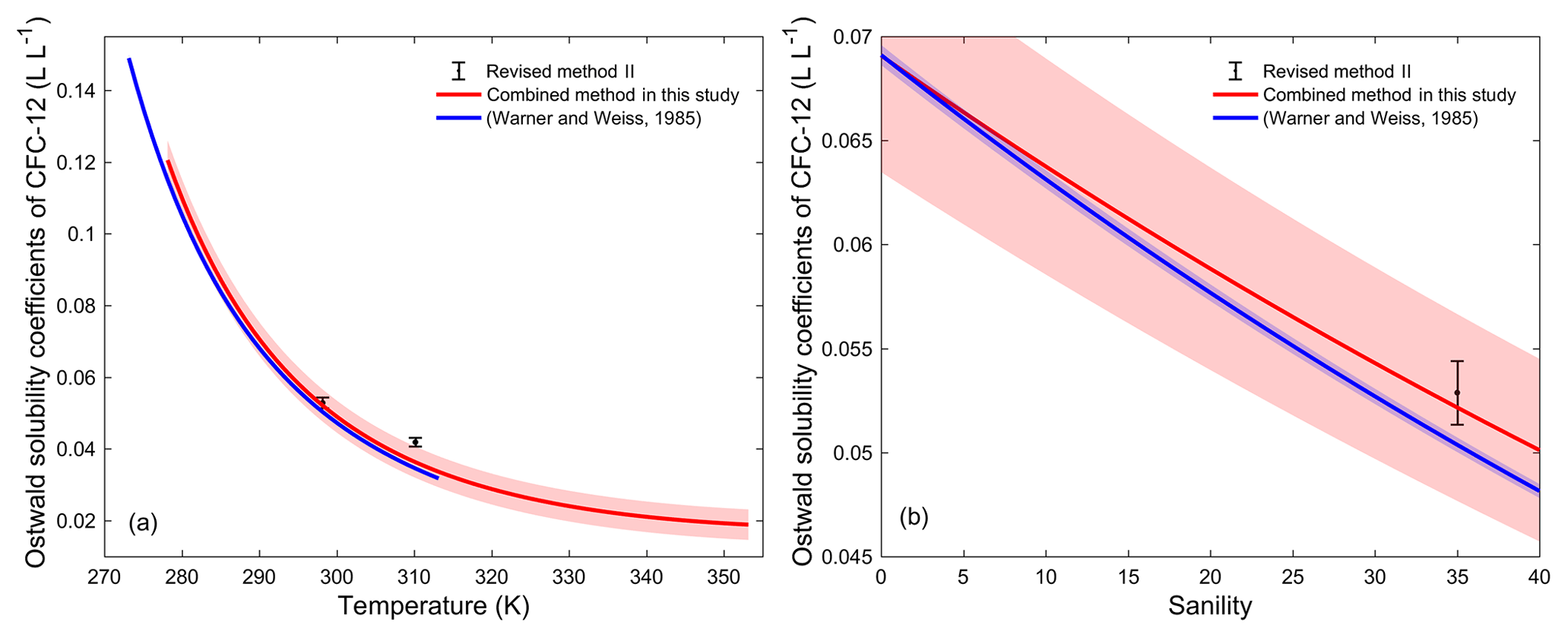
Figure 5 Comparison of the Ostwald solubility coefficients in seawater for CFC-12 (a) in the available temperature range at a salinity of 35 and (b) in the salinity range of 0–40 at a temperature of 298.15 K calculated from revised method II, from the combined method, and from Warner and Weiss (1985). Error bars and shadings in the figure reflect the uncertainties.

Until now, seawater solubility functions for the target compounds and CFC-12 based on (revised) method II and the combined method have been constructed. In order to better understand the difference between experimental results and model estimations, we compared the seawater solubility of CFC-12 calculated from Warner and Weiss (1985), from revised method II, and from the combined method. The results are shown in Fig. 5. The RSDs of the seawater solubility for CFC-12 estimated by the revised method II and by Warner and Weiss (1985) are 3.4 % at 298.15 K and 13.5 % at 310.15 K. The average RSDs of the seawater solubilities estimated by Warner and Weiss (1985) and by the combined method are 1.4±0.9 % in the coincidental temperature range of 278.15–313.15 K at the same salinity of 35 and 2.9±0.4 % in the coincidental salinity range of 0–40 at the same temperature of 298.15 K. These results show that the seawater solubility estimated by the combined method is very close to measured values in Warner and Weiss (1985). Without measurements of the seawater solubility of these compounds, the combined method is a good way to estimate the seawater solubility.

Based on the discussion above we make the following recommendations with respect to the calculation of the seawater solubilities of halogenated compounds.

• i.

  The (revised) method II could be used to estimate the seawater solubilities of compounds when neither water solubility data nor seawater solubility data have been obtained. This method is only based on the physical properties of compounds. The water solubility values and the salting-out coefficients are both estimated using the pp-LFERs.

• ii.

  The combined method is a better way to estimate the seawater solubility of compounds when water solubility, but not seawater solubility, has been measured. This is the case for the current study. The water solubility function is constructed based on the CGW fit and the salting-out coefficient is estimated using the pp-LFERs.

• iii.

  The method in published studies (Warner and Weiss, 1985; Bu and Warner, 1995; Bullister and Wisegarver, 1998; Bullister et al., 2002) is the best way to estimate seawater solubilities. Here, both the water solubility values and seawater solubility values are experimentally determined.

It is worth noting that these methods can potentially be applied to many more compounds.

3.4 Transient tracer potential and comparison with CFC-12

The production and consumption history of CFC-12 is shown in Fig. 1. The history of CFC-12 used as an oceanic transient tracer is also presented here. In 1973, Lovelock et al. (1973) first proposed that CFC-12 can be used as a transient tracer to study water masses in the ocean. Subsequently, large numbers of studies (Gammon et al., 1982; Weiss et al., 1985; Smethie et al., 1988; Körtzinger et al., 1999; Tanhua et al., 2008; Smith et al., 2016; Fine et al., 2017) using CFC-12 as an oceanic transient tracer have been published. In the 1990s, the World Ocean Circulation Experiments (WOCE) used CFC-12 as the normal tracer to investigate global ocean circulation and mixing. CFC-12 is still used as a tracer, although its production was prohibited in 1996; its atmospheric mole fraction subsequently peaked in the early 2000s and is now in slow decline.

As one of the requirements to be a useful oceanic tracer, transient source functions (i.e., atmospheric mole fraction histories) have been established for HCFC-22, HCFC-141b, HCFC-142b, HFC-134a, HFC-125, HFC-23, PFC-14 and PFC-116 here. With the exception of HCFC-141b (Fig. S1b) and HCFC-142b (Fig. S1c), the discussed compounds are still steadily increasing in the atmosphere. Therefore, they have the potential to be used as oceanic transient tracers if only considering their source functions.

For HCFCs, only mole fractions of HCFC-22 are continuing to increase in the global atmosphere. All three HCFCs show declining growth rates since 2007. Combined with the ban on HCFCs in 2007, freezing in 1996 (developed) to 2013 (developing) and the phaseout in 2020–2030 (Fig. 1), HCFCs can likely be used as oceanic transient tracers for the next several decades for recently ventilated waters. Due to a fall in emissions of HCFC-141b and HCFC-142b, the use of these two compounds will be more limited than HCFC-22 considering that atmospheric mole fractions of HCFC-141b have already begun to decrease and mole fractions of HCFC-142b are likely to decrease quite soon. Therefore, the atmospheric lifetimes of compounds are quite important, particularly once emissions have fallen. When atmospheric mole fractions of a given compound start to decrease, they are obviously no longer monotonically increasing, and the resultant calculated equilibrium atmospheric mole fraction in the ocean is no longer unique. Consequently, there will be two possible apparent ages for water masses so that this compound will have limited use as an oceanic tracer.

The mole fractions of HFCs are continuously increasing in the atmosphere, as are their growth rates. Restrictions on HFC consumption in the 2016 Kigali Amendment, with reduction of consumption beginning in 2019 in developed countries and freezing of consumption in 2024–2028 in developing countries (Fig. 1), mean that HFCs can likely be used as oceanic transient tracers for young waters for the next several decades. Moreover, HFCs have a higher potential to be oceanic transient tracers than HCFCs considering the increasing growth rates in the background atmosphere.

PFCs are increasing in the atmosphere over well-known natural background mole fractions. Combined with an atmospheric lifetime of over 50 000 years for PFC-14 and 10 000 years for PFC-116, PFCs have greater potential than HCFCs and HFCs to be oceanic transient tracers. PFC-14 has the potential to be a tracer for a longer period thanks to its longer lifetime, steady atmospheric growth rate and no current ban, as discussed by Deeds et al. (2008). However, PFC-14 is difficult to measure because it is extremely volatile and difficult to trap and separate chromatographically. PFC-116 can also be used as a transient tracer similar to PFC-14. The challenges for PFC-116 as an oceanic tracer are that it is a significant analytical challenge (low mole fractions in the atmosphere) with low solubility in seawater.

Well-established source functions and solubility functions in seawater are only two of the many requirements for an oceanic tracer. To be an oceanic transient tracer, the compound should also be conservative in the marine environment and be capable of rapid, relatively inexpensive and accurate measurement. The conservative nature of target compounds is briefly discussed in Sect. 1.2 by estimating the oceanic partial lifetimes of compounds with respect to hydrolysis in seawater. As we discussed for CFC-12, it is still used as an oceanic transient tracer though its production was phased out in the 1990s. For our target compounds, they have opportunities to be tracers once they are stable in seawater, can be measured in the ocean and have potential while atmospheric mole fractions continue to increase. This work provides two of the requirements for potential new oceanic transient tracers, while additional studies on compound conservation in seawater (comprehensive and detailed discussion) and measurement methods of target compounds are needed to qualify these compounds as suitable tracers.

4 Conclusions

This work has established the source functions for HCFC-22, HCFC-141b, HCFC-142b, HFC-134a, HFC-125, HFC-23, PFC-14 and PFC-116 based on a synthesis of available data and models optimized for transient tracer work in two ways: (1) the atmospheric mole fractions are calculated at the time of water mass formation (late winter in each hemisphere) and (2) the seawater solubility of these compounds is reviewed for the first time. In general, the mole fractions of most compounds have been continuously rising over the past 3 decades and are still increasing today (though HCFC-141b and 142b rise rates have slowed down significantly). For HCFC-141b and HCFC-142b the annual mean mole fractions show sigmoidal growth and the growth rates have the shape of a normal distribution. For HFC-134a and HFC-23, the annual mean mole fractions show initial exponential growth followed by linear increase and the growth rates show a sigmoidal pattern. For HFC-125, the annual mean mole fractions and growth rates both show an exponential increase. To a certain extent, these growth patterns could predict the trends of annual mole fractions in the near future. The source functions and natural background mole fractions for all compounds show that HCFC-22, HCFC-141b, HCFC-142b, HFC-134a, HFC-125 and HFC-23 have the potential to be oceanic transient tracers for the next few decades, though their growth rates are expected to reverse, particularly for the HCFCs, due to the restriction on production and consumption imposed by the Montreal Protocol. HFCs have a higher potential to be oceanic transient tracers than HCFCs due to the increasing growth rates in the atmosphere, though these are likely to fall as a result of the recent Kigali Amendment. PFC-14 and PFC-116 have the potential to be tracers for a longer period due to their longer lifetimes, more consistent atmospheric growth rates and lack of direct production or emission bans currently in place, though they are listed in the Kyoto Protocol and industrial practices are changing to try to reduce or minimize emissions. In addition, we have used three different methods to estimate the seawater solubilities of the compounds of interest based on available theoretical concepts and experimental data. The seawater solubility functions of these compounds were subsequently constructed, completing the input functions of these potentially useful oceanic transient tracers.