the Creative Commons Attribution 4.0 License.
the Creative Commons Attribution 4.0 License.
 | 04 Mar 2019
Use of a hydrodynamic model for the management of water renovation in a coastal system
Marta F.-Pedrera Balsells
Marc Mestres
Margarita Fernandez
Manuel Espino
Manel Grifoll
Agustin Sanchez-Arcilla
In this contribution we investigate the hydrodynamic response in Alfacs Bay (Ebro Delta, NW Mediterranean Sea) to different anthropogenic modifications in freshwater flows and inner bay–open sea connections. The fresh water coming from rice field irrigation contains nutrients and pesticides and therefore affects in multiple ways the productivity and water quality of the bay. The application of a nested oceanographic circulation modelling suite within the bay provides objective information to solve water quality problems that are becoming more acute due to temperature and phytoplankton concentration peaks during the summer period when seawater may exceed 28 ∘C, leading to high rates of mussel mortality and therefore a significant impact on the local economy. The effects of different management “solutions” (like a connection channel between the inner bay and open sea) are hydrodynamically modelled in order to diminish residence times (e-flushing time) and water temperatures. The modelling system, based on the Regional Ocean Modeling System (ROMS), consists of a set of nested domains using data from CMEMS-IBI for the initial and open boundary conditions (coarser domain). One full year (2014) of simulation is used to validate the results, showing low errors with sea surface temperature (SST) and good agreement with surface currents. Finally, a set of twin numerical experiments during the summer period (when the water temperature reaches 28 ∘C) is used to analyse the effects of proposed nature-based interventions. Although these actions modify water temperature in the water column, the decrease in SST is not enough to avoid high temperatures during some days and prevent eventual mussel mortality during summer in the shallowest regions. However, the proposed management actions reveal their effectiveness in diminishing water residence times along the entire bay, thus preventing the inner areas from having poor water renewal and the corresponding ecological problems.
Please read the corrigendum first before continuing.
-
Notice on corrigendum
The requested paper has a corresponding corrigendum published. Please read the corrigendum first before downloading the article.
-
Article
(989 KB)
-
The requested paper has a corresponding corrigendum published. Please read the corrigendum first before downloading the article.
- Article
(989 KB) - Full-text XML
- Corrigendum
- BibTeX
- EndNote


Coastal lagoons are highly productive areas, for instance regarding aquaculture, and are subject to multiple anthropogenic pressures. Due to the specific characteristics of these environments – e.g. small dimensions, calm inner waters, constrained exchange with open sea, heavy load of nutrients – there is usually a wide variety of problems related to water quality that can strongly limit their use and exploitation (e.g. HABs, anoxia–hypoxia events, water renovation or high seawater temperatures; Smith, 2003).
This problem is illustrated by the Ebro Delta coastal bays (NW Mediterranean) in which, for most of the year, there is an interaction between incoming saltwater from the coastal sea and fresh water discharged into the bays through the irrigation system from the surrounding rice fields. These discharges are rich in nutrients and pesticides (Köck et al., 2010), therefore affecting in multiple ways the productivity and water quality of the bays (Loureiro et al., 2009), in which residence times can be large depending on the prevailing met-ocean conditions (Artigas et al., 2014).
These bays (Alfacs in the south and Fangar in the north hemidelta) constitute the most important shellfish aquaculture area on the Spanish Mediterranean coast. They are considered very productive coastal areas compared to the oligotrophic western Mediterranean Sea; the primary production per volume unit is 1 order of magnitude greater than in the adjacent open sea (Delgado, 1989) and their waters support important fisheries and mussel and oyster cultures. Moreover, the economy of the area is largely based on activities that depend on primary production, such as agriculture, fisheries and aquaculture. The shellfish aquaculture in the region has to face different types of risks: shellfish pathogens (López-Joven et al., 2015), extreme warm events in the last years (Fernández-Tejedor et al., 2010), contamination (Köck et al., 2010), HABs and toxin accumulation (Loureiro et al., 2009), and the proliferation of invasive alien species, for example tunicates (Ordóñez et al., 2015). Water mass transport in marine systems has been demonstrated to be a decisive factor controlling the behaviour of chemical and biological variables of the ecosystem (Wolanski, 2007). In this sense, the evolution of the ecological status of the bays is highly related to water renewal and substance dispersion. Wind- or wave-induced resuspension processes may also affect the ecological status by inducing the vertical transport of substances from the sea bottom to the inner water column (Umgiesser et al., 2004).
The application of a nested oceanographic model with enough resolution to solve the inner dynamics of this kind of environment provides objective information to address water quality problems. These are becoming more relevant in the Ebro Delta bays due to increasing peaks of temperature and nutrient concentrations during the summer when seawater may exceed 28 ∘C, leading to high rates of shellfish mortality and therefore having a significant impact on the local economy.
In this contribution, focused on Alfacs Bay, we explore the suitability of land boundary conditions and the controlling effect of different management actions on the resulting 3-D circulation patterns based on renewal times. In this context, we also discuss the implications of opening a connection between the open sea and the inner bay, dredging the sandbar, and how it affects water temperature and concentrations. This has been a long-standing proposal by local fishermen to enhance water renovation rates and improve the water quality within the bay. A set of 3-D numerical model simulations spanning 1 year (2014), with outer boundary conditions from Copernicus Marine Environment Monitoring Service (CMEMS) models, is compared to intensive field campaigns and discussed in terms of water renovation and temperature. The implications of a hydraulic connection to the outer sea is analysed as a natural and sustainable type of intervention. From here, a set of conclusions on the models' performance and on the effectiveness of such sustainable intervention are presented.
2.1 Study area
Alfacs Bay is part of the Ebro Delta, which extends about 25 km offshore and forms two semi-enclosed bays on its lateral margins, Alfacs to the south and Fangar to the north. Both bays receive direct freshwater input from the drainage channels of nearby rice fields. In Alfacs Bay, these freshwater inputs are distributed in two dominant periods: from April to December with mean flows estimated by Llebot et al. (2011) of around 10 m3 s−1 and from January to March with channels closed and flows around 1 m3 s−1 (hereinafter referred to as wet and dry periods, respectively) due to rain and groundwater sources. Alfacs Bay is about 16 km long and 4 km wide, with a 2.5 km wide mouth, an average depth of about 4 m, and a maximum of 6.5 m in the middle of the bay. Figure 1 presents the location and bathymetry of the bay. The bay is closed in the east by a sandbar beach called Trabucador bar. This coastal barrier linking the main lobe of the Ebro Delta with its southern spit has suffered various breaching events associated with storms, opening an ephemeral connection between the bay and the open sea (Sánchez-Arcilla and Jiménez, 1994; Gracia et al., 2013). The bed is mostly muddy (largest percentages in the middle of the bay) with silty sediments present close to the freshwater outflows (Palacín et al., 1991).
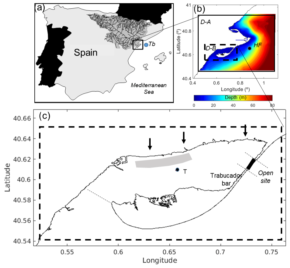
Figure 1Location of Ebro Delta, Alfacs Bay and PdE Tarragona buoy (blue point, Tb) (a). (b) The nesting scheme with the coastal (D-A) and bay (D-B) domains and bathymetry. Data from HF-R used to validate the system are indicated as “HF” (0.91∘ E, 40.31∘ N). (c) Location of the weekly CTDs (T). The opening area of the Trabucador bar modified in the numerical experiments is also shown. The dashed line in the bay mouth indicates the separation between the inner bay and open sea for the salinity box model. The grey rectangle indicates the mussel farm area. The freshwater drainage channel locations are indicated with arrows.
The bay has been defined as a salt-wedge estuary with an almost year-round stable stratification, alternated with well-mixed periods directly related to strong wind (Camp and Delgado, 1987) or seiche events (Cerralbo et al., 2015). Solé et al. (2009) found that drainage discharges were the main factor controlling the observed stratification. Cerralbo et al. (2015) found that during warm periods the salinity distribution shows strong vertical gradients, coinciding with isopycnals, with the saltiest water (almost 38) from the outer sea in the deepest mouth layers and the freshest water (35–36) at the surface. Stratification is weaker in the inner bay, with lower salinity values in the water column. Within the bay, fresh water at the surface layer extends from the northwest to the southeast with a pycnocline at 3–4 m of depth (Camp, 1994; Llebot et al., 2011). The water temperatures during summer show a clear diurnal pattern, with a clear stratification. This pattern occurred until the end of summer, when strong, dry and cold winds from the NW mix and cool the water column (Cerralbo et al., 2015; Grifoll et al., 2016). In Llebot et al. (2011), annual cycle (and inter-annual) analyses of temperature, salinity and some ecological indicators are described. Moreover, Llebot et al. (2014) use the Wedderburn number to identify wind events with enough energy to modify stratification, defining the mixed layer deepening response to wind events. Cerralbo et al. (2014) studied the tidal characteristics of the bay, noting the importance of the 3 h seiches and describing the 1 h seiches (corresponding to the first seiching mode). The subtidal patterns have been related to estuarine circulation (Llebot et al., 2014) and wind influence through empirical orthogonal function (EOF) analysis (Cerralbo et al., 2019). On the other hand, several ecological studies noted the presence of harmful algal blooms (HABs) in some periods and their relation to nutrients and waters from the open sea (Loureiro et al., 2009). Ramón et al. (2007) and Fernández-Tejedor et al. (2010) have reported mussel mortalities associated with high seawater temperature in the Ebro Delta bays.
Table 1Summary of observations (see Fig.1 for identifications).
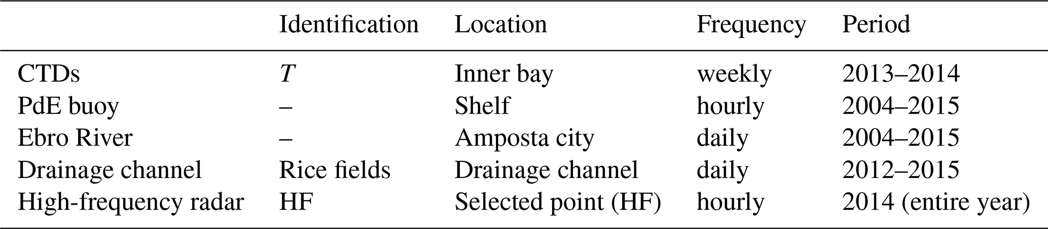
2.2 Observations
Weekly conductivity–temperature–depth (CTD) profiles were conducted in the framework of the monitoring programme for toxic phytoplankton in shellfish growing areas during the years 2013–2014. The location of one sampling station is shown in Fig. 1 (T). The water temperature in different locations (and representing different kinds of waterbodies) of the region is summarized in Fig. 2. The water temperatures inside the bay (T) and in the drainage channels are very similar (low gradients between them). The lowest temperatures (∼10 ∘C) occur during the winter season (December to March). After this, a gradual rise in water temperature is observed, with maximum values around 29 ∘C during summer (June to August). Finally, the water temperature decreases, affected by the influence of NW strong, dry and cold winds. On the other hand, the water temperature from the river does show remarkable differences (mainly during summer), with gradients around 2–3 ∘C (similar to the coastal waters measured at the Tarragona coastal buoy) compared to inner-bay waters. All the observations are summarized in Table 1.
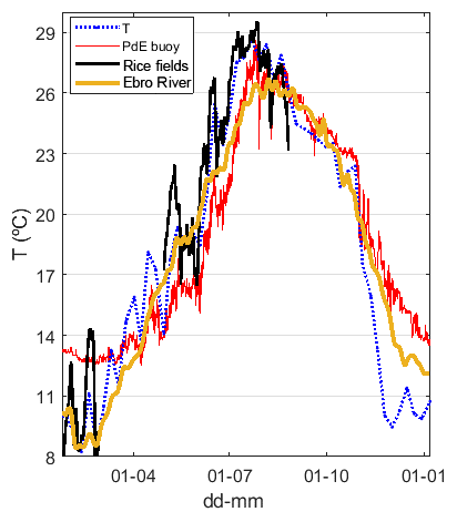
Figure 2Water temperatures in Alfacs Bay at point T (year 2014), drainage channels (rice fields, from climatological observations for 2002–2010 in a nearby coastal lagoon by the staff of the Ebro Delta Natural Park), Tarragona buoy (Tb) for open seawater conditions (Puertos del Estado, PdE) and climatological data from the Ebro River (Confederación Hidrográfica del Ebro).
2.3 Numerical model
The three-dimensional hydrodynamic model used in this study is the Regional Ocean Modeling System (ROMS). Numerical aspects are described in detail in Shchepetkin and McWilliams (2005), and a complete description of the model, with documentation and code, is available at the ROMS website: http://myroms.org (last access: 15 December 2018). Previous implementation for the model in Alfacs Bay showed a good skill assessment compared to currents, sea level and water temperature variables (Cerralbo et al., 2016).
The model applications consist of two nested regular grids with spatial resolutions of ∼350 and ∼70 m for the coarser (D-A) and finer domains (D-B), respectively (Fig. 1). The nesting ratio (∼5) between the two domains is defined to get enough resolution to reproduce the circulation in the inner bay, allowing for the transfer of large-scale dynamics into the nested domain. The nesting is offline; a first D-A simulation is performed and the hourly results are used for the boundary conditions of D-B. The chosen vertical discretization consists of 20 and 15σ levels for the coastal and bay domains, respectively. Bathymetries of the coastal system are built by combining bathymetric data from GEBCO (https://www.gebco.net/, last access: 2 December 2018) and specific local high-resolution sources. The bottom boundary layer is parameterized with a logarithmic profile using a characteristic bottom roughness height of 0.002 m. A surface stretching parameter (7.0) and bottom stretching parameter (0.4) for the Song and Haidvogel (1994) stretching function is used. This configuration allows for an increase in the resolution in the upper layer where the surface boundary layer is located due to the wind action. The transformation function used is described in Shchepetkin and McWilliams (2005) denoted as an unperturbed coordinate system. In order to represent the processes at scales smaller than the grid resolution we selected anisotropic horizontal and vertical turbulent schemes based on a generic length scale (GLS) formulation (Warner et al., 2005). K-ε parameters are chosen for GLS formulation. Also, the Kantha and Clayson stability function formulation is used (Kantha and Clayson, 1994). For the advection scheme a third-order upstream horizontal flux is selected. For heat and mass tracers, a biharmonic mixing scheme along geopotential surfaces is used.
A 1-year-long base simulation (hereafter referred to as BS, from 1 January to 31 December 2014) has been performed in order to validate the model and obtain the initial and boundary conditions for the 3-month simulations in the analysis period (summer 2014) in the smaller domain. The BS is done using the first 24 h of the CMEMS-IBI (Sotillo et al., 2015) daily forecasts for the initial and open boundary conditions. Hourly depth-averaged water currents and sea level are provided by CMEMS-IBI and consistently accommodated to the open boundaries (OBC) with Chapman and Flather algorithms (Carter and Merrifield, 2007). The variability of currents along the water column (3-D component), temperature and salinity are imposed from CMEMS-IBI daily average values with clamped conditions.
At the sea surface, the models are driven by high-frequency (hourly) wind components (with 0.05∘ resolution), atmospheric pressure, humidity, precipitation and solar radiation derived from the Spanish Meteorological Agency (AEMET) forecast (model HARMONIE). The wind stress and sensible and latent heat are computed internally by the model using aerodynamic bulk formulas. To avoid land contamination of the atmospheric forcing on coastal areas (e.g. heat fluxes and winds), a prior land mask is applied to the forcing data, and then variables over the sea are interpolated on the land. The freshwater flows are 1 m3 s−1 during January–March (dry season) and 10 m3 s−1 during April–December (wet season) distributed in the three channels (see Fig. 1c). Salinity is set to 18, and water temperature is defined from climatological water temperature in the Ebro River (Fig. 2).
For the sake of understanding the influence of land discharges and layout modifications on the water dynamics, a set of 3-month-long numerical experiments is done (1 June–30 September). In all of them, a passive tracer with a 1 kg m−3 concentration is initially released at all the computational nodes inside the bay. The BS simulation is restarted on 1 June with the passive tracers and is used as a control simulation (called C) to compare all the numerical tests. A second set of three tests has been prepared to understand the effects of establishing an artificial connection with the open sea through the Trabucador bar (see Fig. 1). This is an engineering action proposed in the last years by the local authorities to consolidate the ephemeral connection between the bay and the open sea that occurs occasionally due to storm-related bar breaching. The purpose of a permanent open sea connection is to solve the problems of the bay linked to long residence times and overheating, and similar solutions have been studied in other coastal lagoons with water quality issues (Netto et al., 2012; Lill et al., 2012). These simulations consist of opening the bar using different widths, from 200 to 800 m, and studying the effects on water renewal and sea surface temperature. Finally, two more numerical tests are performed in which the freshwater input flows were modified. Considering that the gravitational circulation in the bay has been previously related to the hydrodynamics of the bay (Cerralbo et al., 2019), it is expected to find variability in the water renewal times when the freshwater flows are modified. These numerical tests are designed to understand their effects on current patterns. In test R1 the usual flow (10 m3 s−1 in C) is doubled, keeping the proportion in the three channels. In test R2, the total discharged flow is doubled, but the flow increment is only applied to the innermost channel, while the outflow through the drainage channels closest to the bay mouth is kept the same as in C. Thus, the R1 test doubles the freshwater input along the three channels, and R2 only modifies the innermost channel. All the numerical tests are summarized in Table 2.
Table 2Numerical experiments and main characteristics.
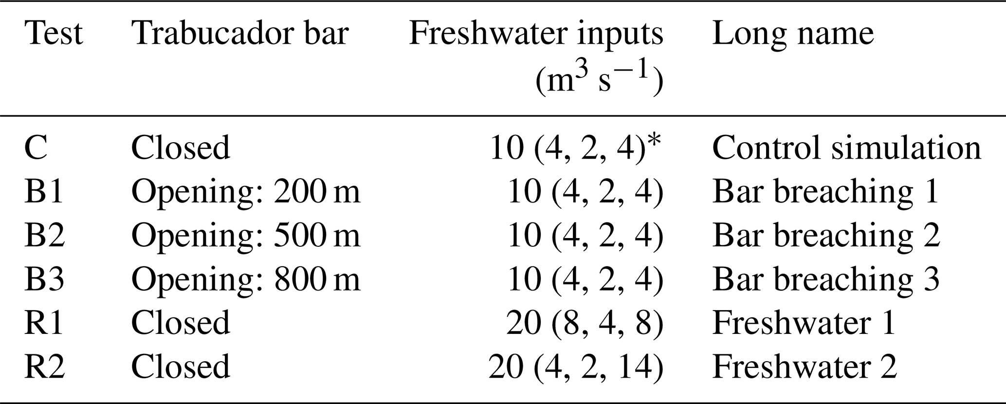
* The order inside the brackets indicates the location of a drainage channel from west to east (see Fig. 1).
2.4 Validation
Data from CMEMS-IBI, atmospheric models and field observations (high-frequency radar (HF-R) from Puertos del Estado, PdE), as well as sea surface salinity (SSS) and sea surface temperature (SST) data from the Institute of Agriculture and Food Research and Technology (IRTA), were available for the year 2014. The modelled and observed SSTs are shown in Fig. 3. A qualitative and quantitative comparison shows good agreement between the two variables (correlation of 0.99), with a small overheating in the modelled results (see statistics in Fig. 3). The errors in modelled SSS are mainly related to the uncertainty associated with the flows and the exact location of the discharge points. However, the results of the coastal model (D-A), which considers the inner-bay freshwater flows, show a closer agreement with the observed values than the CMEMS-IBI results, which do not account for the inner discharges. The variability of SSS in the CMEMS-IBI fields is related to the Ebro River plume, not to the influence of inner-bay freshwater inflows. Water surface currents are validated for the coastal model (D-A) considering the information from HF-R in the area (Lorente et al., 2016). The HF-R (CODAR SeaSonde standard range) was deployed at the Ebro Delta in 2013 within the framework of the RIADE (Redes de Indicadores Ambientales del Delta del Ebro) project. The network consists of three remote shore-based sites providing hourly radial measurements with a cut-off filter of 100 cm s−1 and representative of current velocities in the upper first metre of the water column (Lorente et al., 2015). The total current vectors are hourly averaged on a predefined Cartesian regular grid with 3×3 km horizontal resolution. The parent model (CMEMS-IBI) has been validated in the region using HF-R in Sotillo et al. (2015). Their results shows zonal and meridional root mean square error (correlation) values in the range of 6–10 cm s−1 (0.4–0.8) over central areas of the HF-R radar domain, with higher errors detected at the far edges of the radar spatial coverage (Sotillo et al., 2015). For D-A domain both eastward and northward components of the surface currents are shown in Fig. 3a and b (at point HF, location shown in Fig. 1). Validation is performed for all of 2014 in one point close to the bay and with optimal temporal coverage (more than 85 % of 2014 with data). The gaps in the HF-R data are not considered. The agreement and correlation between modelled and observed currents are very high (∼0.7), both in intensity and phase and in both components. The daily oscillations correspond to the inertial period in the region (∼19 h) and are well reproduced by the model. Some currents intensifications, probably related to energetic wind events, are also well described by the model (for instance on 10 February and 16 March).
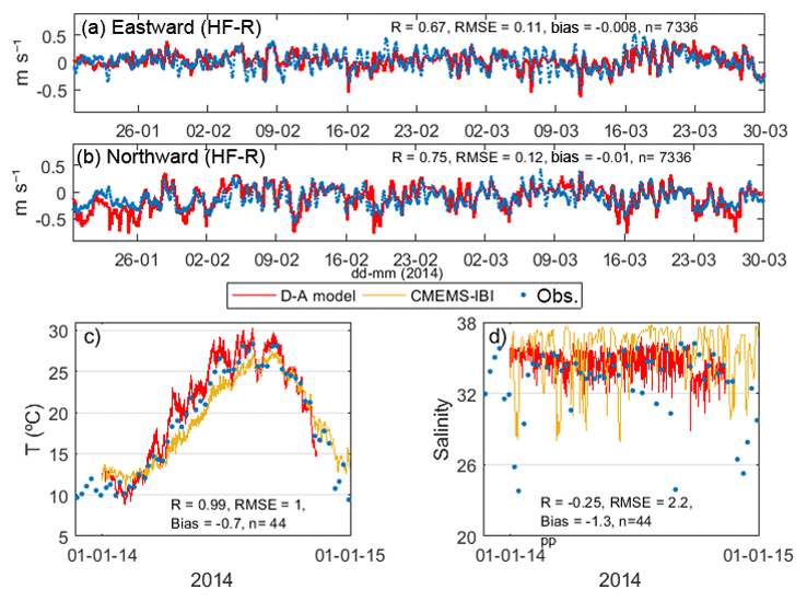
Figure 3Eastward (a) and northward (b) water surface currents for the D-A model and HF-R at HF (Fig. 1) are shown. SST (c) and SSS (d) validation of the local model D-B (red), CMEMS-IBI (yellow) and observations (blue) at T (Fig. 1).
2.5 Water residence times
There are a multitude of different methods and concepts to calculate water renovation in the literature. For any given domain, the simplest way to assess water renovation is to obtain the water exchange time through the ratio between its total volume (V) and the daily flux (Q) entering or leaving through its open boundaries. It represents the time required for the entire mass of water to be replaced by input water (Takeoka, 1984; Jouon et al., 2006). On the other hand, the e-flushing time (Thomann and Mueller, 1987) assumes that a passive tracer is injected into a homogenous water mass at time t with an initial concentration C0. The e-flushing time is the time required for the tracer mass initially contained within the whole domain to decrease by a 1∕e factor. A fair adaptation to this parameter, the local e-flushing time, is presented in Jouon et al. (2006) by considering the spatial variability of the e-flushing time and taking into account the evolution of the tracer in each cell of the computational mesh.
The integral water exchange time in Alfacs Bay can be grossly estimated using simple approaches. A first approximation can be done by considering the residual circulation presented in Cerralbo et al. (2018); through an analysis of the mean circulation the authors obtain residual velocities at the bay mouth. Using the mean residual currents and the bay's volume and typical cross section at the mouth leads to water exchange times (θ) of around 20 and 70 days for the wet and the dry season, respectively. Similar results can be also obtained using a box model approximation (Officer, 1980) based on the salinity variations between the bay water and the open sea with four layers: seaside surface and bottom (salinity of 36.35 and 37.82, respectively) and inner-bay surface and bottom layers (with salinities of 35.7 and 36.94). The box model is described by Eqs. (1–4).
Q is the total freshwater input, Si is the salinity in layer i, and Qij and Eij are the advective and turbulent fluxes between layers i and j. In this model, Q is set to 10 m3 s−1, and the salinities are given by the mean values obtained in the field campaigns described in Sect. 2.2. Solving the system with these values yields residence times of ∼13 and ∼40 days for the wet and the dry season, respectively. However, these methods are not useful when large variations in hydrodynamics occur (Jouon et al., 2006). In this sense, previous studies on the Alfacs Bay hydrodynamics have highlighted the relevance of hydrodynamic spatial variability associated with seiches (Cerralbo et al., 2014), winds (Llebot et al., 2014; Cerralbo et al., 2016) and gravitational circulation (Artigas et al., 2014).
An approximation to the spatial variability of the residence times is addressed for the first time in this work by analysing the space distribution of the local flushing time (LFT) for the entire waterbody. The methodology applied is based on the numerical deployment of an Eulerian conservative tracer, within the inner domain of the bay, to compute the time required for its concentration in each grid cell to decrease by a factor e−1 from the initial value. This definition represents the sum of the flushing lag and local e-flushing time in Jouon et al. (2006). Thus, an Eulerian passive and conservative tracer with a concentration equal to Co=1 kg m−3 was deployed in the different sigma layers of the inner bay. Considering that the pycnocline is around 3–4 m of depth (Camp, 1994) and mussel farms are mostly above this depth, the analysis focuses on the surface layers. The freshwater inflows are considered clean of the tracer. An example of the time evolution of the surface tracer concentration at two points is shown in Fig. 4a. The LFT is defined at each grid cell based on the concentration decrease between Co and using the best-correlated exponential regression (Jouon et al., 2006).
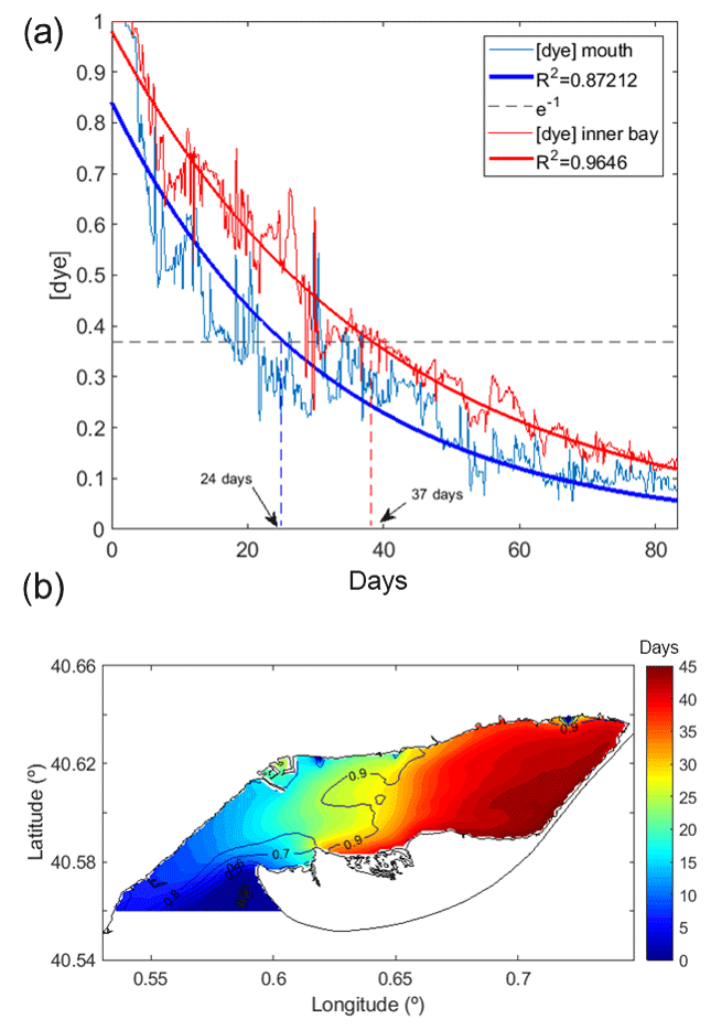
Figure 4(a) Time evolution of the dye concentration at two points – at the bay mouth and inside the bay – and the corresponding exponential fitting (with the squared correlation shown in the legend) used to obtain the LFT for the C case. (b) The local e-flushing time for the C case (colour). The black contour shows the squared correlation obtained at each of the grid points.
The results for LFT in the C simulation reveal a high spatial variability (Fig. 4b), with short values between 5 and 20 days in the region close to the bay mouth and near the freshwater discharges. These are similar to those presented in Camp (1994) and Llebot et al. (2011). On the other hand, longer times are found in the inner regions (30–47 days). When the total flushing time (TFT) is considered (TFT being equal to the period necessary for the average concentration of the entire bay to go from Co to ), values of about 28 days for C are found.
Table 3TFT values for the surface e-flushing time in the Alfacs Bay.
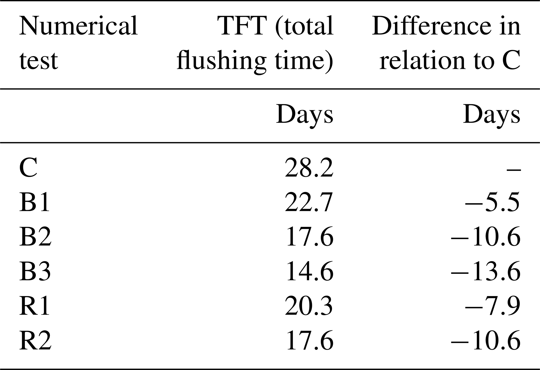
As mentioned before, the hydrodynamics of Alfacs Bay are particularly affected by freshwater inputs. Both R1 and R2 reveal (not shown) maximum LFT values of 34 and 29 days, respectively (shorter than C, with 47 days). The anomaly – in days – of these patterns in relation to the distributions obtained for C is shown in Fig. 5a and b. R1 shows shorter residence times than the C test in the innermost part of the bay. The clearest effects of the freshwater increment are observed in the area closest to the drainage points (with LFT under 10 days). However, the inner areas still present residence times longer than 30 days. The R2 results also show remarkable differences compared to the control case, with shorter times in the area close to the inner channel and values around 20 days in the innermost region. In both tests, the area of mussel farms shows similar differences, with LFT values almost 10 days shorter in the results obtained with modified freshwater flows. In Table 3 the TFT for the entire bay is summarized for all the cases. It is interesting to note that the TFT for test C is around 28 days, similar to the values obtained through the simple relation between the mean residual circulation and the volume of the bay. Tests R1 and R2 show a noticeable decrease in the average e-flushing time, with reductions of ∼8 and ∼11 days, respectively.
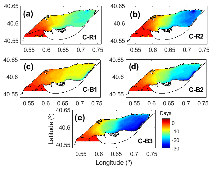
Figure 5Differences (in days) for the water e-flushing times between each test case and the control simulation (C). Negative (positive) indicates shorter (longer) local e-flushing times for the corresponding test compared with C.
Regarding SST (Fig. 6), the differences are evident, but not significant. In general, there is a cooling of the surface water over the entire bay of about 0.5 ∘C, being more evident in the vicinities of the drainage points. However, in the region near the Trabucador bar, the surface waters show an increase in temperature. This area is very shallow and probably the effects of higher stratification (induced by the highest freshwater inputs) and longer residence times in this region contribute to increasing the SST. Considering the integrated SST values for the entire bay, the R1 and R2 tests show a decrease of 0.07 and 0.08 ∘C in relation to the control test.

Figure 6Differences for the SST between each test case and the control simulation (C). Blue indicates a lower SST for the corresponding test compared with C (red indicates a lower SST for the control simulation).
To evaluate the effect of bar breaching, a set of three numerical tests (B1, B2 and B3) with different widths of sandbar breaching (200, 500 and 800 m, respectively) has been implemented. In all the cases, the depth of the channel is equal to the minimum depth considered in the model (1 m). Figure 1 shows the region of the sandbar modified for these simulations.
The results are summarized in Figs. 5 and 6. Test B1 (200 m) shows shorter LFT mostly in the region close to the sandbar. However, no remarkable differences are observed in the mussel farm region (differences of about 5 days with respect to C). Tests B2 and B3 (500 and 800 m) reveal a higher variation in the residence times than B1, but with similar spatial variability patterns. In general, a wider connection with the open sea implies a larger area with lower LFT in the vicinities of the sandbar and inner region. Moreover, the effects are also observed in the region of the mussel farms, with a decrease in the residence time to less than 10 days. The TFT for the entire bay and the differences relative to the C test are summarized in Table 3. There is clearly a direct relationship between the width of the channel and the residence times, with those for B3 (widest channel) being almost 14 days shorter than those for the control case C.
The analysis of SST differences shows no relevant discrepancies with the C case in most of the bay. Only the region closest to the open channel in the bar shows a decrease in the inner-bay SST (due to mixing with the cooler open seawater, as observed in Fig. 2) and also an increase in SST in the open seaside of the bar. The integrated values over the bay do not show significant variations between the tests and the control case, with differences smaller than 0.07 ∘C.
Previous studies had applied numerical models in Alfacs Bay (Llebot et al., 2014; Artigas et al., 2014; Cerralbo et al., 2014, 2015, 2016), trying to characterize the main hydrodynamic features of the bay: wind, sea level, seiches, mixing and gravitational circulation. However, none of them addresses one of the most relevant problems inside the bay related to low water renovation and warm water temperatures during summer periods. For this, a high-resolution numerical model able to simulate interventions and impacts has been implemented for the first time in the bay using the available data from CMEMS numerical models (as initial and boundary conditions) and following the nesting scheme designed in the SAMOA initiative (Sotillo et al., 2019). The validation of such an implementation with the available data in the coarser domain has been done through comparison with HF-R water surface currents, revealing very good performance and agreement. The validation of the higher-resolution domain – local – has been performed using SST and SSS from in situ field campaigns, revealing a good agreement between observed and modelled data for the SST. Errors in salinity could be related to the lack of accurate data for freshwater flows (total volume, spatial and temporal distribution) and the salinity of these waters (fresh water from rice fields mixed with brackish waters from the coastal lagoon). The model presented in this paper could be also considered as the first attempt towards the implementation of an operational system in the bay as a local downscaling of CMEMS products, which could be used by local authorities to improve the management of the bay. However, this study has revealed the scarcity of information about the bay, which may influence the robustness of modelling results. Lacking data include, for instance, accurate information on bathymetry, which is expected to improve with new products derived from Sentinel-2, and the correct characterization of the freshwater flows (i.e. number and spatial distribution of sources, water flows, and temperature).
As stated by several authors (i.e. Braunschweig et al., 2003; Jouon et al., 2006; Dabrowski et al., 2012; Grifoll et al., 2013) there are various ways to obtain the residence time of a given waterbody. In this contribution, we have followed different approximations, from a simplistic scheme using the observed residual velocities or the application of a box model that uses the salinities and freshwater flows to obtain the gravitational circulation, to the most complete scheme using the depletion of Eulerian conservative tracers in a numerical model (LFT and TFT). The analysis has focused on surface layers (above the pycnocline at 3–4 m) where the water column is entirely mixed. The water exchange times reveal values of 13 and 40 days for wet and dry periods, respectively, using the box model, similar to those obtained using residual currents (20 and 70 days). These results are in agreement with previous studies (Camp and Delgado, 1987; Llebot et al., 2011) presenting residence times for the Alfacs Bay between 10 (wet period) and 25 days (dry period). The differences between these results and previous studies may be due to the arbitrary selection of the bay mouth section, sensitivity to salinity and freshwater flows used in the box model, and the location of the current meters. In this sense, the variability of the flow through the mouth section has been demonstrated to be high in Cerralbo et al. (2016). However, simple methods consider all water particles to have the same transit time through the entire control volume (Takeoka, 1984). In Alfacs Bay, several authors (Llebot et al., 2011; Cerralbo et al., 2014, 2015, 2016) have observed remarkable variability in the spatial distribution of the hydrodynamics fields. Thus, the application of LFT allows for an understanding of the spatial variability of the residence time inside the bay and offers a proper information tool for the local authorities. The results of the LFT method reveal differences in renewal times among different areas (for instance, where the mussel farms are located) with residence times (LFT) around 15–20 days and regions inside the bay with much larger residence times (∼40–45 days). According to these data, the location of the mussel farms could be considered optimal when the residence time is considered. Only locations closer to the bay mouth show higher ratios of renovation. These results agree with an approximation by Artigas et al. (2014).
Once the numerical model is implemented, calibrated and validated, it can be used to test different interventions directed to improve the water quality of the bay. Considering that some of the main problems of the bay are related to the long residence times (i.e. anoxia as observed by Camp et al., 1992) and the high values of water temperatures during summer, several management options have been tested to find the best option to mitigate these negative effects. Two actions are proposed and analysed here: the modification of freshwater flows (both volume and spatial distribution) and the artificial connection with open sea through the El Trabucador bar. Both actions show a remarkable reduction in the LFT (and corresponding TFT), mostly concentrated in the inner area of the bay, with LFT in B3 and R2 almost half of that observed in C case, as noted in similar studies by Netto et al. (2012) and Lill et al. (2012). Previous studies have pointed out the presence of a region in the northeast of the bay with low residence times (Cerralbo et al., 2019), also described as a nutrient accumulation area (Artigas et al., 2014). The LFT shows noticeable spatial variability, with highest diminution in the region close to the artificial channel (in B1, B2 and B3) and the freshwater discharge points (R1 and R2). The region where the mussel farms are located also shows lower LFT than in the control case (reductions ranging from 20 % in B1 and R1 to 30 % in B3 and R2), but the differences are not as high as those observed in the inner bay. The effects of opening a ∼1 km wide channel (B3) are negligible in comparison to modifying the freshwater flows in R2 (increase in fresh water mainly concentrated in the inner channel). In that sense, the modification of the freshwater flows seems more feasible both economically and technically compared to artificially opening and maintaining a new connection with the open sea. Moreover, the opening of the sandbar would imply high economic (dredging, jetties) and environmental costs (breaking of alongshore circulation and transport of sediments and nutrients) that must be evaluated cautiously.
The water temperature from the drainage canals used in the simulations corresponds to the climatological values observed in the Ebro River, not to the observations in the drainage channels, which is similar to the temperature of the water inside the bay (see Fig. 2). This is because the channel freshwater input would not decrease the temperature of the bay water, but there is the possibility of doing this by conducting cooler water from the river directly to the bay using an irrigation system. However, none of the analysed scenarios show significant differences in the evolution of water temperature, and only the tests R1 and R2 show decreases of ∼0.5 ∘C in the regions closest to the freshwater input points. The shallowness of the bay implies that the effects of solar heating, which is significant during the summer in these regions, influence the entire water column and counterbalance the analysed solutions. An example of this is the temperature of the open seawater, which is originally colder but heats up rapidly upon entering the bay.
A comprehensive analysis of the complete set of simulations reveals the complexity of the area under study and suggests that effort must be invested for the regulation of freshwater flows. For instance, by modifying the flows, the residence times and water temperatures are affected, and also by regulating the nutrient (and contaminants, suspended matter) load of the freshwater flows the productivity of the bay may be controlled. However, the effects of increasing the freshwater sources could lead to some disturbances over the bay: e.g. stress over the marine biota and nutrient enrichment (increasing the risk of HABs under some conditions). For that reason, future works should consider the application of biogeochemical models (e.g. Nash et al., 2011) in the bay characterizing the ecological behaviour of the bay and performing numerical simulations in order to understand the effects of such modifications. All these actions should also be considered to avoid some of the climate change effects expected in the region: sea level rise (promoting marine intrusion in the rice fields and blocking the freshwater discharges) and an increase in water temperature (increasing the probability of mussel mortalities).
The management actions proposed for Alfacs Bay (i.e. bar breaching and modification of freshwater flows) revealed the effectiveness of increasing water renovation within the entire bay, thus preventing the innermost areas of the bay from having long residence times and the corresponding ecological problems (i.e. anoxia events). Both proposed actions show similar results. However, only the modification of freshwater flows could be useful due to its lower impact on the environment and associated economic costs. On the other hand, none of the proposed solutions solve one of the main problems of the bay related to occasional extremely high temperatures in summer (> 28 ∘C). In this sense, the shallow depths of the bay and the warm water temperature from the rice fields restrict the ability to address the issue of higher mussel mortality. The application of a set of validated numerical models in a preoperational mode, nested into a CMEMS regional model, has allowed us for the first time to provide objective high-resolution predictions for stakeholders and end users of the bay (fisheries and tourism) and to investigate the effects of the proposed actions on the ecological problems of the bay. Future works should include an analysis of wave effects on water circulation, the application of biogeochemical models, and the consideration of different initial conditions and met-ocean conditions on the determination of water renewal in Alfacs Bay.
Model outputs are available upon request to the first author.
PC led the research and the writing process. All authors contributed equally to this work.
The authors declare that they have no conflict of interest.
This article is part of the special issue “Coastal modelling and uncertainties based on CMEMS products”. It is not associated with a conference.
The authors are grateful for the collaboration with IRTA staff for
participation in the field campaigns carried out within the framework of the
monitoring programme on water quality at the shellfish growing areas in
Catalonia. Thanks for the data provided by Puertos del Estado and AEMET. This
work received funding from the EU H2020 programme under grant agreement no.
730030 (CEASELESS project). The authors also acknowledge the
funding and support received from the “Direcció General de Pesca I
Afers Marítims” in the framework of the project “Anàlisi
ambiental de les Badies del Delta de l'Ebre i el seu entorn. Cap al
desenvolupament d'una eina per a la seva gestió integrada” and the project
ECOSISTEMA (CTM2017-84275-R). We also want to thank the Secretaria
d'Universitats i Recerca del Dpt. d'Economia i Coneixement de la Generalitat
de Catalunya (ref. 2014SGR1253), who supported our research group.
Edited by: Joanna Staneva
Reviewed by: three anonymous referees
Artigas, M. L., Llebot, C., Ross, O. N., Neszi, N. Z., Rodellas, V., Garcia-Orellana, J., and Berdalet, E.: Understanding the spatio-temporal variability of phytoplankton biomass distribution in a microtidal Mediterranean estuary, Deep-Sea Res. Pt. II, 101, 180–192, 2014.
Braunschweig, F., Martins, F., Chambel, P., and Neves, R.: A methodology to estimate renewal time scales in estuaries: the Tagus Estuary case, Ocean Dynam., 53, 137–145l, 2003.
Camp, J.: Aproximaciones a la dinámica ecológica de una bahía estuárica mediterránea, PhD thesis, Universitat de Barcelona, Barcelona, p. 245, 1994.
Camp, J. and Delgado, M.: Hidrografía de las bahías del delta del Ebro, Inv. Pesq, 51, 351–369, 1987.
Camp, J., Romero, J., Pérez, M., Vidal, M., Delgado, M., and Martínez, A.: Production-consumption budget in an estuarine bay: how anoxia is prevented in a forced system, Homage to Ramon Margalef, Or, Why There is Such Pleasure in Studying Nature, 8, 145–156, 1992.
Carter, G. S. and Merrifield, M. A.: Open boundary conditions for regional tidal simulations, Ocean Model., 18, 194–209, 2007.
Cerralbo, P., Grifoll, M., Valle-Levinson, A., and Espino, M.: Tidal transformation and resonance in a short, microtidal Mediterranean estuary (Alfacs Bay in Ebro delta), Estuar. Coast. Shelf S., 145, 57–68, 2014.
Cerralbo, P., Grifoll, M., and Espino, M.: Hydrodynamic response in a microtidal and shallow bay under energetic wind and seiche episodes, J. Marine Syst., 149, 1–13, 2015.
Cerralbo, P., Espino, M., and Grifoll, M.: Modeling circulation patterns induced by spatial cross-shore wind variability in a small-size coastal embayment, Ocean Model., 104, 84–98, 2016.
Cerralbo, P., Grifoll, M., Valle-Levinson, A., and Espino, M.: Subtidal circulation in a microtidal Mediterranean Bay, Sci. Mar., 82, 231–243, https://doi.org/10.3989/scimar.04801.16A, 2019.
Dabrowski, T., Hartnett, M., and Olbert, A. I.: Determination of flushing characteristics of the Irish Sea: A spatial approach, Comput. Geosci., 45, 250–260, 2012.
Delgado, M.: Abundance and distribution of microphyto- benthos in the Bays of the Ebro Delta (Spain), Estuar. Coast. Shelf S., 29, 183–194, 1989.
Fernández-Tejedor, M., Delgado, M., Garcés, E., Camp, J., and Diogène, J.: Toxic phytoplankton response to warming in two Mediterranean bays of the Ebro Delta, Phytoplankton Response to Mediterranean Environmental Changes, edited by: Briand, F., CIESM Publisher, Monaco, 83–86, 2010.
Gracia, V., García, M., Grifoll, M., and Sánchez-Arcilla, A: Breaching of a barrier under extreme events. The role of morphodynamic simulations, J. Coastal Res., 951–956, 2013.
Grifoll, M., Del Campo, A., Espino, M., Mader, J., González, M., and Borja, Á.: Water renewal and risk assessment of water pollution in semi-enclosed domains: Application to Bilbao Harbour (Bay of Biscay), J. Marine Syst., 109, S241–S251, 2013.
Grifoll, M., Navarro, J., Pallares, E., Ràfols, L., Espino, M., and Palomares, A.: Ocean-atmosphere-wave characterisation of a wind jet (Ebro shelf, NW Mediterranean Sea), Nonlin. Processes Geophys., 23, 143–158, https://doi.org/10.5194/npg-23-143-2016, 2016.
Kantha, L. H. and Clayson, C. A.: An improved mixed layer model for geophysical applications, J. Geophys. Res.-Oceans, 99, 25235–25266, 1994.
Jouon, A., Douillet, P., Ouillon, S., and Fraunié, P.: Calculations of hydrodynamic time parameters in a semi-opened coastal zone using a 3D hydrodynamic model, Cont. Shelf Res., 26, 1395–1415, 2006.
Köck, M., Farré, M., Martínez, E., Gajda-Schrantz, K., GinEbroda, A., Navarro, A., and Barceló, D.: Integrated ecotoxicological and chemical approach for the assessment of pesticide pollution in the Ebro River delta (Spain), J. Hydrol., 383, 73–82, 2010.
Lill, A. W., Closs, G. P., Schallenberg, M., and Savage, C.: Impact of berm breaching on hyperbenthic macroinvertebrate communities in intermittently closed estuaries, Estuar. Coast., 35, 155–168, 2012.
Llebot, C., Solé, J., Delgado, M., Fernández-Tejedor, M., Camp, J., and Estrada, M.: Hydrographical forcing and phytoplankton variability in two semi-enclosed estuarine bays, J. Marine Syst., 86, 69–86, 2011.
Llebot, C., Rueda, F. J., Solé, J., Artigas, M. L., and Estrada, M.: Hydrodynamic states in a wind-driven microtidal estuary (Alfacs Bay), J. Sea Res., 85, 263–276, 2014.
López-Joven, C., de Blas, I., Furones, M. D., and Roque, A.:. Prevalences of pathogenic and non-pathogenic Vibrio parahaemolyticus in mollusks from the Spanish Mediterranean Coast, Front. Microbiol., 6, 736, https://doi.org/10.3389/fmicb.2015.00736, 2015.
Lorente, P., Piedracoba, S., Soto-Navarro, J., and Alvarez-Fanjul, E.: Evaluating the surface circulation in the Ebro delta (northeastern Spain) with quality-controlled high-frequency radar measurements, Ocean Sci., 11, 921–935, https://doi.org/10.5194/os-11-921-2015, 2015.
Lorente, P., Piedracoba, S., Sotillo, M. G., Aznar, R., Amo-Balandron, A., Pascual, A., and Álvarez-Fanjul, E.: Characterizing the surface circulation in Ebro Delta (NW Mediterranean) with HF radar and modeled current data, J. Marine Syst., 163, 61–79, 2016.
Loureiro, S., Garcés, E., Fernández-Tejedor, M., Vaqué, D., and Camp, J.: Pseudo-nitzschia spp.(Bacillariophyceae) and dissolved organic matter (DOM) dynamics in the Ebro Delta (Alfacs Bay, NW Mediterranean Sea), Estuar. Coast. Shelf S., 83, 539–549, 2009.
Nash, S., Hartnett, M., and Dabrowski, T. Modelling phytoplankton dynamics in a complex estuarine system, P. I. Civil Eng.-Wat. M., 164, 34–54, 2011.
Netto, S. A., Domingos, A. M., and Kurtz, M. N.: Effects of artificial breaching of a temporarily open/closed estuary on benthic macroinvertebrates (Camacho Lagoon, Southern Brazil), Estuar. Coast., 35, 1069–1081, 2012.
Officer, C. B.: Box Models Revisited, in: Estuarine and Wetland Processes, edited by: Hamilton, P. and Macdonald, K. B., Marine Science, vol. 11. Springer, Boston, MA, 1980.
Ordóñez, V., Pascual, M., Fernández-Tejedor, M., Pineda, M. C., Tagliapietra, D., and Turon, X.: Ongoing expansion of the worldwide invader Didemnum vexillum (Ascidiacea) in the Mediterranean Sea: high plasticity of its biological cycle promotes establishment in warm waters, Biol. Invasions, 17, 2075–2085, 2015.
Palacín, C., Martin, D., and Gili, J. M.: Features of spatial distribution of benthic infauna in a Mediterranean shallow-water bay, Mar. Biol., 110, 315–321, 1991.
Ramón, M., Fernández, M., and Galimany, E.: Development of mussel (Mytilus galloprovincialis) seed from two different origins in a semi-enclosed Mediterranean Bay (NE Spain), Aquaculture, 264, 148–159, 2007.
Sánchez-Arcilla, A., and Jiménez, J. A.: Breaching in a wave-dominated barrier spit: The trabucador bar (north-eastern spanish coast), Earth Surf. Proc Land., 19, 483–498, 1994.
Shchepetkin, A. F. and McWilliams, J. C.: The regional oceanic modeling system (ROMS): a split-explicit, free-surface, topography-following-coordinate oceanic model, Ocean Model., 9, 347–404, 2005.
Smith, V. H.: Eutrophication of freshwater and coastal marine ecosystems a global problem, Environ. Sci. Pollut. Res., 10, 126–139, https://doi.org/10.1065/espr2002.12.142, 2003.
Solé, J., Turiel, A., Estrada, M., Llebot, C., Blasco, D., Camp, J., and Diogène, J.: Climatic forcing on hydrography of a Mediterranean bay (Alfacs Bay), Cont. Shelf Res., 29, 1786–1800, 2009.
Song, Y. and Haidvogel, D. B.: A semi-implicit ocean circulation model using a generalized topography-following coordinate system, J. Comput. Phys., 115, 228–244, 1994.
Sotillo, M. G., Cailleau, S., Lorente, P., Levier, B., Aznar, R., Reffray, G., and Alvarez-Fanjul, E. The MyOcean IBI Ocean Forecast and Reanalysis Systems: operational products and roadmap to the future Copernicus Service, J. Oper. Oceanogr., 8, 63–79, 2015.
Sotillo, M. G., Cerralbo, P., Lorente, P., Grifoll, M., Espino, M., Sánchez-Arcilla, A., and Álvarez-Fanjul, E.: Coastal Ocean Forecasting in Spanish Ports: The SAMOA Operational Service, in press, 2019.
Takeoka, H.: Exchange and transport time scales in the Seto Inland Sea, Cont. Shelf Res., 3, 327–341, 1984.
Thomann, R. V. and Mueller, J. A.: Principles of surface water quality modeling and control, Harper & Row, 1987.
Umgiesser, G., Sclavo, M., Carniel, S., and Bergamasco, A.: Exploring the bottom stress variability in the Venice Lagoon, J. Marine Syst., 51, 161–178, https://doi.org/10.1016/j.jmarsys.2004.05.023, 2004.
Warner, J. C., Geyer, W. R., and Lerczak, J. A.: Numerical modeling of an estuary: A comprehensive skill assessment, J. Geophys. Res.-Oceans, 110, C05001, https://doi.org/10.1029/2004JC002691, 2005.
Wolanski, E.: Estuarine Ecohydrology, Elsevier, 157 pp., ISBN 978-0-444-53066-0, 2007.
The requested paper has a corresponding corrigendum published. Please read the corrigendum first before downloading the article.
- Article
(989 KB) - Full-text XML