the Creative Commons Attribution 4.0 License.
the Creative Commons Attribution 4.0 License.
 | 01 Mar 2019
The Copernicus Surface Velocity Platform drifter with Barometer and Reference Sensor for Temperature (SVP-BRST): genesis, design, and initial results
Marc Lucas
Anne O'Carroll
Marc Le Menn
Arnaud David
Gary K. Corlett
Pierre Blouch
David Meldrum
Christopher J. Merchant
Mathieu Belbeoch
Kai Herklotz
To support calibration and validation of satellite sea surface temperature (SST) retrievals, over 60 high-resolution SST (HRSST) drifting buoys were deployed at sea between 2012 and 2017. Their data record is reviewed here. It is confirmed that sea state and immersion depth play an important role in understanding the data collected by such buoys and that the SST sensors need adequate insulation. In addition, calibration verification of three recovered drifters suggests that the sensor drift is low, albeit negative at around −0.01 K year−1. However, the statistical significance of these results is limited, and the calibration procedure could not be exactly reproduced, introducing additional uncertainties into this drift assessment. Based on lessons learnt from these initial buoys, a new sensor package for the Surface Velocity Platform with Barometer (SVP-B) was designed to serve calibration of SST retrievals by European Union's Copernicus satellites. The novel sensor package includes an HRSST sensor calibrated by a metrology laboratory. The sensor includes a pressure probe to monitor immersion depth in calm water and acquires SST data at 1 Hz over a 5 min interval every hour. This enables the derivation of mean SST as well as several percentiles of the SST distribution. The HRSST sensor is calibrated with an uncertainty better than 0.01 K. Analysis of the data collected by two prototypes deployed in the Mediterranean Sea shows that the buoys are able to capture small-scale SST variations. These variations are found to be smaller when the sea state is well mixed and when the buoys are located within eddy cores. This affects the drifter SST data representativeness, which is an aspect of importance for optimal use of these data.
- Article
(7932 KB) - Full-text XML
-
Supplement
(422 KB) - BibTeX
- EndNote


The Earth Observation Copernicus Sentinel program, funded by the European Union, Iceland, and Norway, has driven the development of new space-borne sensors, with new ground segments and data processing chains. Of particular interest to oceanographers is the acquisition of high-quality sea surface temperature (SST) data. Over short timescales, this essential ocean state variable provides important information on the spatial distribution and intensity of dynamic structures, such as eddies, coastal currents and upwelling regions, in near-real time (within a few hours after acquisition). Over the long term (multi-decade), it describes the distribution of heat within the Earth system. Long time series of SST datasets (e.g., Merchant et al., 2014) are crucial to provide information on global and regional sea surface temperature trends. These can be used directly to monitor the evolution of the surface ocean on decadal timescales and help quantify the intensity of events such as El Niño/La Niña, as well as being useful to constrain climate reanalyses (e.g., Dee et al., 2014). For these reasons, the importance of monitoring SST was recognized as a priority by the Copernicus program, and a sensor aimed at observing SST was included on Sentinel-3 satellites, the Sea and Land Surface Temperature Radiometer (SLSTR; Coppo et al., 2013). To deliver the SST data product service (Bonekamp et al., 2016), the dual-view capability and onboard calibration of SLSTR give it comparable accuracy to similar sensors, such as the Advanced Along-Track Scanning Radiometer (AATSR; Llewellyn-Jones et al., 2001).
Satellite sensors measure top-of-atmosphere radiance, which has some relation to but is not identical to the physical temperature of Earth's emitting surface. The inverse process of inference of the surface state tends to amplify uncertainty. Achieving the desired quality of Earth observation measurements from SLSTR places stringent requirements on the SLSTR sensor calibration (Donlon, 2011). This drives a requirement for higher accuracy and better knowledge of uncertainties of the surface measurements used for validating the satellite products. This process requires the highest-possible quality in situ measurements, with well-characterized uncertainties, so that the error budget of SST products can be investigated (e.g., Corlett et al., 2014). Such investigation requires covering the various regimes of satellite SST retrievals, mandating in turn that the high-quality in situ data be geographically well distributed.
As a result, concomitantly to the SLSTR development, the Copernicus program aims to develop fiducial reference measurement (FRM) initiatives. Among them is the deployment of an array of temperature-measuring surface drifters, covering several SST regimes. The operational nature and climate quality of Sentinel-3 datasets are expected to deliver long-term data records (Donlon, 2011). For consistency, this implies that the surface references used for calibration and validation must also be homogeneous over time. This FRM initiative complements others started lately, such as under the European Space Agency (ESA) project Fiducial Reference Measurements for validation of Surface Temperature from Satellites (FRM4STS), which has conducted in particular a comparison of infrared radiometers with radiation thermometers in a laboratory setting (Theocharous et al., 2019). Beyond comparisons, the goal is to establish the traceability of the various sensing techniques to the Systeme International (SI) unit, as it then guarantees anchoring to international physical standards. In such attempt, the importance of metadata to define exactly the sensor and its environment is essential. For drifters measuring SST, this means knowing in particular the SST sensor depth and type, its calibration process, and other aspects influencing the buoy behavior (such as drogue loss).
Based on lessons learnt from previous similar initiatives, a new type of drifter has had to be developed and submitted to a rigorous calibration procedure to meet this goal. In short, this new type of drifter must carry a state-of-the-art digital temperature sensor coupled to a hydrostatic water pressure sensor, allowing for a measurement frequency of up to 1 Hz. The value of this new drifter for calibration and validation (cal/val) of SST satellite retrievals is expected to be assessed through international collaboration.
The outline of this paper is the following. Section 2 revisits the past high-resolution SST drifting buoy initiatives, including error budget analysis. Based on the lessons learnt, Sect. 3 presents the design adopted for a new generation of drifter, called the Surface Velocity Platform drifter with Barometer and Reference Sensor for Temperature (SVP-BRST). Section 4 shows preliminary measurement results from two SVP-BRST prototypes deployed in the Mediterranean Sea. Finally, Sect. 5 gives conclusions and prospects for future work.
2.1 Background: the HRSST-1 and -2 requirements
O'Carroll et al. (2008) compared SST retrievals from AATSR with SST retrievals from a microwave sensor and with in situ SST from drifters. The drifters were found to have a standard deviation of error smaller than the microwave SSTs and larger than those from the AATSR. This highlighted the need for improved in situ calibrated reference temperature data for satellite SST cal/val, particularly in reference to the validation of high-quality dual-view satellite SSTs, and the satellite and in situ communities started a dialogue on collaboration and improvements. In 2009, the Group for High-Resolution SST (GHRSST) called on the Data Buoy Cooperation Panel (DBCP) HRSST Pilot Project (HRSST-PP) to implement a number of key requirements for buoys to be eligible to support HRSST work (Donlon, 2009). The buoys would have to provide hourly measurements, nominal or design depth in calm water of the drifting buoy SST to an absolute accuracy of 5 cm, location accuracy of 500 m, SST with a nominal resolution of 0.01 K or less and a total uncertainty of 0.05 K, and measurement time to within 5 min.
These requirements were adopted on a number buoys deployed by the Economic Interest Group (EIG) EUMETNET Operational Service for surface marine observations (E-SURFMAR) and European partners. This brought about four major technical improvements, as compared to standard practices at the time.
First, the location accuracy was increased, thanks to GPS instead of Argos for estimating position, and several buoys adopted Iridium instead of Argos for the transmission, to ensure regular hourly data reports. Second, the temperature was reported and transmitted to shore at a resolution of 0.01 K. These technical improvements are collectively known as “HRSST-1”. While only few buoys adhered to the HRSST-1 requirement in 2009, it has now become the standard, at the time of writing, for almost all drifters deployed globally. From there, a third requirement appeared, namely the adoption of a new Binary Universal Form for the Representation of meteorological data (BUFR) template in 2015, to encode the SST data at the resolution of 0.01 K, and transmit to operational data users via the World Meteorological Organization (WMO) Global Telecommunications System (GTS), without loss of information. That template became operational at most data-originating centers by the end of 2016; before that, many data transmitted on the GTS were sent at reduced SST resolution of 0.1 K. At the time of writing, all these three improvements are standard for most operational drifters.
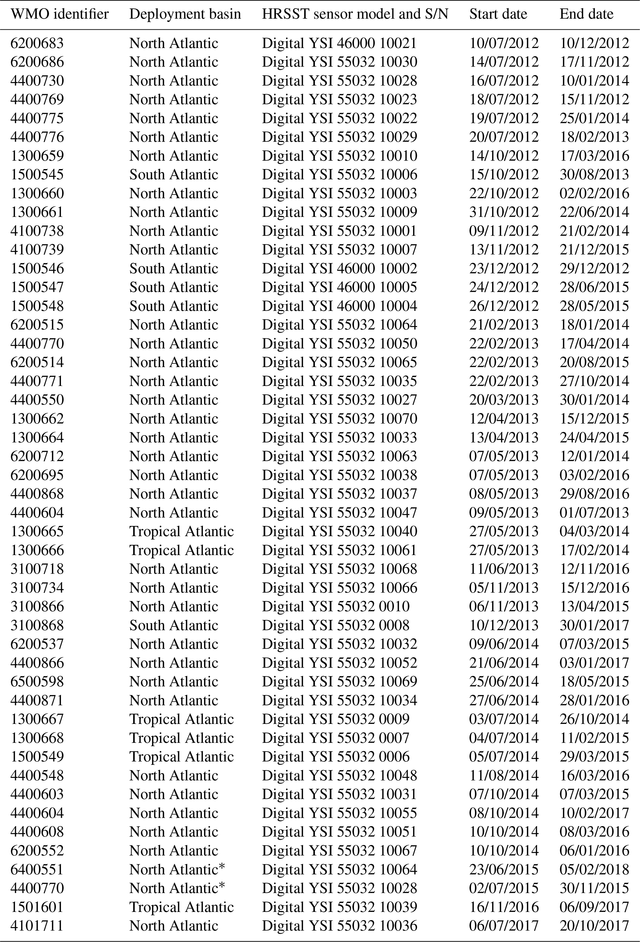
The fourth technical improvement was for each buoy to use an individually calibrated temperature probe, instead of one picked from a batch calibration, in order to guarantee the more stringent total uncertainty requirement of 0.05 K, as well as traceability to national standards. This requirement (on top of previous ones) was called “HRSST-2”. In total, 46 such HRSST-2 buoys fitted with all three technical advances, as well as including each a barometer, were deployed between 2012 and 2017. These buoys are listed in Table 1 below. They were manufactured by Metocean (Petolas, 2016), using Yellow Springs Instrument Company (YSI Inc.) sensors described in the table. One buoy was redeployed after running ashore.
Table 1Mission report of HRSST-2 SVP-B buoys. An asterisk indicates redeployment (note the WMO identifier may have changed, possibly reusing a number previously assigned to an earlier buoy). The third column shows SST sensor references.
In addition, several other HRSST-2 buoys were manufactured for experimental purposes, also by Metocean. Each buoy carried a conductivity–temperature (CT) probe manufactured by Sea-Bird Electronics (SBE) in order to measure salinity. Each HRSST-2 SVP buoy with barometer and salinity (SVP-BS) hence included two individual-calibrated SST probes: one integrated with the buoy hull (around 17 cm depth), and one in the CT probe (around 45 cm depth). This twin-sensor configuration offered near-optimal horizontal and temporal co-location by virtue of the buoy design. The only major differences between the two sensors were the vertical positioning and the housing of the sensors (one digital SST sensor integral with the hull, the other CT sensor immersed entirely in water). In total, there were 19 such buoys deployed between 2012 and 2015 (one buoy was redeployed after beaching). Table 2 shows the list of such buoys, the deployment areas, and the mission dates. Most buoys were deployed in the North Atlantic.
Table 2Similar to Table 1 but for HRSST-2 SVP-BS buoys (each buoy was also fitted with a CT probe).

2.2 HRSST-2 SVP-BS data record revisited
In order to exploit the co-located information from two individually calibrated SST probes, the data record from the second set of HRSST-2 buoys, SVP-BS fitted with CT probes, is addressed here. The record consists of about 87 000 data reports between 2012 and 2016. Figure 1 shows a scatter density plot of the two temperatures. The twin measurements are highly correlated, and the robust standard deviation of the difference is 0.03 K. This result is compatible with uncertainty in a difference of two sensors with total uncertainties better than 0.05 K (or possibly 0.02 K). However, Fig. 1 shows a small fraction of outliers in both directions, especially for warmer temperatures. In fact, the root mean square (rms) of the differences is quite large, at 0.36 K.
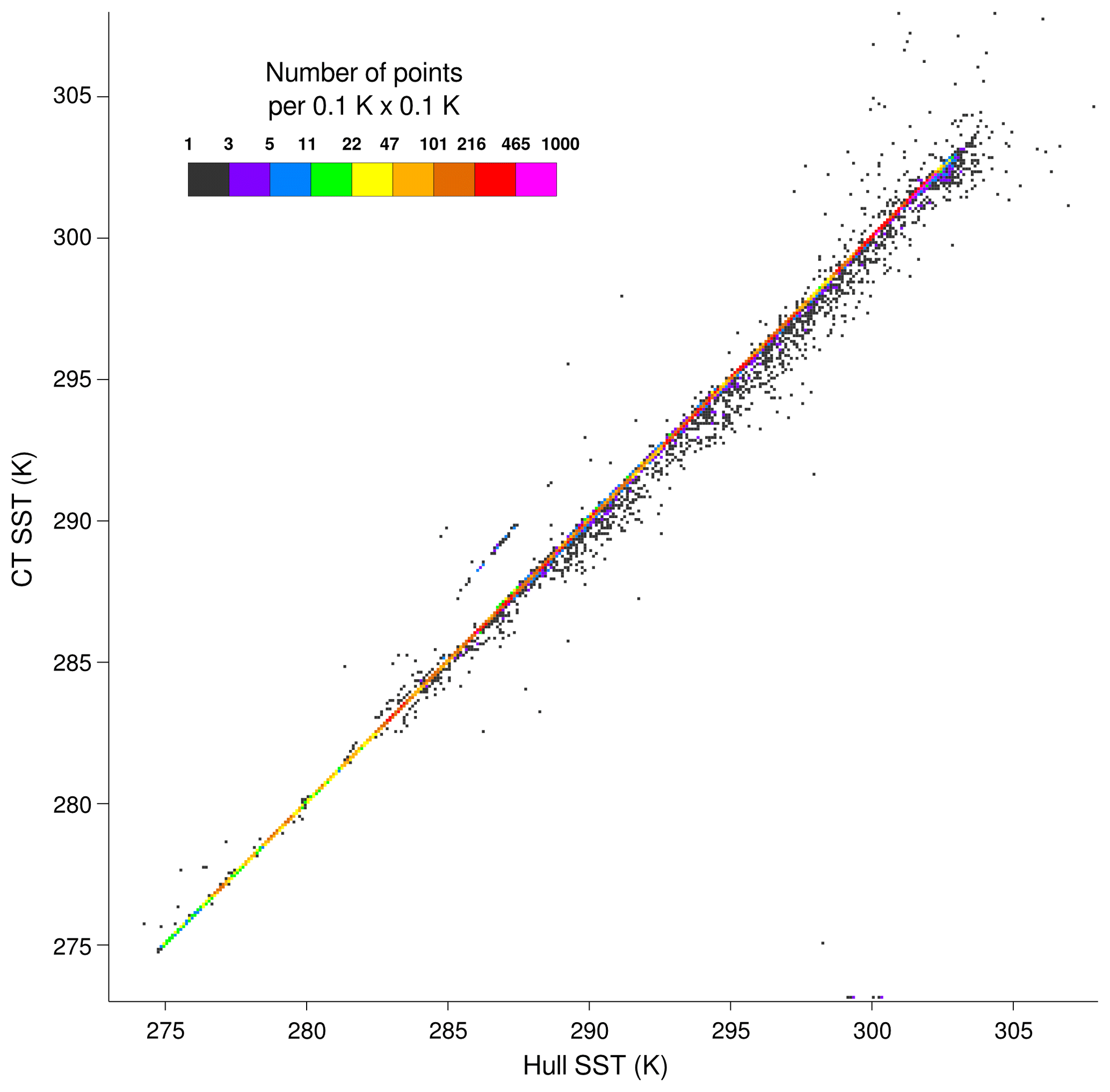
Figure 1Density plot of the scatter between hull SST measurements (horizontal axis) and CT SST measurements (vertical axis) from HRSST-2 SVP-BS buoys.
The differences between the two measurements are not only due to sensor accuracy but also to the placement of the sensors: vertical location and housing (one integral with the buoy hull, the other underneath the buoy). To better understand the sources of differences, Fig. 2a shows the differences between the two sensor temperatures as a function of solar elevation angle. Differences that are out of range (below −1 K or above 1 K) are also shown for completeness (at −1 and +1 K, respectively); they represent about 0.5 % of the entire data record. We find, as expected, that most large-magnitude differences (absolute value greater than 0.2 K) are positive during daytime (the hull sensor being located closer to the surface). The differences are smaller at night and when the Sun is more than 30∘ below the horizon. The large departures observed sometimes during daytime suggest that one or other of the two SST sensors may have been differentially affected by direct solar radiation, or by the buoy heating up the sensor through heat conduction.
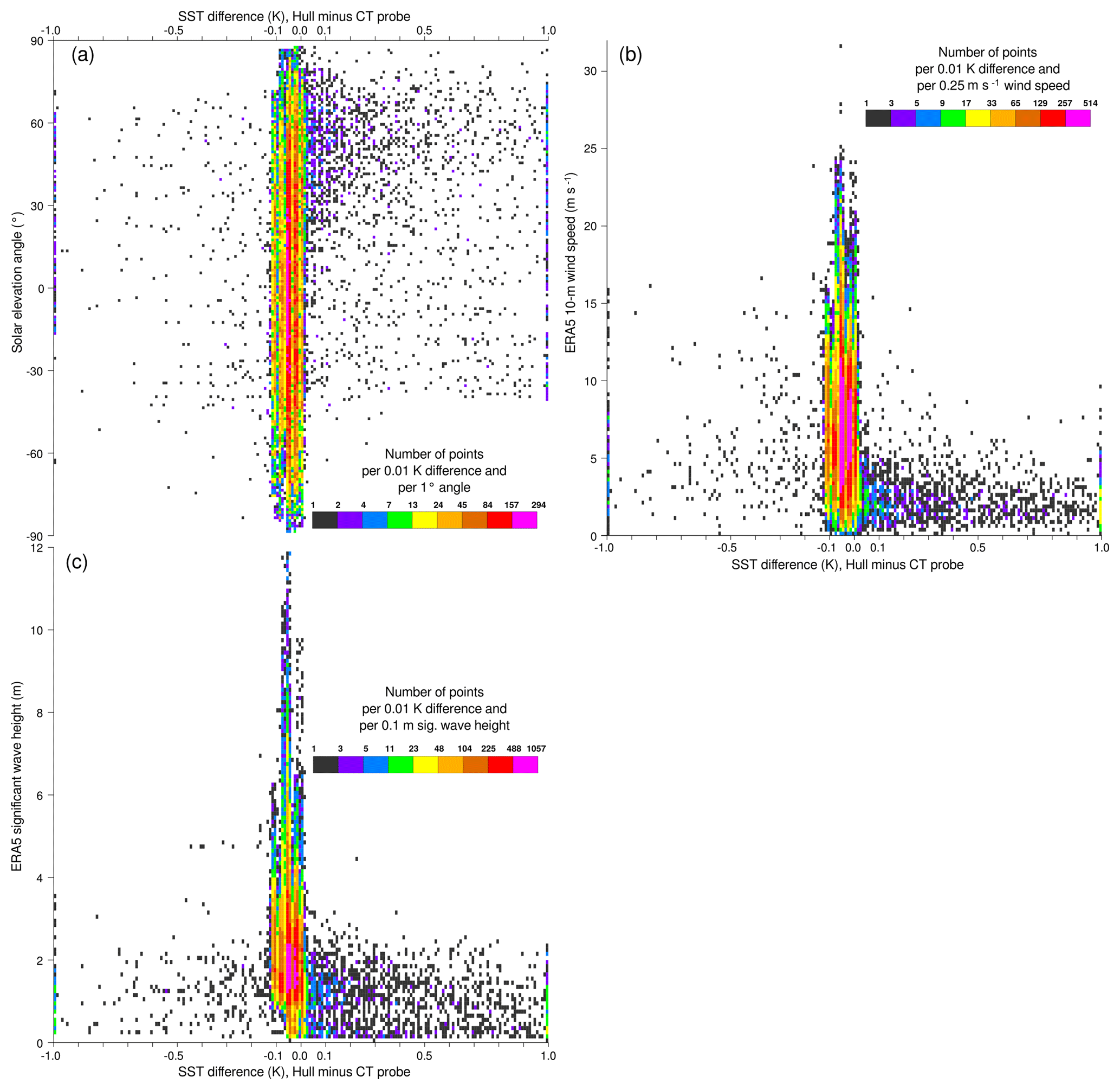
Figure 2Differences between the two SST sensors from all HRSST-2 SVP-BS buoys, as a function of (a) solar elevation angle and ERA5 estimates for (b) 10 m wind speed and (c) significant wave height.
Unlike promising new developments with wave drifters (Centurioni et al., 2016), the HRSST-2 drifters did not provide any information about sea state. In past SST studies, wind speed is generally used to describe sea-state mixing (e.g., Donlon et al., 2002; Morak-Bozzo et al., 2016). In this study, we also consider significant wave height. Information about both parameters can be obtained by co-locating with the ERA5 reanalysis (Hersbach and Dee, 2016; C3S, 2017). The ERA5 reanalysis data are interpolated in space from their original resolution (spectral truncation T639) to the buoy locations, using the nearest-in-time hourly reanalysis map. Figure 2b and c show (respectively) that the large-magnitude SST difference mostly arise when the wind speed is up to moderate (under 8–10 m s−1) and when the wave heights are up to moderate (under 2–3 m). The agreement between the sensors increases when there is more wave activity, probably because of greater mixing. When such is the case, almost all SST differences are found in the range from −0.1 to 0.0 K. Sea-state mixing caused by waves cannot be controlled or mitigated by a platform as small as a 40 cm diameter drifter. However, the role of the waves, probably via mixing, is suggested here to be quite important when using the SST data collected by drifting buoys. A knowledge of the local SST dynamics, as the buoy is following a pendulum movement and senses the temperature surface at various depths within the top few meters of the ocean, would help better understand the distribution of SST that is measured, and how it corresponds to satellite measurements, or how it should be considered in the cal/val process.
The differences between the probes can also be inspected as a function of mean solar local time (MSLT) for each buoy. For this, we only retain the buoys that reported at least for 250 days, without issue. For the subsequent data analysis, we filter out 12 cases when differences are larger than 20 K (visible in Fig. 1), likely to be erroneous. Figure 3 shows that the mean differences feature a diurnal cycle, with the maximum positive differences around 12:00 MSLT. This is consistent with the depth difference of the two probes in the context of diurnal vertical stratification of the surface temperature. Diurnal stratification tends to peak around 14 h (e.g., Reverdin et al., 2013; Morak-Bozzo et al., 2016), and temperature stratification larger than 0.1 K within the upper 0.5 m would tend to occur only at the lowest wind speeds. However, this daily cycle in difference may also be partially explained by the hull sensor being heated by the surrounding buoy and/or by direct solar radiation (an effect which might tend to peak more around 12 h MSLT). These latter effects are not related to the environment and should be avoided.
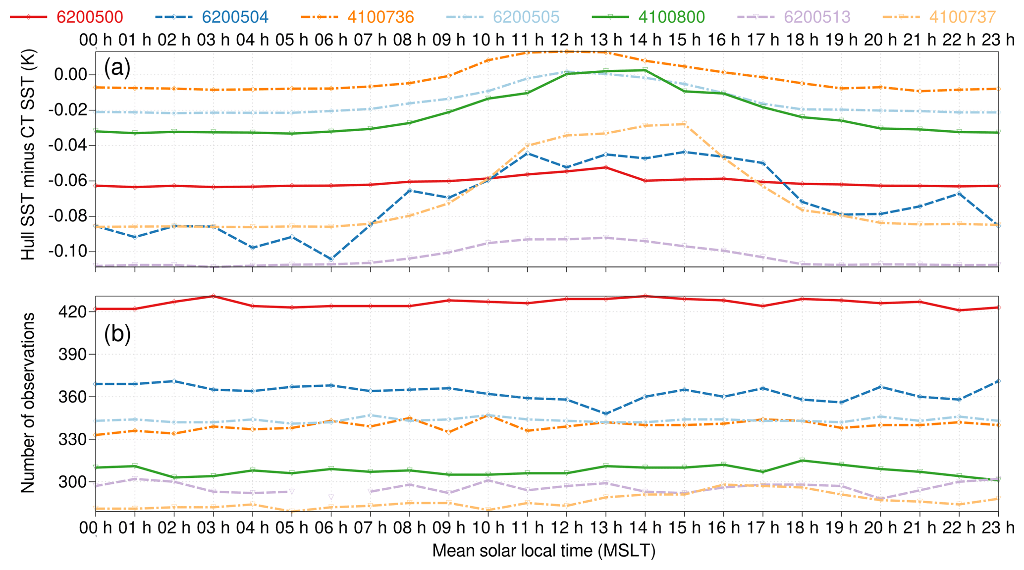
Figure 3Mean differences (a) between the two SST sensors, with the number of data records shown in panel (b), for HRSST-2 SVP-BS buoys that reported for at least 250 days (WMO identifier indicated in legend), as a function of mean solar local time (horizontal axis).
2.3 Recovered buoys
Three HRSST-2 buoys manufactured in 2012, deployed in 2014, ran ashore in 2016 in Great Britain and Brittany. They were recovered and offered together a unique opportunity to reassess sensor accuracy and drift several years after initial calibration. The buoys were recovered without visible outer damage. It is not impossible that the sensors may have aged differently during the various phases of the buoy life cycle: (a) after calibration and until deployment, (b) at sea, and (c) after recovery. Unfortunately, it proved impossible to have the probes calibrated by the same laboratory (Bernie Petolas, personal communication, 2016). Table 3 shows the results of the calibration verification done by the initial laboratory (Measurement Specialties, lab. no. 1 in the table), and the calibration verifications done by two other laboratories (at different dates), after the buoys were recovered from shore. Despite the same Metocean interface being used at all three laboratories, the calibration procedure, being inherently laboratory dependent, brings in additional uncertainties. For example, the various laboratories involved here did not use the same verification points. The initial laboratory used three calibration points (0, 25, 40 ∘C), i.e., the bare minimum to compute the three Steinhart–Hart coefficients per sensor. The same temperatures were then used to assess the (residual) calibration error. In the table, lab. no. 2 refers to the Service Hydrographique et Océanographique de la Marine (SHOM) metrology lab, which used seven verifications points (between 2 and 32 ∘C, at steps of 5 ∘C), and lab. no. 3 refers to the Scottish Association for Marine Science (SAMS) metrology lab, which used three verification points (0, 10, and 20 ∘C).
Table 3Individual calibration data for SST sensors from three HRSST-2 buoys that were fortuitously recovered. The mean error is the average difference, for several verification points, between the temperature reported by the sensor and the temperature of the calibration bath. Lab. no. 1 indicates the initial calibration and verification that was made then. The last column, showing temporal drift (in K year−1), is 365.25 times the difference between the mean error assessed by lab. no. 2 (or 3) minus the mean error assessed by lab. no. 1, divided by the number of days elapsed.
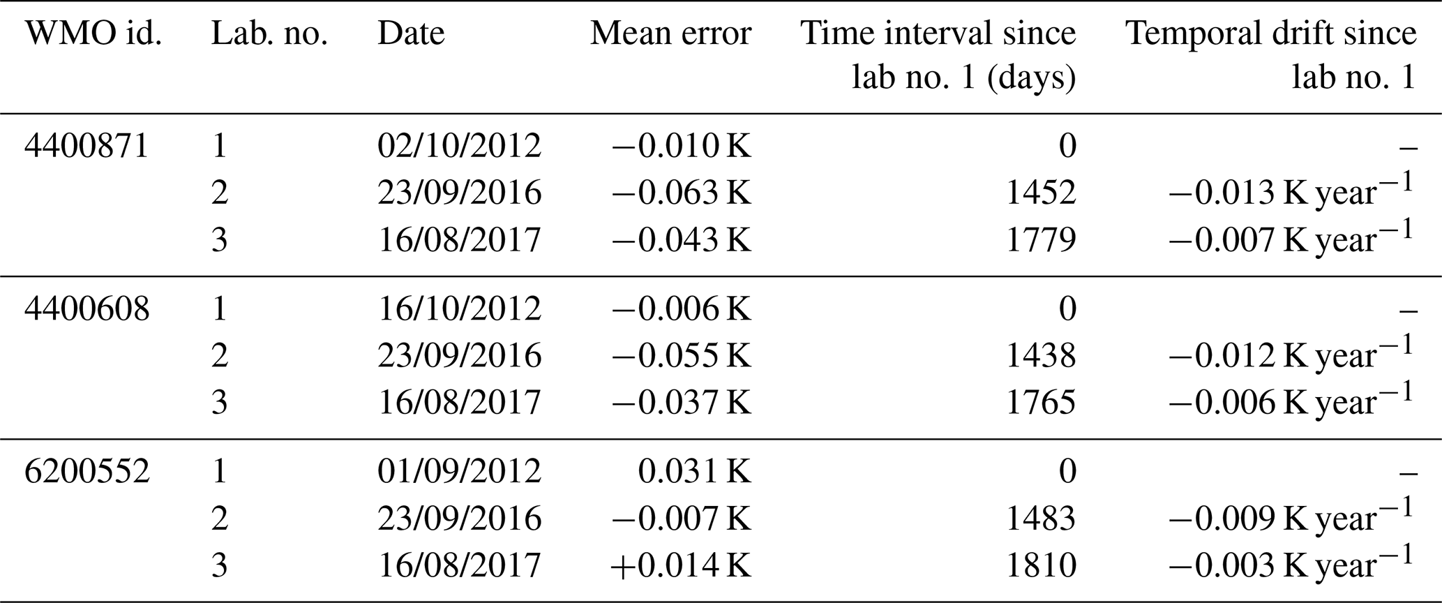
To remove the impact of different dates, the last column shows the estimated temporal drifts. The drift results vary in magnitude between the probes and the laboratories. This is probably mainly because of different choices for the verification temperatures, though other factors may have also played a role, such as probe resolution, probe response time, and temperature laboratory influence on the measurements (with the electronics not immersed in water), among others. However, all the results found here suggest negative trends, around −0.01 K year−1 for lab. no. 2 and −0.005 K year−1 for lab. no. 3.
Note that it cannot be ruled out that the probes, once removed from the buoys, did respond differently than during the initial calibration setup. Indeed, the temperature variations being looked at are very small, and any influence of the acquisition electronics may affect the results. The exact environment used for housing the electronics during calibration of the initial probes, as well as during the verifications, even if specified in the initial calibration sheets, cannot be replicated with certainty.
Consequently, these results are to be taken with caution, and the importance of the calibration apparatus stands out as being an important part of the traceability. However, should the negative trend (cooling) be confirmed, it would have an impact on the exploitation of the SST drifter data for satellite cal/val, as well as corrections that are made to global datasets. Recent adjustments have actually recognized buoys as being cooler than ships in terms of SST (Huang et al., 2015), in line with earlier findings (e.g., Emery et al., 2001; Rayner et al., 2010), though no difference was made especially for drifting buoys as a function of their “age”. The three recovered buoys achieved lifetimes of (respectively) 580, 515, and 453 days (see Table 1). These durations are close to or above the average drifter lifetime of 450 days (Lumpkin et al., 2012). Considering all the estimated temporal drifts shown in Table 3, the temperature biases of these drifters (averaged over the mission duration) would range between −0.002 and −0.010 K.
In conclusion, given the importance of drifting buoy SST in climate studies, the impossibility of putting together firm metrology results indicates that a better-documented calibration protocol is needed for the measurement of SST by these platforms, both to ensure initial calibration and calibration verification several years afterwards.
2.4 Evaluation of HRSST-1 and HRSST-2 drifters
The analysis of O'Carroll et al. (2008) identified the standard deviation of error of the drifting buoy network to be 0.23 K. An interpretation of this finding is it is equivalent to the standard uncertainty of the error distribution. An alternate approach to the method of O'Carroll et al. (2008) is to derive a theoretical uncertainty estimate for the satellite SST (Bulgin et al., 2016), which can then be validated using satellite/drifter differences (Lean and Saunders, 2013; Bulgin et al., 2016; Neilsen-Englyst et al., 2018). The concept of uncertainty validation is presented in detail by Corlett et al. (2014). Briefly, the standard deviation of the satellite/drifter differences is comprised of contributions from the satellite and drifter measurements, as well as terms to represent the spatial and temporal differences between the two measurements. Having used models to adjust the drifter measurement to be the same time and depth as the satellite SST, Corlett et al. (2014) showed the standard deviation of the satellite/drifter differences approximately reduces to two terms: the satellite SST uncertainty and the drifter SST uncertainty as in Eq. (1).
Figure 4 shows a comparison between 1 October 2016 and 30 June 2017 of satellite SST validation results for the dual-view three-channel retrieval from SLSTR for two sets of drifters: all drifters in Fig. 4a (15 551 matchups) and a subset of HRSST-1 and HRSST-2 drifters in Fig. 4b (625 matchups). In the figure, the green lines indicate the theoretical dispersion of uncertainties using Eq. (1) and a value of 0.20 K for σdrifter (an assumption between those of O'Carroll et al., 2008 and Lean and Saunders, 2013). The blue lines indicate the calculated dispersion for each set of data and the red lines indicate the standard error. If the assumptions are correct, then the dispersion of the blue lines should track the spread of the green lines, which we see is the case in Fig. 4a (all drifters). Where the dispersion does not match the expected spread, the large standard errors imply a low number of satellite/drifter differences in those bins. For the subset of HRSST drifters, Fig. 4b shows that the dispersion underestimates the spread, even for low standard error cases, meaning one assumption is incorrect in this case.
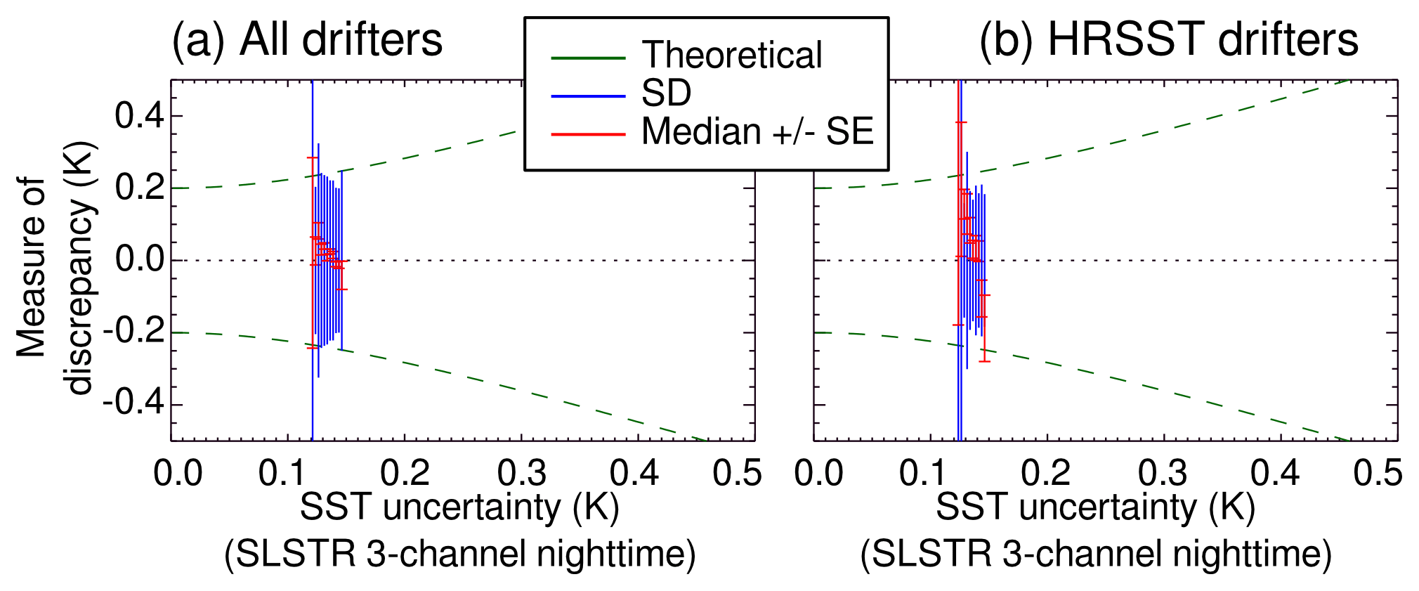
Figure 4SLSTR SST uncertainty validation plot for (a) all drifters and (b) a subset of HRSST-1 and HRSST-2 drifters, with uncertainty bins of 0.01 K. An uncertainty of 0.20 K is assumed for the drifter SST.
With all other factors being equal, the distinction in the drifter type between Fig. 4a and b suggests the drifter uncertainty assumed (0.20 K) is inappropriate for the HRSST subset. To verify this, Fig. 5 contains the same data as Fig. 4 but with the theoretical dispersion (green lines) calculated for a drifter uncertainty of 0.05 K. While the calculated dispersion does not track any more the expected spread for all drifters (Fig. 5a), the assumption of 0.05 K for the uncertainty of the HRSST drifter data gives a much better fit (Fig. 5b). This demonstrates the improved quality of HRSST drifter data for satellite SST validation.
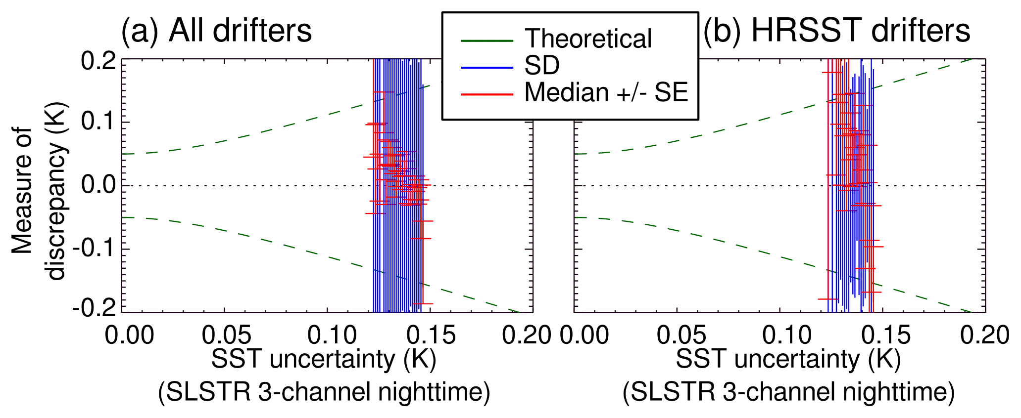
Figure 5SLSTR SST uncertainty validation plot for (a) all drifters and (b) a subset of HRSST-1 and HRSST-2 drifters, with uncertainty bins of 0.001 K. An uncertainty of 0.05 K is assumed for the drifter SST.
2.5 Influence of the drogue on drifter SST measurements
This section investigates the effect of the sea anchor or drogue on drifter SST measurements. By exerting its own weight and by following currents centered at 15 m depth, the drogue pulls the float downwards via the tether. This maintains the float and its drogue aligned in the vertical, in wave troughs. When the drogue is lost, the float has more freedom to oscillate by roll and pitch, and the temperature probe can sometimes be exposed to waters closer to the surface. Also, when in that situation, the float is more likely to reach wave crests. There, the sky visibility is improved, reducing the GPS time to first fix (TTFF), which can serve as an additional indicator of drogue loss (Petolas, 2013).
To investigate the influence of the drogue, the SVP-BS data record is revisited. These buoys used submergence sensors, whereas drifters nowadays use strain gauges, e.g., as indicated by Rio (2012), who developed a advanced method to identify drogue loss using drifter currents, satellite altimetry, and wind reanalysis data. The submergence (or tether strain gauge) readings are neither straightforward to interpret nor fully reliable on their own (Rio, 2012). However, the SVP-BS drifter data considered here (available from the Coriolis In Situ Thematic Assembly Center) are not found in the drifter dataset of Rio and Etienne (2018), which includes drogue presence flags. Consequently, for this analysis, we use the submergence and GPS TTFF data. A visual inspection indicates that 10 of the 20 buoys in Table 2 have lost their drogues during their mission. For these buoys, two series of data records are extracted: (1) before drogue loss and (2) after drogue loss.
During daytime, the median of the differences between the twin SST measurements is −0.04 K in (1), whereas it is −0.03 K in (2). The reduction in differences may appear insignificant, but it is consistent with the CT sensor being more often exposed to depths similar to the sensor integral to the hull when the drogue is lost than when the drogue is present. Similarly, the robust standard deviation of the differences between the twin SST measurements is 0.03 K in (1), whereas it is 0.01 K in (2). Again, this reduction is consistent with drogue loss for the same reasons.
During nighttime, no influence of the drogue loss is expected if the temperatures are homogeneous just below the surface. This is indeed what is observed. The median of the differences is −0.04 K in both (1) and (2), and the robust standard deviation of the differences is 0.03 K in both (1) and (2).
In other terms, the SVP-BS data record confirms the expectation that once the drogue is lost, the SST probes on a drifter are more likely to be exposed to water immediately below the surface than when the drogue is present, and this effect is more visible in the presence of stratification (e.g., during daytime). To keep track of the drogue effect on SST measurements, it is important to monitor drogue loss as well the immersion depth and its variations.
2.6 Limited traceability
Adopting a more general point of view for SST observations, several works have already attempted to document the uncertainties in the various in situ SST measurement methods. The present paper does not attempt to review all these efforts but cites relevant results from the comprehensive review of Kennedy (2014). While the focus of this earlier work was on the creation on long time series, with the largest issues identified at the time of World War II (transition on ships from bucket to engine-room intake), the quality of SST buoys was found to be the subject of several concerns. The first concern is the spread in quality between buoys, depending on the source of the uncertainty estimate, with no reliable link to the actual metrological reference. The second concern is a suggested improvement in quality over time, though without quantified evidence or clear a priori reason for it that would be explained by metrological documentation. Both points stem from an insufficient knowledge of the sensor technology, and of the calibration procedure that was actually used, for each drifting buoy deployed. The results shown earlier, showing differences in SST quality between general drifters versus HRSST drifters, reinforce the importance of enhancing the knowledge of drifter metrology and metadata.
The HRSST-2 efforts were initiated by the cal/val needs of AATSR SST retrievals. With the demise of this instrument after 10 years of service in 2012 (ESA Communications Department, 2012), the HRSST-2 developments were put to a halt, until the replacement sensor (SLSTR on Sentinel-3) was launched. However, this gap gave time to finish all HRSST-2 deployments and review the lessons learnt from them. Coupled with the need to assert long consistent time series of SST at an accuracy level compatible with SLSTR requirements, sound bases were used to imagine a novel sensor package for reference SST. The result is the SVP-BRST, based on the SVP-B design (Sybrandy et al., 2009), with a strain gauge to detect drogue loss. In addition, the HRSST-2 requirements presented earlier are included, as well as others, described hereafter.
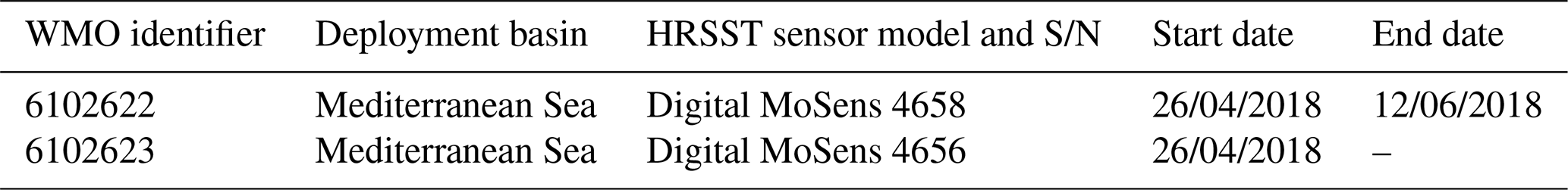
Table 4Similar to Table 1 but for two prototype SVP-BRST buoys (each buoy is fitted with a HRSST and static pressure probe).
The first additional requirement is to employ an additional HRSST sensor, in addition to the regular SST sensor. The HRSST sensor collects data within the 5 min before the round hour, when the position is updated by means of GNSS. The mean SST is to be computed from 1 Hz SST measurements. In addition, the data can be relayed at 1 Hz frequency for investigation. Furthermore, the distribution of SST observed within the 5 min is transmitted at coarse resolution (10th percentile, 30th percentile, 50th percentile or median, 70th percentile, and 90th percentile). This non-parametric information makes no assumption about the shape of the SST distribution: it can be used to drive an ensemble of applications, rather than using solely the mean SST, and to assess, for example, whether the SST distribution is symmetric.
Second, the HRSST sensor is removable from the buoy with simple tools (see Fig. 6), and includes a co-located pressure sensor that allows reporting static pressure with an accuracy of 5 cm in calm waters. Even if the instrument is affected by accelerations in wavy conditions, and the depth is only valid in rather calm conditions (when the sensor depth is already known by design), information can be derived about the hydrostatic water pressure variability (within 5 min).

Figure 6Sketch of the SVP-BRST (for the drogue, only the tether attachment is shown here), with the HRSST sensor unplugged shown in zoom panel (b). Note each SST sensor is protected from solar radiation by a cap.
Third, all SST sensors are insulated to shield them from unwanted effects caused by the non-water surrounding environment. This aims to avoid, for the SST sensors, exchanges by conduction with the buoy hull, exchanges by radiation with the Sun and the atmosphere, and radio interference from the buoy electronic board and antenna. This is done in practice by using, respectively, insulating material between the sensor and the buoy, a small cap to shield the SST sensor from radiation, and a metal plate underneath the buoy electronic board and antenna.
Fourth, the HRSST sensor is defined with a calibrating housing and protocol. Calibration coefficients are determined for each HRSST sensor individually so that their expanded calibration uncertainty can be assessed. These uncertainties are calculated according to the Guide For Uncertainty of Measurement (BIPM, 2008). They are found to be smaller than 0.01 K for each buoy. Response time and systematic errors related to the integration in the buoy have been assessed on two prototypes. The details of these laboratory measurements will be the subject of another paper.
Initial testing was conducted in the Brest area (see the Supplement). The results presented hereafter are based on data collected by the two prototypes in the Mediterranean Sea between 27 April and 11 June. The data are available in open access (see the section on data availability).
4.1 Deployment
Two SVP-BRST prototypes were deployed, as shown in Table 4. At the time of writing, the second prototype is still operating. Before deployment for release, the buoys were deployed briefly on 23 April for comparison in the seawater with an SBE-35 thermometer. The SST differences were then found to be −0.006 K for one buoy and −0.001 K for the other buoy, thereby meeting the 0.01 K claimed uncertainty. In comparison, the SST difference between the regular (or analogue) SST sensor with the SBE-35 was found to be −0.05 K (for both buoys).
4.2 Analysis of the data collected at sea
Once deployed on 26 April 2018, the buoys have followed the tracks shown in Fig. 7. The separation distance between the two buoys, initially under 1 km, remained under 10 km until 23 May. After that, the two buoys quickly diverged until the first one ran ashore.

Figure 7Trajectories of the two SVP-BRST prototypes after deployment on 26 April 2018. The two buoys separated on 22 May 2018. Map data: SIO, NOAA, US Navy, NGA, GEBCO; map image: Landsat/Copernicus.

Figure 8Time series of data collected by the two SVP-BRST prototypes until one of them ran ashore. Panels (a), (b), (e), and (f) also show, in lighter colors, ECMWF analyses co-located to the buoys dates, times, and locations.
The buoy reports data to shore using Iridium according to a binary data format number no. 091 documented by Blouch et al. (2018). Besides the usual parameters reported by SVP-B buoys (position, time, strain gauge, air pressure, analogue SST, and other technical parameters such as battery voltage and GNSS TTFF), one notes the following key additions: the mean temperature over 5 min reported by the HRSST sensor, 5 percentiles of the SST distribution within that time interval (10 %, 30 %, 50 % or median, 70 %, and 90 %), and the mean and the standard deviation of the hydrostatic water pressure during 5 min.
These parameters are shown in Fig. 8, where atmospheric pressure, SST, and significant wave height from the ECMWF operational analyses have been added. This information was co-located to the buoy dates, times, and locations using the same procedure as described in Sect. 2.2 (albeit at different horizontal and temporal resolutions). For the sake of comparing results, the time series are only for as long as both buoys were freely drifting (until 11 June).
The information from ECMWF analyses, although at a horizontal resolution of around 10 km, is independent from the buoys. It hence provides interesting information to consider when assessing the buoy data. For air pressure (Fig. 8a), both buoys agree with the ECMWF analyses to within 0.8 hPa rms. This is comparable to the state-of-the-art SVP-B deployed in this region.
For SST (Fig. 8b), the comparison to ECMWF analyses only suggests that the latter are typically lagging behind the buoy evolution by 24 h, until 5 June 2018. It must be remembered that the SST is not currently analyzed in the ECMWF prediction system, but this system was upgraded on 6 June, including a component to include atmosphere–ocean coupling (Buizza et al., 2018).
The depth inferred from the HRSST hydrostatic pressure sensor (Fig. 8c) shows values around 15 to 18 cm (which is the design location of the HRSST sensor). The spread between the two estimates is stable in time, around 4 cm. The calibration procedure of the pressure sensors may explain this difference. This remains however close to the design depth of 18 cm below the flotation line of the buoy.
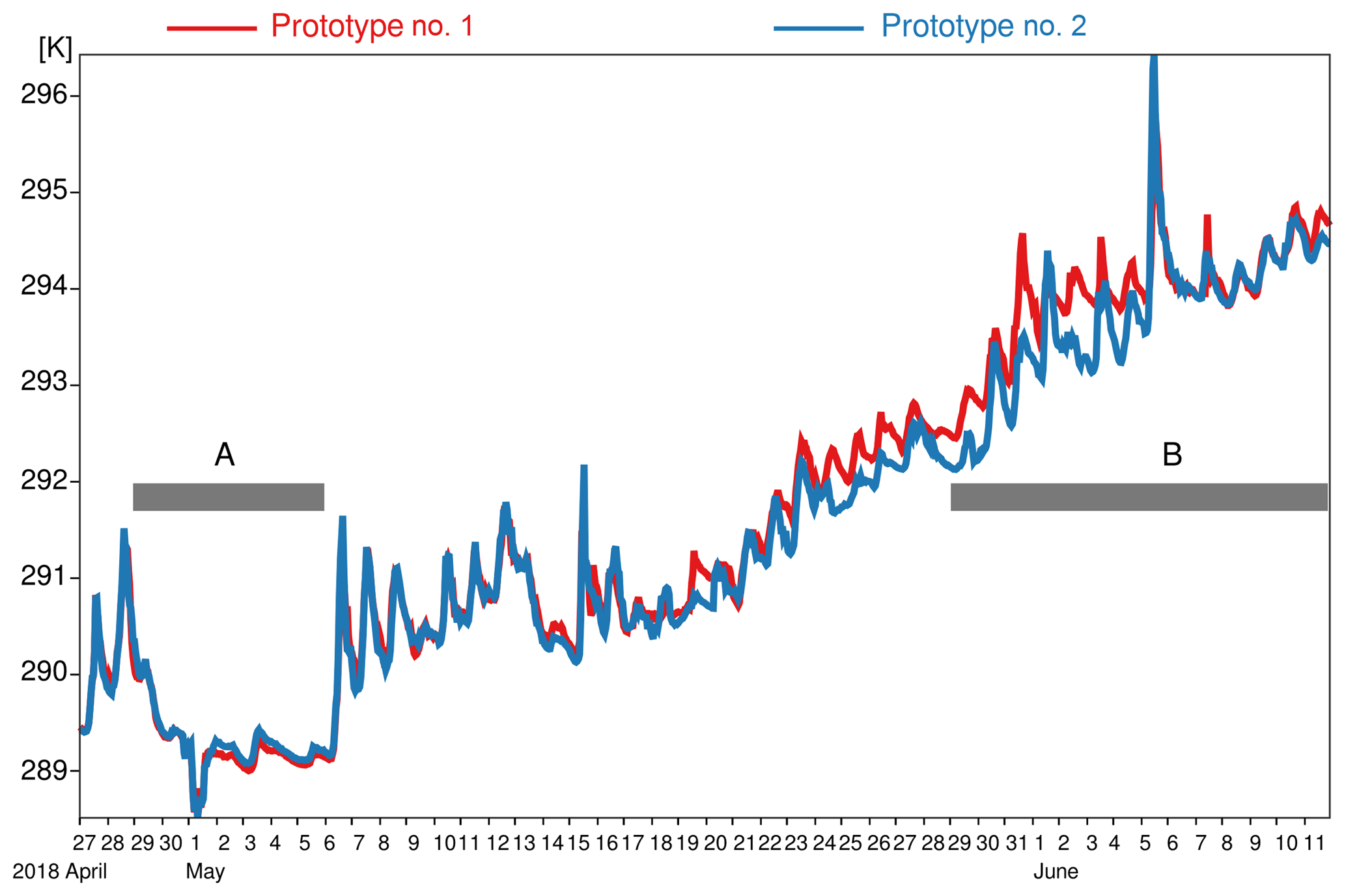
Figure 9Time series of the SST data, measured by the two SVP-BRST prototypes' HRSST sensors. A and B indicate two time periods selected for discussion.
The spread in the SST percentiles, shown in Fig. 8d, is usually within 0.1 K but sometimes exceed 0.3 K. In such situations, the calibration accuracy of the sensor is not of much help to help exploit the data for precise comparison with other sources. However, the availability of five estimates of SST, instead of just the mean, should help users move their applications to a small (five-member) ensemble and better understand how the spread in input in situ SST impacts their products.
Figure 8e shows the standard deviation of depth (inferred assuming hydrostatic equilibrium). This estimate varies between 1.5 and 3.5 cm. It is largest when the significant wave height (estimated by the ECMWF analyses) is largest, in line with stronger winds at the same times (Fig. 8f). This is expected from the buoy dynamics (as the pressure measured will be affected by positive and negative accelerations), and confirms that the ECMWF wind and wave height analysis appears to be correct. Given this result, the larger spread in SST percentiles appears to be well correlated with situations where the wave heights and wind speeds are smaller. This would seem to validate the conjectures formed earlier by revisiting the HRSST-2 SVP-BS data record, namely that the sea state is an important parameter to consider when exploiting the in situ SST data.
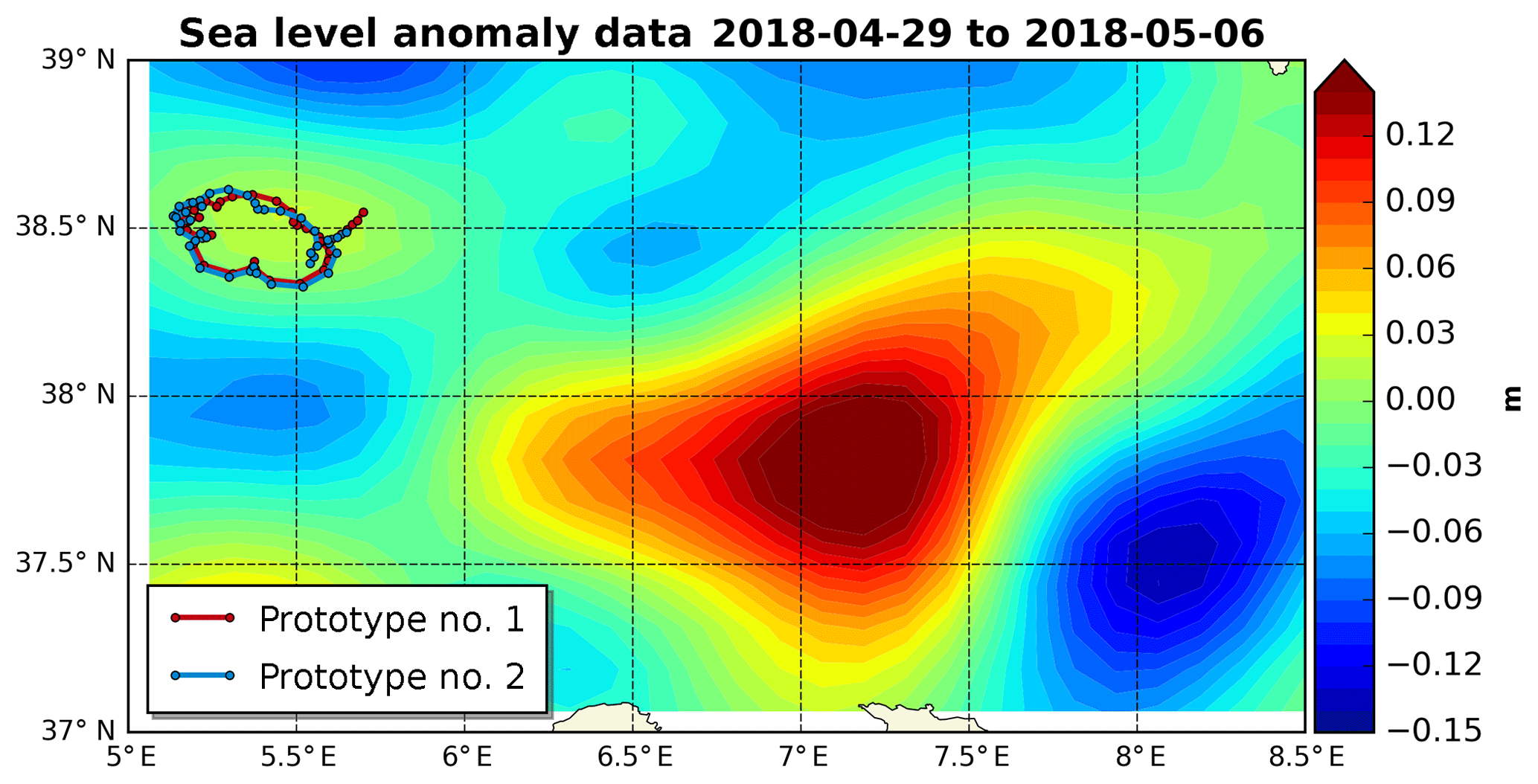
Figure 10Mean sea level anomaly map with the two SVP-BRST prototypes' tracks overlaid (prototype no. 1 in red, prototype no. 2 in blue) for the time period 29 April to 6 May 2018.
Regarding the SST data, we see that both buoys capture fairly well the diurnal warming/cooling cycle, a feature that is generally clearly missing from the ECMWF analyses. What is more, the amplitude of the daily cycle is variable, suggesting that the local ocean and atmospheric dynamics impacts the SST measured by the buoys. This is indeed the case for the period from 29 April to 5 May (time period A in Fig. 9): the observed SST is slightly cooler and, crucially, is missing the diurnal cycle found in the rest of the time series. Looking at co-located wind data (not shown), we do not find any clear modification, suggesting that the reason for this behavior in the SST data is principally oceanic and not atmospheric. Indeed, if we look at the buoys' location during that time period, we see that they are trapped within an eddy core (Fig. 10), and, significantly, it is a cold eddy. It is known that these eddies generate an upwelling within their core, leading to colder and vertically more homogeneous surface and near surface waters. The buoy data suggest that this upwelling more than compensates the diurnal warming and eliminates the near surface stratification. During time period A, the average diurnal cycle measured by the two buoys is rather weak (Fig. 11a and b).
Once the buoys move out of the eddy core (Fig. 12), the diurnal cycle is once again found in the data. This is visible in Fig. 9 during time period B, and in Fig. 11c and d, where the daily amplitude in SST exceeds 0.5 K (when it was less than 0.2 K in time period A).
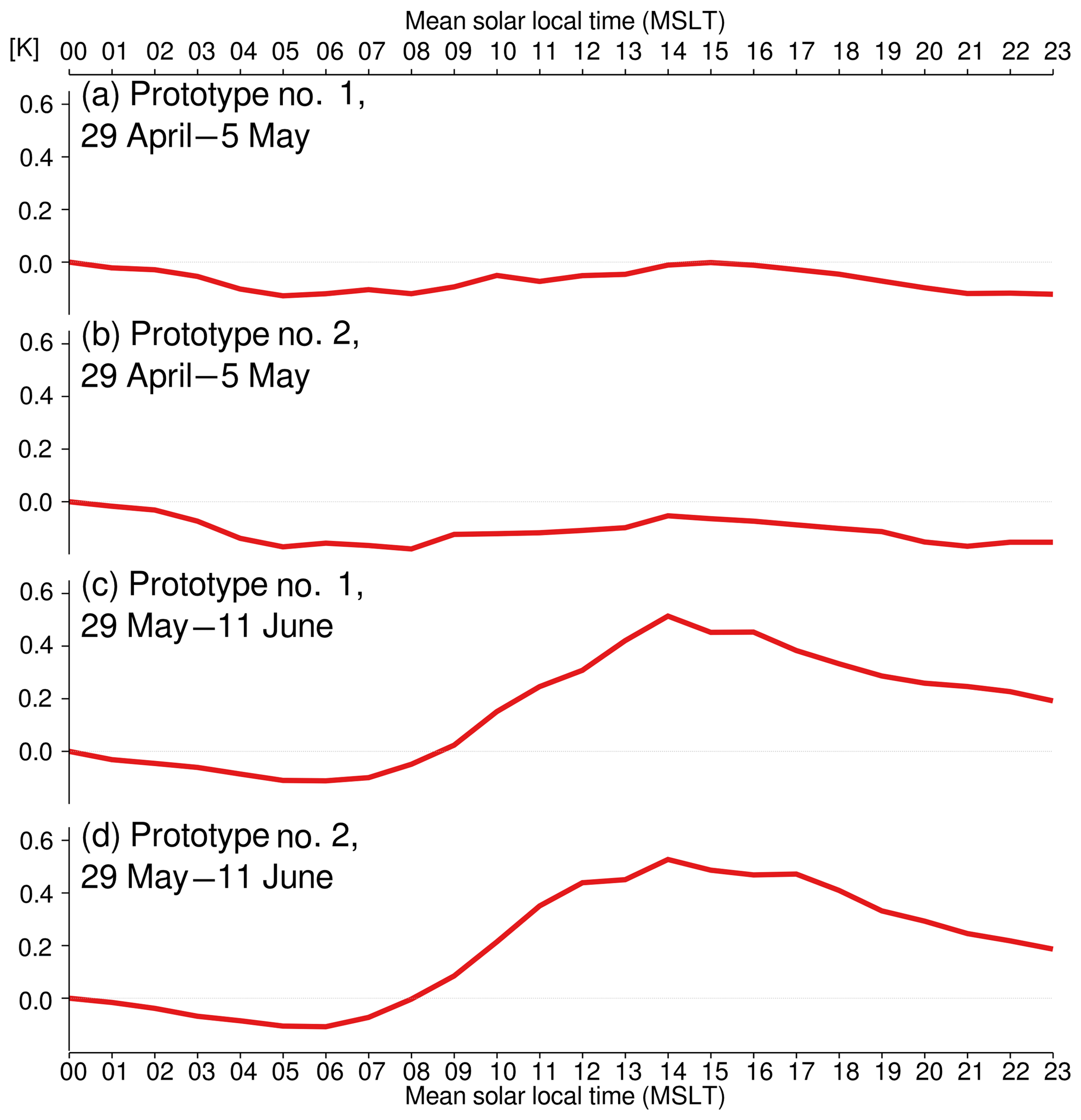
Figure 11Average SST diurnal cycle observed by the two SVP-BRST prototypes' HRSST sensors, during time periods A and B defined in Fig. 9. For each panel, the reference is the mean SST at 00:00 UTC. Horizontal thin dotted lines indicate zero.
Looking at the evolution of SST 5 min percentiles enables to gauge the small-scale variations in temperature near the surface. Figure 13 shows that the two buoys during time period A, as well as the first buoy during time period B, present smaller departures from the mean throughout the day than the second buoy during time period B. The maps in Figs. 10 and 12 may hold the clue to explaining this: in the first three cases, the buoys are the closest to eddies, while the fourth situation is when the buoy is traveling furthest from an eddy core. Overall, these remarks suggest that the ocean surface circulation may be of importance too, in addition to sea state, to properly exploit the in situ SST data for satellite cal/val, as this may affect the representativeness of the SST observed in situ.
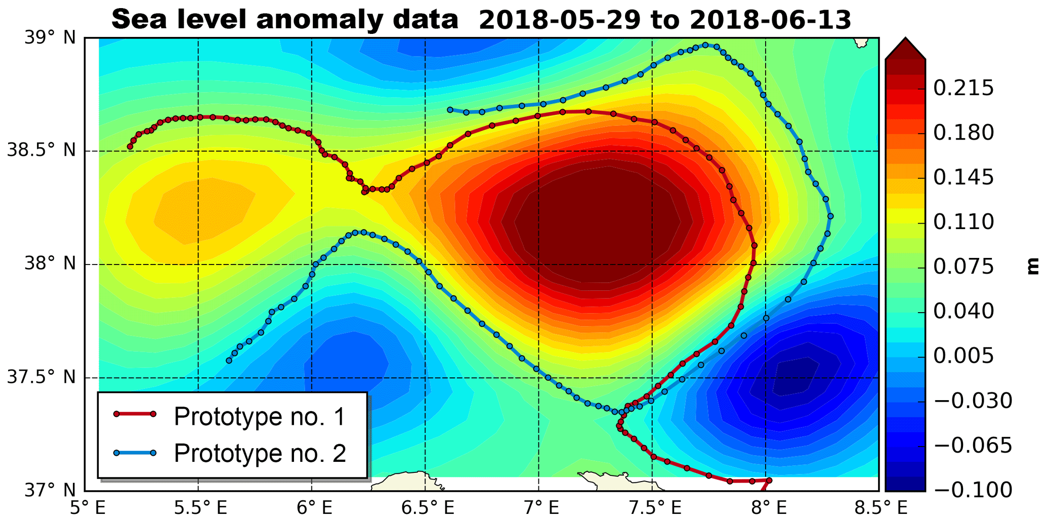
Figure 12Mean sea level anomaly map with the two SVP-BRST prototypes' tracks overlaid (prototype no. 1 in red; prototype no. 2 in blue) for the time period 29 May to 13 June 2018.
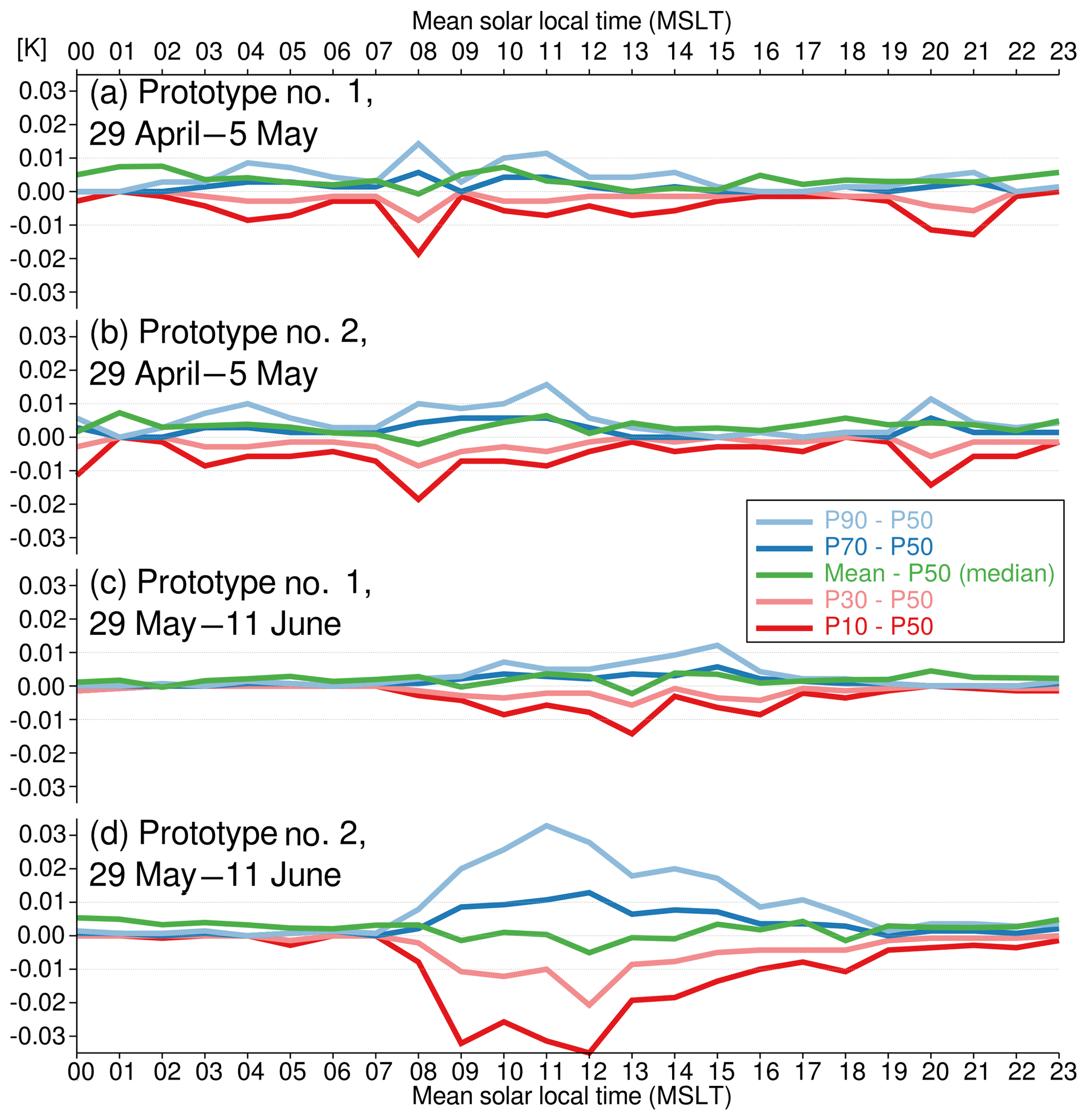
Figure 13Diurnal cycle of differences between each 5 min percentile (five percentiles are reported by the SVP-BRST prototypes: 10 %, 30 %, 50 % or median, 70 %, and 90 %), and the 5 min mean. Horizontal thin dotted lines indicate zero and ±0.01 K.
Revisiting the previous HRSST drifter initiatives, it was found that higher-quality SST was likely to be collected by such drifting buoys, as compared to general drifters. The following points were also identified to require further consideration, to improve upon HRSST-2 drifters. First, the sea-state dynamics, affected by the wind and wave activity, has influence on the vertical stratification, consistent with earlier findings (e.g., Dong et al., 2017), so the depth of the sensors is an important parameter to monitor. Second, the housing of the HRSST sensors needs to be insulated from external influences other than exchanges of heat with the seawater, in order to yield data that reflect the diurnal cycle without the effect of heat conduction from the buoy and heating of the sensor by direct solar radiation. Third, a better-documented protocol is needed for initial sensor calibration, allowing post-mission recalibration, to avoid introducing additional uncertainty through the use of unspecified calibration procedures. Fourth, traceability to national metrological standards needs to be established.
These findings were taken on-board to design a novel sensor package for SVP-B, for the sake of providing FRM SST data for the calibration and validation of satellite SST. The new buoy, called SVP-BRST, carries two SST sensors: one of standard manufacture, the other of absolute uncertainty better than 0.01 K (absolute uncertainty refers here to expanded uncertainty). In addition to measuring SST with improved calibration, the HRSST sensor also includes a hydrostatic water pressure sensor. The present paper indicates the initial design, which may evolve slightly as experience is gained from expected future deployments in greater numbers.
The two prototypes deployed in the Mediterranean Sea feature, before release, deviations within 0.01 K from a reference SBE-35 thermometer. Once freely drifting, the buoys observe that the SST spread within 5 min is usually smaller than 0.1 K, especially when the sea state is well mixed and the buoys are within an eddy core. The availability of percentiles from the 5 min distribution of SST sampled at 1 Hz (by a sensor with a fast response time) should help users improve their data processing chain to move towards an ensemble approach. The results in this paper suggest that it is important to consider the sea-state mixing and the ocean surface circulation to understand the representativeness of the in situ SST data, as they both affect observed SST variations (within the day and within 5 min). Consequently, they may both be worth considering in the process of satellite SST cal/val.
In addition, a fairly standard analysis, where ocean dynamics behavior can be inferred from the buoy data, suggests that the high-resolution SST data hold a wealth of information. Properly analyzed and interpreted, these data can provide a useful insight of the dynamics of the sampled area, especially when the Supplement is brought into the picture to consider sea state and ocean surface circulation. Even more interesting may be to collect full samples of 1 Hz data, when possible, in addition to the summaries of the distribution with five percentiles. Such a high-frequency HRSST dataset (HFHRSST) may serve other applications beyond satellite SST ca/val, such as fine-scale model developments and enhanced understanding of SST variability.
Future efforts include evaluation of the HRSST sensor drift. This will be done by keeping one SVP-BRST buoy at post in a monitored environment, and by recovering as many SVP-BRST buoys as possible. The goal will be to assess whether the temporal stability of SST from drifting buoys is within ±0.01 K year−1 after manufacture. This is important for climate monitoring, as initial results from past HRSST-2 buoys, presented in this paper, suggest temporal drifts that are systematically negative and close to this figure, though the very small number of drifting buoys surveyed (three) is not significant enough to be conclusive. At least 100 SVP-BRST buoys are expected to be deployed in the next 3 years, with a view to cover a wide range of atmospheric and oceanographic conditions.
The HRSST-2 SVP-B and SVP-BS data are available from the Copernicus In Situ Thematic Assembly Center (http://marine.copernicus.eu/situ-thematic-centre-ins-tac/, Copernicus Marine Environment Monitoring Service, 2019). The SVP-BRST prototype drifter data used in this publication are available in open access: https://doi.org/10.5281/zenodo.1410401 (Poli et al., 2018). Reanalysis ERA5 data are available from the Copernicus Climate Change Service.
The supplement related to this article is available online at: https://doi.org/10.5194/os-15-199-2019-supplement.
PP drafted the main text of this paper, prepared several of the figures and corresponding scientific analysis, and prepared the manuscript for submission. ML drafted the introduction and, along with GC, contributed results and scientific analysis. AD and MLM contributed to the buoy design and calibration. PB, DM, AO'C, KH, and CM contributed to the buoy design and scientific analysis.
Paul Poli, Marc Lucas, Anne O'Carroll, Marc Le Menn, Arnaud David, Gary K. Corlett, Pierre Blouch, Mathieu Belbeoch, and Kai Herklotz are participants in the TRUSTED project (see acknowledgements), which funds the development of the SVP-BRST buoy, as well as manufacturing of a series of units, deployments, and data and metadata acquisition and processing. David Meldrum and Christopher J. Merchant declare no conflict of interest.
The authors are funded by their respective institutions. Additional support,
including the development of the SVP-BRST prototypes and the resulting data
analyses, is provided by the European Union's Copernicus program for
funding the development of the SVP-BRST drifting buoys under the project
“Towards Fiducial Reference Measurements from HRSST drifting buoys for
Copernicus satellite validation” as part of the TRUSTED project led by CLS,
with buoy manufacturing by NKE, calibration by SHOM, coordination of
deployments by Météo-France, provision of a tethered reference measurement
by BSH, and metadata processing and deployment monitoring visualization
tools by JCOMMOPS. This publication contains modified Copernicus Climate
Change Service Information (2018) (C3S, 2017).
Edited by: Piers Chapman
Reviewed by: two anonymous referees
BIPM: Evaluation of measurement data – Guide to the expression of uncertainty in measurement, JCGM 100:2008, GUM 1995 with minor corrections, available at: https://www.bipm.org/utils/common/documents/jcgm/JCGM_100_2008_E.pdf, last access: 4 July 2018.
Blouch, P., Billon, C., and Poli, P.: Recommended Iridium SBD dataformats for buoys, v1.7, https://doi.org/10.5281/zenodo.1305120, 2018.
Bonekamp, H., Montagner, F., Santacesaria, V., Nogueira Loddo, C., Wannop, S., Tomazic, I., O'Carroll, A., Kwiatkowska, E., Scharroo, R., and Wilson, H.: Core operational Sentinel-3 marine data product services as part of the Copernicus Space Component, Ocean Sci., 12, 787–795, https://doi.org/10.5194/os-12-787-2016, 2016.
Buizza, R., Balsamo, G., and Haiden, T.: IFS upgrade brings more seamless coupled forecasts, ECMWF Newsletter, 156, Summer 2018, 18—22, available at: https://www.ecmwf.int/sites/default/files/elibrary/2018/18491-newsletter-no-156-summer-2018.pdf, last access: 31 August 2018.
Bulgin, C. E., Embury, O., Corlett, G., and Merchant, C. J.: Independent uncertainty estimates for coefficient based sea surface temperature retrieval from the Along-Track Scanning Radiometer instruments, Remote Sens. Environ., 178, 213–222, https://doi.org/10.1016/j.rse.2016.02.022, 2016.
Centurioni, L., Braasch, L., Di Lauro, E., Contestabile, P., De Leo, F., Casotti, R., Franco, L., and Vicinanza, D.: A new strategic wave measurement station off Naples port main breakwater, Coast. Engineer. Proc., 35, p. waves.36, ISSN 2156-1028, https://doi.org/10.9753/icce.v35.waves.36, 2016.
Copernicus Climate Change Service (C3S): ERA5: Fifth generation of ECMWF atmospheric reanalyses of the global climate, Copernicus Climate Change Service Climate Data Store (CDS), available at: https://cds.climate.copernicus.eu/cdsapp (last access: 1 July 2019), 2017.
Copernicus Marine Environment Monitoring Service: In Situ Thematic Centre (INS TAC), available at: http://marine.copernicus.eu/about-us/about-producers/insitu-tac/, last access: last access: 21 February 2019.
Coppo, P., Mastrandrea, C., Stagi, M., Calamai, L., Barilli, M., and Nieke, J.: The sea and land surface temperature radiometer (SLSTR) detection assembly design and performance, Proc. SPIE 8889, Sensors, Systems, and Next-Generation Satellites XVII, 888914, https://doi.org/10.1117/12.2029432, 2013.
Corlett, G. K., Merchant, C. J., Minnett, P. J., and Donlon, C. J.: Chapter 6.2 Assessment of Long-Term Satellite Derived Sea Surface Temperature Records, edited by: Zibordi, G., Donlon, C. J., and Parr, A. C., Experimental Methods in the Physical Sciences, Academic Press, 47, 639–677, https://doi.org/10.1016/B978-0-12-417011-7.00021-0, 2014.
Dee, D. P., Balmaseda, M., Balsamo, G., Engelen, R., Simmons, A. J., and Thépaut, J.-N.: Toward a Consistent Reanalysis of the Climate System, Bull. Amer. Meteor. Soc., 95, 1235–1248, https://doi.org/10.1175/BAMS-D-13-00043.1, 2014.
Dong, S., Volkov, D., Goni, G., Lumpkin, R., and Foltz, G. R.: Near-surface salinity and temperature structure observed with dual-sensor drifters in the subtropical South Pacific, J. Geophys. Res.-Oceans, 122, 5952–5969, https://doi.org/10.1002/2017JC012894, 2017.
Donlon, C.: Letter to Data Buoy Cooperation Panel (DBCP) Chair, in DBCP-29 Doc. 10.6, available at: https://www.jcomm.info/components/com_oe/oe.php?task=download&id=4752&version=1.0&lang=1&format=1 (last access: 4 July 2018), 2009.
Donlon, C.: Sentinel-3 Mission Requirements Traceability Document (MRTD), European Space Agency (ESA), available at: https://sentinel.esa.int/documents/247904/1848151/Sentinel-3-Mission-Requirements-Traceability, (last access: 7 September 2018), 2011.
Donlon, C. J., Minnett, P. J., Gentemann, C., Nightingale, T. J., Barton, I. J., Ward, B., and Murray, M. J.: Toward improved validation of satellite sea surface skin temperature measurements for climate research, J. Climate, 15, 353–369, https://doi.org/10.1175/1520-0442(2002)015<0353:TIVOSS>2.0.CO;2, 2002.
Emery, W. J., Baldwin, D. J., Schlüssel, P., and Reynolds, R. W.: Accuracy of in situ sea surface temperatures used to calibrate infrared satellite measurements, J. Geophys. Res., 106, 2387–2405, https://doi.org/10.1029/2000JC000246, 2001.
ESA Communications Department: Programmes in progress, Status at August 2012, ESA Bulletin 151, 58–87, available at: https://esamultimedia.esa.int/multimedia/publications/ESA-Bulletin-151/ (last access: 7 September 2018), 2012.
Hersbach, H. and Dee, D. P.: ERA5 reanalysis is in production, ECMWF Newsletter, 147, Spring 2016, 7, available at: https://www.ecmwf.int/en/newsletter/147/news/era5-reanalysis-production (last access: 3 July 2018), 2016.
Huang, B., Banzon, V. F., Freeman, E., Lawrimore, J., Liu, W., Peterson, T. C., Smith, T. M., Thorne, P. W., Woodruff, S. D., and Zhang, H.: Extended Reconstructed Sea Surface Temperature Version 4 (ERSST.v4) Part I: Upgrades and Intercomparisons, J. Climate, 28, 911–930, https://doi.org/10.1175/JCLI-D-14-00006.1, 2015.
Kennedy, J. J.: A review of uncertainty in in situ measurements and datasets of sea surface temperature, Rev. Geophys., 52, 1–32, https://doi.org/10.1002/2013RG000434, 2014.
Lean, K. and Saunders, R. W.: Validation of the ATSR Reprocessing for Climate (ARC) Dataset Using Data from Drifting Buoys and a Three-Way Error Analysis, J. Climate, 26, 4758–4772, https://doi.org/10.1175/JCLI-D-12-00206.1, 2013.
Llewellyn-Jones, D. T., Edwards, M. C., Mutlow, C. T., Birks, A. R., Barton, I. J., and Tait, H.: AATSR: Global Change and Surface Temperature Measurements from ENVISAT, ESA Bulletin 106, 12, available at: http://www.esa.int/esapub/bulletin/bullet105/bul105_1.pdf (last access: 7 September 2018), 2001.
Lumpkin, R., Maximenko, N., and Pazos, M.: Evaluating where and why drifters die, J. Atmos. Ocean. Tech., 29, 300–308, https://doi.org/10.1175/JTECH-D-11-00100.1, 2012.
Merchant, C. J., Embury, O., Roberts-Jones, J., Fiedler, E., Bulgin, C. E., Corlett, G. K., Good, S., McLaren, A., Rayner, N., Morak-Bozzo, S., and Donlon, C.: Sea surface temperature datasets for climate applications from Phase 1 of the European Space Agency Climate Change Initiative (SST CCI), Geosci. Data J., 1, 179–191, https://doi.org/10.1002/gdj3.20, 2014.
Morak-Bozzo, S., Merchant, C. J., Kent, E. C., Berry, D. I., and Carella, G.: Climatological diurnal variability in sea surface temperature characterized from drifting buoy data, Geosci. Data J., 3, 20–28, https://doi.org/10.1002/gdj3.35, 2016.
Neilsen-Englyst, P., Høyer, J. L., Toudal Pedersen, L., Gentemann, C. L., Alerskans, E., Block, T., and Donlon, C.: Optimal Estimation of Sea Surface Temperature from AMSR-E, Remote Sens., 10, 229, https://doi.org/10.3390/rs10020229, 2018.
O'Carroll, A. G., Eyre, J. R., and Saunders, R. W.: Three-Way Error Analysis between AATSR, AMSR-E, and In Situ Sea Surface Temperature Observations, J. Atmos. Ocean. Tech., 25, 1197–1207, https://doi.org/10.1175/2007JTECHO542.1, 2008.
Petolas, B.: Status and Performance of MetOcean Iridium Drifting Buoys, DBCP-29 Sci. Tech. Workshop, available at: https://www.jcomm.info/index.php?option=com_oe&task=viewDocumentRecord&docID=11847 (last access: 27 November 2018), 2013.
Petolas, B.: The Metocean HRSST sensor and its implementation, GHRSST 2016 Workshop on Traceability of Drifter SST Measurements, 13–14 October 2016, Scripps Institution for Oceanography, La Jolla, CA, USA, available at: http://empir.npl.co.uk/frm4sts/wp-content/uploads/sites/3/2016/10/3-2-Petolas-Metocean-presentation-SST-workshop-October-2016.pdf (last access: 7 September 2018), 2016.
Poli, P., Lucas, M., O'Carroll, A., Le Menn, M., and David, A.: Preliminary data collected by 2 prototype Surface Velocity Platform drifters with Barometer and Reference Sensor for Temperature (SVP-BRST) [Data set], Zenodo, https://doi.org/10.5281/zenodo.1410402, 2018.
Rayner, N. A., Kaplan, A., Kent, E. C., Reynolds, R. W., Brohan, P., Casey, K. S., Kennedy, J. J., Woodruff, S. D., Smith, T. M., Donlon, C., Breivik, L.-A., Eastwood, S., Ishii, M., and Brandon, T.: Evaluating Climate Variability and Change from Modern and Historical SST Observations, in: Proceedings of OceanObs'09: Sustained Ocean Observations and Information for Society, edited by: Hall, J., Harrison, D. E., and Stammer, D., European Space Agency, 2, 819–829, 2010.
Reverdin, G., Morisset, S., Bellenger, H., Boutin, J., Martin, N., Blouch, P., Rolland, J., Gaillard, F., Bouruet-Aubertot, P., and Ward, B.: Near–Sea Surface Temperature Stratification from SVP Drifters, J. Atmos. Ocean. Tech., 30, 1867–1883, https://doi.org/10.1175/JTECH-D-12-00182.1, 2013.
Rio, M.: Use of Altimeter and Wind Data to Detect the Anomalous Loss of SVP-Type Drifter's Drogue, J. Atmos. Ocean. Tech., 29, 1663–1674, https://doi.org/10.1175/JTECH-D-12-00008.1, 2012.
Rio, M.-H. and Etienne, H.: Global Ocean delayed mode in-situ observations of ocean surface currents, SEANOE, https://doi.org/10.17882/41334, 2018.
Sybrandy, A. L., Niiler, P. P., Martin, C., Scuba, W., Charpentier, E., and Meldrum, D. T.: Global Drifter Programme Barometer Drifter Design Reference, DBCP Rep. 4, rev. 2.2, available at: http://www.jcommops.org/doc/DBCP/svpb_design_manual.pdf (last access: 3 July 2018), 2009.
Theocharous, E., Fox, N. P., Barker-Snook, I., Niclòs, R., Garcia Santos, V., Minnett, P.J., Göttsche, F. M., Poutier, L., Morgan, N., Nightingale, T., Wimmer, W., Høyer, J., Zhang, K., Yang, M., Guan, L., Arbelo, M., and Donlon, C. J.: The 2016 CEOS infrared radiometer comparison: Part 2: Laboratory comparison of radiation thermometers, J. Atmos. Ocean. Tech., https://doi.org/10.1175/JTECH-D-18-0032.1, 2019.