Commonly used methods fail to detect known propagation speeds of simulated signals from time–longitude (Hovmöller) diagrams

This work examines the accuracy and validity of two variants of Radon transform and two variants of the two-dimensional fast Fourier transform (2-D FFT) that have been previously used for estimating the propagation speed of oceanic signals such as sea surface height anomalies (SSHAs) derived from satellite-borne altimeters based on time–longitude (Hovmöller) diagrams. The examination employs numerically simulated signals made up of 20 or 50 modes where one, randomly selected, mode has a larger amplitude than the uniform amplitude of the other modes. Since the dominant input mode is known ab initio, we can clearly define “success” in detecting its phase/propagation speed. We show that all previously employed variants fail to detect the phase speed of the dominant input mode when its amplitude is smaller than 5 times the amplitude of the other modes and that they successfully detect the phase speed of the dominant input mode only when its amplitude is at least 10 times the amplitude of the other modes. This requirement is an unrealistic limitation on oceanic observations such as SSHA. In addition, three of the variant methods detect a dominant mode even when all modes have the exact same amplitude. The accuracy with which the four methods identify a dominant input mode decreases with the increase in the number of modes in the signal. Our findings are relevant to the reliability of phase speed estimates of SSHA observations and the reported “too fast” a phase speed of baroclinic Rossby waves in the ocean.

1 Introduction

Time–longitude (Hovmöller) diagrams at a given latitude of an oceanic variable, η(x, t), that represents, for example, temperature, sea surface height, chlorophyll, obtained for example by satellite observations are often used for estimating the propagation rate of the oceanic variable. The rate at which η(x, t) propagates is determined by the inverse slopes of same-amplitude contours. These slopes are calculated by applying various methods, employed in image processing and detailed below in Sect. 2.2, to the raw data or to processed data (e.g., Polito and Liu, 2003, who separated the data into tiles of different periods). The methods examined here were used in many oceanic sub-areas such as the propagation speed of Rossby waves using SSHA (e.g., Tulloch et al., 2009) or data other than SSHA (Belonenko et al., 2018; Xie et al., 2016); nearshore wave dynamics (Almar et al., 2014); eddy detection (Abernathey and Marshall, 2013; Oliveira and Polito, 2018) and intraseasonal variability from mooring (Hu et al., 2018) to name a few.

De-Leon and Paldor (2017a) examined the accuracy of various methods in estimating the phase speed of waves by applying these methods to an artificially generated signal made of three sine functions (modes) with known phase speeds and amplitudes, compounded by large-amplitude random white noise. All methods have successfully filtered out the high-amplitude white noise from the three-harmonic signal and accurately detected the main mode (some of them also detected the secondary modes). However, such a signal is too synthetic/ideal and cannot be compared to real oceanic observations that include tens, if not hundreds, of modes with different frequencies and propagation speeds and not just three modes compounded by white noise.

In this short study we simulate oceanic observations and examine whether the methods detect a single dominant propagation speed out of many (20 or 50) speeds. In Sect. 2 we provide details on the generation of “observed” (i.e., simulated) η signal, the methods for evaluating the propagation speed of the signal and the tests we apply to the signals. The results are shown in Sect. 3 and discussed in Sect. 4.

2 Data and methods

2.1 Generating the simulated observations

The η signals (where η is any oceanic variable) used here are generated numerically by summing up N purely propagating sine functions (modes, hereafter) of the form sin (kx−ωt), where k is the zonal wavenumber, x is longitude, t is time and ω=kC is the frequency (where C is the zonal propagation speed). The number of participating modes, N, is taken to be either 20 or 50, and N−1 of these modes have an amplitude of 1 while the amplitude of the additional Nth, randomly chosen, mode is either larger than or equal to 1. The sum of all N modes constitutes the η-signal which is analyzed by the methods described in Sect. 2.2.

The spatial domain (x) is chosen between longitudes 70 and 130^∘ on a Cartesian grid with a $\mathrm{1}/\mathrm{4}{}^{\circ }$ resolution, and the time (t) duration is 20 years (1044 weeks) with temporal resolution of one datum per week, similar to publicly distributed products by e.g., Aviso. The values of the propagation speeds, C, are uniformly distributed in the −18 to 0 cm s⁻¹ range (i.e., each of the 20 or 50 modes is assigned a different propagation speed within that range), which is typical for baroclinic Rossby waves in the ocean (see e.g., Fig. 7 of Killworth et al., 1997; Barron et al., 2009). The values of the frequencies, ω, are selected randomly so that the period, 2π∕ω, falls in the range between 5 and 200 weeks while the values of the zonal wavenumbers, k, equal ω∕C. The resulting signal was low-pass filtered by applying a 5-week running average at each grid point to eliminate short-term variations.

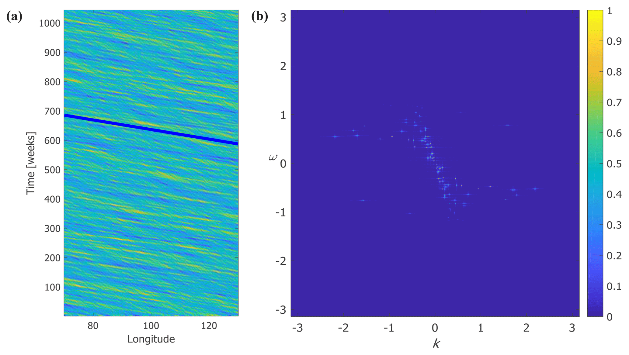
Figure 1 (a) An example of an artificial observed signal. (b) The associated (ω, k) diagram obtained by applying 2-D FFT to the signal of panel (a). The solid blue line in panel (a) corresponds to the randomly chosen dominant input mode's propagation speed.

The η signal made up of the filtered signal (i.e., the sum of N pure sine waves) at a given latitude is plotted as a function of longitude and time (Hovmöller diagram). When a single dominant mode exists that has a certain propagation speed the pattern on this diagram is a straight line whose slope is the inverse of the dominant propagation speed (since the abscissa is longitude and the ordinate is time). An example of a time–longitude diagram of an artificial signal is shown in Fig. 1a (for signal with dominant input mode's amplitude of 1.5) where the slope of the solid blue line corresponds to the propagation speed of the dominant input mode. The challenge is to estimate the dominant speeds using different methods and examine their success in detecting the propagation speed of the known dominant input mode. The methods examined here are detailed in the next subsection.

2.2 Methods for estimating the observed propagation speed

Four variants of methods have been employed for identifying the preferred direction of the same-amplitude contours on the Hovmöller diagram; each variant relates a certain measure of the power/intensity in a mode to its propagation speed. The first method is the Radon transform, used by e.g., Chelton and Schlax (1996), Chelton et al. (2003), and Tulloch et al. (2009) for analysing satellite observations of the ocean. In this method, one calculates the sum of the amplitudes along lines inclined at an angle θ and displaced a distance s from the origin. Then, the sum of squares of the values of these sums along all lines having the same angle is calculated. The angle at which this sum of squares is maximal is the best estimate for the orientation of the lines on the image. The dominant propagation speed of the signal is then proportional to the tangent of this angle of maximum sum of squares. In the second method, which is a variant of the Radon transform, the variance of the amplitudes is calculated along every angle θ instead of the sum of amplitudes. This method was applied e.g., by Polito and Liu (2003, to local auto-correlation of segments of Hovmöller diagram) and Barron et al. (2009). Another, independent, method commonly used (e.g., Zang and Wunsch, 1999; Osychny and Cornillon, 2004) is the 2-D fast Fourier transform (2-D FFT). An example of a (ω, k) diagram, obtained by applying 2-D FFT to the signal of Fig. 1a is shown in Fig. 1b. Here we use two variants of the 2-D FFT method: in the first variant one sweeps over the 2-D FFT spectra to find the direction in (ω, k) plane with maximum energy (this is the third method) while in the second variant one finds the maximal amplitude of the 2-D FFT (i.e., one of the bright points in Fig. 1b) and calculates the ratio ω∕k, where ω and k are the frequency and zonal wavenumber of the maximal amplitude (this is the fourth method). A detailed description of these methods and the interpretation of observed signals are found in De-Leon and Paldor (2017a).

Figure 2 An application of the four methods to the artificially generated signal shown in Fig. 1a (panel a: Radon transform, panel b: variance, panel c: 2-D FFT sweeping, panel d: 2-D FFT maximal amplitude). Blue lines correspond to the dominant input mode propagation speed and dashed black lines correspond to the input modes' propagation speeds.

Each of the four variants of the methods can yield an estimate of the dominant propagation speed of a signal, based on the extremum of a graph that relates the calculated measure of a mode's intensity to its propagation speed. An estimation of the propagation speed based on a local extremum of this graph is accepted when this extremum is narrow and isolated compared to other local extrema. When the normalized amplitude (the term normalized amplitudes is used for the calculated amplitudes divided by the maximal amplitude in the domain) of a distinct peak is 1 while the (normalized) amplitudes of all other peaks are smaller than (an arbitrarily determined value of) 0.8, this mode is considered the dominant mode. In the variance method, where the extrema are minima, the dominant mode is accepted when its normalized amplitude is 0.0 while the normalized amplitudes of all other minima are larger than 0.2. The results shown in Fig. 2 demonstrate that, in the particular signal of Fig. 1, in one method (2-D FFT maxima) no dominant peak exists (Fig. 2d) while in the other three methods dominant peaks exist, either a clear maximum (Fig. 2a, 2c) or a clear minimum (Fig. 2b), but they do not coincide with the dominant input mode (the blue line).

2.3 Examining the accuracy of dominant mode detection

Two types of tests are applied to these observations to examine the accuracy of the various methods in assessing the existence of a dominant propagation speed (i.e., mode) in the signal.

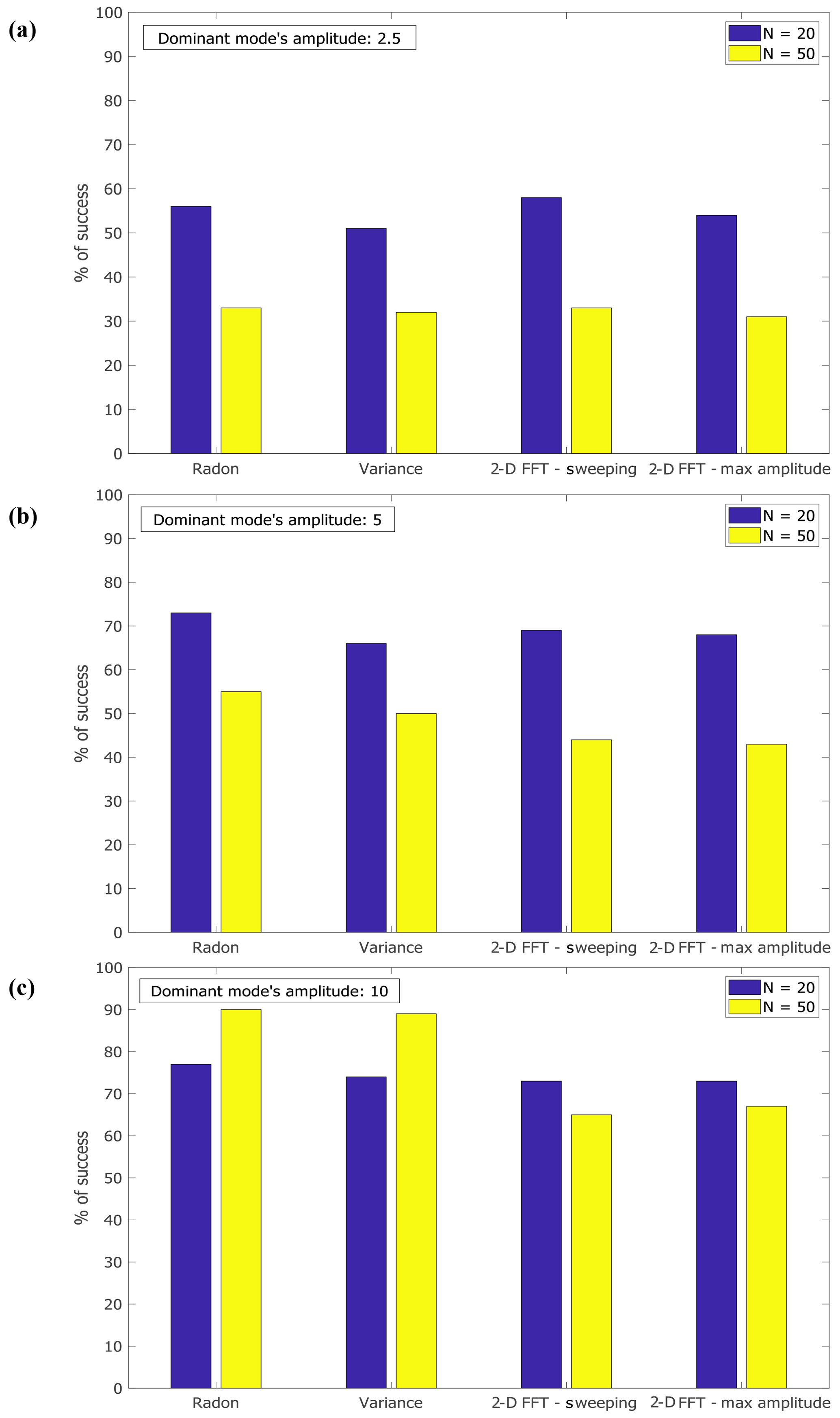
Figure 3 The percentage of success of each variant of the methods for dominant input mode's amplitude of 2.5 (a), 5 (b) and 10 (c) for both N=20 and N=50.

The first test is a true-positive/false-negative test in which there is a dominant mode in the observed signal, and a given method indicates whether this dominant mode exists (true-positive; TP) or not (false-negative; FN). In our case, one of the sine functions (this is the dominant input mode) is chosen randomly and its amplitude is set to be larger than 1. We check for each method if (at all) it identifies a dominant mode and if so, if it matches the propagation speed of this (larger amplitude) input mode. We divide the interval of propagation speeds into N (=20 or 50) bins of equidistant values, and the determination of the success of the methods in identifying a dominant mode is as follows: if the dominant mode found by the method falls in the expected bin of the dominant input mode, we assign a score of 1 (“TP”). If it is found in one of its next neighbours, it is assigned a score of 1∕2. A score of 0 (“FN”) is assigned when the method cannot find any dominant mode and when it detects a dominant mode more than one bin away from the correct bin. For each of five values of dominant mode's amplitudes: 1.5, 2, 2.5, 5 and 10 and for two values of N (20 or 50) we repeat this procedure 50 times (i.e., for 50 different signals), sum up the scores and calculate the percentage of success in identifying the dominant input mode in the signals by TP/(TP+FN)×100. Since this choice of scoring (1, 1∕2, 0) is arbitrary, we also considered an alternative arbitrary choice for scoring: 1 if the dominant mode falls in the expected bin of the dominant input mode, 2∕3 in one of its nearest neighbours, 1∕3 in one of its next to nearest neighbours and 0 otherwise.

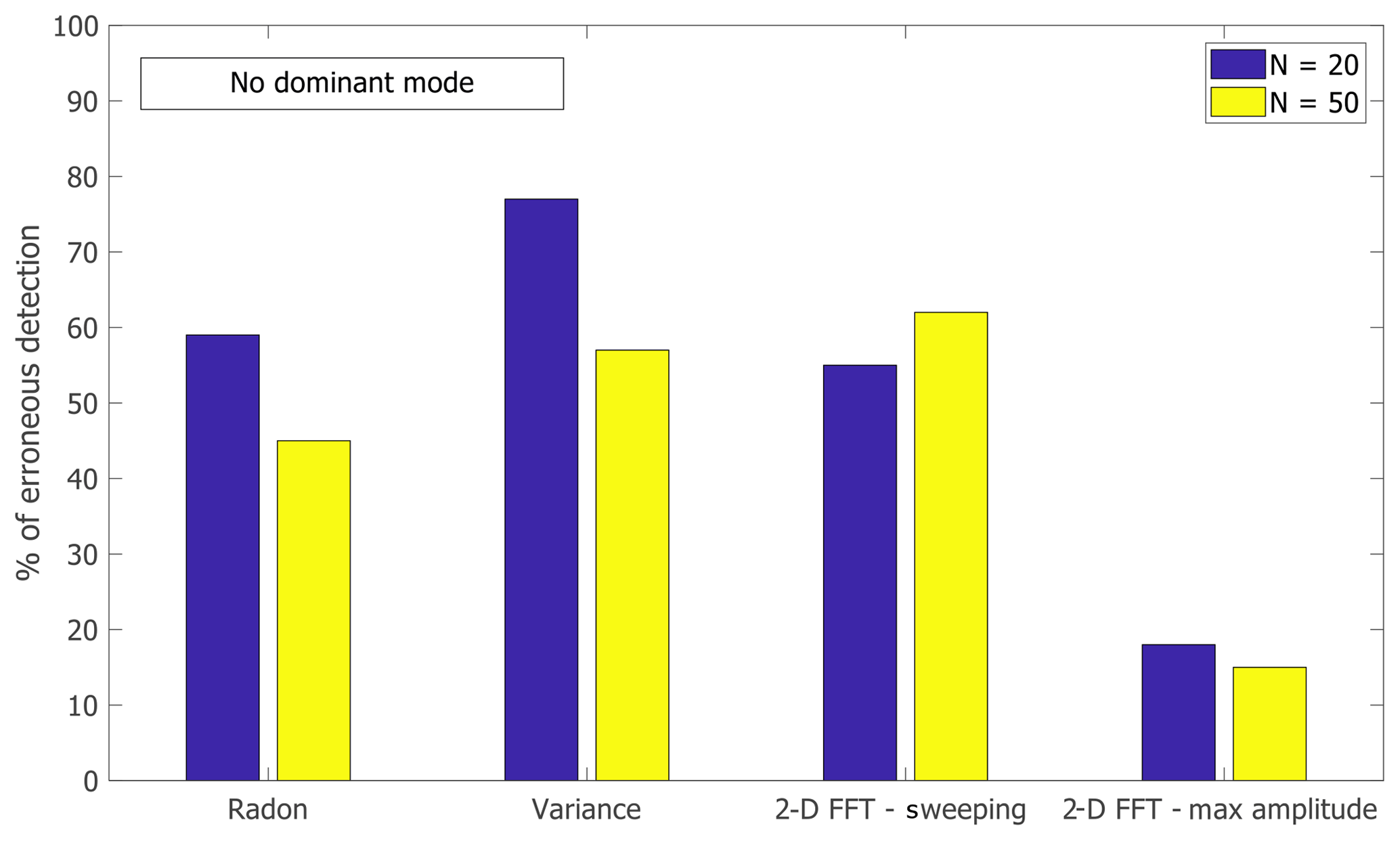
Figure 4 The percentage of erroneous detection of each variant of the methods when there is no dominant input amplitude.

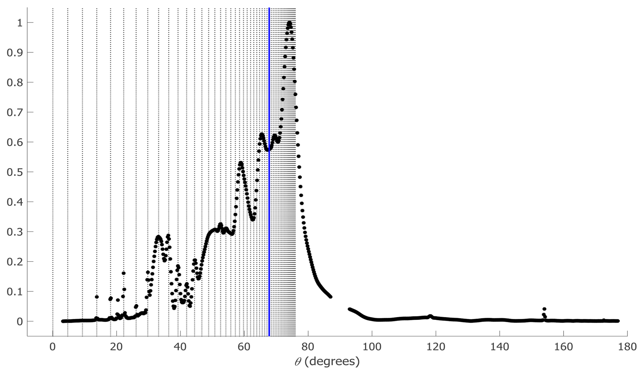
Figure 5 The distribution of the sum of squares of the Radon transform (black dots) versus the Radon angle θ. Clearly, the distribution of the corresponding input propagation speeds (vertical dashed black lines) as a function of θ is not uniform due to the nonlinear relation between C and θ.

The second test is a false-positive/true-negative test in which no dominant mode exists in the observed signal and a given method indicates that there exists a dominant mode (false-positive; FP) or not (true-negative; TN). In our case, this is done by generating a signal in which all modes have identical amplitudes (=1) and checking whether a method erroneously detects a certain propagation speed as dominant. If a dominant mode is detected, we assign it a score of 1 (“FP”), if a peak is detected but is too wide we assign it a score of 1∕2, and if there is no dominant mode (i.e., no distinct peak or more than one peak) we assign it a score of 0 (“TN”). We repeat this procedure 50 times for each of N=20 or N=50, sum up the scores and calculate the percentage of erroneous detection of a dominant mode in the signals by FP/(FP+TN)×100.

3 Results

An example of false determination of the dominant mode is shown in Fig. 2 for the signal shown in Fig. 1a. Figure 2a shows the distribution of the sum of squares of the Radon transform versus C (black markers), normalized such that the maximum value equals 1. Also plotted are the dashed black vertical lines located at the N values of the uniformly distributed propagation speeds, C, where the solid blue line is located at the C value of the dominant input mode's propagation speed. These dashed black and solid blue vertical lines are also shown Fig. 2b–d. Clearly, the dominant propagation speed calculated by the Radon transform (where the black curve attains its maximum) does not match the propagation speed of the dominant input mode. Figure 2b shows the (normalized) mean of variances as a function of C (black markers), and here, too, the calculated propagation speed (the curve's minimum point) does not agree with the dominant input mode's speed. Figure 2c shows the (normalized) distribution of the sum of squares of the spectral coefficients (2-D FFT-amplitudes) along different ω∕k lines (sweeping) as a function of C (black markers) where a distinct peak exists but it is located far from the dominant input mode's propagation speed. Figure 2d shows the 20 highest (normalized) 2-D FFT amplitudes of the (ω, k) diagram of Fig. 1b. There are many peaks with no clear single maximum, and the dominant input mode has one of the lowest amplitudes. For this signal, none of the methods correctly identified the dominant input mode.

The statistics of success of each method in detecting the dominant input mode for the TP/FN test is shown in Fig. 3 for dominant input mode's amplitude of 2.5, 5 and 10. The results for amplitudes of 1.5 and 2 are not shown as the success rate of all methods at these amplitudes is only between 10 % and 30 %. In each case we repeated the procedure 50 times (i.e., for 50 signals; note that there is no significant difference in the results if the number of repeats is changed to 25 or 100) for N=20 and then for N=50, summed the scores (1, 1∕2 or 0) and calculated the percentage of success by TP/(TP+FN)×100. The second scoring of 1, 2∕3, 1∕3, 0 yielded very similar numbers (up to 3 %) so they are not presented here. The conclusions from these results are as follows:

• in order to identify the dominant input mode with more than 70 % certainty, its amplitude should be larger than 5;

• no method has a clear advantage over the other methods;

• clearly, as N increases the dominant mode's amplitude has to increase, too, for a successful identification (so as to ensure that the ratio between the dominant mode's amplitude and the sum of all amplitudes is similar for different values of N since, e.g., 2.5/20 > 2.5/50); and

• the minimal amplitude at which successful detection occurs, decreases with the decrease in the ranges of propagation speeds and periods. Thus, for propagation speeds in the range of −10 to −2 cm s⁻¹ and periods between 15 and 100 weeks, an amplitude of 5 is successfully detected in over 90 % of the cases, while an amplitude of 2 yields poor results (results not shown).

The statistics of erroneous detection of a dominant mode (the FP/TN test where the amplitudes of all input modes equal 1 i.e., there is no dominant input mode) is shown in Fig. 4 for each of the methods (here, again, we have generated 50 signals for N=20 and for N=50 and calculated the percentage of erroneous detection by FP/(FP+TN)×100). The 2-D FFT maxima method is the only method for which the percentage of error is smaller than 20 % while the other three methods err in at least 50 % of the cases (i.e., they identify a single clear peak in one of the propagation speeds). As N increases this erroneous detection percentage decreases slightly in the two Radon variants but increases slightly in the 2-D FFT sweeping method.

4 Discussion

None of the methods can identify a dominant input mode unless its amplitude is significantly larger than the others (by a factor larger than five in the present study's ranges of propagation speeds and periods) and most of them (except the 2-D FFT maxima) erroneously detect a dominant mode when there is no such input mode. Though the 2-D FFT maxima method does not falsely detect dominant mode when it does not exist, its performance in detecting a dominant input mode when it exists is not satisfactory. For realistic signals in the ocean we do not know that there is a dominant mode with sufficiently large amplitude so none of the methods is reliable for estimating the propagation speed of e.g., Rossby waves.

When the values of ω and k are chosen in a range corresponding to the resolution limit and the Nyquist frequency, the success of 2-D FFT in identifying the dominant input mode's propagation speed increases significantly, compared to the case where the values of C are determined in advance, ω is chosen randomly in a particular range and k is set to ω∕C so aliasing can occur. For that reason, even if the signal includes only one mode (i.e., one C), and both ω and k are chosen in the latter manner, there can be a wrong identification by the 2-D FFT (but the Radon transform identifies it correctly). In the ocean we do not know ab initio which wavenumbers and frequencies exist so we cannot filter them out of the signal; hence aliasing can occur, and the percentage of success in detecting the real dominant mode is expected to decrease further.

The erroneous identification of the Radon and variance methods can be partially attributed to the non-linear relation between the angle θ and the propagation speed, C, which is proportional to tan(θ), so the equidistant values of C are converted to θ values that are very close to one another. Figure 5 shows the distribution of the sum of squares of the Radon transform versus θ for the signal shown in Fig. 1a (while the distribution of the sum of squares of the Radon transform versus C for that signal is shown in Fig. 2a). It is clear from this figure that the peak is located in the vicinity of θ values corresponding to many C values. However, the performance of the Radon variants improves with the increase of the dominant input mode's amplitude, so the non-linear relation between the angle and propagation speed is not the only reason for the mismatch.

As N (the number of modes) increases, the dominant input mode's amplitude should be larger in order to be separately identified from modes with similar characteristics. Of course, in the real ocean it is impossible to establish a priori a bound on the number of modes, on the width of the bins (which becomes narrower as N increases), and on the expected maximal amplitude, so fewer results can be evaluated as success. Also, in narrower ranges of propagation speeds and periods and for the same number of bins, all methods correctly detect the dominant input mode at lower-threshold amplitudes (results not shown). An implication of this finding for the detection of the dominant mode in the ocean is that a reliable estimate of the phase speed cannot be based on a single method (see also De-Leon and Paldor, 2017a).

In addition to the amplitude of the dominant input mode and its width, a parameter that might affect the success of detection of the dominant mode is the existence of a cluster of dominant input modes with similar phase speeds. This was ignored in the results presented above where in all repeats there was a single dominant input mode. To examine this aspect, we generated a signal made of 20 modes, out of which a triplet of adjacent, randomly selected, modes had amplitudes of (2, 4, 2) instead of a single mode with an amplitude of 5. The statistics of repeats showed that all methods have detected the dominant mode with slightly elevated confidence (less than 10 % higher) in the former cluster of modes, compared to the latter single mode (results not shown). Though the sum of the squares of the amplitudes of the cluster is smaller than the squared amplitude of the single mode (i.e., ${\mathrm{2}}^{\mathrm{2}}+{\mathrm{4}}^{\mathrm{2}}+{\mathrm{2}}^{\mathrm{2}}=\mathrm{24}<\mathrm{25}={\mathrm{5}}^{\mathrm{2}}$), the linear sum of the amplitudes of the cluster is larger than that of the single mode (i.e., $\mathrm{2}+\mathrm{4}+\mathrm{2}=\mathrm{8}>\mathrm{5}$), so the elevated amplitude rather than the square of the amplitude might explain the improved detection of the cluster. An examination of this “clustering” effect in a signal made up of a continuous unbounded spectrum of phase speeds (i.e., N→∞), which better models the real ocean, is left for future work.

The weakness of the methods in identifying the dominant mode points to the difficulty in comparison between theories and observations of baroclinic Rossby waves in the ocean, and this difficulty might explain the lack of continuity of propagation speed estimates between adjacent latitudes in one or more methods. It can also explain why a validation of the higher-order trapped wave theory (where the β term is treated consistently) has been confirmed by observations only in the Indian Ocean south of Australia (De-Leon and Paldor, 2017b) and not in other parts of the world ocean. In contrast to the harmonic theory whose propagation speed estimates are always slower than the observed speeds, the trapped wave theory differs from observations sporadically (see Fig. 5 of De-Leon and Paldor, 2017b).