Internal tide energy flux over a ridge measured by a co-located ocean glider and moored acoustic Doppler current profiler

Internal tide energy flux is an important diagnostic for the study of energy pathways in the ocean, from large-scale input by the surface tide to small-scale dissipation by turbulent mixing. Accurate calculation of energy flux requires repeated full-depth measurements of both potential density (ρ) and horizontal current velocity (u) over at least a tidal cycle and over several weeks to resolve the internal spring–neap cycle. Typically, these observations are made using full-depth oceanographic moorings that are vulnerable to being “fished out” by commercial trawlers when deployed on continental shelves and slopes. Here we test an alternative approach to minimize these risks, with u measured by a low-frequency acoustic Doppler current profiler (ADCP) moored near the seabed and ρ measured by an autonomous ocean glider holding station by the ADCP. The method is used to measure the semidiurnal internal tide radiating from the Wyville Thomson Ridge in the North Atlantic. The observed energy flux (4.2±0.2 kW m⁻¹) compares favourably with historic observations and a previous numerical model study.

Error in the energy flux calculation due to imperfect co-location of the glider and ADCP is estimated by subsampling potential density in an idealized internal tide field along pseudorandomly distributed glider paths. The error is considered acceptable (<10 %) if all the glider data are contained within a “watch circle” with a diameter smaller than 1∕8 the mode-1 horizontal wavelength of the internal tide. Energy flux is biased low because the glider samples density with a broad range of phase shifts, resulting in underestimation of vertical isopycnal displacement and available potential energy. The negative bias increases with increasing watch circle diameter. If watch circle diameter is larger than 1∕8 the mode-1 horizontal wavelength, the negative bias is more than 3 % and all realizations within the 95 % confidence interval are underestimates. Over the Wyville Thomson Ridge, where the semidiurnal mode-1 horizontal wavelength is ≈100 km and all the glider dives are within a 5 km diameter watch circle, the observed energy flux is estimated to have a negative bias of only 0.4 % and an error of less than 3 % at the 95 % confidence limit. With typical glider performance, we expect energy flux error due to imperfect co-location to be <10 % in most mid-latitude shelf slope regions.

1 Introduction

Internal tides are a ubiquitous hydrodynamic feature over continental shelves and slopes as they are commonly generated at the shelf break by across-slope tidal flows (Baines, 1982; Pingree et al., 1986; Sharples et al., 2007). However, direct measurement of internal tides can be a challenge in these regions due to intense commercial fishing activity leading to an increased risk of oceanographic mooring loss (Sharples et al., 2013). Calculation of internal tide energy flux, a key diagnostic for the understanding of baroclinic energy pathways, requires repeated full-depth measurements of both potential density (ρ) and horizontal current velocity (u) over at least a tidal cycle (Nash et al., 2005). If an objective is to resolve the internal spring–neap cycle or observe the effect of seasonal changes in stratification on the internal tide field, repeated full-depth measurements over several weeks or months are required. Typically, these measurements are made using a full-depth oceanographic mooring incorporating an acoustic Doppler current profiler (ADCP) and a string of conductivity–temperature loggers (e.g. Hopkins et al., 2014), or a profiling mooring with a CTD (conductivity, temperature, and depth) and acoustic current meter (e.g. Zhao et al., 2012). On continental shelves and slopes, these full-depth moorings are vulnerable to being “fished out” by demersal and pelagic trawling activity.

Hall et al. (2017b) describe a novel alternative approach to minimize these risks, with u measured by a low-frequency ADCP moored near the seabed and ρ measured by an autonomous ocean glider holding station by the ADCP as a “virtual mooring”. Commercial fishing activity on continental shelves and their adjacent slopes is often intense because these regions are highly biologically productive. However, steps can be taken to reduce the risk of ADCP loss, including deploying deeper than 600 m, keeping mooring lines short, or using trawl-resistant frames. Being relatively small, gliders are unlikely to be fished out, and the risk can be further reduced by real-time evasive action in response to vessel proximity guided by the maritime automatic identification system (AIS). However, this alternate approach was not comprehensively tested by Hall et al. (2017b) because of glider navigation and telemetry problems. In this study we test the method using a co-located glider and ADCP dataset from the Wyville Thomson Ridge in the North Atlantic, a topographic feature that previous observations and numerical model studies suggest is an energetic internal tide generator (Sherwin, 1991; Hall et al., 2011). We also estimate the error in the energy flux calculation due to imperfect co-location of the glider and ADCP and find that, with typical glider performance, it is acceptable in most mid-latitude shelf slope regions.

Ocean gliders have previously been used to observe internal waves and internal tides (Rudnick et al., 2013; Rainville et al., 2013; Johnston and Rudnick, 2015; Boettger et al., 2015; Hall et al., 2017a), including the calculation of energy fluxes using current velocity measurements from gliders equipped with ADCPs (Johnston et al., 2013, 2015). However, ADCPs are not routinely integrated with commercially available glider platforms (Seaglider, Slocum, and SeaExplorer), in part due to their higher power requirement. Synergy with moored ADCP data allows accurate calculation of internal tide energetics without the endurance limitations and data analysis complexities of an ADCP-equipped glider (e.g. Todd et al., 2017).

In Sect. 2 the temporal resolution constraints of glider measurements are explained and the observations used in this study described. The calculation of internal tide energy flux from co-located glider and moored ADCP data is fully described in Sect. 3. Observations of the internal tide radiating from the Wyville Thomson Ridge are presented in Sect. 4 and compared with historic observations and a previous numerical model study. In Sect. 5 the error in the energy flux calculation due to imperfect co-location is estimated. Key results are summarized and discussed in Sect. 6.

2 Observations

Figure 1 (a) Location of the experiment site (white square) and regional bathymetry, including the Faroe Bank Channel (FBC), Faroe–Shetland Channel (FSC), and Wyville Thomson Ridge (WTR). (b) Path of the glider over the WTR with local bathymetry (Δ50 m isobaths in grey). Dives are separated into deployment (red), on-station (magenta), and recovery (blue) sections with a black cross every 12 h (00:00 and 12:00 UTC). The dotted black lines are surface drift. The white triangle is the location of the ADCP mooring and the dashed white line delineates a 5 km diameter “watch circle” around it. The white circle is the location of the CTD repeat station where Sherwin (1991) observed a semidiurnal internal tide. The bathymetric dataset is the GEBCO 2014 30 arcsec grid (http://www.gebco.net, last access: 25 March 2015).

High temporal resolution is crucial for internal tide observations; Nash et al. (2005) suggest that a minimum of four evenly distributed independent profiles of u and ρ are required per tidal cycle for an unbiased calculation of energy flux. Over continental shelves and upper shelf slopes, this temporal resolution is achievable using gliders. Typical glider vertical velocities are 15–20 cm s⁻¹, so a complete dive cycle to 1000 m can take as little as 3 h. This yields eight profiles (four dives) per semidiurnal (≈12 h) tidal cycle, but near the surface and seabed the descending and ascending profiles converge in time so the number of independent samples is halved to four. For diurnal (≈24 h) internal tides, 16 profiles per cycle are possible. In shallower water the temporal resolution of glider measurements increases further; 40 min full-depth dives are achievable over a 200 m deep shelf break, yielding 36 profiles per semidiurnal tidal cycle. The depth-limiting factor of the methodology is the range of the ADCP. In narrowband mode, 75 kHz ADCPs have a maximum range of around 600 m (dependent on environmental conditions) so multiple ADCPs or additional current meters on the mooring line are required for sites between 600 and 1000 m deep.

The observations used to test the method were collected from the northern flank of the Wyville Thomson Ridge (WTR) in the North Atlantic (Fig. 1a). A Kongsberg Seaglider (SG613; Eriksen et al., 2001) was deployed from NRV Alliance between 2 and 5 June 2017 during the fourth Marine Autonomous Systems in Support of Marine Observations mission (MASSMO4). The glider was navigated from the deeper waters of the Faroe–Shetland Channel (FSC) to the WTR and held station for 40 h by a short oceanographic mooring, deployed 5 days previously from MRV Scotia (Fig. 1b). The mooring was sited close to the 800 m isobath and instrumented with an upwards-looking 75 kHz RDI Long Ranger ADCP at approximately 722 m and an Aanderaa Seaguard acoustic current meter at 784 m, yielding observations of horizontal current velocity over 78 % of the water column. When on-station by the ADCP mooring, the glider made repeated 2 h dives to 700 m or the seabed, whichever was shallower. This yielded approximately 12 profiles (six independent samples near the surface and seabed; 12 independent samples at mid-depth) per semidiurnal tidal cycle.

Glider location at the surface, before and after each dive, was given by GPS position. Subsurface sample locations were approximated by linearly interpolating surface latitude and longitude onto sample time. When on-station, the glider stayed within 2.5 km of the mooring and the mean horizontal distance between temporally coincident glider and ADCP measurements was 1.3 km. This spatial scattering of the glider data is small compared to the semidiurnal mode-1 horizontal wavelength over the WTR (≈100 km, calculated from the observed buoyancy frequency profile) and so the glider data are initially considered a fixed-point time series with no spatial–temporal aliasing.

As the glider was on-station for only 40 h, the co-located time series is not long enough to resolve the internal spring–neap cycle. As a result, M₂ harmonic fits to the glider and mooring data (Sect. 3) are contaminated with S₂ variability. To acknowledge this, we refer to the estimated M₂ component of the co-located time series as D₂ following Alford et al. (2011). The comparative numerical model (Sect. 4.1) only includes the M₂ tidal constituent so we refer to model diagnostics as M₂.

2.1 Data processing

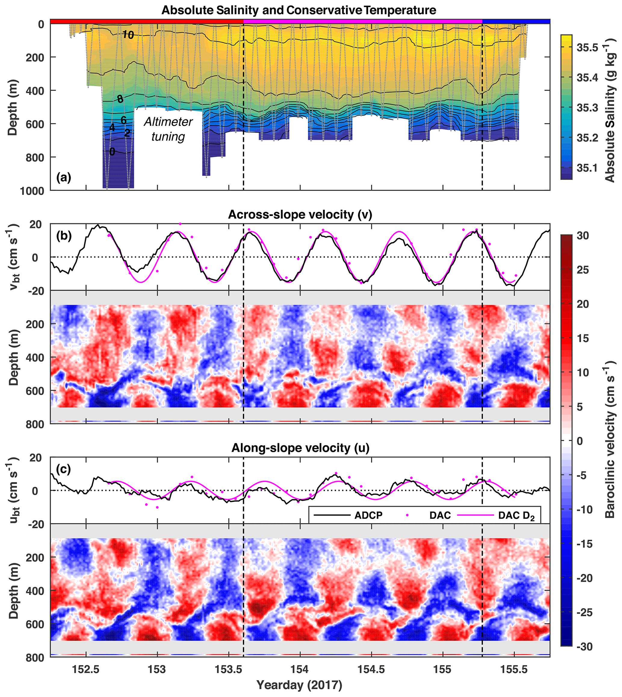
Figure 2 (a) Absolute Salinity (colour) and Conservative Temperature (black contours, interval: 1 ^∘C) measured by the glider. The dotted grey line is the glider's path and shows the temporal sampling resolution. The magenta section is when the glider was on-station by the ADCP mooring. (b) Across-slope barotropic (black line) and baroclinic (colour) velocities measured by the ADCP and current meter and dive-average current (DAC) velocity inferred from the glider (magenta dots). The magenta line is a D₂ harmonic fit to DAC velocity. Positive velocities are northeast (down-slope). Panel (c) is the same as (b) but for along-slope velocities. Positive velocities are southeast.

The glider was equipped with a standard Sea-Bird Electronics conductivity–temperature (CT) sail sampling at 0.2 Hz and the data processed using the UEA Seaglider Toolbox (https://bitbucket.org/bastienqueste/uea-seaglider-toolbox, last access: 9 February 2017) following Queste (2014). Conductivity data were corrected for thermal hysteresis following Garau et al. (2011) and the Seaglider flight model regressed using a method adapted from Frajka-Williams et al. (2011). As the CT sail was unpumped, salinity samples were flagged when the glider's speed was less than 10 cm s⁻¹ or it was within 8 m of apogee¹. Temperature–salinity profiles from descents and ascents were independently averaged (median value) in 5 m depth bins, typically with 4–5 samples per bin. Sample time was averaged into the same bins to allow accurate temporal analysis at all depths. Absolute Salinity (S_A), Conservative Temperature (Θ), and potential density (ρ) in each bin were calculated using the TEOS-10 equation of state (IOC et al., 2010).

The 75 kHz ADCP was configured in narrowband mode with 10 m bins and 24 pings per 20 min ensemble. The ADCP data were processed using Marine Scotland Science's standard protocols, including correction for magnetic declination and quality assurance based on error velocity, vertical velocity, and percentage good ping thresholds. The ADCP data were then linearly upsampled onto the same Δ5 m depth levels as the glider data. The acoustic current meter was configured with a 10 min sampling interval and linearly downsampled onto the same 20 min sampling interval as the ADCP. Good velocity data were recovered for all depth levels between 85 and 705 m, as well as 780–785 m. In addition to the ADCP and current meter measurements, horizontal velocity was inferred from GPS position and the Seaglider flight model using a dive-average current method (DAC; Eriksen et al., 2001; Frajka-Williams et al., 2011). DAC was only calculated for dives deeper than 500 m so that values were representative of the majority of the water column. All velocities were transformed into along-slope and across-slope components. We take the northern flank of the WTR to be orientated exactly northwest–southeast so along-slope (u) is positive southeast and across-slope (v) is positive northeast (down-slope).

The full 3-day glider time series of Conservative Temperature and Absolute Salinity is shown in Fig. 2a. A semidiurnal internal tide is evident as a vertical oscillation of the main pycnocline (centred around 550 m) with an amplitude up to 50 m and a period of ≈12 h. Temporally coincident ADCP and current meter measurements (Fig. 2b, c) show dominant semidiurnal periodicity and a reversal of baroclinic current velocity across the main pycnocline, characteristic of a low-mode internal tide. Mode-1 horizontal velocity, calculated from the observed buoyancy frequency profile, reverses at approximately 505 m, slightly above the pycnocline.

3 Internal tide energy flux

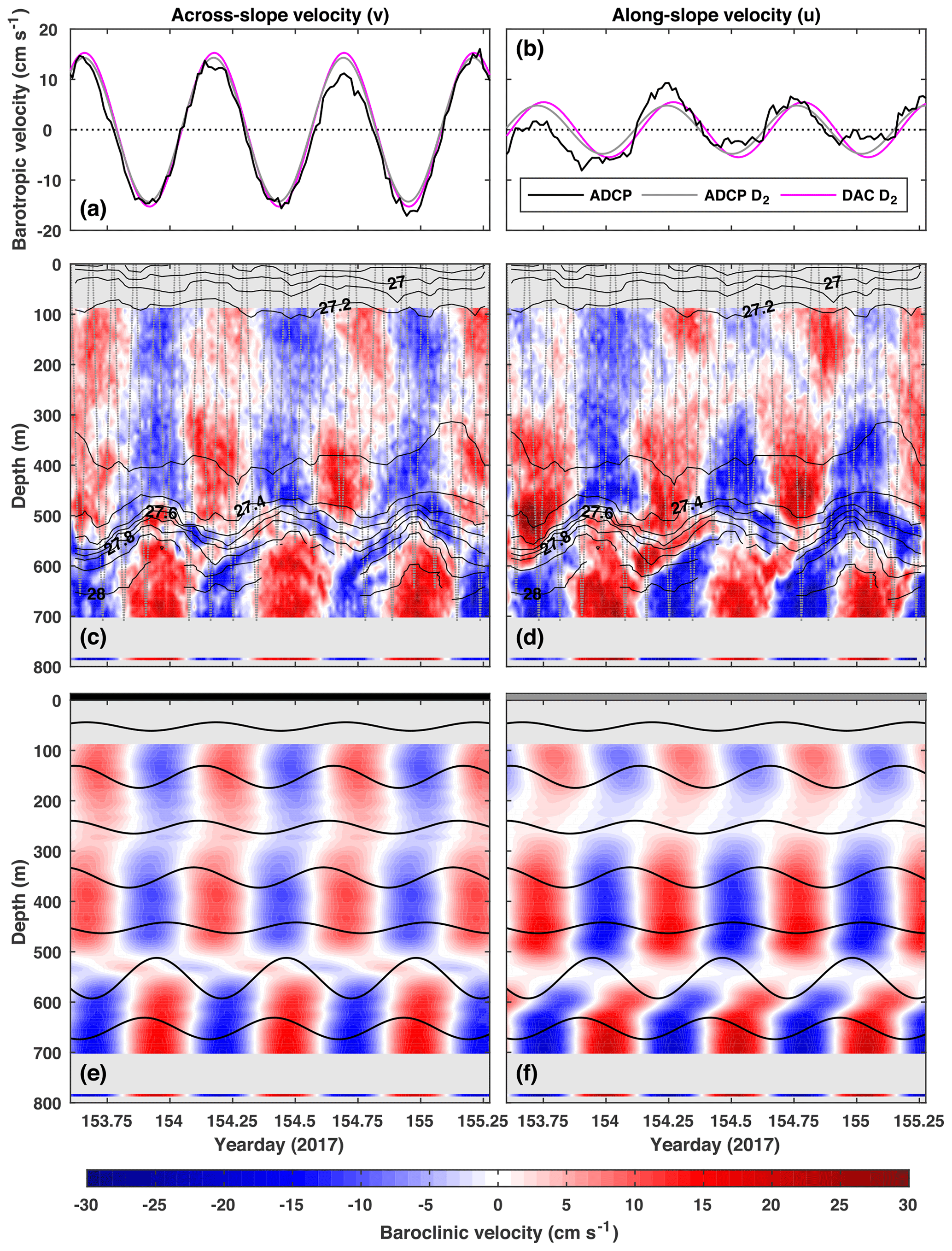
Figure 3 (a) Across-slope barotropic velocity (black), the D₂ component (grey), and a D₂ harmonic fit to DAC velocity (magenta). (c) Across-slope baroclinic velocity (colour) overlaid with potential density (black contours, interval: 0.1 kg m⁻³). (e) The D₂ component of across-slope baroclinic velocity (colour) overlaid with the D₂ component of vertical isopycnal displacement every 100 m (black lines). Panels (b), (d), and (f) are the same as (a), (c), and (e) but for along-slope velocities.

Figure 4 (a) Amplitude and (b) phase of the D₂ components of across-slope baroclinic velocity (black), along-slope baroclinic velocity (grey), and vertical isopycnal displacement (magenta). (c) Horizontal kinetic energy (black), available potential energy (magenta), and buoyancy frequency squared (green). (d) Across-slope (black) and along-slope (grey) D₂ internal tide energy flux. Solid lines indicate both glider and ADCP data coverage; dashed lines indicate that one or both of the datasets required extrapolation. Positive fluxes are down-slope and along-slope to the southeast.

Following Kunze et al. (2002) and Nash et al. (2005), internal tide energy flux is calculated as $\mathit{F}=〈{\mathit{u}}_{\mathrm{bc}}^{\prime }{p}^{\prime }〉$. The method requires repeated full-depth measurements of ρ and u over at least a tidal cycle in order to determine pressure perturbation (p^′) and baroclinic velocity (${\mathit{u}}_{\mathrm{bc}}^{\prime }$), respectively.

3.1 Pressure perturbation

For the 40 h window when the glider was on-station by the ADCP mooring, potential density anomaly is calculated by subtracting the window-mean density profile from measured potential density,

$$\begin{array}{}\text{(1)}& {\mathit{\rho }}^{\prime }(z,t)=\mathit{\rho }(z,t)-\stackrel{\mathrm{‾}}{\mathit{\rho }}\left(z\right).\end{array}$$

Before subtraction, $\stackrel{\mathrm{‾}}{\mathit{\rho }}\left(z\right)$ is smoothed with a 50 m gaussian tapered running mean (σ=10 m) to yield a suitable background density profile. Vertical isopycnal displacement is then calculated as

$$\begin{array}{}\text{(2)}& \mathit{\xi }(z,t)=-{\mathit{\rho }}^{\prime }(z,t){\left({\displaystyle \frac{\partial \stackrel{\mathrm{‾}}{\mathit{\rho }}}{\partial z}}\right)}^{-\mathrm{1}}.\end{array}$$

To separate D₂ internal tide variability from other physical processes, M₂ tidal period (T=12.42 h) harmonics are fit to ξ on each Δ5 m depth level following Emery and Thomson (2001). This analysis is only applied to depth levels between 10 and 675 m; near-surface and near-bottom bins are excluded because of high numbers of flagged samples and reduced temporal resolution due to the glider going into apogee above 700 m. To obtain a full-depth time series, the D₂ component of ξ is linearly extrapolated assuming ξ=0 at the surface (z=0) and bottom ($z=-H$, where H is water depth). Buoyancy frequency squared, $N^{\mathrm{2}}=-g/{\mathit{\rho }}_{\mathrm{0}}(\partial \stackrel{\mathrm{‾}}{\mathit{\rho }}/\partial z)$, is also linearly extrapolated, assuming $N^{\mathrm{2}}={\mathrm{10}}^{-\mathrm{6}}$ s⁻² at the surface and bottom. Pressure perturbation is then calculated by integrating the hydrostatic equation from the surface,

$$\begin{array}{}\text{(3)}& p^{\prime }(z,t)=p_{\mathrm{surf}}^{\prime }\left(t\right)+{\mathit{\rho }}_{\mathrm{0}}\underset{z}{\overset{\mathrm{0}}{\int }}{N}^{\mathrm{2}}\left(z\right)\mathit{\xi }(z,t)\mathrm{d}z,\end{array}$$

where $p_{\mathrm{surf}}^{\prime }$ is pressure perturbation at the surface due to the internal tide, determined by applying the baroclinicity condition for pressure,

$$\begin{array}{}\text{(4)}& p_{\mathrm{surf}}^{\prime }\left(t\right)=-{\displaystyle \frac{\mathrm{1}}{H}}\underset{-H}{\overset{\mathrm{0}}{\int }}{p}^{\prime }(z,t)\mathrm{d}z.\end{array}$$

Figure 3 shows potential density (Fig. 3c and d) and the D₂ component of vertical isopycnal displacement (Fig. 3e and f) for the 40 h analysis window. The amplitudes and phases of the D₂ component of ξ are shown in Fig. 4a and b.

3.2 Baroclinic velocity

For the same 40 h window, horizontal velocity perturbation is calculated,

$$\begin{array}{}\text{(5)}& {\mathit{u}}^{\prime }(z,t)=\mathit{u}(z,t)-\stackrel{\mathrm{‾}}{\mathit{u}}\left(z\right),\end{array}$$

where $\stackrel{\mathrm{‾}}{\mathit{u}}\left(z\right)$ is the window-mean horizontal velocity profile. There are three spatial gaps in the time series: above 85 m, between the ADCP and current meter (705–780 m including blanking distance), and from the current meter to the seabed (785–800 m). To obtain a full-depth time series, u^′ is linearly interpolated between the ADCP and current meter, and extrapolated to the surface and the bottom using a nearest neighbour method. Baroclinic velocity is then calculated,

$$\begin{array}{}\text{(6)}& {\mathit{u}}_{\mathrm{bc}}^{\prime }(z,t)={\mathit{u}}^{\prime }(z,t)-{\mathit{u}}_{\mathrm{bt}}^{\prime }\left(t\right),\end{array}$$

where ${\mathit{u}}_{\mathrm{bt}}^{\prime }$ is barotropic velocity, assumed here to equal the depth-mean velocity, calculated as

$$\begin{array}{}\text{(7)}& {\mathit{u}}_{\mathrm{bt}}^{\prime }\left(t\right)={\displaystyle \frac{\mathrm{1}}{H}}\underset{-H}{\overset{\mathrm{0}}{\int }}{\mathit{u}}^{\prime }(z,t)\mathrm{d}z.\end{array}$$

The D₂ components of ${\mathit{u}}_{\mathrm{bc}}^{\prime }$ and ${\mathit{u}}_{\mathrm{bt}}^{\prime }$ are extracted using the same harmonic analysis method applied to ξ. Figure 3 shows barotropic (Fig. 3a and b) and baroclinic (Fig. 3c and d) velocities and the D₂ components of barotropic (Fig. 3a and b) and baroclinic (Fig. 3e and f) velocities for the 40 h analysis window. The amplitudes and phases of the D₂ component of ${\mathit{u}}_{\mathrm{bc}}^{\prime }$ are shown in Fig. 4a and b.

3.3 Internal tide energetics

Profiles of internal tide energy flux, available potential energy (APE), and horizontal kinetic energy (HKE) are calculated as

$$\begin{array}{}\text{(8)}& {\displaystyle }& {\displaystyle }\mathit{F}\left(z\right)=〈{\mathit{u}}_{\mathrm{bc}}^{\prime }(z,t)p^{\prime }(z,t)〉,\text{(9)}& {\displaystyle }& {\displaystyle }\mathrm{APE}\left(z\right)={\displaystyle \frac{\mathrm{1}}{\mathrm{2}}}{\mathit{\rho }}_{\mathrm{0}}{N}^{\mathrm{2}}\left(z\right)〈{\mathit{\xi }}^{\mathrm{2}}(z,t)〉,\end{array}$$

and

$$\begin{array}{}\text{(10)}& \mathrm{HKE}\left(z\right)={\displaystyle \frac{\mathrm{1}}{\mathrm{2}}}{\mathit{\rho }}_{\mathrm{0}}〈{\mathit{u}}_{\mathrm{bc}}^{\prime \mathrm{2}}(z,t)〉,\end{array}$$

where 〈⋅〉 denotes an average (mean) over an integer number of M₂ cycles and ρ₀=1028 kg m⁻³ is a reference density.

4 Results

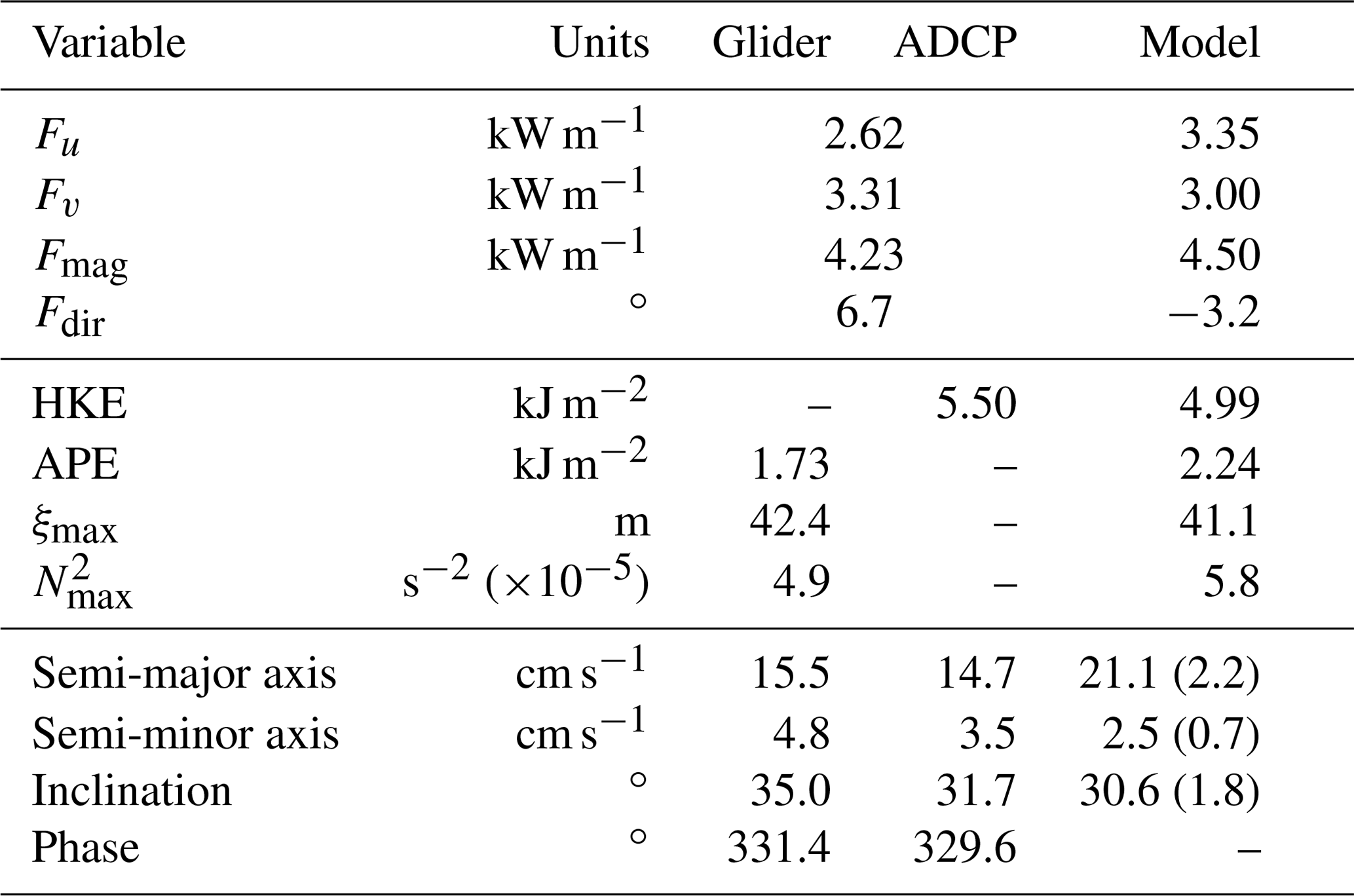
Maximum D₂ vertical isopycnal displacement is 42 m and occurs at 565 m (Fig. 4a), within the main pycnocline. This is comparable with historic observations of a semidiurnal internal tide over the northern flank of the WTR. Sherwin (1991) analysed CTD data from a 17 h repeat station (30 min between casts) that was 6.7 km east of the mooring (Fig. 1b) and determined maximum D₂ vertical isopycnal displacement to be 37 at 580 m, again within the pycnocline. Here, almost all of the APE is contained within the pycnocline (Fig. 4c) because maximum ξ occurs at a similar depth to maximum N² ($\mathrm{4.9}\times {\mathrm{10}}^{-\mathrm{5}}$ s⁻² at 525 m). D₂ baroclinic velocity is maximum (≈20 cm s⁻¹) near-bottom (Fig. 4a), as is HKE (Fig. 4c). Depth-integrated HKE and APE are 5.5 and 1.7 kJ m⁻², respectively.

Both the across- and along-slope components of D₂ internal tide energy flux are maximum (≈12.7 kW m⁻²) near-bottom and go to zero at the depth of maximum N² (Fig. 4d), characteristic of a low-mode internal tide with a pycnocline in the lower half of the water column. Depth-integrated energy flux magnitude is 4.2 kW m⁻¹, directed almost due east (7^∘ anticlockwise from east). In comparison, Sherwin (1991) estimated the D₂ mode-1 internal tide energy flux at the nearby CTD repeat station to be 4.7 kW m⁻¹, but was unable to diagnose the direction.

4.1 Model comparison

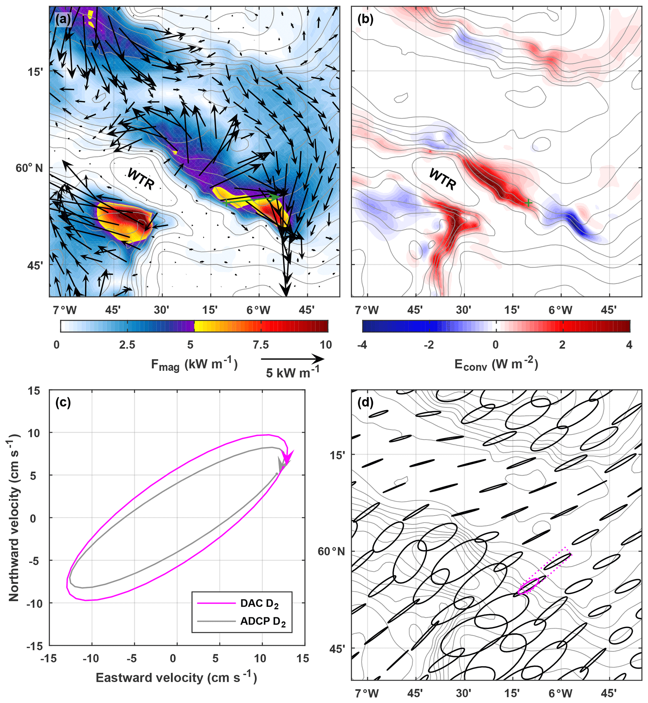
Figure 5 (a) Depth-integrated M₂ internal tide energy flux from the regional tide model described by Hall et al. (2011). Vectors are plotted every five grid points (5 km) in each direction. The underlying colour is the energy flux magnitude. The green vector is the depth-integrated D₂ internal tide energy flux observed at the green cross. (b) Barotropic-to-baroclinic M₂ energy conversion from the model. (c) D₂ surface ellipses calculated from glider-inferred DAC velocity (magenta) and ADCP-measured barotropic velocity (grey). (d) M₂ surface ellipses, every 10 grid points (10 km) in each direction, from the model. The magenta ellipse is calculated from DAC velocity and is representative of the area that contains all the dives deeper than 500 m (delineated by the dotted magenta line). The bathymetry contour interval is 100 m.

Table 1 Comparison between observed (glider and ADCP) D₂ and modelled M₂ internal tide and surface tidal ellipse diagnostics. Modelled ellipse values are averaged (mean) over the 48 grid points in the area that contains all the glider dives deeper than 500 m (see Fig. 5d). The values in brackets are standard deviations. All bearings are anticlockwise from east.

In Fig. 5 the observations are compared with the regional tide model described by Hall et al. (2011). The model is a configuration of the Princeton Ocean Model (POM; Blumberg and Mellor, 1987) for the FSC and WTR region, initiated with typical late-summer stratification and forced at the boundaries with M₂ barotropic velocities (see Hall et al., 2011, for full details). Maximum N² in the model is slightly higher than observed (Table 1) but the vertical distribution of stratification is similar; the main pycnocline is between 500 and 600 m. M₂ internal tide generation occurs within the model domain, driven by barotropic tidal currents across isobaths, and is diagnosed as positive barotropic-to-baroclinic energy conversion (Fig. 5b). The northern flank of the WTR is an area of energetic internal tide generation, up to 4 W m⁻², and radiates an internal tide into the southern FSC. Modelled internal tide energy fluxes are spatially variable, but >5 kW m⁻¹ at some locations (Fig. 5a). The mooring was located east of the most energetic generation and up-slope of the largest energy fluxes.

For direct comparison, the model output is interpolated onto the exact location of the mooring (Table 1). The modelled M₂ internal tide energy flux is 6 %–7 % larger than the observed D₂ energy flux, but within 10^∘ of its direction. Maximum modelled vertical isopycnal displacement is 41 m (slightly smaller than observed) but is compensated by the higher maximum N² and results in modelled APE being 30 % larger than observed; modelled HKE is 10 % smaller than observed.

4.2 Surface tidal ellipses

As well as measuring potential density by the ADCP mooring, the glider is used to infer a second estimate of barotropic velocity. Harmonic analysis is used to extract the D₂ component of DAC velocity (all dives deeper than 500 m) and compared to the D₂ component of ${\mathit{u}}_{\mathrm{bt}}^{\prime }$ from the ADCP and current meter. Barotropic velocity is highest in the across-slope direction (maximum 15 cm s⁻¹; Fig. 3a) and there is a very close match between the DAC and ADCP estimates (rms difference is 0.8 cm s⁻¹). In the along-slope direction, where barotropic velocity is lower (maximum 0.5 cm s⁻¹; Fig. 3b), the DAC estimate lags the ADCP estimate by 35 min but their amplitudes closely match (rms difference is 1.2 cm s⁻¹). The resulting surface tidal ellipses have similar semi-major axis lengths and phases (Table 1) but the DAC estimate is less eccentric (more circular) and rotated 3^∘ anticlockwise (Fig. 5c). Compared with M₂ surface ellipses from the regional tide model described by Hall et al. (2011), both observational estimates are less eccentric and have shorter semi-major axes (Table 1; Fig. 5c). However, the inclination of observed and modelled ellipses are comparable, with their semi-major axes orientated across-slope. This is the orientation required to generate an energetic internal tide at the WTR.

5 Glider sampling error

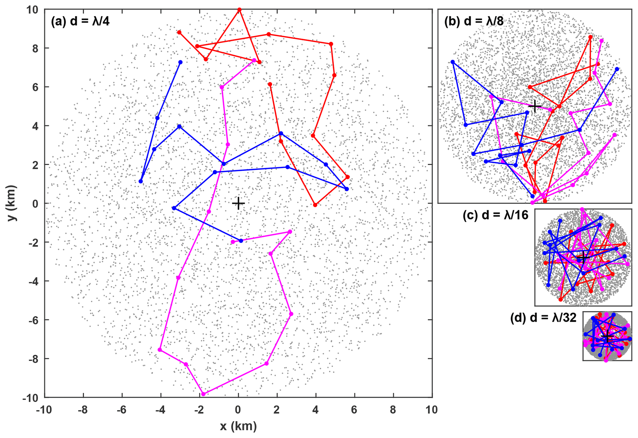
Figure 6 Pseudorandomly distributed glider paths within watch circles of diameters (a) 1∕4λ, (b) 1∕8λ, (c) 1∕16λ, and (d) 1∕32λ. The first 5000 surface locations are shown with a grey dot and the first three twelve-dive scenarios are shown in colour. The black cross is the location of the ADCP at the centre of the watch circle. All four panels are the same scale.

The separation of spatial and temporal variability is a common problem when interpreting glider data due to their slow speed (Rudnick and Cole, 2011) and imperfect positioning. In this context, the inability of the glider to perfectly hold station by the ADCP mooring leads to error in the calculation of internal tide energy flux (Sect. 3) due to mis-sampling of the spatially and temporally varying density field. An understanding of this error is important for both mission planning and interpretation of results. Other missions along the European continental slope (e.g. Hall et al., 2017a) have shown that a glider operating as a virtual mooring by repeatedly diving to 1000 m around a fixed station can maintain a “watch circle” with a diameter of approximately 5 km, i.e. all dives start and end within 2.5 km of the target location. The ability to do this is dependent on environmental conditions, particularly tidal and slope currents, but the lower limit is effectively set by the glide angle; a steep 45^∘ glide angle will result in around 2 km horizontal travel over a complete dive cycle to 1000 m.

The size of the energy flux error is related to the length scale of the sampling cloud (d, the diameter of the watch circle) and the horizontal wavelength of internal tide being measured (λ). If d≪λ we can consider the glider data a fixed-point time series with no spatial–temporal aliasing, and so the error will be small. As d increases the glider will increasingly sample density at the wrong phase of the internal tide and so the error will increase because the measured pressure perturbation ($p_{\mathrm{Glider}}^{\prime }$) will deviate from the pressure perturbation at the ADCP ($p_{\mathrm{ADCP}}^{\prime }$), located at the centre of the watch circle. If d≃λ the glider will sample density at random phases of the internal tide and so $p_{\mathrm{Glider}}^{\prime }$ and $p_{\mathrm{ADCP}}^{\prime }$ will be uncorrelated.

Here we use a Monte Carlo approach to estimate the energy flux error. Potential density in an idealized internal tide field is subsampled along pseudorandomly distributed glider paths contained within watch circles of varying diameters. The “true” depth-integrated energy flux at the ADCP, ${\mathit{F}}_{\mathrm{true}}={\int }_{-H}^{\mathrm{0}}〈{\mathit{u}}_{\mathrm{bc}}^{\prime }{p}_{\mathrm{ADCP}}^{\prime }〉\mathrm{d}z$, is then compared with the “observed” depth-integrated energy flux, ${\mathit{F}}_{\mathrm{obs}}={\int }_{-H}^{\mathrm{0}}〈{\mathit{u}}_{\mathrm{bc}}^{\prime }{p}_{\mathrm{Glider}}^{\prime }〉\mathrm{d}z$. In both equations ${\mathit{u}}_{\mathrm{bc}}^{\prime }$ is baroclinic velocity at the ADCP. An idealized M₂ multi-mode internal tide field is created for a 1000 m deep water column with uniform stratification (Appendix A). The mode-1 horizontal wavelength (λ) is 80 km and mode-1 vertical isopycnal displacement is 50 m, typical of mid-latitude shelf slope regions. Glider sampling is modelled as a group of twelve 1000 m dives (denoted here as a twelve-dive scenario) over 37 h (≈3 M₂ cycles), within a watch circle of diameter d. Each dive is 2 h 50 min long, with 15 min at the surface between dives. Horizontal distance travelled during each dive cycle is between 1.5 and 4 km (typical of real glider missions), but there is no surface drift. The glider's path during each dive is determined by randomly selecting a start position within the watch circle then randomly selecting an end position 1.5–4 km away, but still within the watch circle. The start position of the following dive is the same as the end position. Potential density is linearly interpolated onto this pseudorandom glider path and the resulting density “observations” analysed using the method described in Sect. 3.1 to yield $p_{\mathrm{Glider}}^{\prime }$.

Nine cases are investigated, with d ranging from λ∕32 (2.5 km) to λ∕4 (20 km), and for each case 5000 different twelve-dive scenarios are simulated. A different random set of baroclinic mode phases is used for each scenario. Example pseudorandomly distributed glider paths for four cases are shown in Fig. 6. Energy flux relative error is defined as ${\mathit{F}}_{\mathrm{err}}=({\mathit{F}}_{\mathrm{obs}}-{\mathit{F}}_{\mathrm{true}})/{\mathit{F}}_{\mathrm{true}}$ so positive error indicates an overestimation and negative error indicates an underestimation. Similarly, APE relative error is defined as ${\mathrm{APE}}_{\mathrm{err}}=({\mathrm{APE}}_{\mathrm{obs}}-{\mathrm{APE}}_{\mathrm{true}})/{\mathrm{APE}}_{\mathrm{true}}$, where APE_true is “true” depth-integrated APE (calculated from ξ_ADCP) and APE_obs is “observed” depth-integrated APE (calculated from ξ_Glider).

5.1 Single-scenario example

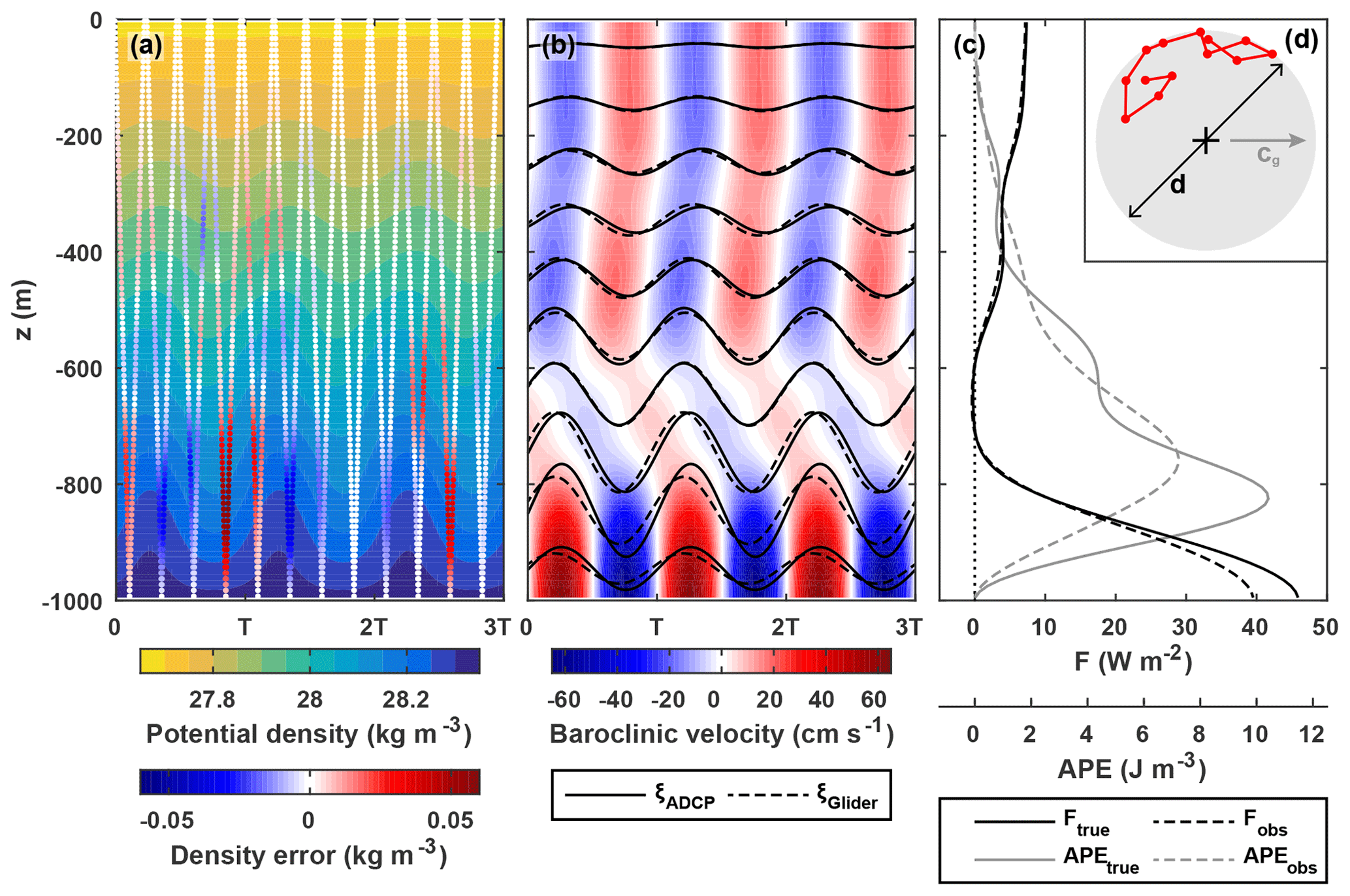
Figure 7 (a) Potential density for an idealized M₂ multi-mode internal tide overlaid with the error in measured density due to imperfect co-location of a glider and ADCP. The x axis is time in M₂ cycles. Positive error indicates an overestimation of density. (b) Baroclinic velocity (colour) for the same idealized internal tide overlaid with vertical isopycnal displacement at the ADCP (ξ_ADCP, solid black lines) and calculated from measured density (ξ_Glider, dashed black lines) every 100 m. (c) “True” and “observed” internal tide energy flux (black) and available potential energy (grey). (d) Location of the pseudorandomly distributed glider path (red) relative to the ADCP (black cross). The diameter of the watch circle, $d=\mathit{\lambda }/\mathrm{4}$, where λ=80 km is the mode-1 horizontal wavelength. c_g is the direction of tide propagation.

A single twelve-dive scenario for the $d=\mathit{\lambda }/\mathrm{4}$ case is shown in Fig. 7 to highlight the impact of mis-sampling density on observed energy flux and APE. This is an extreme example, with all the glider dives 6–10 km from the ADCP (Fig. 7d), and features near-bottom internal tide intensification similar to that observed on the northern flank of the WTR. In this example, the error in measured density is maximum in the lower half of the water column (where ξ_ADCP is up to 80 m; Fig. 7a, b); the resulting ξ_Glider underestimates ξ_ADCP by up to 20 m and leads by up to 40 min. Observed energy flux and APE underestimate true energy flux and APE over the majority of the water column (Fig. 7c); depth-integrated observed energy flux and APE underestimate depth-integrated true energy flux and APE by 772 W m⁻¹ (${\mathit{F}}_{\mathrm{err}}=-\mathrm{0.09}$) and 615 J m⁻² (${\mathrm{APE}}_{\mathrm{err}}=-\mathrm{0.2}$), respectively.

5.2 Energy flux error

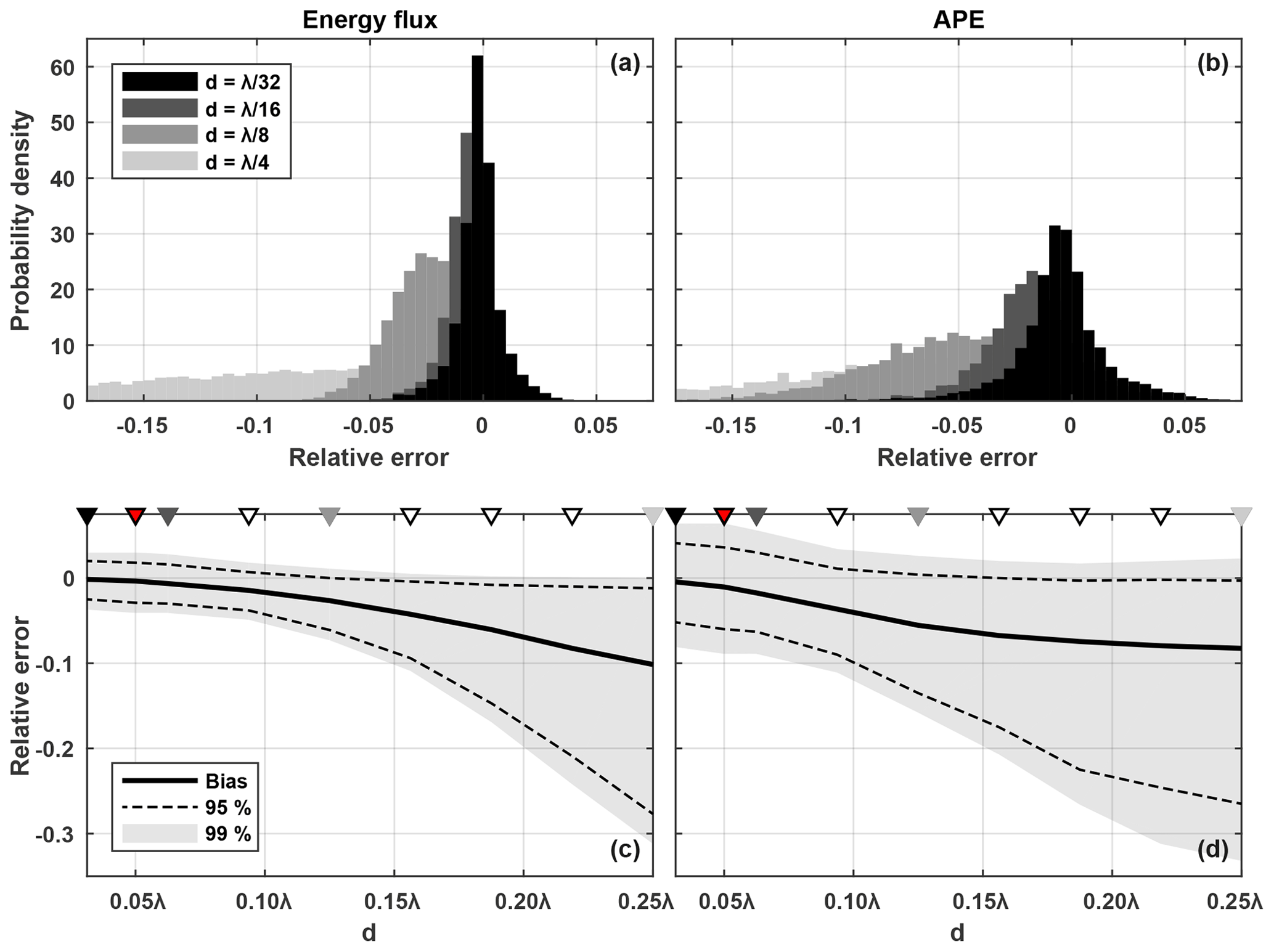
Figure 8 Histograms of (a) energy flux relative error and (b) APE relative error due to mis-sampling density in an idealized M₂ multi-mode internal tide field for the four watch circle diameter cases shown in Fig. 6. Positive error indicates an overestimation and negative error indicates an underestimation. Distribution of (a) energy flux relative error and (b) APE relative error against watch circle diameter, including the 99 % and 95 % confidence limits and the bias (median value). The four cases in panels (a) and (b) are indicated with black and grey triangles. The red triangle is the case most appropriate for the observations. The white triangles are four additional cases.

Histograms of F_err (0.005 wide bins) for four watch circle diameter cases are shown in Fig. 8a. The peaked distribution for the $d=\mathrm{1}/\mathrm{32}\mathit{\lambda }$ case broadens with increasing watch circle diameter as well as becoming biased towards negative error. The negative bias results from two related mechanisms. Firstly, the amplitude of ξ_Glider (and therefore $p_{\mathrm{Glider}}^{\prime }$) is typically underestimated for large watch circles because the glider samples density with a broad range of phase shifts, causing spectral smearing and poor harmonic fits to ξ. Secondly, maximum energy flux occurs when p^′ and ${\mathit{u}}_{\mathrm{bc}}^{\prime }$ are exactly in phase so any error in the phase of $p_{\mathrm{Glider}}^{\prime }$, positive or negative, will also result in a negative bias.

F_err distributions for all nine watch circle diameter cases are shown in Fig. 8c, including the 99 % and 95 % confidence limits and the bias (median value). As watch circle diameter increases, the width of the confidence intervals increases and the bias becomes progressively more negative. For the $d=\mathrm{1}/\mathrm{32}\mathit{\lambda }$ case, F_err is ±0.04 at the 99 % limit and the bias is near zero (−0.002). For the $d=\mathrm{1}/\mathrm{4}\mathit{\lambda }$ case at the other extreme, F_err is 0 to −0.31 at the 99 % limit and the bias is −0.1.

5.3 APE error

Histograms of APE_err for four watch circle diameter cases are shown in Fig. 8b. Compared with F_err, the distributions are broader and with a more negative bias for small watch circles. The broader distribution is explained by the error in ξ_Glider being squared in Eq. (9). The negative bias is explained by the first mechanism described in Sect. 5.2. APE_err distributions for all nine watch circle diameter cases are shown in Fig. 8d. Similar to F_err, the width of the confidence intervals increases and the bias becomes progressively more negative as watch circle diameter increases. For $d=\mathrm{1}/\mathrm{32}\mathit{\lambda }$, APE_err is ±0.08 at the 99 % limit and the bias is only −0.005. For $d=\mathrm{1}/\mathrm{4}\mathit{\lambda }$, APE_err is 0.02 to −0.33 at the 99 % limit and the bias is −0.08. Unlike F_err, the bias converges towards a constant value for very large watch circles.

6 Summary and discussion

Table 2 Distributions of energy flux relative error (F_err) and APE relative error (APE_err) for all nine watch circle diameter cases. d∕λ is watch circle diameter to mode-1 horizontal wavelength ratio. Positive error indicates an overestimation and negative error indicates an underestimation. The case most appropriate for the observations ($d/\mathit{\lambda }=\mathrm{0.05}$) is in bold.

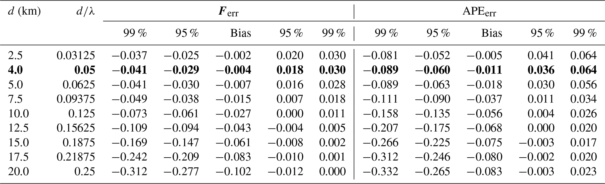
A novel approach to measuring internal tide energy flux using a co-located ocean glider and moored ADCP is tested using a dataset collected from the WTR in the North Atlantic. Gliders cannot perfectly hold station, even when operating as a virtual mooring, so error in the energy flux calculation due to imperfect co-location of the glider and ADCP is estimated by subsampling potential density in an idealized internal tide field along pseudorandomly distributed glider paths. If we consider the maximum acceptable energy flux error to be 0.1 (10 %), all the glider data must be contained within a watch circle with a diameter smaller than 1∕8 the mode-1 horizontal wavelength of the internal tide. Energy flux is biased low and the negative bias increases with increasing watch circle diameter. If watch circle diameter is larger than 1∕8 the mode-1 horizontal wavelength, the negative bias is more than −0.03 (3 %) and all realizations within the 95 % confidence interval are underestimates. When on-station over the WTR, the glider stayed within 2.5 km of the mooring so watch circle diameter d=5 km. The local D₂ mode-1 horizontal wavelength λ≈100 km so the $d/\mathit{\lambda }=\mathrm{0.05}$ case (Table 2) is the most appropriate for the observations presented here. The observed energy flux is estimated to have a negative bias of only −0.004 (0.4 %) and an error of less than ±0.03 (3 %) at the 95 % confidence limit. This estimate does not include the effect of internal tide advection by the barotropic tide (Stephenson et al., 2016), which can lead to an additional negative bias if barotropic velocity amplitude is of a similar size to baroclinic phase speed. Over the WTR, D₂ mode-1 phase speed is ≈2.2 m s⁻¹ and barotropic velocity amplitude is <0.2 m s⁻¹ so we expect this effect to be negligible for our observations.

At mid-latitudes, D₂ mode-1 horizontal wavelength for a 1000 m deep water column is typically in the range 40-160 km. The results presented here suggest energy flux error due to imperfect co-location can be reduced to an acceptable level (10 %) if the glider maintains a 5 to 20 km diameter watch circle. In the absence of strong tidal and slope currents, a well-trimmed glider diving to 1000 m with a relatively steep glide angle can usually maintain a watch circle with a diameter of 5 km or less, so energy flux error will typically be <10 %. Where horizontal wavelengths are shorter, for example at lower latitudes or in shallower and less stratified water columns, a smaller watch circle will be required to maintain an acceptable level of error. In shallower water, smaller watch circles are generally achievable because horizontal travel over a complete dive cycle scales with dive depth. Diurnal internal tides have longer horizontal wavelengths so larger watch circles are acceptable. For mission planning, the mode-1 horizontal wavelength of a tidal frequency ω can be estimated, $\mathit{\lambda }=\mathrm{2}\mathit{\pi }{c}_{\mathrm{1}}/\sqrt{{\mathit{\omega }}^{\mathrm{2}}-f^{\mathrm{2}}}$, where f is the inertial frequency and $c_{\mathrm{1}}=NH/\mathit{\pi }$ is an approximation of mode-1 eigenspeed. If the assumption of uniform stratification is not appropriate, c₁ can be calculated by solving the boundary value problem for a given N(z) (Gill, 1982). Table 2 can then be used to estimate the energy flux bias and error that can be expected for a given value of d∕λ.

Including the above estimate of error due to imperfect co-location, the observed depth-integrated D₂ internal tide energy flux over the northern flank of the WTR is 4.2±0.2 kW m⁻¹. This is considerably larger than previous internal tide observations over the southeastern bank of the FSC: 0.2 kW m⁻¹ (90 km northeast of the WTR; Hall et al., 2011) and 0.4–0.6 kW m⁻¹ (105 km northeast of the WTR; Hall et al., 2017b), but small compared with some deep-ocean ridges, e.g. the Hawaiian Ridge (up to 33 kW m⁻¹; Lee et al., 2006) and Luzon Strait (up to 41 kW m⁻¹; Alford et al., 2011). More comparable to the WTR is the Mendocino Escarpment, where a ridge is orientated perpendicular to the continental slope and the observed energy flux is 7 kW m⁻¹ (Althaus et al., 2003).

The 40 h co-located time series presented here is not long enough to resolve the internal spring–neap cycle. Peak neap tide occurred on yearday 153², 1 day before the majority of the co-located time series. Assuming the internal tide is generated locally at the WTR, the surface and internal spring–neap cycles will be in phase. The observed D₂ energy flux is therefore representative of neap internal tide and so an underestimate of the true M₂ internal tide. This may somewhat explain the slight underestimate compared to the M₂-only regional tide model. Interestingly, the CTD time series used by Sherwin (1991) was recorded 2 days after peak spring tide so is more representative of spring internal tide. The fact that two observational estimates of D₂ vertical isopycnal displacement, 6.7 km apart and at different phases of the internal spring–neap cycle, are so similar implies that there are compensating spatial gradients in internal tide magnitude. The regional tide model shows the possible extent of these gradients and suggests that accurate siting of moorings is crucial for repeated long-term observations.

For future experiments, spatial gaps in the time series can be minimized with conductivity–temperature loggers and additional current meters on the mooring line. We have also shown that glider-inferred DAC can provide an accurate estimate of tidal current velocity that could be used to constrain barotropic velocity in the absence of full-depth data coverage by ADCPs and current meters. However, the major limitation of the dataset presented here is the short length of the co-located time series. Future glider missions will hold station by an ADCP mooring for several weeks to resolve the internal spring–neap cycle. Calculating D₂ internal tide energetics in a 36 h moving window will yield a time-varying energy flux that can be related to seasonal changes in stratification, advection by mesoscale eddies, spatial and temporal patterns in internal tide-driven turbulent mixing, and the resulting biogeochemical response.

Appendix A: Idealized internal tide field

An idealized M₂ multi-mode internal tide field is created for a 1000 m deep water column with uniform stratification ($N^{\mathrm{2}}=\mathrm{6.1}\times {\mathrm{10}}^{-\mathrm{6}}$ s⁻²). Horizontal current velocity, $\mathit{u}=(u,v)$, and vertical isopycnal displacement, ξ, are defined by summing the first 10 baroclinic modes,

$$\begin{array}{}\text{(A1)}& \begin{array}{rl}& u(x,y,z,t)=\sum _{n=\mathrm{1}}^{\mathrm{10}}{u}_n\sin (k_{n}x-\mathit{\omega }t-{\mathit{\varphi }}_n)A_n\left(z\right),\\ & v(x,y,z,t)=\sum _{n=\mathrm{1}}^{\mathrm{10}}{u}_n{\displaystyle \frac{f}{\mathit{\omega }}}\cos (k_{n}x-\mathit{\omega }t-{\mathit{\varphi }}_n)A_n\left(z\right),\end{array}\end{array}$$

and

$$\begin{array}{}\text{(A2)}& \begin{array}{rl}& \mathit{\xi }(x,y,z,t)=\\ & \sum _{n=\mathrm{1}}^{\mathrm{10}}{u}_n\sin (k_{n}x-\mathit{\omega }t-{\mathit{\varphi }}_n)B_n\left(z\right){\displaystyle \frac{\mathrm{1}}{\mathit{\omega }}}{\left({\displaystyle \frac{{\mathit{\omega }}^{\mathrm{2}}-f^{\mathrm{2}}}{N^{\mathrm{2}}-{\mathit{\omega }}^{\mathrm{2}}}}\right)}^{\mathrm{1}/\mathrm{2}},\end{array}\end{array}$$

where u_n and ϕ_n are the velocity amplitude and the phase of the nth baroclinic mode, respectively; $\mathit{\omega }=\mathrm{1.41}\times {\mathrm{10}}^{-\mathrm{4}}$ s⁻¹ is the M₂ frequency; and $f=\mathrm{1.26}\times {\mathrm{10}}^{-\mathrm{4}}$ s⁻¹ is the inertial frequency at 60^∘ N. A_n(z) and B_n(z) are the vertical structures of horizontal current velocity and vertical isopycnal displacement for each baroclinic mode, and are equivalent to cos (nπz∕H) and sin (nπz∕H), respectively, where n is mode number. Horizontal wavenumber $k_n=\sqrt{{\mathit{\omega }}^{\mathrm{2}}-f^{\mathrm{2}}}/c_n$, where $c_n=NH/n\mathit{\pi }$, is an approximation of mode eigenspeed (Gill, 1982). Velocity amplitude decays with mode number, $u_n=u_{\mathrm{1}}{e}^{-\mathrm{0.5}(n-\mathrm{1})}$, where u₁ is the mode-1 velocity amplitude. This decay rate results in a well-defined internal tide beam if velocity phase is approximately equal for each baroclinic mode. However, a different random set of baroclinic mode phases (ϕ_n) is used for each scenario simulated so internal tide beams are only apparent in a subset of scenarios. u₁=0.28 m s⁻¹ yields a mode-1 vertical isopycnal displacement amplitude of 50 m but energy flux error and APE error are not sensitive to absolute amplitude. The time-varying potential density field is then

$$\begin{array}{}\text{(A3)}& \mathit{\rho }(x,y,z,t)=\stackrel{\mathrm{‾}}{\mathit{\rho }}\left(z\right)+{\displaystyle \frac{{\mathit{\rho }}_{\mathrm{0}}}{g}}{N}^{\mathrm{2}}\mathit{\xi },\end{array}$$

where $\stackrel{\mathrm{‾}}{\mathit{\rho }}\left(z\right)$ is a background density profile with a vertical gradient equivalent to N². Barotropic velocity (${\mathit{u}}_{\mathrm{bt}}^{\prime }$) and residual flow ($\stackrel{\mathrm{‾}}{\mathit{u}}$) are both zero so ${\mathit{u}}_{\mathrm{bc}}^{\prime }=\mathit{u}$.