the Creative Commons Attribution 3.0 License.
the Creative Commons Attribution 3.0 License.
Reconstruction of sea level around the Korean Peninsula using cyclostationary empirical orthogonal functions
Se-Hyeon Cheon
Benjamin D. Hamlington
Kyung-Duck Suh
Since the advent of the modern satellite altimeter era, the understanding of the sea level has increased dramatically. The satellite altimeter record, however, dates back only to the 1990s. The tide gauge record, on the other hand, extends through the 20th century but with poor spatial coverage when compared to the satellites. Many studies have been conducted to create a dataset with the spatial coverage of the satellite datasets and the temporal length of the tide gauge records by finding novel ways to combine the satellite data and tide gauge data in what is known as sea level reconstruction. However, most of the reconstructions of sea level were conducted on a global scale, leading to reduced accuracy on regional levels, especially when there are relatively few tide gauges. The seas around the Korean Peninsula are one such area with few tide gauges before 1960. In this study, new methods are proposed to reconstruct past sea level around the Korean Peninsula. Using spatial patterns obtained from a cyclostationary empirical orthogonal function decomposition of satellite data, we reconstruct sea level over the period from 1900 to 2014. Sea surface temperature data and altimeter data are used simultaneously in the reconstruction process, leading to an elimination of reliance on tide gauge data. Although we did not use the tide gauge data in the reconstruction process, the reconstructed sea level has a better agreement with the tide gauge observations in the region than previous studies that incorporated the tide gauge data. This study demonstrates a reconstruction technique that can potentially be used at regional levels, with particular emphasis on areas with poor tide gauge coverage.
- Article
(5673 KB) - Full-text XML
- BibTeX
- EndNote


Although sea level rise is a global phenomenon, the impacts are different in localities. Changes in sea level are affecting communities across the globe on an almost daily basis through increased erosion, greater saltwater intrusion, more frequent nuisance flooding, and higher storm surges causing severe damage on coastal structures (Cheon and Suh, 2016; Nicholls, 2011; Suh et al., 2013). Planning for, adapting to, and mitigating current and future sea level has necessarily begun in many threatened areas. Important decisions have been made in both economic and societal activities. Examples can be found throughout the world, with coastal communities making difficult decisions on how to address concerns associated with future sea level rise (Nicholls, 2011). The present and near-term threat of sea level rise across the globe highlights the immediate need for actionable regional sea level projections. In order to improve future projections of sea level, understanding past sea level change is an important first step.
Before the satellite altimeter era, the only available sea level observations came from tide gauge (TG, hereafter) records. TGs provide records of local sea level variations, covering nearly 200 years in some locations around the globe. Using TG data, scientists have studied past sea level changes around the world. However, TGs provide poor spatial coverage as they are located at coastal sites and mostly in the Northern Hemisphere. On the other hand, the satellite altimeters collecting data since 1992 have near-global coverage of sea level but a relatively short observation period compared to TG observations, which is a severe handicap to analyzing long-term changes in sea level. This disadvantage is particularly true given the presence of sea level variability with decadal and longer timescales.
Chambers et al. (2002) was one of the first to reconstruct sea level anomalies (SLAs) by combining TG data and satellite altimeter data. In their research, they studied low-frequency variability in global mean sea level (GMSL) from 1950 to 2000. They interpolated sparse TG data into a global gridded SLA pattern applying EOFs (empirical orthogonal functions) of SLA using data from the TOPEX/Poseidon satellite altimeter to capture the interannual-scale signals, e.g., ENSO (El Niño–Southern Oscillation) and PDO (Pacific Decadal Oscillation). Building on previous studies (Chambers et al., 2002; Kaplan et al., 1998, 2000), Church et al. (2004) created a reconstruction from 1950 to 2001 using EOFs of SLA data measured from satellite altimeters and a reduced-space optimal interpolation scheme. This research was subsequently updated to increase temporal coverage from 1870 to the present (Church and White, 2006, 2011), and the reconstructions have been made available to the public through their website (https://research.csiro.au/slrwavescoast/sea-level/measurements-and-data/sea-level-data/; last access: 1 January 2018). In these studies, GMSL was found to rise approximately 210 mm from 1880 to 2009, with a linear trend from 1900 to 2009 of 1.7 ± 0.2 mm yr−1. The resulting SLA is one of the most comprehensive and widely cited reconstructions. While these studies focused largely on the reconstruction of GMSL, Hamlington et al. (2011) applied cyclostationary empirical orthogonal functions (CSEOFs) as basis functions for the reconstruction of SLA in an attempt to improve the representation of variability about the long-term trends. This approach provided an advantage for describing local variations such as ENSO and PDO. After that, Hamlington et al. (2012a) proposed an improved scheme of their reconstruction using sea surface temperature (hereafter SST). Given the limited TG data in the past, reconstruction of SLA relying only on TGs was inaccurate, particularly before 1950. Leveraging other ocean observations (e.g., SST) led to an improved SLA reconstruction further into the past. In addition, this approach provides an advantage for describing local variations such as ENSO and PDO because the SST data give information where only few TGs are available.
While sea level is a global phenomenon, the extent of sea level change varies dramatically across the globe. During the 24-year satellite altimeter record, regional trends have been measured to be 4 times greater than the global average in some areas (AVISO, 2017). Therefore, sea level assessment on a regional level is necessary to plan for future sea level. Several studies have focused on regional reconstructions targeting a particular area of interest. As an example, using an optimal interpolation method, Calafat and Gomis (2009) reconstructed the distribution of SLA in the Mediterranean Sea over 1945–2000. They used EOFs of satellite altimeter data spanning from 1993 to 2005 as basis functions and interpolated the TG data using these spatial patterns. A spatial distribution of sea level rise trends for the Mediterranean for the period of 1945–2000 indicated a positive trend in most areas. Hamlington et al. (2012b) performed a regional SLA reconstruction using CSEOFs as basis functions (Hamlington et al., 2011) with a domain covering only the Pacific Ocean. They found that a choice of basis functions had a significant effect on the spatial pattern of the sea level rise and the ability to capture internal variability signals. Global basis functions, either CSEOFs or EOFs, are typically dominated by large-scale variability in the Pacific Ocean associated with ENSO or the PDO. As a result, global reconstructions are poorer in some ocean basins (e.g., Indian Ocean, Atlantic Ocean) than others (Pacific Ocean). This issue is likely exacerbated further when looking at even smaller regions.
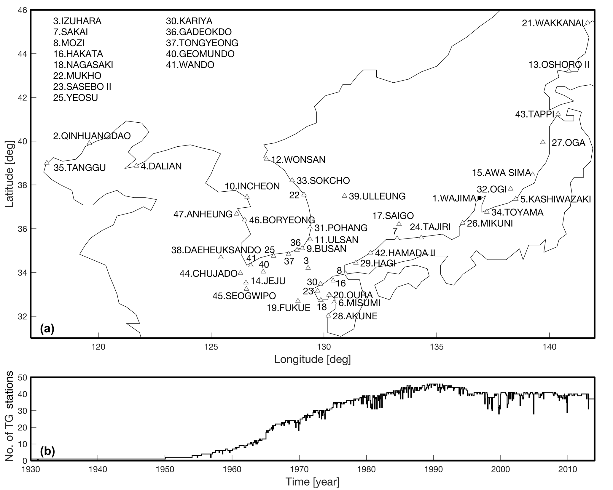
Figure 1(a) The locations of tide gauge station used in this study around the Korean Peninsula. The black square is Wajima station which has the longest record length (1930–present); (b) the number of tide gauge stations provided by the Permanent Service for Mean Sea Level (PSMSL) around the Korean Peninsula.
In this paper, we focus on one such region: the seas around the Korean Peninsula. In South Korea, over 27 % of its 45 million people live in coastal city areas, and nearly 36 % of gross regional domestic product is produced by coastal city regions (Choi and Jeong, 2015). As a result, policymakers have a keen interest in a sea level rise around the Korean Peninsula (hereafter KP; a suffix, “-KP”, means the spatial domain of the data or variable is around the Korean Peninsula) to establish proper remedies to sea level rise. Studying SLA-KP, researchers have primarily relied upon globally reconstructed SLAs (Church and White, 2011; Hamlington et al., 2011). However, extracting SLA-KP (or more generally for any small region) from a globally reconstructed SLA has some problems. First, global-scale reconstructions use a limited number of basis functions to prevent the interpolation from overfitting and creating spurious sea level fluctuations. There is a difference between the dominant modes of variability at the global scale and local scale; e.g., there is a high possibility that the globally selected basis functions, which represent 90 % of the total variance in the global level, will not represent 90 % of the total variance in local scale. Second, the coverage of the TG around the KP (TG-KP) started around 1930 and only one TG was available until 1950; it is too little to secure accuracy on these local scales. As mentioned above, TG-KP coverage is poor extending back into the 20th century, and relatively few TGs are available to analyze in some areas (Fig. 1). Hence, the goal of this study is to propose a new scheme that builds on Hamlington et al. (2012b) that applies CSEOFs to reconstruct local SLA where the TG data are not enough to ensure a quality reconstruction through the 20th century. We focus on the KP both due to its exposure to risk from impending sea level rise and also as a test case to demonstrate how this technique could be applied at other locations across the globe.
2.1 Data
2.1.1 Sea level anomalies
The basis functions of this study's reconstructions are the CSEOFs of gridded satellite data of SLA provided by AVISO (the Archiving, Validation, and Interpretation of Satellite Oceanographic data; https://www.aviso.altimetry.fr/en/data/products/sea-surface-height-products/global/msla-mean-climatology.html; last access: 1 March 2017) from 1993 to 2015. These monthly data have a resolution, and hereafter this dataset is written as AVISO. Before conducting the CSEOF decomposition, mean values for each grid point were removed. The annual signal has not been removed as it is accounted for by the CSEOF analysis (see more details in Sect. 2.2.1). The data were trimmed to contain only the seas around the KP (31–46∘ N and 117–142∘ E), and they were multiplied by the square root of the cosine of latitude to consider the actual area of each grid.
2.1.2 Sea surface temperature
In this study, two SST reconstruction datasets were used: ERSST (Huang et al., 2015, 2016; Liu et al., 2015) and COBESST2 (Ishii et al., 2005). The ERSST is a global monthly SST dataset that was reconstructed based on the observation of ICOADS (International Comprehensive Ocean-Atmosphere Dataset). This monthly analysis has a grid resolution and its time coverage is from 1854 to the present, and the included data are anomalies based on a monthly climatology computed from 1971 to 2000. The COBESST2 dataset is a monthly interpolated SST product from 1850 to the present. It integrates several SST observations: ICOADS 2.5, satellite SST, and satellite sea ice. In addition to the OI (optimal interpolation) scheme, this dataset used an EOF reconstruction.
Each dataset was trimmed to three different regions: a global domain (no trim), the northwest Pacific domain (25–55∘ N and 110–160∘ E), and around the KP area. Before conducting the CSEOF decomposition, these datasets were treated as follows. (1) The mean values for each grid point were removed. (2) The data were weighted by the square root of the cosine of latitude to consider the actual area of each grid. (3) Any grid points that were not continuous in time were removed. Like the satellite altimeter dataset, an annual signal was not removed.
2.1.3 Tide gauge data
Monthly mean records of 47 TGs were obtained from the Permanent Service for Mean Sea Level (PSMSL, Fig. 1) from 1930 to 2013. The earliest data of the TGs are traced back to 1930 at Wajima station (Fig. 1). Before 1965, the number of available TG records is fewer than 10, with only one TG (Wajima station) providing data until 1950. An ongoing GIA (glacial isostatic adjustment) correction was applied to the TG data using ICE-5G VM2 model (Peltier, 2004). Since an IB (inverted barometer) correction was applied to the satellite altimetry data, the TG data are IB corrected based on the pressure fields from 20th century reanalysis V2c data (Compo et al., 2006, 2011; Hirahara et al., 2014). The TG data in this study are modified with further editing criteria. The techniques for editing are similar to those of Hamlington et al. (2011), with TGs that have shorter record length than 5 years and unphysical trends (greater than 7 mm yr−1, likely due to uncorrectable vertical land motions) being removed prior to analysis. After calculating a month-to-month change, jumps greater than 250 mm were also removed.
2.1.4 Reconstructed sea level anomalies of previous studies
Church and White (2006, 2011) created the reconstruction of a global SLA from 1870 to 2009 using EOFs of SLA from satellite altimetery over 1993–2009, and the resulting SLA is one of the most comprehensive and widely cited reconstruction results. The Church and White (2006, 2011) dataset was employed for the long-term background trend for this study (see Sect. 2.2.3). The GMSL time series (Church and White, 2006, 2011) has been extended and made publicly available (https://research.csiro.au/slrwavescoast/sea-level/measurements-and-data/sea-level-data/; last access: 1 January 2018). To reconstruct the past SLA, Hamlington et al. (2011) combined the CSEOFs of the satellite altimetry and historical TG record. This weekly analysis has a grid resolution and its time coverage is over 1950–2009. This dataset was used for the comparison with the reconstruction of this study (see Sect. 2.2.3). This reconstruction dataset (Hamlington et al., 2011) can be downloaded from the NASA JPL/PO.DAAC (ftp://podaac.jpl.nasa.gov/allData/recon_sea_level/preview/L4/tg_recon_sea_level/; last access: 1 March 2017).
2.2 Methods
We propose a modified reconstruction method for the seas around the Korean Peninsula which have poor TG coverage. This method is a progression from the technique described in Hamlington et al. (2012a). Previous studies (Church and White, 2006, 2011; Church et al., 2004; Hamlington et al., 2011, 2012a) decomposed SLA into spatial patterns and corresponding amplitude time series, and extended the time series back in time, assuming similar spatial patterns over the full record. We decompose SLA-KP using CSEOF analysis and extend amplitude time series using SST data applying multivariate regression that accounts for time lags. In this section, we detail the procedure and discuss the underlying theory.
2.2.1 Cyclostationary empirical orthogonal functions
To understand the complex response of a physical system, the decomposition of data into a set of basis functions is frequently applied. The decomposed basis functions have the potential to give a better understanding of complex variability of the fundamental phenomenon. The simplest and most common computational basis functions are EOFs, which have often served as the basis for climate reconstructions. When a reconstruction selects the EOFs as basis functions, one basis function is defined as a single spatial map accompanied by a time series representing the amplitude modulation of this spatial pattern over time. The EOF decomposition of the spatiotemporal system, T(r,t), is defined by Eq. (1):
where LV(r) (loading vector) is a physical process modulated by a time series PCT(t) (principal component time series or PC time series). Combining each LV and PCT pair, a signal of single EOF mode can be produced.
The assumption underlying EOF-based reconstruction is the stationarity of the spatial pattern represented by the EOF over the entire period. However, the fact that many geophysical phenomena are cyclostationary is well known (Kim et al., 2015). That is, some processes are periodic over a certain inherent timescale, with corresponding amplitudes varying over time. Even though EOFs represent cyclostationary signals through a superposition of multiple modes, as stated in Dommenget and Latif (2002), representing the cyclostationary signals with stationary EOFs can lead to an erroneous and ambiguous interpretation of the data. It also requires many EOFs to explain a relatively small amount of variability in a dataset.
To remedy some of these issues, Hamlington et al. (2011) introduced CSEOFs as the basis for the global reconstruction of SLA instead of EOFs. The CSEOF analysis proposed to capture the cyclostationary patterns and longer-scale fluctuations in geophysical data (Kim and Chung, 2001; Kim and North, 1997; Kim and Wu, 1999; Kim et al., 1996, 2015). The CSEOF analysis can capture the time-varying signals as a single mode by giving a time dependency to the loading vectors.
The system is defined as Eqs. (2) and (3):
where CSLV(r,t) is a cyclostationary loading vector (for convenience, we call this LV) and it is time dependent and periodic with a particular period d (called a “nested period”). Previous studies (Kim and North, 1997; Kim et al., 1996, 2015) provide more detailed walk-through for the CSEOF computation and properties. CSEOFs have a significant advantage over EOFs since CSEOFs can explain cyclostationary signals in one mode; that is, CSEOFs of periodic processes are much easier to interpret than EOFs (Kim and North, 1997; Kim and Wu, 1999; Kim et al., 1996, 2015). Hamlington et al. (2011, 2012a, b) demonstrated that CSEOFs provided significant benefits dealing with repeating signals such as ENSO and modulated annual cycle signals.
2.2.2 Multivariate regression using CSEOFs
When considering the complete Earth climate system, one variable is often directly connected to another variable. In some cases, they are impacted by a common physical process, or in other cases, one variable may directly influence another. To take advantage of these relationships and establish links, we can perform a multivariate linear regression such as Eq. (4).
where β0, β1, β2, ⋯, and βk are regression coefficients, and ϵ is random error. In this study, the response variables are each PCT of AVISO's CSEOF and the predictor variables are all PCTs of each SST dataset's CSEOF. Equation (4) can be rewritten as follows:
where PCT is the nth component of the mth PCT of AVISO's CSEOF, PCT is the nth component of the kth PCT of SST's CSEOF, and are regression coefficients for the mth target and kth PCT of SST (, , …, M, and , …, N; K, M, and N are the total numbers of predictors, targets, and time steps, respectively). The matrix form of Eq. (5) is
where and are PCT and PCT, respectively.
Additionally, many geophysical signals have lagged relations with other geophysical signals (Bojariu and Gimeno, 2003; Dettinger et al., 1998; Hamlet et al., 2005; Hendon et al., 2007; Kawamura et al., 2004; McPhaden et al., 2006; Redmond and Koch, 1991). Hence, by assuming that each mode of CSEOF represents an independent physical event, we can assume the PCTs which are mathematically independent of each other also can have a lagged relationship. If we consider the lagged relationships between the target and predictor variables and use only the predictors having a higher correlation, we can reduce the number of predictors in the regression; generally, the more predictors applied for the regression, the more noise is likely to appear in the result. Before performing the multivariate linear regression as in Eq. (5), we calculated the cross-correlation between the target PCT of AVISO and predictor PCTs of SST. The predictors were selected based on their cross-correlation values. The threshold cross-correlation value did not have a significant effect on the regression as long as the value was chosen to allow for at least 10 predictors; in this study, we used 0.3 as the threshold. By assuming the lag of the ith mode with the mth target having maximum cross-correlation at , the mth mode's PCT of AVISO can be given as follows based on Eq. (5):
where PCT is the nth component of the mth PCT of AVISO's CSEOF, and PCT is the nth component of the ith PCT of SST's CSEOF; is a lag of maximum correlation between the ith predictor and the mth target; and represent regression constants and regression coefficients for the mth target.
To use Eq. (7), we need time lags of the maximum correlation () and the results of CSEOF decomposition of SLA-KP and SST for the same period (PCT and PCT); by Eq. (7), we can estimate the regression coefficients ( and ). Using the regression coefficients and SST's PCTs which cover the past, we can extend SLA's PCTs prior to the altimeter record.
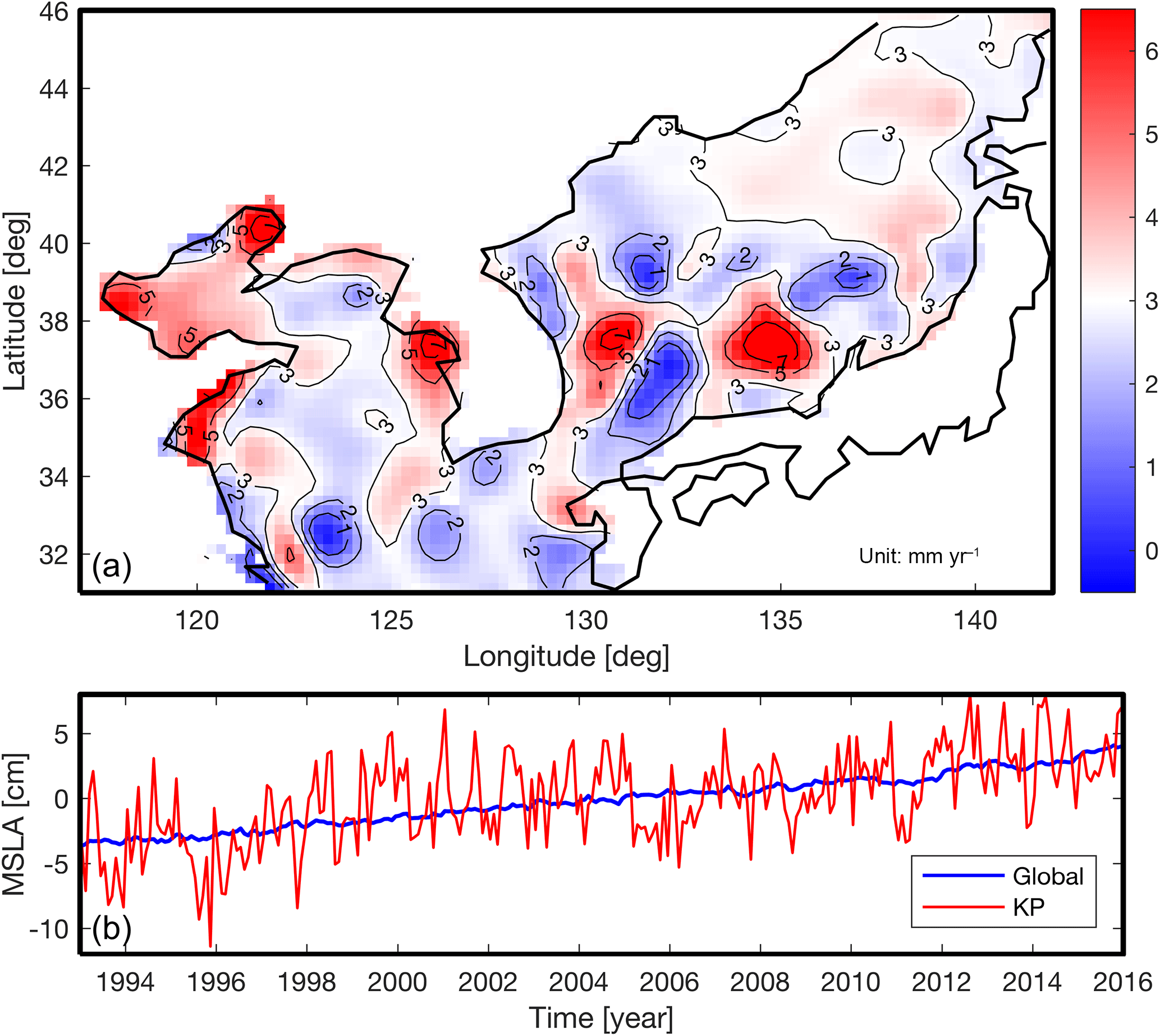
Figure 2(a) Linear trend map of sea level anomalies around the Korean Peninsula from AVISO without annual signal from 1993 to 2015 (the red-colored area has a higher linear trend than 3.0 mm yr−1, and the blue-colored area has a lower linear trend than 3.0 mm yr−1); (b) spatial mean time series of sea level anomalies around the Korean Peninsula (red) and global (blue) from AVISO without annual signal.
2.2.3 Reconstruction of sea level anomalies
As a starting point, AVISO was trimmed around the KP and the southeast sea of the Japanese islands was removed. GMSL and mean values were removed from AVISO at each grid point. Each SST dataset was trimmed to have the time span of 1891–2014 and cut into three regions: around the KP, the northwest Pacific Ocean, and global (no trimming). In total, we made six different SST combinations (ERSST and COBESST2 for three regions). All grid points that were not continuous in time were removed for every dataset. Each data point was weighted by the square root of the cosine of latitude to consider the actual area of each grid. We conducted the CSEOF decomposition for all data (AVISO without GMSL over 1993–2014 and six SST combinations over 1891–2014) with a 12-month nested period because an annual signal is the most robust repeating signal of SLA. The lagged relation between PCTs of AVISO and SST datasets were estimated with 2 years maximum lag. Using the PCTs of each dataset's CSEOF, we built the multiple linear regressions based on Eq. (7) over 1993–2014. In this regression, the target variables were each PCT of AVISO and the predictors are PCTs of each SST combination; the regression coefficients and their confidence intervals were estimated. Applying a Monte Carlo simulation that used the confidence intervals of regression coefficients, we randomly generated a thousand sample sets of the regression coefficients; by substituting the regression coefficient sets and PCTs of SSTs over 1891–2014 into Eq. (7), we reproduced a thousand sets of PCTs of AVISO from 1891 to 2014. By combining the extended PCTs to the LVs of AVISO, we produced a thousand SLAs without GMSL. By adding randomly generated GMSLs (Church and White, 2011) to the reconstructed SLAs, a thousand SLAs were generated. Finally, by statistical analysis of each time step of the random samples, we estimated the mean variation and their confidence intervals of each reconstruction.
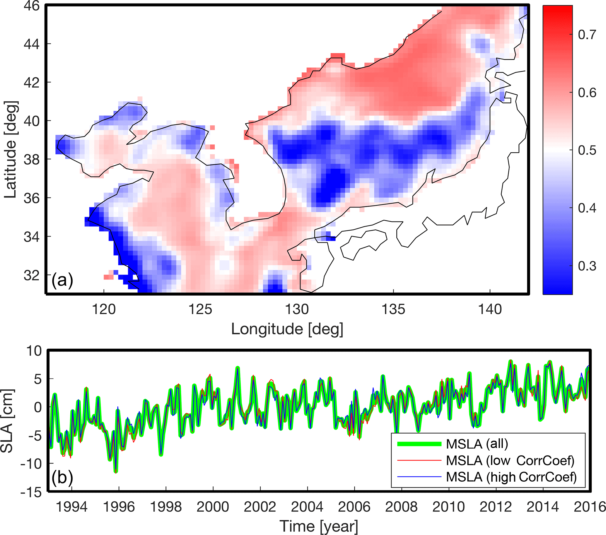
Figure 3(a) Mean correlation coefficient map of sea level anomalies around the Korean Peninsula from AVISO without annual signal from 1993 to 2015; (b) spatial mean time series of sea level anomalies from two regions of panel (a) where the red-colored area is the high-correlation coefficient zone and the blue-colored area is the low-correlation coefficient zone.
For comparison, in addition to the TG, we used the reconstructed dataset of Hamlington et al. (2011). We trimmed the dataset to have same domain as this study. The reconstruction results over 1970–2009 are quite reliable, because, after 1970, the number of available TG records around the world is enough to accurately represent sea level in the reconstruction. The correlation coefficient (ρ) and NRMSE (normalized root mean square error; we obtain this value through dividing RMSE by the standard deviation of the reference dataset; Eq. 8) values for the entire domain and each TG location were calculated. By using these two values, we decided the best reconstruction case among the six reconstructions which are introduced in Sect. 3.2.
where indicates the Euclidean norm (or 2-norm) of a vector, xref and x are reference data and tested data, respectively.
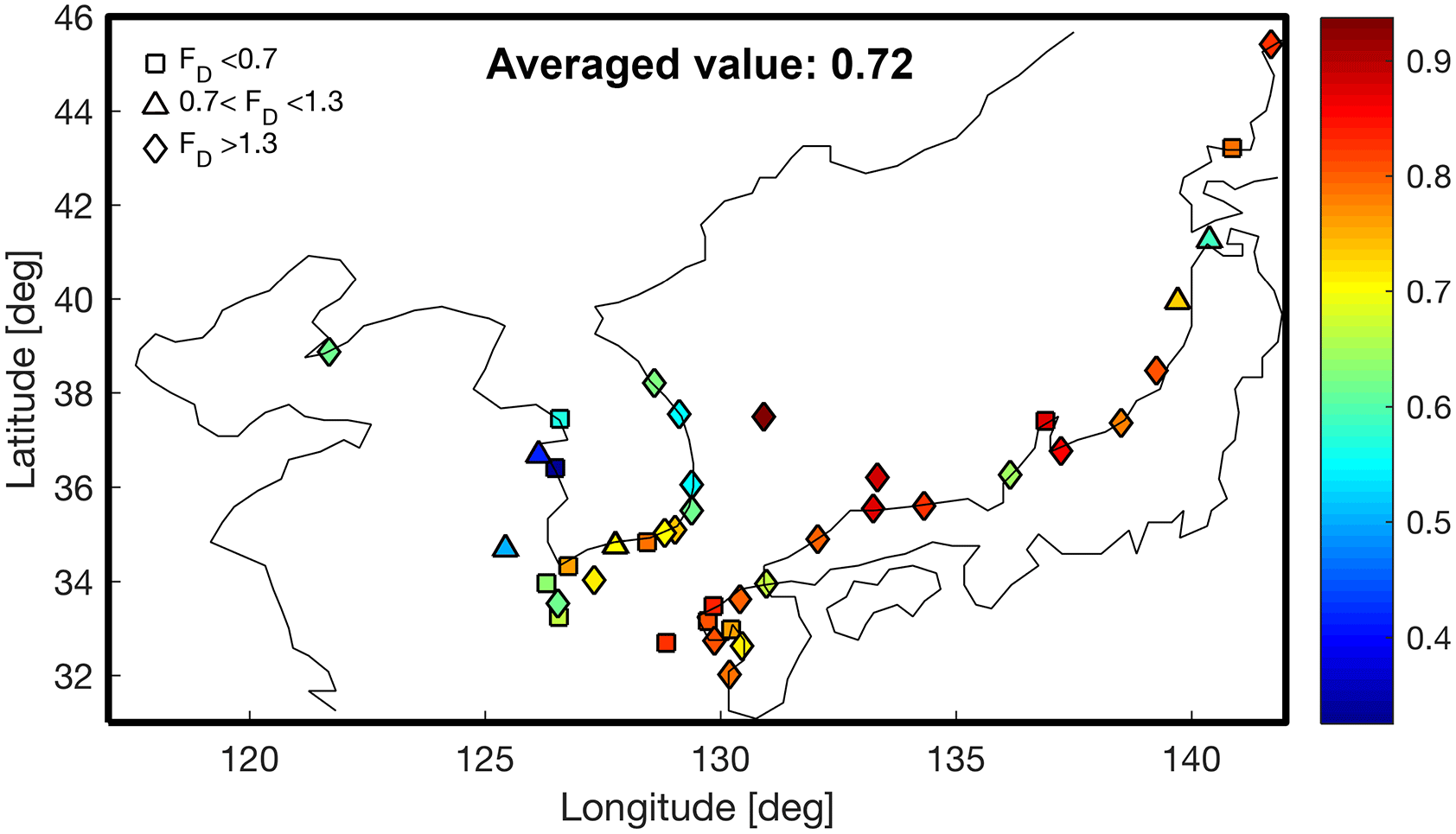
Figure 4Linear trends comparison (shapes) and correlation coefficients (colors) between tide gauge and the closest AVISO grid point (< 12 km) from 1993 to 2014, where (without annual signals).
3.1 Sea level anomalies around the Korean Peninsula
Using AVISO over 1993–2015, a linear trend map was estimated as shown in Fig. 2. The mean trend was found to be 3.1 ± 0.5 mm yr−1. The linear trend of mean SLA-KP agrees closely with the GMSL trend, 3.0 ± 0.4 mm yr−1 (Fig. 2). Due to the similarity between the long-term trends of mean SLA-KP and GMSL (Fig. 2), it is reasonable to assume that the SLA-KP can be described as the combination between background signals (GMSL) and the residuals which contain local characteristics of SLA-KP. Most of the SLA-KP trends were close to the mean, but some parts of the East Sea/Sea of Japan, and of the Yellow Sea close to land exhibited extreme patterns. Some areas showed trends over 7 mm yr−1, while in other regions the linear trends were less than 1 mm yr−1 (Fig. 2). To check whether the extreme linear trend patterns had a significant influence on mean SLA-KP, we compared the mean SLA of the area having the extreme linear trends and the other area. We calculated the mean correlation (hereafter ) of each grid point of AVISO to separate the two areas. For example, at a single grid point P was calculated by taking mean of ρ values that had been estimated between P and all other points. By repeating these calculations at all the points of AVISO, we obtained Fig. 3. We thought that the SLAs of the regions having relatively high fluctuate together; on the other hand, the SLAs of the low regions oscillate separately. The regions that had the relatively low correlation coefficient agreed with the regions that had the extreme linear trends (Figs. 2 and 3). We divided the SLA-KP into two regions according to the mean correlation coefficient; we roughly selected the threshold value as 0.5, which can separate the area having extreme trends and the remaining area. The mean SLAs of the two regions agree well with each other (Fig. 3). This demonstrates that the small-scale extreme features tend to cancel out and do not significantly impact mean SLA-KP. This also suggests that the entire region can be treated as local variability fluctuating about some background long-term mean, an important feature for this reconstruction procedure.
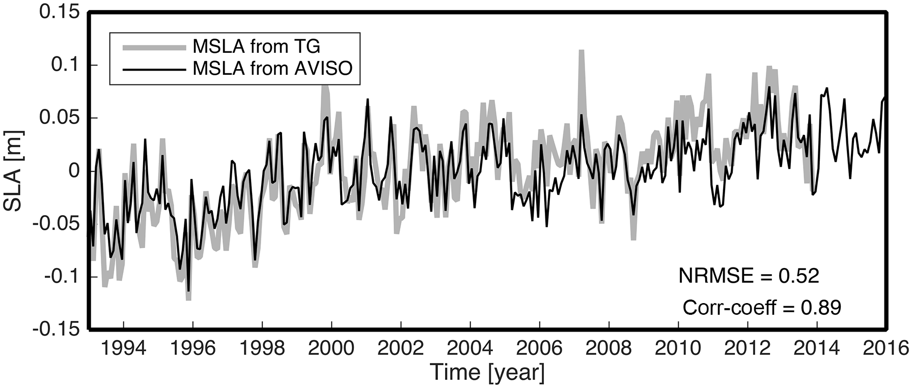
Figure 5Spatial mean time series of sea level anomalies of tide gauge and AVISO around the Korean Peninsula without annual signal.
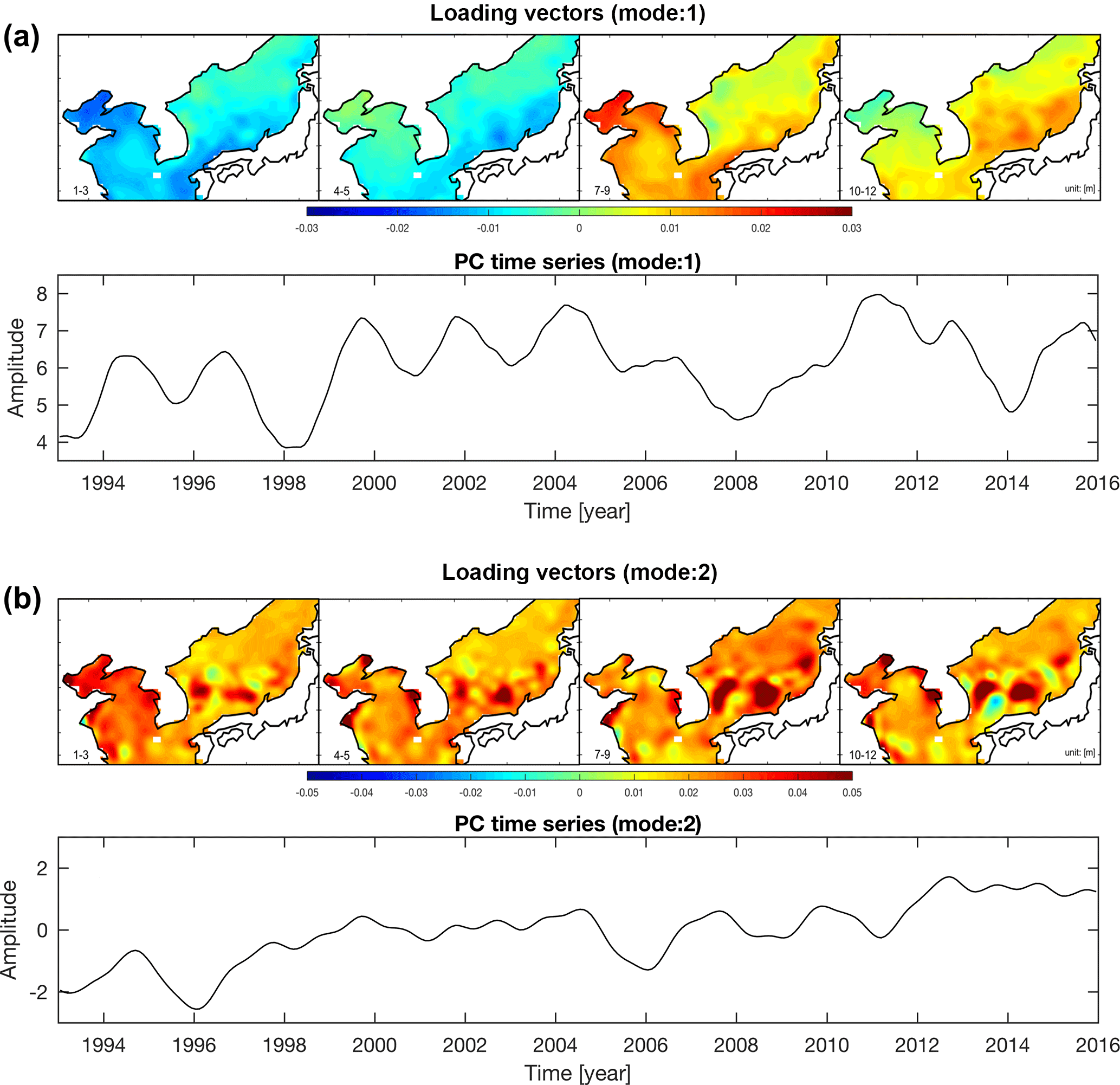
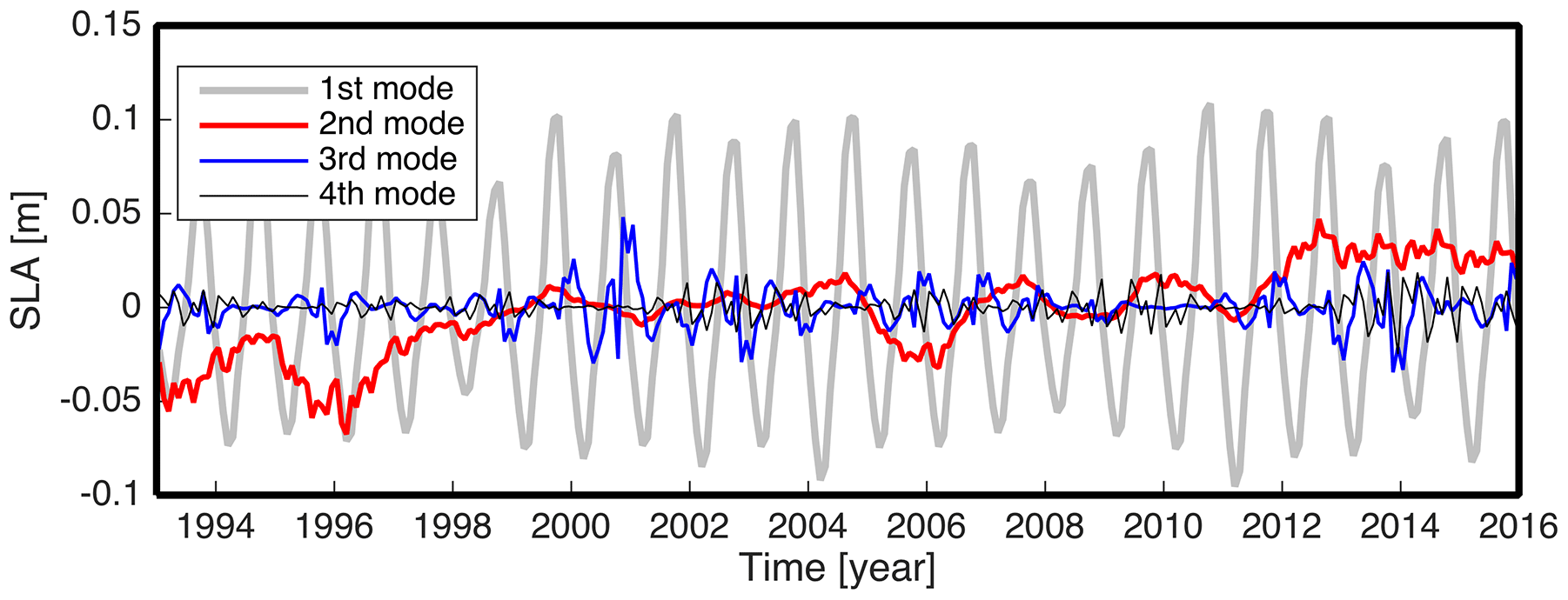
Figure 7Mean SLA of the four biggest modes of CSEOF decomposition of AVISO around the Korean Peninsula.
The linear trend at each TG location was estimated and it was compared with the nearest point in AVISO; using the same data, the ρ values were estimated and the mean value of the ρ was about 0.72 (Fig. 4). In Fig. 4, 11 TG stations (square shapes) have an estimated linear trend at least 30 % less than AVISO, while 21 TG stations (diamond shapes) have an estimated trend exceeding AVISO by more than 30 %. To figure out the effect of these disagreements, the mean SLA of AVISO was compared with the TG's mean SLA, and they showed and NRMSE = 0.52 (Fig. 5). The linear trend of mean SLA of the TGs was estimated as 4.31 mm yr−1 and this value is about 40 % higher than the mean SLA of AVISO (3.1 mm yr−1). This disagreement likely results from the mismatch between locations of TG stations and AVISO grid points, the short time period, and a lack of TGs. Unresolved vertical land motion at the TGs could also lead to such disagreements.
CSEOF decomposition was conducted to investigate the variability of SLA-KP with the 12-month nested period after removing mean values at each grid point. The first mode represents an annual variation considering the spatial patterns and PCT of the CSEOF (Fig. 6a). Nearly 60 % of SLA-KP variations can be presented by the first mode. The second mode shows similar spatial patterns having positive value for all months, and the PCT shows a clear positive trend (Fig. 6b). This mode can be interpreted as representing the rising sea levels, explaining 10 % of variations of SLA-KP roughly. The third and fourth modes were not obviously related to specific modes of variability, explaining only 5 and 3 %, respectively. Using the four modes, we can explain about 70 % of SLA-KP. The first and second modes have a linear trend, but the linear trend in the first mode is negligibly small compared with the signal itself (Fig. 7). Hence, we can say that the second mode is the most important to estimating SLA-KP.
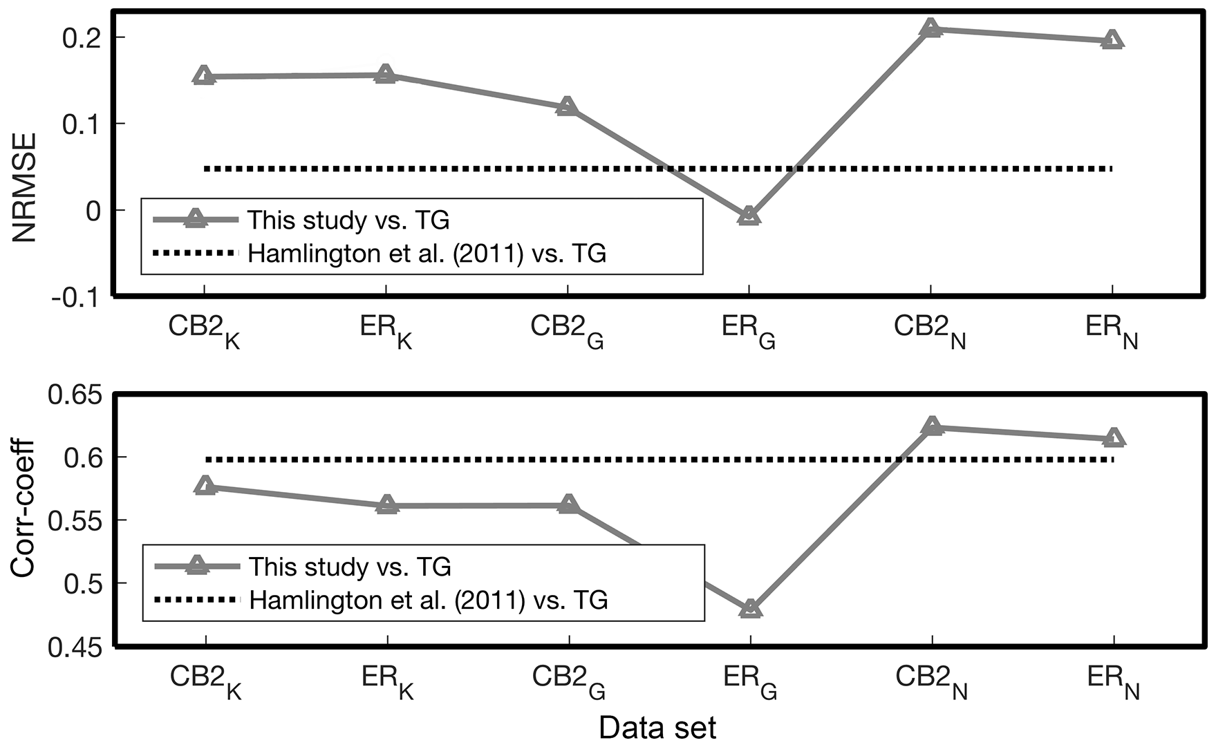
Figure 8Results of the goodness-of-fit test for reconstructed mean SLA according to Hamlington et al. (2011) and TG mean SLA; the top panel includes normalized root mean squared error and the bottom includes the correlation coefficients; here, subscripts K, G, and N represent around the Korean Peninsula, global, and the northwest Pacific, respectively, and CB2 and ER represent COBESST2 and ERSST.
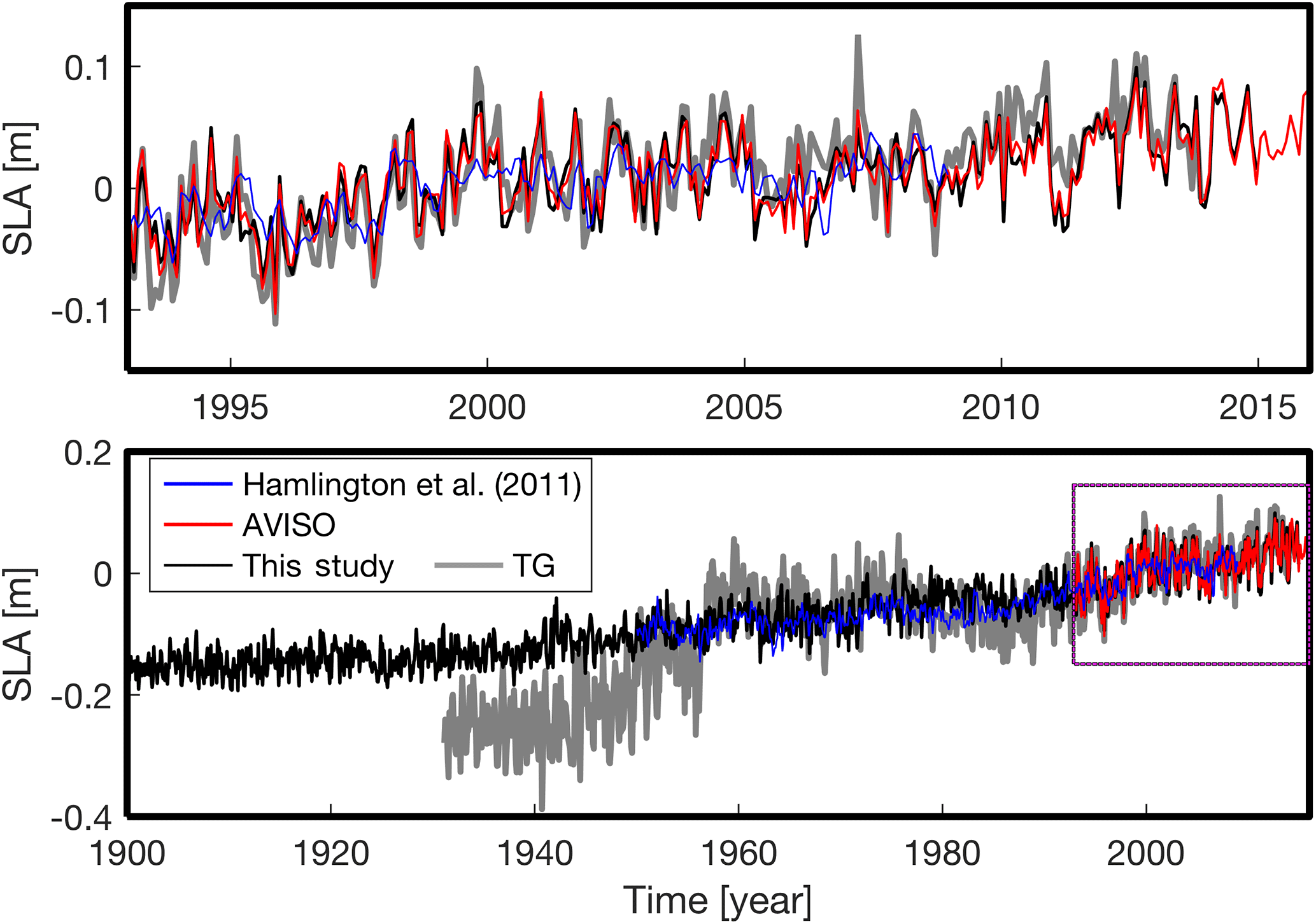
Figure 9Comparison of spatial mean time series of sea level anomalies around the Korean Peninsula without annual signal; the top panel shows the expansion of a box in the bottom panel.
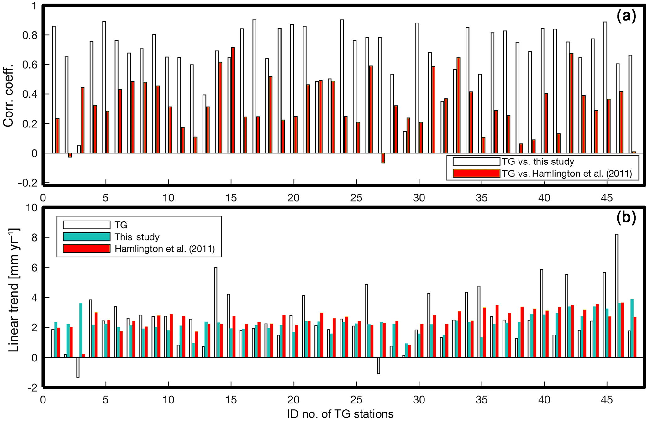
Figure 10(a) Comparison of correlation coefficients between TGs and the reconstructions over 1970–2008; (b) comparison of linear trends over 1970–2008.
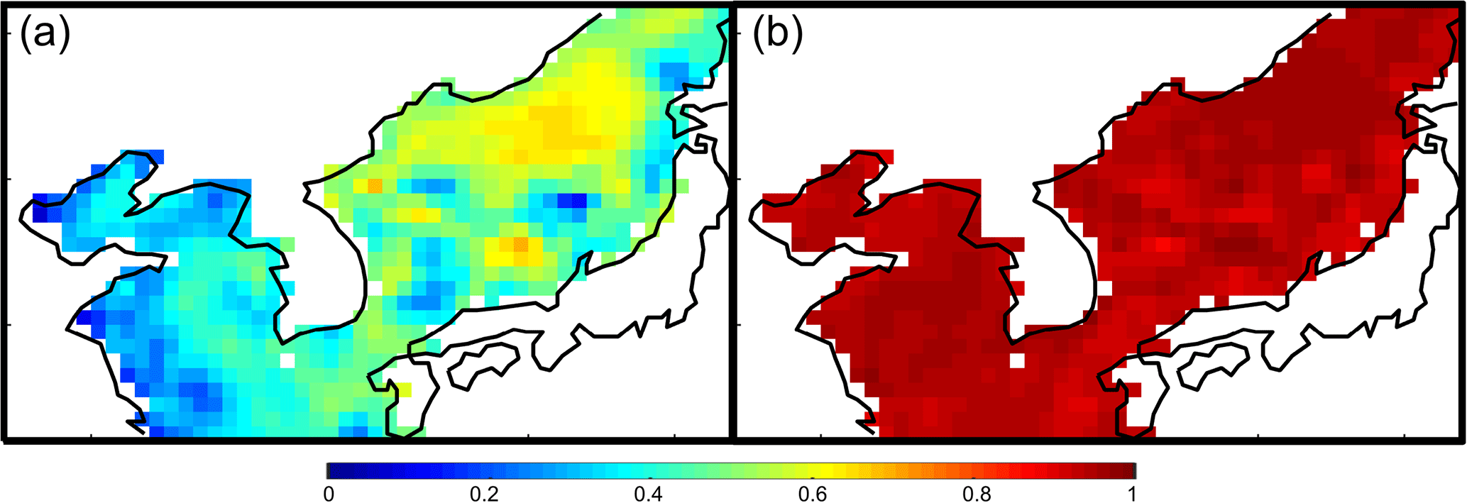
Figure 11(a) Correlation coefficient map between Hamlington et al. (2011) and AVISO over 1993–2008; (b) correlation coefficient map between this study and AVISO over 1993–2008.
3.2 Reconstruction of sea level anomalies
One of the unique characteristics of the current study is that we only used SST as a proxy of former SLA; other studies, however, used TG data or combined data (TG and SST). There are multiple reasons why we chose not to use TG data for the current reconstruction. The first reason is due to both the poor data coverage and the poor data quality. There are relatively few tide gauges extending into the past in our study area and even fewer that are of high quality (i.e., unaffected by vertical land motion, with few gaps, free of non-physical jumps). The second reason, and related to the first, is that due to a methodological characteristic of the CSEOF analysis, a dataset that is free of gaps (temporally continuous) is needed. To satisfy this requirement, we are led to other gridded reconstruction or reanalysis products. There are many types of data that could potentially be used in our scheme (e.g., wind, ocean current, precipitation, atmospheric pressure). We used only SST for the following reasons. (1) SST and SLA have a distinct relationship when we analyze both of them through CSEOF (Hamlington et al., 2011, 2012b, 2016), and Hamlington et al. (2012a) showed that SST could be a good proxy of SLA in this part of the ocean. (2) Limiting our analysis to SST reduces the possibility of overfitting in the regression scheme we use to reconstruct. As a final benefit of using SST, we can check against the available tide gauge data to provide an independent comparison with our reconstruction.
We made six reconstructions (Sect. 2.1.2 and Fig. 8) and compared the six reconstructions with TG over 1970–2008; we could not use complete TG coverage for the comparison because there were only a few TG data available before 1970. Both a correlation coefficient and an NRMSE were applied for the quantified comparison (Fig. 8). Considering the NRMSE, all reconstructions except the global ERSST case provided a better agreement than Hamlington et al. (2011); the best reconstruction was the case of COBESST2 of the northwest Pacific. Regarding correlation coefficient, two reconstructions (COBESST2 of the northwest Pacific and ERSST of the northwest Pacific) showed better results than Hamlington et al. (2011); the reconstruction from COBESST2 of the northwest Pacific provided the best result. Consequently, we selected the reconstruction from COBESST2 of the northwest Pacific as the best reconstruction regarding both NRMSE and correlation coefficient. The mean SLA of the best case showed a reasonable agreement with the mean SLA of TG over 1965–2014 (Fig. 9). For the period before 1965, however, the result showed considerable disagreement.
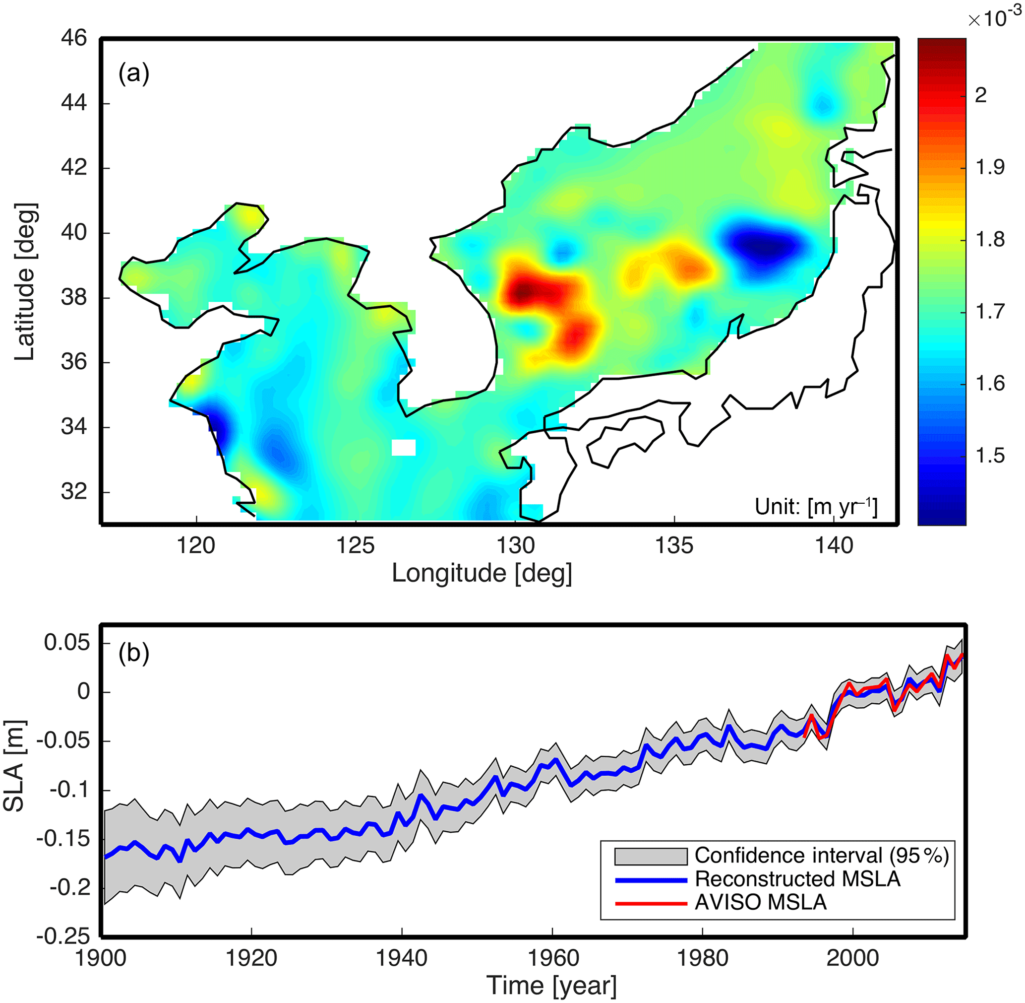
Figure 12(a) Linear trend map of the best reconstruction of the current study from 1900 to 2014; (b) spatial mean time series of sea level anomalies (MSLAs) of the best reconstruction case (COBESST2 of the northwest Pacific) and 95 % confidence interval.
Most of the reconstructions show a better agreement than Hamlington et al. (2011) when considering the correlations with the TGs despite not using TG data during the reconstruction process. The mean of reconstructed SLA shows good agreement with the Hamlington et al. (2011) but poor agreement with the TG (Fig. 9). This disagreement with TG, however, is likely caused by lack of high-quality TGs before 1970. We further calculated correlation coefficients and linear trends using TGs and reconstructions (current study and Hamlington et al., 2011) at each TG location. For the reconstructed data, we calculated the linear trends at the nearest grid points. We made two correlation comparisons: one between this study and TG, and the other between Hamlington et al. (2011) and TG. This study's reconstruction showed higher correlation coefficients than Hamlington et al. (2011), demonstrating the better agreement between the current reconstruction and TG (Fig. 10a). The linear trends of TG, the current reconstruction, and Hamlington et al. (2011) were estimated at the TG locations over 1970 to the present. For the calculation, each time series was edited to have the same time span. The estimated linear trends are given in Fig. 10b. The current study has similar linear trends to Hamlington et al. (2011) at the TG locations, and the variance of the trends are smaller than TG (Fig. 10b). We conducted a t test to check statistical significance of the trend values, and most of values are statistically significant except some values (TG: nos. 2, 3, 29, and 47; Hamlington et al. (2011): no. 3; current study: no. 35). The current study shows a better agreement with AVISO than Hamlington et al. (2011) over the satellite era (Fig. 11). It also has more fluctuations (Fig. 9), and these detailed fluctuations are closer to AVISO, and this is likely a result of two reasons: (1) using a greater number of target modes for the reconstruction process than previous studies (Hamlington et al., 2011, 2012a, b), and (2) considering lagged relations between PCTs. Hamlington et al. (2011, 2012a, b) used a limited number (< 90 % of total variance) of CSEOF modes to avoid overfitting issues, but in this study, we used 19 CSEOF modes which explain 98 % of total variance of SLA-KP by using selective predictors. Further considering lagged relation between targets and predictors, we have a better representation of targets even using fewer predictors.
Using the Monte Carlo simulation, the means and standard deviations of reconstructed SLAs were estimated for the best reconstruction case (COBESST2 of the northwest Pacific). By applying the means and standard deviations of regression coefficients (Eq. 7), each mode's PCT was randomly extended into the past, and the process was repeated a thousand times. The extended PCTs were combined with corresponding LVs of AVISO. Through this process, a thousand SLAs were generated, and the mean and standard deviation were estimated at each time step and grid point. The resulting mean SLA and 95 % confidence interval are shown in Fig. 12. The wider confidence interval of early years is likely due to two reasons: the large uncertainties of observation of SST and the large uncertainties of added GMSL in early years.
The linear trend in the reconstructed SLA over 1900–2014 is estimated as 1.71 ± 0.04 mm yr−1, and this value is similar to the linear trend of Church and White (2011) as 1.70 ± 0.02 mm yr−1. A linear trend map of the reconstructed SLA was calculated, and the maximum and minimum linear trends are about 2.1 and 1.4 mm yr−1, respectively (Fig. 12). The difference, about 0.7 mm yr−1, between two extreme values of the reconstructed SLA is much less than AVISO over 1993–2015 (about 7 mm yr−1), particularly in the Yellow Sea (Figs. 2 and 12). This alleviation means that the extended reconstruction period can reduce the impact of internal variability on estimated trends.
There were two primary goals of the work presented in this study: (1) improve the understanding of the sea level around the KP both in the past and present, and (2) present a new reconstruction scheme for local areas with insufficient tide gauge coverage. To meet these goals, we used the satellite altimeter data over 1993–2015 and the TG data to investigate the characteristics of SLA-KP. The linear trend of SLA-KP was estimated as 3.1 ± 0.5 mm yr−1 from the satellite altimeter data (Fig. 2). However, when we looked into the trend map, some areas (such as near the river mouth in the Yellow Sea and in the middle of the East Sea/Sea of Japan) showed significant departures from the mean trend (Fig. 2).
To investigate this further, the reconstruction was performed using AVISO and two SST reanalysis datasets. Each SST dataset was divided into three cases (global, the northwest Pacific, and KP). The six datasets were decomposed by CSEOF analysis; AVISO was decomposed into CSEOF modes after removing the GMSL. The decomposed LVs played the role of basis functions for the reconstruction, and the main process of reconstruction was extending the PCTs of each mode into the past. Six reconstructions were generated by this study over 1900–2014. Using a correlation coefficient and an NRMSE, the best reconstruction was selected. The best reconstruction was produced by COBESST2 of the northwest Pacific. Through the best reconstruction results, the linear trend of SLA was estimated as 1.71 ± 0.04 mm yr−1 over 1900–2014 (Fig. 12). The extreme linear trends shown in Fig. 2 did not appear in the reconstructed SLA-KP (Figs. 2 and 12).
While we focus here on a specific example (the KP), this study can be used to inform other efforts in studying past and present sea level in areas with poor tide gauge coverage. Our interest was on the KP, specifically, but it was found that including information from the northwest Pacific improved the localized representation of sea level. Consequently, considering large-scale ocean variability and teleconnections between different parts of the ocean is important when selecting the reconstruction domain. This study also demonstrates that TG data may not even be necessary to understand sea level in the past. Using only satellite-based sea level information and SST, we found dramatic improvements between the current reconstruction and past efforts, particularly when comparing to the TG variability. Many TGs are influenced by vertical land motion that cannot easily be corrected for. Relying on SST alleviates concerns associated with non-ocean-related trends. It should be noted that this reconstruction may not work as well in other parts of the ocean, especially those with a less pronounced agreement between sea level and SST. This study does, however, demonstrate the extended efforts that must be made to obtain accurate information about past sea level. As planning efforts get underway in more parts of the world, such comparisons between past and present sea level will become more important, and alternative approaches to simply using TG information are going to be needed.
The reconstructed SLA data is available upon request from Se-Hyeon Cheon (shcheon95@gmail.com).
The authors declare that they have no conflict of interest.
Se-Hyeon Cheon and Kyung-Duck Suh were supported by Basic Science Research Program through
the National Research Foundation of Korea (NRF) funded by the Ministry of
Science, ICT and Future Planning (NRF-2014R1A2A2A01007921). Benjamin D. Hamlington
acknowledges support from NASA PO NNX15AG45G and NNX16AH56G.
Edited by: John M. Huthnance
Reviewed by: Xiangbo Feng and one anonymous referee
AVISO: Mean Sea Level: Aviso+, https://www.aviso.altimetry.fr/en/data/products/ocean-indicators-products/mean-sea-level.html, last access: 1 March 2017. a
Bojariu, R. and Gimeno, L.: The role of snow cover fluctuations in multiannual NAO persistence, Geophys. Res. Lett., 30, 1156, https://doi.org/10.1029/2002GL015651, 2003. a
Calafat, F. M. and Gomis, D.: Reconstruction of Mediterranean sea level fields for the period 1945–2000, Glob. Planet. Change, 66, 225–234, 2009. a
Chambers, D. P., Mehlhaff, C. A., Urban, T. J., Fujii, D., and Nerem, R. S.: Low-frequency variations in global mean sea level: 1950–2000, J. Geophys. Res.-Ocean., 107, 3026, https://doi.org/10.1029/2001JC001089, 2002. a, b
Cheon, S.-H. and Suh, K.-D.: Effect of sea level rise on nearshore significant waves and coastal structures, Ocean Eng., 114, 280–289, 2016. a
Choi, H. and Jeong, M.: Demographic Change in the Coastal Zones, Proceeding of Korean Society for Marine Environment and Energy, p. 115, 2015. a
Church, J. A. and White, N. J.: A 20th century acceleration in global sea-level rise, Geophys. Res. Lett., 33, L01602, https://doi.org/10.1029/2005GL024826, 2006. a, b, c, d, e
Church, J. A. and White, N. J.: Sea-level rise from the late 19th to the early 21st century, Surv. Geophys., 32, 585–602, 2011. a, b, c, d, e, f, g, h
Church, J. A., White, N. J., Coleman, R., Lambeck, K., and Mitrovica, J. X.: Estimates of the regional distribution of sea level rise over the 1950–2000 period, J. Clim., 17, 2609–2625, 2004. a, b
Compo, G. P., Whitaker, J. S., and Sardeshmukh, P. D.: Feasibility of a 100-year reanalysis using only surface pressure data, B. Am. Meteorol. Soc., 87, 175–190, 2006. a
Compo, G. P., Whitaker, J. S., Sardeshmukh, P. D., Matsui, N., Allan, R. J., Yin, X., Gleason, B. E., Vose, R. S., Rutledge, G., Bessemoulin, P., Brönnimann, S., Brunet, M., Crouthamel, R. I., Grant, A. N., Groisman, P. Y., Jones, P. D., Kruk, M. C., Kruger, A. C., Marshall, G. J., Maugeri, M., Mok, H. Y., Nordli, Ø., Ross, T. F., Trigo, R. M., Wang, X. L., Woodruff, S. D., and Worley, S. J.: The twentieth century reanalysis project, Q. J. Roy. Meteor. Soc., 137, 1–28, 2011. a
Dettinger, M. D., Cayan, D. R., Diaz, H. F., and Meko, D. M.: North–south precipitation patterns in western North America on interannual-to-decadal timescales, J. Clim., 11, 3095–3111, 1998. a
Dommenget, D. and Latif, M.: A cautionary note on the interpretation of EOFs, J. Clim., 15, 216–225, 2002. a
Hamlet, A. F., Mote, P. W., Clark, M. P., and Lettenmaier, D. P.: Effects of temperature and precipitation variability on snowpack trends in the western United States, J. Clim., 18, 4545–4561, 2005. a
Hamlington, B., Leben, R., Nerem, R., Han, W., and Kim, K.-Y.: Reconstructing sea level using cyclostationary empirical orthogonal functions, J. Geophys. Res.-Ocean., 116, C12015, https://doi.org/10.1029/2011JC007529, 2011. a, b, c, d, e, f, g, h, i, j, k, l, m, n, o, p, q, r, s, t, u, v, w, x, y
Hamlington, B., Leben, R., and Kim, K.-Y.: Improving sea level reconstructions using non-sea level measurements, J. Geophys. Res.-Ocean., 117, C10025, https://doi.org/10.1029/2012JC008277, 2012a. a, b, c, d, e, f, g
Hamlington, B., Leben, R., Wright, L., and Kim, K.-Y.: Regional sea level reconstruction in the Pacific ocean, Mar. Geod., 35, 98–117, 2012b. a, b, c, d, e, f
Hamlington, B., Cheon, S., Thompson, P., Merrifield, M., Nerem, R., Leben, R., and Kim, K.-Y.: An ongoing shift in Pacific Ocean sea level, J. Geophys. Res.-Ocean., 121, 5084–5097, 2016. a
Hendon, H. H., Wheeler, M. C., and Zhang, C.: Seasonal dependence of the MJO–ENSO relationship, J. Clim., 20, 531–543, 2007. a
Hirahara, S., Ishii, M., and Fukuda, Y.: Centennial-scale sea surface temperature analysis and its uncertainty, J. Clim., 27, 57–75, 2014. a
Huang, B., Banzon, V. F., Freeman, E., Lawrimore, J., Liu, W., Peterson, T. C., Smith, T. M., Thorne, P. W., Woodruff, S. D., and Zhang, H.-M.: Extended reconstructed sea surface temperature version 4 (ERSST, v4), Part I: Upgrades and intercomparisons, J. Clim., 28, 911–930, 2015. a
Huang, B., Thorne, P. W., Smith, T. M., Liu, W., Lawrimore, J., Banzon, V. F., Zhang, H.-M., Peterson, T. C., and Menne, M.: Further exploring and quantifying uncertainties for extended reconstructed sea surface temperature (ERSST) version 4 (v4), J. Clim., 29, 3119–3142, 2016. a
Ishii, M., Shouji, A., Sugimoto, S., and Matsumoto, T.: Objective analyses of sea-surface temperature and marine meteorological variables for the 20th century using ICOADS and the Kobe collection, Int. J. Climatol., 25, 865–879, 2005. a
Kaplan, A., Cane, M. A., Kushnir, Y., Clement, A. C., Blumenthal, M. B., and Rajagopalan, B.: Analyses of global sea surface temperature 1856–1991, J. Geophys. Res.-Ocean., 103, 18567–18589, 1998. a
Kaplan, A., Kushnir, Y., and Cane, M. A.: Reduced space optimal interpolation of historical marine sea level pressure: 1854–1992, J. Clim., 13, 2987–3002, 2000. a
Kawamura, R., Suppiah, R., Collier, M. A., and Gordon, H. B.: Lagged relationships between ENSO and the Asian Summer Monsoon in the CSIRO coupled model, Geophys. Res. Lett., 31, L23205, https://doi.org/10.1029/2004GL021411, 2004. a
Kim, K.-Y. and Chung, C.: On the evolution of the annual cycle in the tropical Pacific, J. Clim., 14, 991–994, 2001. a
Kim, K.-Y. and North, G. R.: EOFs of harmonizable cyclostationary processes, J. Atmos. Sci., 54, 2416–2427, 1997. a, b, c
Kim, K.-Y. and Wu, Q.: A comparison study of EOF techniques: Analysis of nonstationary data with periodic statistics, J. Clim., 12, 185–199, 1999. a, b
Kim, K.-Y., North, G. R., and Huang, J.: EOFs of one-dimensional cyclostationary time series: Computations, examples, and stochastic modeling, J. Atmos. Sci., 53, 1007–1017, 1996. a, b, c
Kim, K.-Y., Hamlington, B., and Na, H.: Theoretical foundation of cyclostationary EOF analysis for geophysical and climatic variables: concepts and examples, Earth-Sci. Rev., 150, 201–218, 2015. a, b, c, d
Liu, W., Huang, B., Thorne, P. W., Banzon, V. F., Zhang, H.-M., Freeman, E., Lawrimore, J., Peterson, T. C., Smith, T. M., and Woodruff, S. D.: Extended reconstructed sea surface temperature version 4 (ERSST. v4): Part II. Parametric and structural uncertainty estimations, J. Clim., 28, 931–951, 2015. a
McPhaden, M. J., Zhang, X., Hendon, H. H., and Wheeler, M. C.: Large scale dynamics and MJO forcing of ENSO variability, Geophys. Res. Lett., 33, L16702, https://doi.org/10.1029/2006GL026786, 2006. a
Nicholls, R. J.: Planning for the impacts of sea level rise, Oceanography, 24, 142–155, https://doi.org/10.5670/oceanog.2011.34, 2011. a, b
Peltier, W.: Global glacial isostasy and the surface of the ice-age Earth: the ICE-5G (VM2) model and GRACE, Annu. Rev. Earth Pl. Sc., 32, 111–149, 2004. a
Redmond, K. T. and Koch, R. W.: Surface climate and streamflow variability in the western United States and their relationship to large-scale circulation indices, Water Resour. Res., 27, 2381–2399, 1991. a
Suh, K.-D., Kim, S.-W., Kim, S., and Cheon, S.: Effects of climate change on stability of caisson breakwaters in different water depths, Ocean Eng., 71, 103–112, 2013. a