the Creative Commons Attribution 4.0 License.
the Creative Commons Attribution 4.0 License.
 | 08 Aug 2018
Frictional interactions between tidal constituents in tide-dominated estuaries
Huayang Cai
Marco Toffolon
Hubert H. G. Savenije
Qingshu Yang
When different tidal constituents propagate along an estuary, they interact because of the presence of nonlinear terms in the hydrodynamic equations. In particular, due to the quadratic velocity in the friction term, the effective friction experienced by both the predominant and the minor tidal constituents is enhanced. We explore the underlying mechanism with a simple conceptual model by utilizing Chebyshev polynomials, enabling the effect of the velocities of the tidal constituents to be summed in the friction term and, hence, the linearized hydrodynamic equations to be solved analytically in a closed form. An analytical model is adopted for each single tidal constituent with a correction factor to adjust the linearized friction term, accounting for the mutual interactions between the different tidal constituents by means of an iterative procedure. The proposed method is applied to the Guadiana (southern Portugal–Spain border) and Guadalquivir (Spain) estuaries for different tidal constituents (M2, S2, N2, O1, K1) imposed independently at the estuary mouth. The analytical results appear to agree very well with the observed tidal amplitudes and phases of the different tidal constituents. The proposed method could be applicable to other alluvial estuaries with a small tidal amplitude-to-depth ratio and negligible river discharge.
- Article
(7511 KB) - Full-text XML
-
Supplement
(56 KB) - BibTeX
- EndNote


Numerous studies have been conducted in recent decades to model tidal wave propagation along an estuary since an understanding of tidal dynamics is essential for exploring the influence of human-induced (such as dredging for navigational channels) or natural (such as global sea level rises) interventions on estuarine environments (Schuttelaars et al., 2013; Winterwerp et al., 2013). Analytical models are invaluable tools and have been developed to study the basic physics of tidal dynamics in estuaries; for instance, to examine the sensitivity of tidal properties (e.g., tidal damping or wave speed) to change in terms of external forcing (e.g., spring–neap variations in amplitude) and geometry (e.g., depth or channel length). However, most analytical solutions developed to date, which make use of the linearized Saint-Venant equations, can only deal with one predominant tidal constituent (e.g., M2), which prevents consideration of the nonlinear interactions between different tidal constituents. The underlying problem is that the friction term in the momentum equation follows a quadratic friction law, which causes nonlinear behavior, causing tidal asymmetry as the tide propagates upstream. If the friction law were linear, one would expect that the effective frictional effect for different tidal constituents (e.g., M2 and S2) could be computed independently (Pingree, 1983).
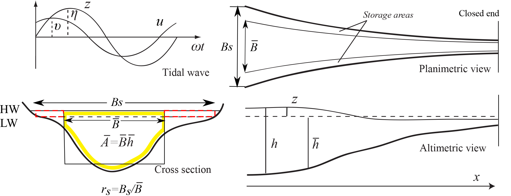
Figure 1Geometry of a semi-closed estuary and basic notation (after Savenije et al., 2008). HW, high water; LW, low water.
To explore the interaction between different constituents of the tidal flow, the quadratic velocity (where u is the velocity) is usually approximated by a truncated series expansion, such as a Fourier expansion (Proudman, 1953; Dronkers, 1964; Le Provost, 1973; Pingree, 1983; Fang, 1987; Inoue and Garrett, 2007). If the tidal current is composed of one dominant constituent and a much smaller second constituent, it has been shown by many researchers (Jeffreys, 1970; Heaps, 1978; Prandle, 1997) that the weaker constituent is acted on by up to 50 % more friction than acts on the dominant constituent. However, this requires the assumption of a very small value of the ratio of the magnitudes of the weaker and dominant constituents, which indicates that this is only a first-order estimation. Later, some researchers extended the analysis to improve the accuracy of estimates and to allow for more than two constituents (Pingree, 1983; Fang, 1987; Inoue and Garrett, 2007). Pingree (1983) investigated the interaction between M2 and S2 tides, resulting in a second-order correction of the effective friction coefficient acting on the predominant M2 tide and a fourth-order value for the weaker S2 constituent of the tide. Fang (1987) derived exact expressions of the coefficients of the Fourier expansion of for two tidal constituents but did not provide exact solutions for the case of three or more constituents. Later, Inoue and Garrett (2007) used a novel approach to determine the Fourier coefficients of , which allows the magnitude of the effective friction coefficient to be determined for many tidal constituents. For the general two-dimensional tidal wave propagation, the expansion of quadratic bottom friction using a Fourier series was first proposed by Le Provost (1973) and subsequently applied to spectral models for regional tidal currents (Le Provost et al., 1981; Le Provost and Fornerino, 1985; Molines et al., 1989). Building on the previous work by Le Provost (1973), the importance of quadratic bottom friction in tidal propagation and damping was discussed by Kabbaj and Le Provost (1980) and reviews of friction terms in models were presented by Le Provost (1991).
In contrast, as noted by other researchers (Doodson, 1924; Dronkers, 1964; Godin, 1991, 1999), the quadratic velocity is, mathematically, an odd function, and it is possible to approximate it by using a two- or three-term expression, such as αu+βu3 or , where α, β and ξ are suitable numerical constants. The linear term αu represents the linear superposition of different constituents, while the nonlinear interaction is attributed to a cubic term βu3 and a fifth-order term ξu5. It is to be noted that such a method has the advantage of keeping the hydrodynamic equations solvable in a closed form (Godin, 1991, 1999).
Previous studies explored the effect of frictional interaction between different tidal constituents by quantifying a friction correction factor only (e.g., Dronkers, 1964; Le Provost, 1973; Pingree, 1983; Fang, 1987; Godin, 1999; Inoue and Garrett, 2007). In this study, for the first time, the mutual interactions between tidal constituents in the frictional term were explored using a conceptual analytical model. Specifically, a friction correction factor for each constituent was defined by expanding the quadratic velocity using a Chebyshev polynomials approach. The model has subsequently been applied to the Guadiana and Guadalquivir estuaries in southern Iberia, for which cases the mutual interaction between the predominant M2 tidal constituent and other tidal constituents (e.g., S2, N2, O1, K1) is explored.
2.1 Hydrodynamic model
We are considering a semi-closed estuary that is forced by one predominant tidal constituent (e.g., M2) with the tidal frequency , where T is the tidal period. As the tidal wave propagates into the estuary, it has a wave celerity of water level cA, a wave celerity of velocity cV, an amplitude of tidal elevation η, a tidal velocity amplitude υ, a phase of water level ϕA, and a phase of velocity ϕV. The length of the estuary is indicated by Le.
The geometry of a semi-closed estuary is shown in Fig. 1, where x is the longitudinal coordinate, which is positive in the landward direction, and z is the free surface elevation. The tidally averaged cross-sectional area and width are assumed to be exponentially convergent in the landward direction, as described by
where and are the respective values at the estuary mouth (where x=0) and a and b are the convergence lengths of cross-sectional area and width, respectively. We also assume a rectangular cross section, from which it follows that the tidally averaged depth is given by . The possible influence of storage area is described by the storage width ratio rS, defined as the ratio of the storage width BS (width of the channel at averaged high water level) to the tidally averaged width (i.e., ).
With the above assumptions, the one-dimensional continuity equation reads
where t is the time and h the instantaneous depth. Assuming negligible density effects, the one-dimensional momentum equations can be cast as follows
where g is the acceleration due to gravity and K is the Manning–Strickler friction coefficient.
In order to obtain an analytical solution, we assume a negligible river discharge and that the tidal amplitude is small with respect to the mean depth and follow Toffolon and Savenije (2011) to derive the linearized solution of the system of Eqs. (1) and (2). However, different from the standard linear solutions, we will retain the mutual interaction among different harmonics originating from the nonlinear frictional term, which contains two sources of nonlinearity: the quadratic velocity and the variable depth in the denominator. While we neglect the latter factor, consistent with the assumption of small tidal amplitude, we will exploit Chebyshev polynomials to represent the harmonic interaction in the quadratic velocity (see Sect. 3.1). For clarity, we report here the linearized version of the momentum equation
and the friction coefficient
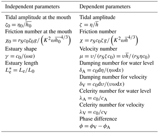
Toffolon and Savenije (2011) demonstrated that the tidal hydrodynamics in a semi-closed estuary are controlled by a few dimensionless parameters that depend on geometry and external forcing (for detailed information about analytical solutions for tidal hydrodynamics, readers can refer to Appendix Appendix A). They are defined in Table 1 and can be interpreted as follows: ζ0 is the dimensionless tidal amplitude (the subscript 0 indicating the seaward boundary condition); γ is the estuary shape number (representing the effect of cross-sectional area convergence); χ0 is the friction number (describing the role of the frictional dissipation); is the dimensionless estuary length. The dimensional quantities used in the definition of the dimensionless parameters are as follows: η0 is the tidal amplitude at the seaward boundary; is the frictionless wave celerity in a prismatic channel; is the tidal length scale related to the frictionless tidal wave length by a factor 2π.
The main dependent dimensionless parameters are also presented in Table 1, including the following: ζ is the actual tidal amplitude; χ is the actual friction number; μ is the velocity number (the ratio of the actual velocity amplitude to the frictionless value in a prismatic channel); λA and λV are, respectively, the celerity for elevation and velocity (the ratio between the frictionless wave celerity in a prismatic channel and actual wave celerity); δA and δV are, respectively, the amplification number for elevation and velocity (describing the rate of increase, δA (or δV)>0, or decrease, δA (or δV)<0, in the wave amplitudes along the estuary axis); is the phase difference between the phases of velocity and elevation.
It is important to remark that several nonlinear terms are present both in the continuity and in the momentum equations (Parker, 1991), which are responsible, for instance, for the internal generation of overtides (e.g., M4). In this approximated approach, we disregard them and focus exclusively on the mutual interaction among the external tidal constituents mediated by the quadratic velocity dependence in the frictional term. In fact, the nonlinear quadratic velocity term crucially affects the propagation of the tidal waves associated with the different constituents that are already present in the tidal forcing at the estuary mouth.
2.2 Study areas
Both the Guadiana and Guadalquivir estuaries are located in the southwest part of the Iberian Peninsula. These systems are good candidates for the application of a 1-D hydrodynamic model of tidal propagation. Both estuaries feature a simple geometry, consisting of a single, narrow and moderately deep channel with relatively smooth bathymetric variations. Moreover, their tidal prism exceeds their average freshwater inputs by several orders of magnitude due to strong regulation by dams. Under these usual, low river discharge conditions, both estuaries are well-mixed, and the water circulation is mainly driven by tides.
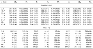
The Guadiana estuary, at the southern border between Spain and Portugal, connects the Guadiana River to the Gulf of Cádiz. Tidal water level oscillations are observed along the channel as far as a weir 78 km upstream of the river mouth (Garel et al., 2009). Both the cross-sectional area and the channel width are convergent and can be described by an exponential function, with convergence lengths of a=31 km and b=38 km, respectively (Fig. 2). The flow depth is generally between 4 and 8 m, with a mean depth of about 5.5 m (Garel, 2017). The tidal dynamics in the Guadiana estuary are derived from records obtained using eight pressure transducers deployed for a period of 2 months (31 July to 25 September 2015) approximately every 10 km along the estuary (from the mouth to ∼70 km upstream). The data were collected during an extended (months-long) period of drought with negligible river discharge (always <20 m3 s−1 over the preceding 5 months). For each station, the amplitude and phase of elevation of the tidal constituents were obtained from standard harmonic analysis of the observed pressure records using the “t-tide” Matlab toolbox (Pawlowicz et al., 2002). The harmonic results are displayed in Table 2. Near the mouth, the largest diurnal (K1), semidiurnal (M2) and quarter-diurnal (M4) frequencies are similar to those previously reported at the same location based on pressure records taken over ∼9 months (see Garel and Ferreira, 2013). In particular, the value is less than 0.1 at the sea boundary, which indicates that the tide is dominantly semidiurnal.
The Guadalquivir estuary is located in southern Spain, at ∼100 km to the east of the Guadiana River mouth. The estuary has a length of 103 km starting from the mouth at Sanlúcar de Barrameda to the Alcalá del Río dam. The geometry of the Guadalquivir estuary can be approximated by exponential functions with a convergence length of a=60 km for the cross-sectional area and b=66 km for the width (see Diez-Minguito et al., 2012). The flow depth is more or less constant (7.1 m).
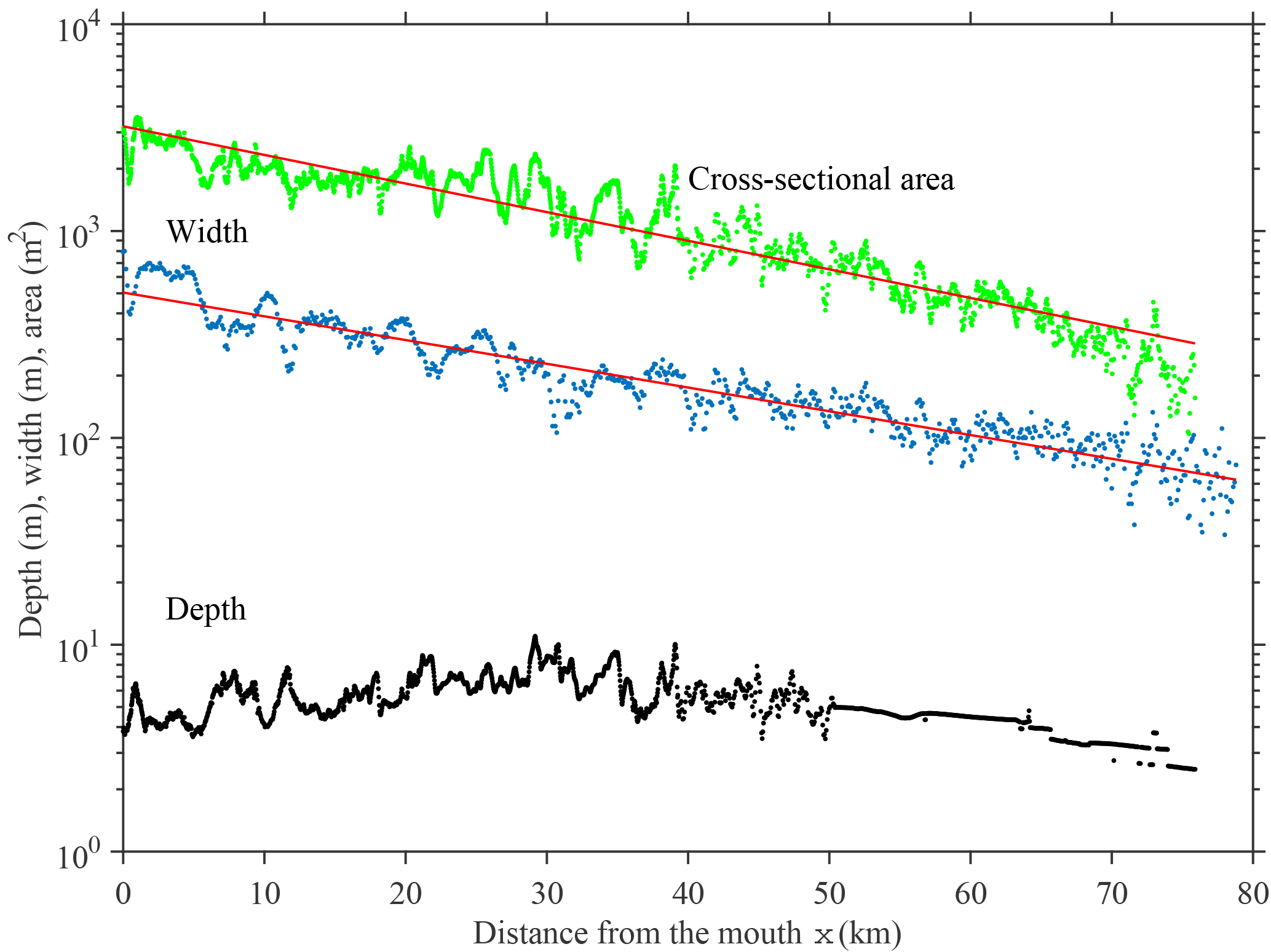
Figure 2Tidally averaged depth (m, black dots), width (m, blue dots) and cross-sectional area (m2, green dots) along the Guadiana estuary. Red lines represent exponential fit curves for the width and cross-sectional area.
Table 2Tidal elevation amplitudes (m) and phases (∘) estimates (with 95 % confidence intervals in brackets) from harmonic analyses of pressure records along the Guadiana estuary (x: distance from the mouth, km).
Tidal dynamics along the Guadalquivir estuary were analyzed by Diez-Minguito et al. (2012) based on harmonic analyses of field measurements collected from June to December 2008. The amplitude and phase of tidal constituents near the mouth are highly similar to those at the entrance of the Guadiana estuary (Table 2), producing a semidiurnal and mesotidal signal with a mean spring tidal range of 3.5 m. In this paper, the tidal observations of the Guadalquivir estuary are taken directly from Diez-Minguito et al. (2012). The results apply to the low river discharge conditions (<40 m3 s−1) that usually predominate in the estuary.
3.1 Representation of quadratic velocity using the Chebyshev polynomials approach
Chebyshev polynomials can be used to approximate the quadratic dependence of the friction term on the velocity, . Adopting a two-term approximation, it is known that (Godin, 1991, 1999)
where is the sum of the amplitudes of all the harmonic constituents. The Chebyshev coefficients and were determined by the expansion of cos (nx) (n=1, 2, …) in powers of cos (x) (Godin, 1991, 1999). It is important to note that, unlike series developments (e.g., Fourier expansion), the Chebyshev coefficients α and β vary with the number of terms that are used in the development. Godin (1991) already showed that a two-term approximation (such as Eq. 5) is adequate to satisfactorily account for the friction.
For a single harmonic
where υ1 is the velocity amplitude and ω1 its frequency, Eq. (5) can be expressed by exploiting standard trigonometric relations as
Focusing only on the original harmonic constituent leads to
which coincides exactly with Lorentz's classical linearization (Lorentz, 1926) or a Fourier expansion of (Proudman, 1953).
Considering a second tidal constituent, the velocity is given by
where υ2 and ω2 are the amplitude and frequency of the second constituent, and and are the ratios of the amplitudes to that of the maximum possible velocity . Note that the possible phase lag between the two constituents is neglected assuming a suitable time shift (Inoue and Garrett, 2007). In this case, the truncated Chebyshev polynomials approximation of (focusing on two original tidal constituents) is expressed as (see also Godin, 1999)
with
where F1 and F2 represent the effective friction coefficients caused by the nonlinear interactions between tidal constituents. The last equality in Eqs. (10) and (10) is due to the fact that . It is worth noting that Eq. (9) is a reasonable approximation only if the amplitude of the secondary constituent is much smaller than that of the dominant one.
For illustration, approximations using Eqs. (5) and (9) for a typical tidal current with and are displayed in Fig. 3 for the case of two tidal constituents. It can be seen that the Chebyshev polynomials approximation (Eq. 5) matches the nonlinear quadratic velocity well, while Eq. (9), retaining only the original frequencies (ω1 and ω2), is still able to approximately capture the first-order trend of the quadratic term.
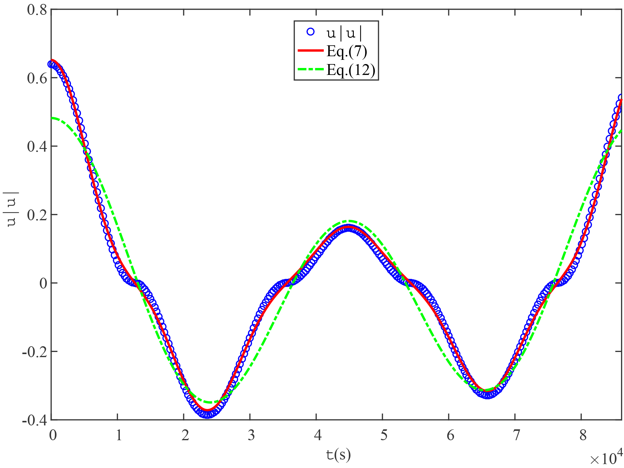
Figure 3Approximation to the quadratic velocity by the Chebyshev polynomials approach for the case of two tidal constituents (i.e., M2 and K1). Here, , where ω1 and ω2 represent the tidal frequencies of M2 and K1, respectively.
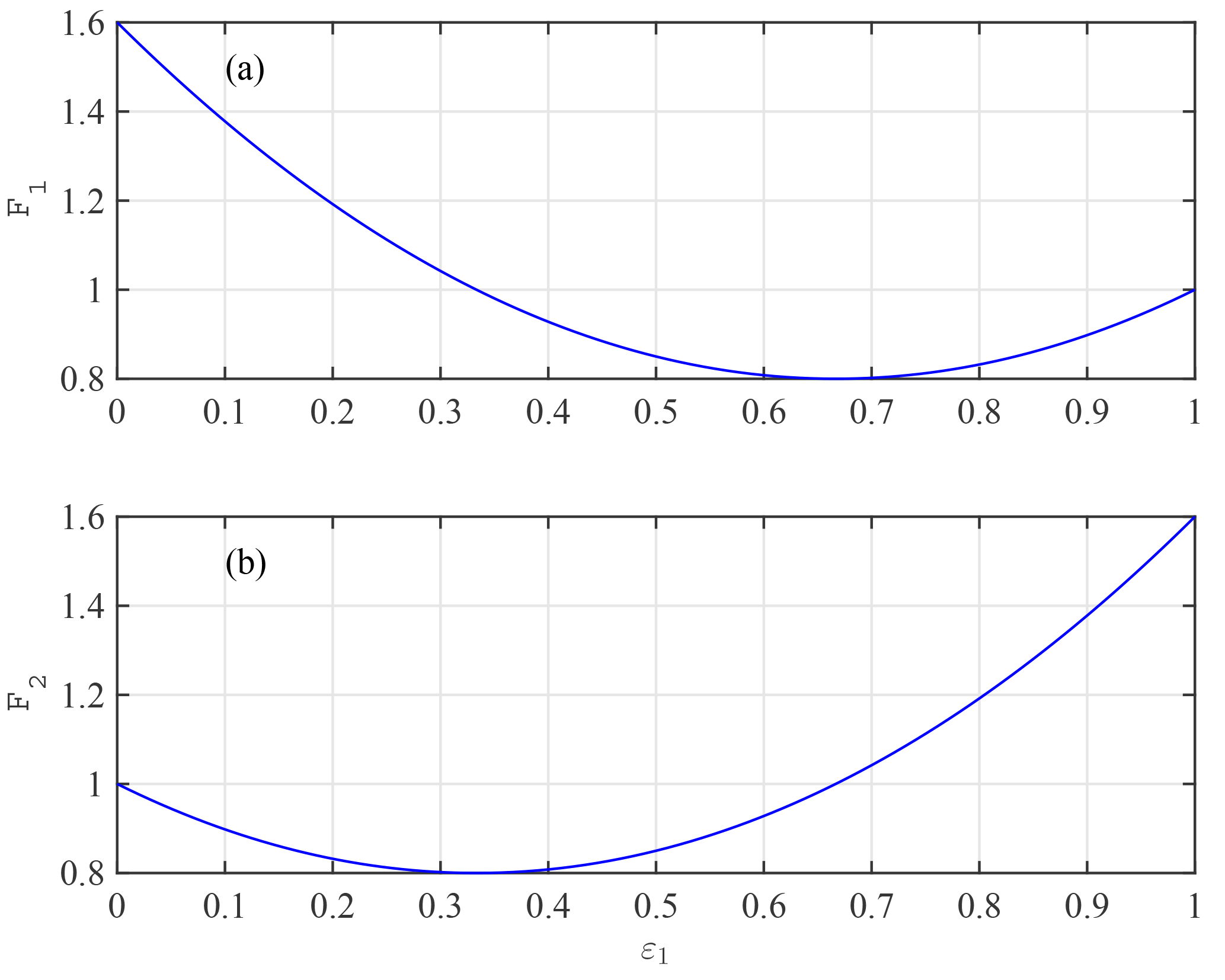
It can be seen from Eqs. (10) and (10) that when ε2≪1 (hence, ε1≃1 for the dominant tidal constituent), F1≃1, F2≃1.6; thus, the weaker constituent experiences proportionately 60 % more friction than the dominant constituent, which is slightly larger than the classical result of 50 % more friction for the weaker tidal constituent. Figure 4 shows the solutions of effective friction coefficients F1 and F2 as a function of ε1 for the case of two constituents. As expected, we see a symmetric response of these coefficients in the function of ε1 since . Specifically, we note that the effective friction coefficient F1 reaches a minimum when , when the velocity amplitude of the dominant constituent is twice as large as the weaker constituent.
Similarly, we are able to extend the same approach to the case of a generic number n of astronomical tidal constituents (e.g., K1, O1, M2, S2, N2):
in which the subscript i represents the ith tidal constituent. Considering only the original tidal constituents, the quadratic velocity can be approximated as
and the general expression for the effective friction coefficients of jth tidal constituents is given by
We provide the complete coefficients for the cases of one to three constituents in Appendix Appendix B.
3.2 Effective friction in the momentum equation
For a single tidal constituent u=υ1cos (ω1t), the quadratic velocity term is often approximated by adopting Lorentz's linearization equation (Eq. 8), and thus the friction term in Eq. (3) becomes
which is the “standard” case for a monochromatic wave, i.e., when we only deal with a predominant tidal constituent (e.g., M2).
For illustration of the method, we consider a tidal current that is composed of one dominant constituent (e.g., M2 with velocity u1) and a weaker constituent (e.g., S2 with velocity u2), which is a simple but important example in estuaries, i.e., . In this case, the combination of Eq. (3) and the Chebyshev polynomials expansion of (Eq. 9) yields
where z1 is the free surface elevation for the dominant constituent and z2 for the secondary constituent. Exploiting the linearity of Eq. (13), we can solve the two problems independently. As a result, we see that the actual friction term that is felt in Eq. (13) is different from that which would be felt by the single constituent alone (Eq. 12).
Introducing a general form of the linearized momentum equation for the generic ith constituent
with
as in the standard case, we see that the effective friction term contains a correction factor
through the coefficient Fi. Since the ratio εi can be quite small for a weaker constituent, the friction actually felt can be significantly stronger.
4.1 Hydrodynamic modeling incorporating the friction correction factor
If there are many tidal constituents, then the friction experienced by one is affected by the others. As suggested by our conceptual model, the mutual effects can be incorporated by using the friction correction factor fn defined in Eq. (16) if the other (weaker) constituents are treated in the same way as the predominant constituent. As a result, the friction number χn for each tidal constituent can be modified as
where χ is the friction number (see definition in Table 1) experienced if only a single tidal constituent is considered.
We note that the modified friction number χn in Eq. (17) contains the friction coefficient K. In many applications, K is calibrated separately for each tidal constituent to account for the different friction exerted due to the combined tide, either changing K directly or through calibration of the different correction friction factors fn (see, e.g., Cai et al., 2015, 2016). The current study aims at avoiding the need to adjust K individually, so that only a single value of K needs to be calibrated, based on the physical consideration that friction mostly depends on bottom roughness, and the other factors (tide interaction) are to be correctly modeled.
4.2 Procedure to study the propagation of the different constituents
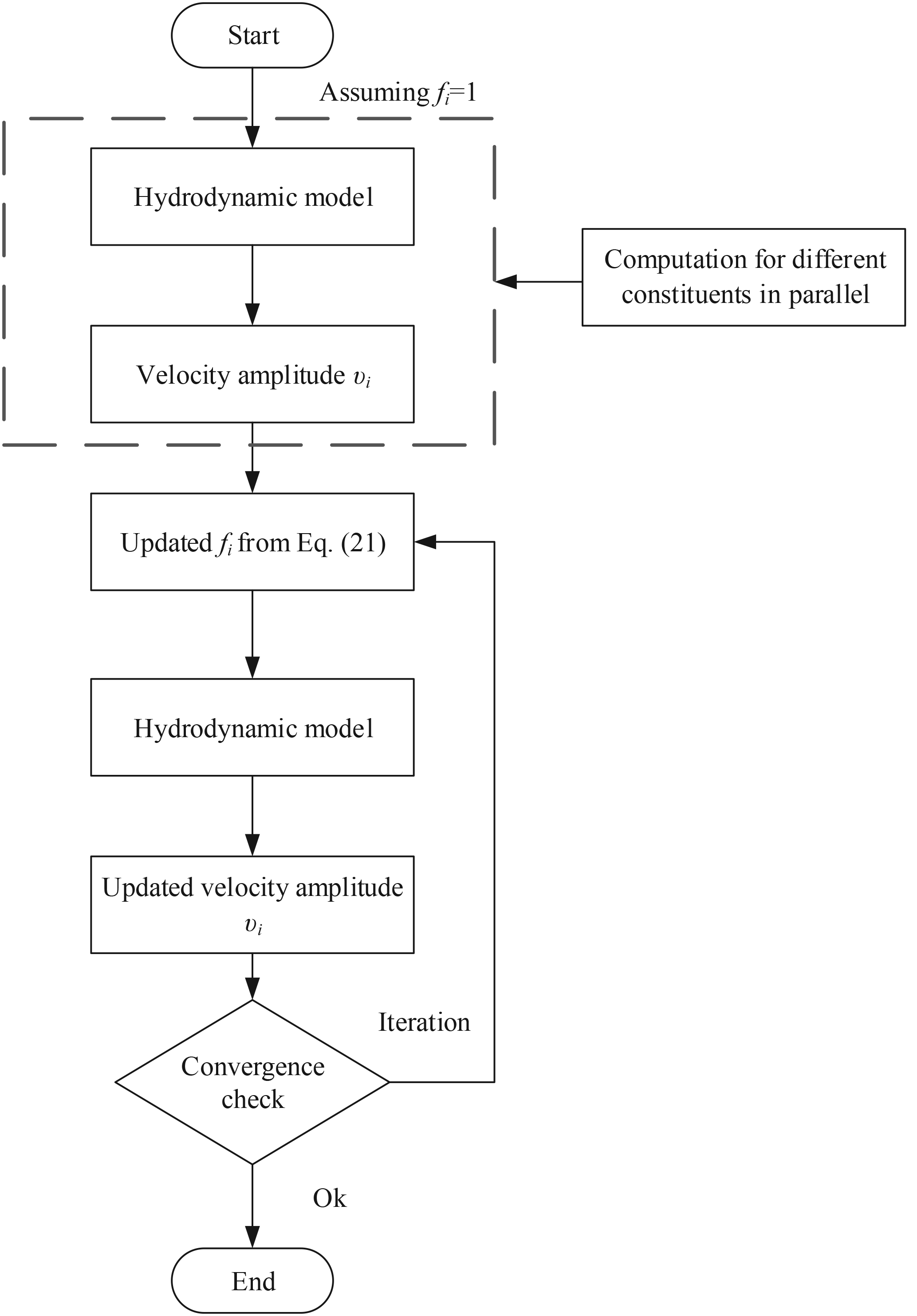
With a hydrodynamic model for a single constituent (see Appendix Appendix A), an iterative procedure can be designed to study the propagation of the different constituents by calibrating a single value of the Manning–Strickler friction parameter K. The flowchart illustrating the computation process is presented in Fig. 5. Initially, we assume the friction correction factor fi=1 for each tidal constituent and compute the first tentative values of velocity amplitude υi along the channel using the hydrodynamic model. This allows defining and, hence, εi. Taking into account the frictional interaction between tidal constituents, the revised fi is calculated using Eqs. (12) and (16). Subsequently, using the updated fi, the new velocity amplitude υi along the channel can be computed using the hydrodynamic model. This process is repeated until the result is stable. In this paper, two examples of Matlab scripts are provided together with the observed tidal data in the Guadiana and Guadalquivir estuaries (see Supplement).
It is worth stressing that the single constituents are not calibrated independently, as was done in previous analyses (e.g., Cai et al., 2015). Conversely, only a single friction parameter, K, is calibrated or estimated based on the physical knowledge of the system (bed roughness). This feature represents a major advantage of the proposed method because the frictional interaction is modeled in mechanistic terms using Eq. (16).
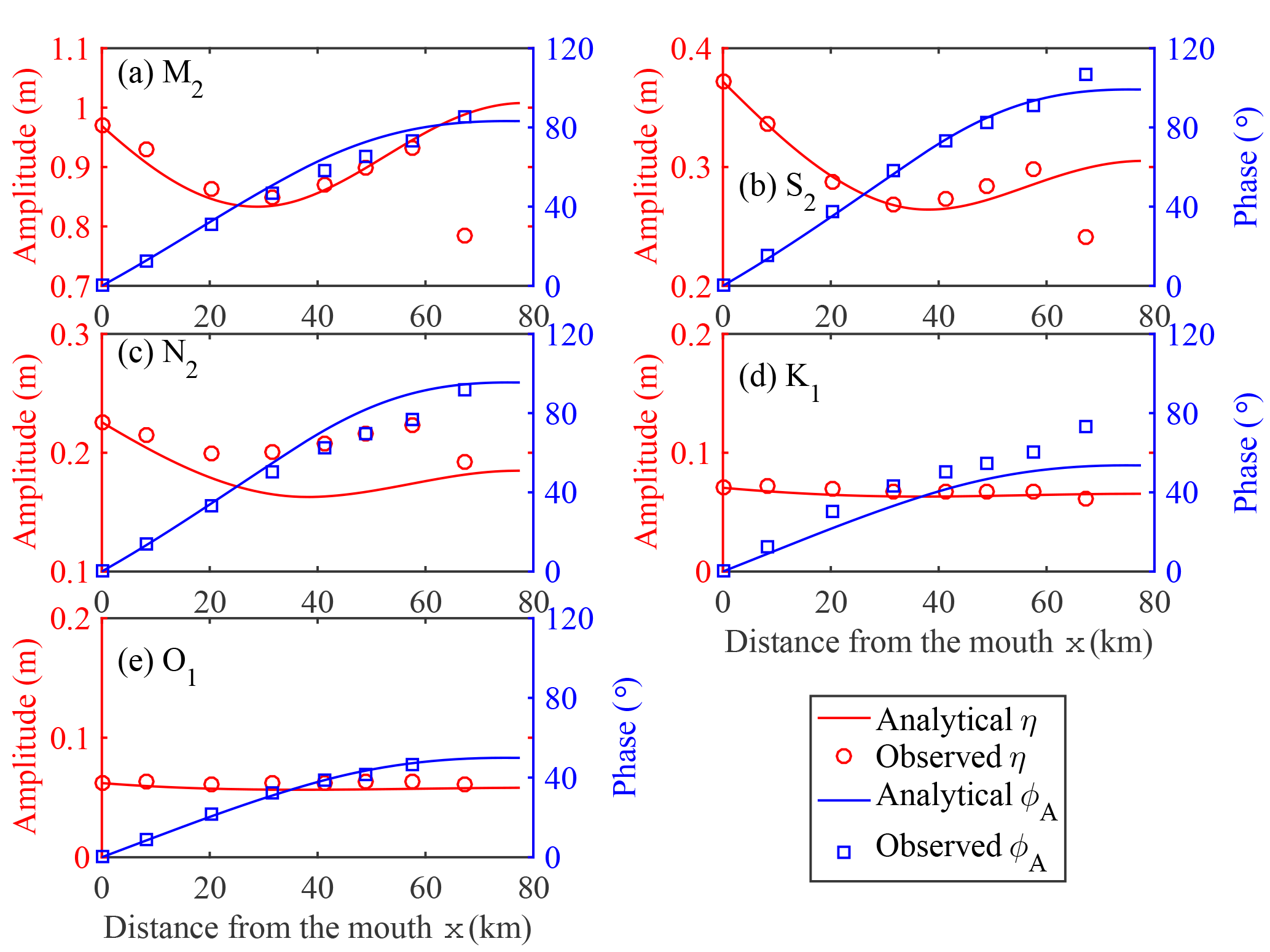
Figure 6Tidal constituents (a) M2, (b) S2, (c) N2, (d) K1 and (e) O1, modeled against observed values of tidal amplitude (m) and phase (∘) of elevation along the Guadiana estuary.
4.3 Application to the Guadiana and Guadalquivir estuaries
In this study, the analytical model for a semi-closed estuary presented in Sect. 2.1 was applied to the Guadiana and Guadalquivir estuaries to reproduce the correct tidal behavior for different tidal constituents. The analytical results were compared with observed tidal amplitude η and associated phase of elevation ϕA.
The morphology of the Guadiana estuary was represented in the model with a constant depth (5.5 m), an exponentially converging width (length scale, 38 km) and a constant storage ratio of 1 representative of the limited salt marsh areas (about 20 km2, see Garel, 2017). The Manning–Strickler friction coefficient (K=42 m1∕3 s−1) was determined by calibrating the model outputs (obtained using the iterative procedure presented in Sect. 4.2) with observations. It can be seen from Fig. 6 that the computed tidal amplitude and phase of elevation are in good agreement with the observed values for different tidal constituents in the Guadiana estuary. The N2 amplitude is slightly overestimated in the central part of the estuary, which may suggest that the harmonic analysis has some difficulties in resolving this constituent in relation to the length of the considered time series (54 days). In support, the N2 amplitude (0.16 m) from a longer time series (85 days) collected in 2017 at 58 km from the mouth matches the model output better, while results for other constituents are similar in 2015 and 2017 (Erwan Garel, personal communication, 2017). Otherwise, the correspondence is poorest for the semidiurnal constituents at the most upstream station, owing to the truncation of the lowest water levels by a sill located about 65 km from the river mouth (Garel, 2017). Table 3 displays the mean friction correction coefficient f obtained from the iterative procedure to account for the nonlinear interaction between different tidal constituents. In particular, the mean friction correction factors f for the minor constituents S2, N2, O1 and K1 are 4.6, 8.1, 41.1 and 49.8, respectively.
Table 3Mean correction friction factor f for different tidal constituents along the Guadiana and Guadalquivir estuaries.
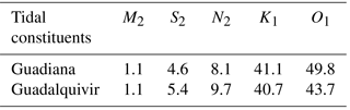
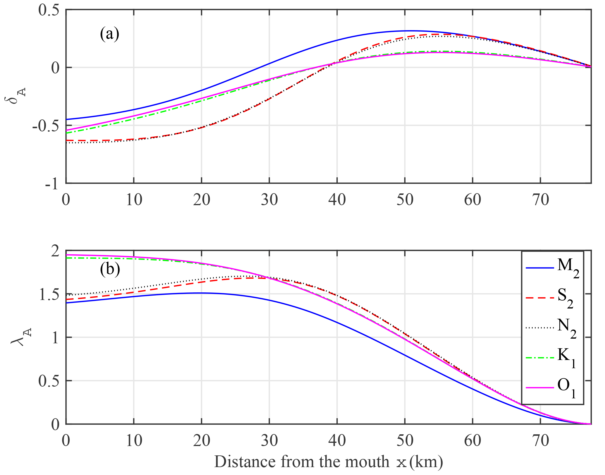
Figure 7Longitudinal variations in tidal damping/amplification number δA (a) and wave celerity number λA (b) for different tidal constituents along the Guadiana estuary.
To understand the tidal dynamics between different tidal constituents along the Guadiana estuary, the longitudinal variations in the tidal damping/amplification number δA and celerity number λA (see their definitions in Table 1) are shown in Fig. 7 where similar minor constituents in semidiurnal (S2, N2) and diurnal (O1, K1) bands behave more or less the same. As shown in Fig. 7a, the minor constituents S2, N2, O1 and K1 experience more friction compared with the predominant M2 tide. Interestingly, we observe a stronger damping (δA<0) of semidiurnal constituents (S2, N2) than of diurnal constituents (O1, K1) in the seaward part of the estuary (around x=0–40 km) although the amplitudes of the diurnal constituents are less than those of the semidiurnal ones. In contrast, the amplification (δA>0) of semidiurnal constituents (S2, N2) is more apparent than those of diurnal constituents (O1, K1) in the landward part of the estuary. For the wave celerity, as expected the dominant M2 tide travels faster (smaller λA) than minor tidal constituents. In addition, we observe that the wave celerity of semidiurnal tidal constituents is larger than those of diurnal constituents in the seaward reach (around x=0–30 km), while it is the opposite in the landward reach, which suggests a complex relation between tidal damping/amplification and wave celerity due to the combined impacts of channel convergence, bottom friction and reflected wave. It is important to note that a standing wave pattern with celerity approaching infinity is produced near the sill due to the superimposition of the incident and reflected waves (see also Garel and Cai, 2018).
For the Guadalquivir estuary, the geometry can be approximated as a converging estuary with a width convergence length of b=65.5 km and a constant stream depth of about 7.1 m. A linear reduction of the storage width ratio of 1.5–1 was adopted over the reach of 0–103 km. The observed tidal amplitudes and phases are best reproduced by using the model for K=46 m1∕3 s−1 (see Fig. 8). In general, the observed tidal properties (tidal amplitude and phase) of different constituents are well reproduced. The enhanced frictional coefficient f for the minor constituents S2, N2, O1 and K1 are 5.4, 9.7, 40.7 and 43.7, respectively (Table 3).
Figure 9 shows the longitudinal variations in tidal damping/amplification and wave celerity for the Guadalquivir estuary, which are similar to those in the Guadiana estuary. In general, we observe that the dominant M2 tide experiences less friction than other secondary semidiurnal tidal constituents although it travels at more or less the same speed in the seaward reach (x=0–35 km). Unlike the Guadiana estuary, the damping experienced by the secondary semidiurnal tides is less than that of diurnal constituents near the estuary mouth (around x=0–7 km; Fig. 9a), while the wave celerity is consistently larger in the seaward reach (x=0–38 km; Fig. 9b). Similar to the Guadiana estuary, we observe that the tidal damping for the secondary semidiurnal tides is stronger than that of diurnal constituents in the central parts of the estuary (around x=7–52 km), whereas their amplifications are larger in the landward part of the estuary although their wave speeds are less.
In particular, the tidal damping along the first half of these two estuaries is mainly due to the damping of the dominant M2 wave owning to the fact that the impact of bottom friction dominates over the channel convergence. Along the upper reach, enhanced morphological convergence and reflection effects (that reduce the overall friction experienced by the propagating wave) result in the overall amplification of the tidal wave. For more details of the tidal hydrodynamics in these two estuaries, readers can refer to Garel and Cai (2018) for the Guadiana estuary and Diez-Minguito et al. (2012) for the Guadalquivir estuary.
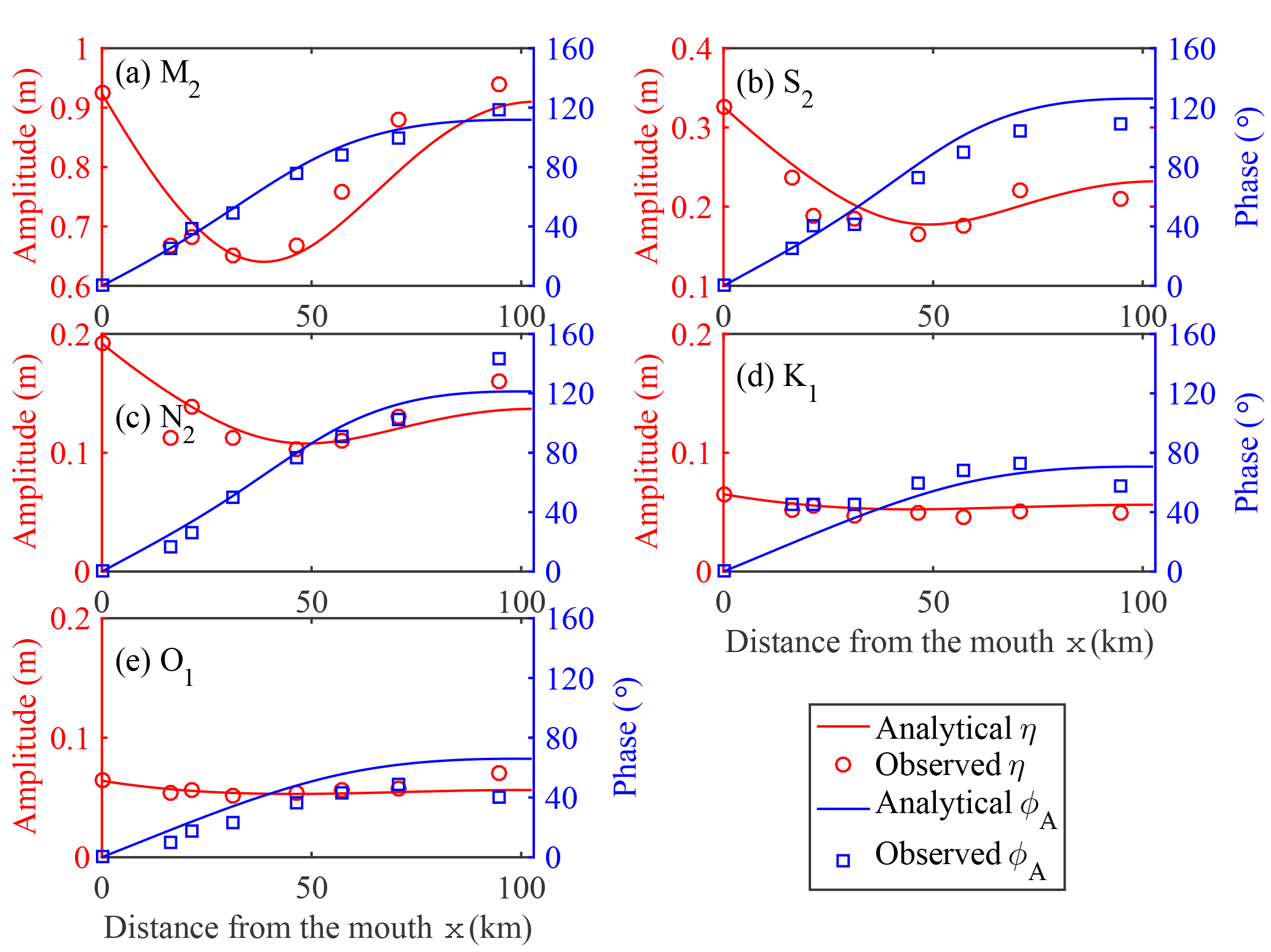
Figure 8Tidal constituents (a) M2, (b) S2, (c) N2, (d) K1 and (e) O1, modeled against observed values of tidal amplitude (m) and phase (∘) of elevation along the Guadalquivir estuary.
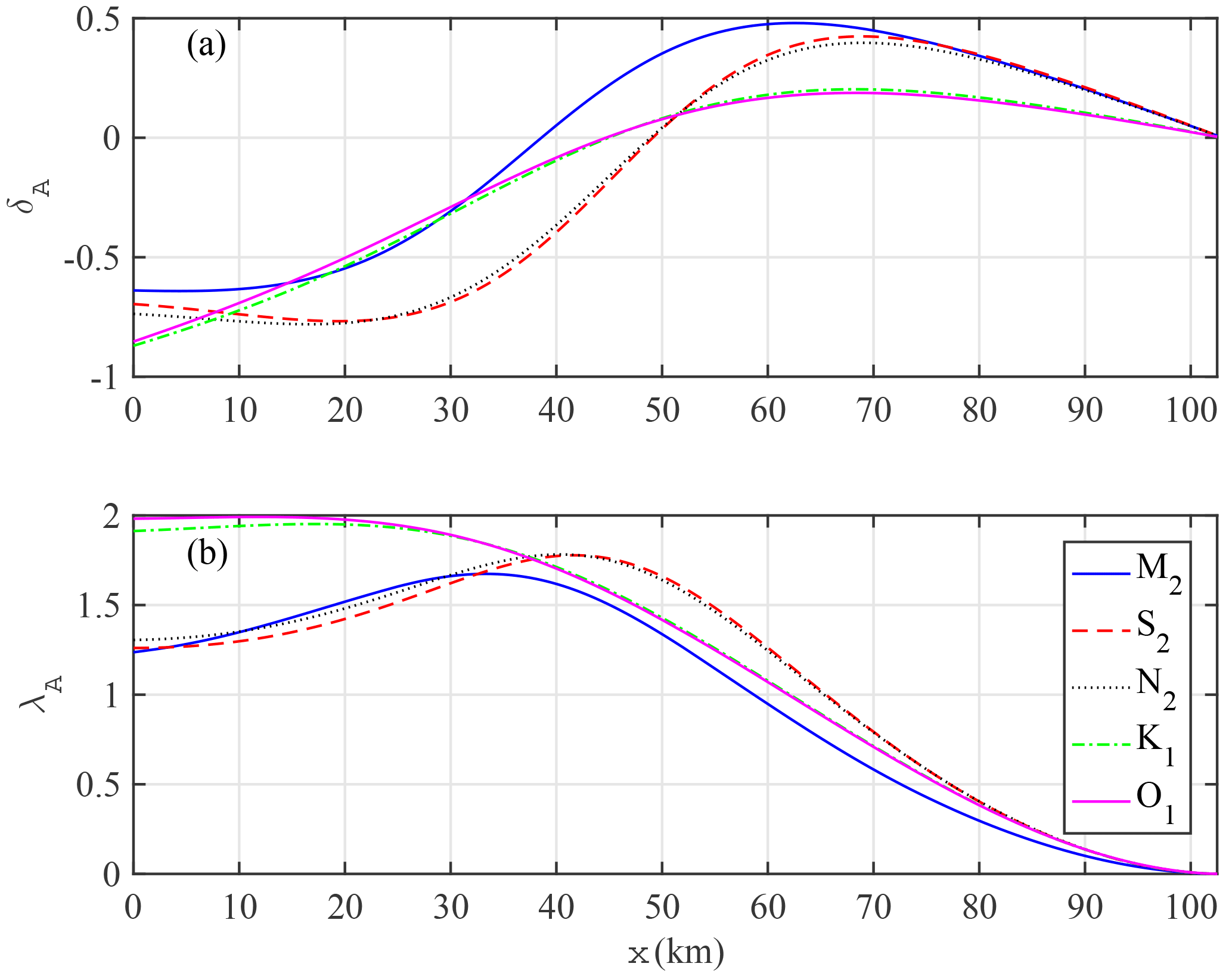
Figure 9Longitudinal variations in tidal damping/amplification number δA (a) and wave celerity number λA (b) for different tidal constituents along the Guadalquivir estuary.
In order to clarify the behavior of different tidal constituents, we present Fig. 10 showing the longitudinal variations in estuary shape number γ (representing the channel convergence) and friction number χn (representing the bottom friction), two major factors determining the tidal hydrodynamics, in both estuaries. Note that the variable estuary shape number γ observed in the Guadalquivir estuary is due to the adoption of a variable storage width ratio rS in the analytical model. On the one hand, the estuary shape numbers for diurnal tides are approximately twice larger than those for semidiurnal tides (Fig. 10a and d) due to the tidal frequency differences (see definition of γ in Table 1). On the other hand, the effective friction experienced by the diurnal tides is much larger than those of the semidiurnal tides due to the mutual interaction between different tidal constituents (Fig. 10b and e, see also Table 3). However, the propagation of different tidal constituents mainly depends on the imbalance between channel convergence and friction, except for those reaches where wave reflection matters (generally close to the head). In particular, in the seaward reach the tidal damping for each tidal constituent can be approximately estimated by (see Eq. 20 by Cai et al., 2012). While the channel convergence effect (represented by γ∕2) is much stronger for diurnal tides than for semidiurnal tides, the frictional effect (represented by χnμcos (ϕ)∕(2λA)) is only slightly larger (Fig. 10c and f). Hence, diurnal tides generally experience relatively less damping in the seaward reach (Figs. 7a and 9a). In the case of the Guadalquivir estuary, diurnal tides are more damped than semidiurnal tides very near the estuary mouth (x=0–7 km). For the second (landward) half of the estuary, the lower amplification experienced by diurnal tides is mainly due to the wave reflection from the closed end (see Garel and Cai, 2018).
The importance of mutual interaction between different tidal constituents is illustrated with the iteratively refined model implemented in both case studies (Figs. 7 and 9). For comparison, Fig. 11 shows the analytically computed damping/amplification number δA and celerity number λA without considering mutual interaction (by setting fn=1 in the model). In this case, the damping experienced by both secondary diurnal and semidiurnal tides is apparently underestimated due to the unrealistic friction adopted in the model (Fig. 11a and c; see also Figs. 7a and 9a). Similarly, the computed wave celerities for secondary tidal constituents are apparently overestimated due to the underestimated bottom friction (Fig. 11b and d; see also Figs. 7b and 9b). To correctly reproduce the main features of different tidal waves, it is required to use the iteratively refined model proposed in this study.
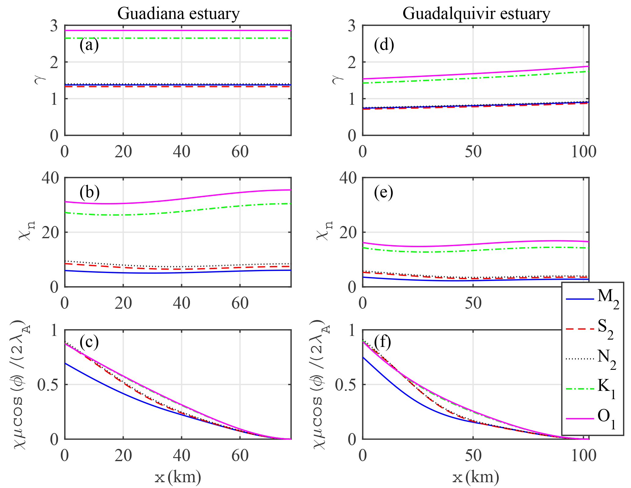
Figure 10Longitudinal variations in estuary shape number γ (a, d), friction number χn (b, e) and χnμcos (ϕ)∕(2λA) (c, f) in the Guadiana estuary (a–c) and Guadalquivir estuary (d–f).
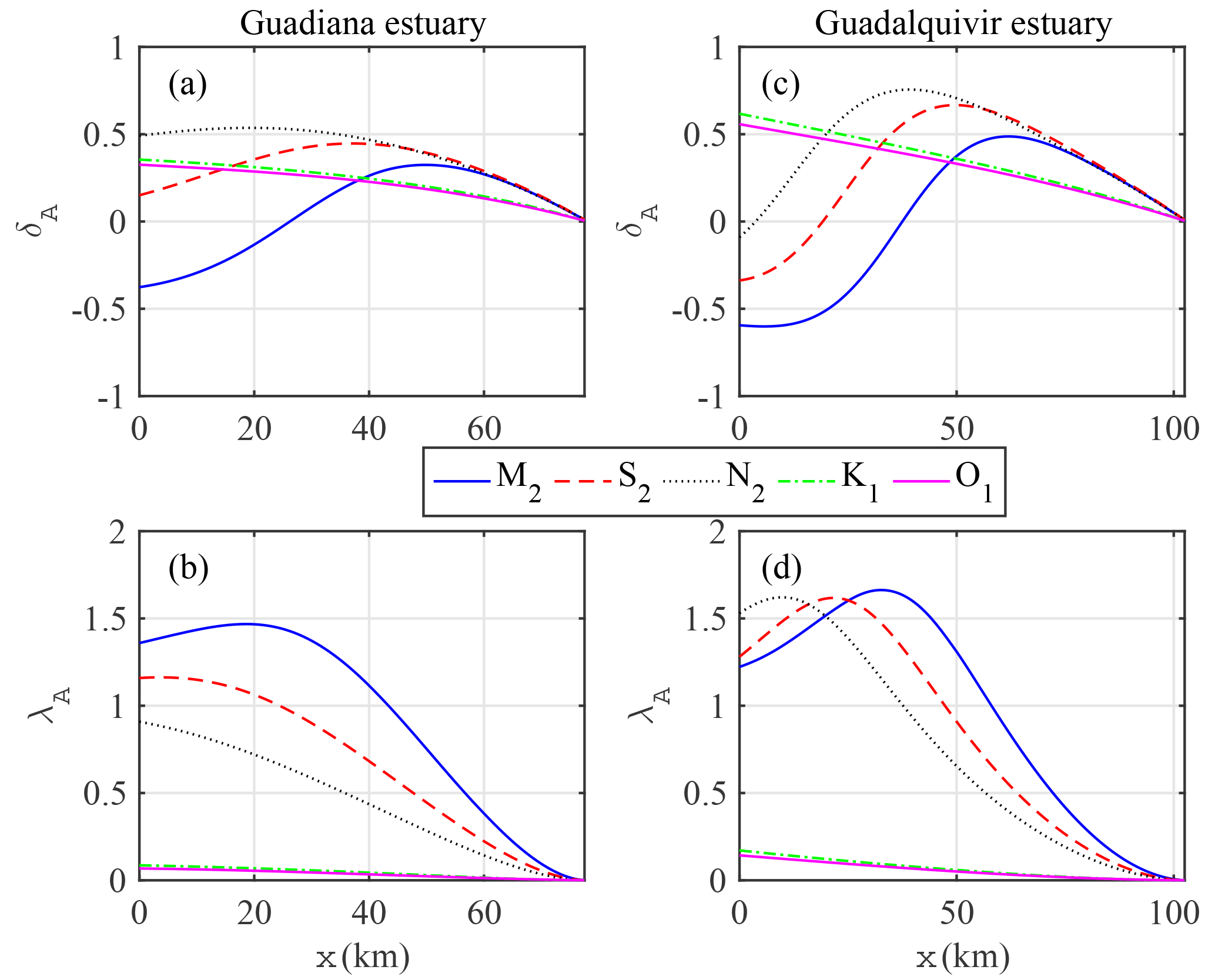
Figure 11Longitudinal variations in damping/amplification number δA (a, c) and celerity number λA (b, d) in the Guadiana estuary (a, b) and Guadalquivir estuary (c, d) in the absence of mutual interaction between different tidal constituents.
In this study, we provide insight into the mutual interactions between one predominant (e.g., M2) and other tidal constituents in estuaries and the role of quadratic friction on tidal wave propagation. An analytical method exploiting Chebyshev polynomials was developed to quantify the effective friction experienced by different tidal constituents. Based on linearization of the quadratic friction, a conceptual model has been used to explore the nonlinear interaction of different tidal constituents, which enables them to be treated independently by means of an iterative procedure. Thus, an analytical hydrodynamic model for a single tidal constituent can be used to reproduce the correct wave behavior for different tidal constituents. In particular, it was shown that a correction of the friction term needs to be used to correctly reproduce the tidal dynamics for minor tidal constituents. The application to the Guadiana and Guadalquivir estuaries shows that the conceptual model can interpret the nonlinear interaction reasonably well when combined with an analytical model for tidal hydrodynamics.
A crucial feature of the proposed approach is the deterministic description of the mutual frictional interaction among tidal constituents, which avoids the need of an independent calibration of the friction parameter for the single constituent. In this respect, further work is required to explore whether a reliable value of the friction coefficient estimated through this method can be parameterized based on observations of the bottom roughness of the estuary.
The data and source codes used to reproduce the experiments presented in this paper are available from the authors upon request (egarel@ualg.pt).
In this paper, analytical solutions for a semi-closed estuary proposed by Toffolon and Savenije (2011) were used to reproduce the longitudinal tidal dynamics along the estuary axis. The solution makes use of the parameters that are defined in Table 1.
The analytical solutions for the tidal wave amplitudes and phases are given by
where ℜ and ℑ are the real and imaginary parts of the corresponding term, and A* and V* are unknown complex functions varying along the dimensionless coordinate :
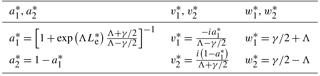
For a tidal channel with a closed end, the analytical solutions for the unknown variables in Eqs. (A1) and (A1) are listed in Table A1, where Λ is a complex variable, defined as
where the coefficient 8∕(3π) stems from the adoption of Lorentz's linearization when considering only one single predominant tidal constituent (e.g., M2).
Since the friction parameter depends on the unknown value of μ (or υ), an iterative procedure was used to determine the correct wave behavior. In addition, to account for the longitudinal variation in the cross section (e.g., estuary depth), a multi-reach technique was adopted by subdividing the entire estuary into multiple sub-reaches; the solutions were obtained by solving a set of linear equations with internal boundary conditions at the junction of the sub-reaches satisfying the continuity condition (see details in Toffolon and Savenije, 2011).
For given computed values of A* and V*, the dependent parameters defined in Table 1 can be computed using the following equations:
Table A1Analytical expressions for unknown complex variables for the case of a closed estuary.
The following trigonometric equation
is used to convert the third-order terms of Eq. (5) to the harmonic constituents. For a single harmonic, it follows that
For two harmonic constituents, the Chebyshev polynomials approximation of is expressed as
In Eq. (B3), the cubic term can be expanded as
Making use of the trigonometric equations to expand the power of the cosine functions (e.g., cos 3(ω1t) and cos 2(ω1t)) and extracting only the harmonic terms with frequencies ω1 and ω2, Eq. (B3) can be reduced to Eq. (9).
For the case of many constituents, here we only provide the exact coefficients for n=3:
Equations (B3) to (B3) reduce to Eqs. (10) and (10) when ε3=0 (i.e., υ3=0).
The supplement related to this article is available online at: https://doi.org/10.5194/os-14-769-2018-supplement.
HC and EG conceived the study and wrote the draft of the paper. MT, HHGS and QY contributed to the improvement of the paper. All authors reviewed the paper.
The authors declare that they have no conflict of interest.
We acknowledge the financial support from the National Key R & D of China
(grant no. 2016YFC0402600), from the National Natural Science Foundation of
China (grant no. 51709287), from the Basic Research Program of Sun Yat-Sen
University (grant no. 17lgzd12), and from the Water Resource Science and
Technology Innovation Program of Guangdong Province (grant no. 2016-20). The
work of Erwan Garel was supported by FCT research contract IF/00661/2014/CP1234.
Edited by: John M. Huthnance
Reviewed by: David Bowers and Job Dronkers
Cai, H., Savenije, H. H. G., and Toffolon, M.: A new analytical framework for assessing the effect of sea-level rise and dredging on tidal damping in estuaries, J. Geophys. Res., 117, C09023, https://doi.org/10.1029/2012JC008000, 2012. a
Cai, H., Toffolon, M., and Savenije, H. H. G.: Analytical investigation of superposition between predominant M2 and other tidal constituents in estuaries, in: Proceedings of 36th IAHR World Congress, Delft – The Hague, 2015. a, b
Cai, H., Toffolon, M., and Savenije, H. H. G.: An Analytical Approach to Determining Resonance in Semi-Closed Convergent Tidal Channels, Coast Eng. J., 58, 1650009, https://doi.org/10.1142/S0578563416500091, 2016. a
Diez-Minguito, M., Baquerizo, A., Ortega-Sanchez, M., Navarro, G., and Losada, M. A.: Tide transformation in the Guadalquivir estuary (SW Spain) and process-based zonation, J. Geophys. Res., 117, C03019, https://doi.org/10.1029/2011jc007344, 2012. a, b, c, d
Doodson, A. T.: Perturbations of Harmonic Tidal Constants, in: vol. 106 of 739, Proceedings of the Royal Society, London, 513–526, 1924. a
Dronkers, J. J.: Tidal computations in River and Coastal Waters, Elsevier, New York, 1964. a, b, c
Fang, G.: Nonlinear effects of tidal friction, Acta Oceanol. Sin., 6, 105–122, 1987. a, b, c, d
Garel, E.: Guadiana River estuary – Investigating the past, present and future, in: Present Dynamics of the Guadiana Estuary, edited by: Moura, D., Gomes, A., Mendes, I., and Anibal, J., University of Algarve, Faro, Portugal, 15–37, 2017. a, b, c
Garel, E. and Cai, H.: Effects of Tidal-Forcing Variations on Tidal Properties Along a Narrow Convergent Estuary, Estuar. Coast, https://doi.org/10.1007/s12237-018-0410-y, in press, 2018. a, b, c
Garel, E. and Ferreira, O.: Fortnightly changes in water transport direction across the mouth of a narrow estuary, Estuar. Coast, 36, 286–299, https://doi.org/10.1007/s12237-012-9566-z, 2013. a
Garel, E., Pinto, L., Santos, A., and Ferreira, O.: Tidal and river discharge forcing upon water and sediment circulation at a rock-bound estuary (Guadiana estuary, Portugal), Estuar. Coast. Shelf S., 84, 269–281, https://doi.org/10.1016/j.ecss.2009.07.002, 2009. a
Godin, G.: Compact Approximations to the Bottom Friction Term, for the Study of Tides Propagating in Channels, Cont. Shelf Res., 11, 579–589, https://doi.org/10.1016/0278-4343(91)90013-V, 1991. a, b, c, d, e
Godin, G.: The propagation of tides up rivers with special considerations on the upper Saint Lawrence river, Estuar. Coast. Shelf S., 48, 307–324, https://doi.org/10.1006/ecss.1998.0422, 1999. a, b, c, d, e, f
Heaps, N. S.: Linearized vertically-integrated equation for residual circulation in coastal seas, Dtsch. Hydrogr. Z., 31, 147–169, https://doi.org/10.1007/BF02224467, 1978. a
Inoue, R. and Garrett, C.: Fourier representation of quadratic friction, J. Phys. Oceanogr., 37, 593–610, https://doi.org/10.1175/Jpo2999.1, 2007. a, b, c, d, e
Jeffreys, H.: The Earth: Its Origin, History and Physical Constitution, 5th Edn., Cambridge University Press, Cambridge, UK, 1970. a
Kabbaj, A. and Le Provost, C.: Nonlinear tidal waves in channels: a perturbation method adapted to the importance of quadratic bottom friction, Tellus, 32, 143–163, https://doi.org/10.1111/j.2153-3490.1980.tb00942.x, 1980. a
Le Provost, C.: Décomposition spectrale du terme quadratique de frottement dans les équations des marées littorales, C. R. Acad. Sci. Paris, 276, 653–656, 1973. a, b, c, d
Le Provost, C.: Generation of Overtides and compound tides (review), in: Tidal Hydrodynamics, edited by: Parker, B., John Wiley and Sons, Hoboken, NJ, 269–295, 1991. a
Le Provost, C. and Fornerino, M.: Tidal spectroscopy of the English Channel with a numerical model, J. Phys. Oceanogr., 15, 1009–1031, https://doi.org/10.1175/1520-0485(1985)015<1008:TSOTEC>2.0.CO;2, 1985. a
Le Provost, C., Rougier, G., and Poncet, A.: Numerical modeling of the harmonic constituents of the tides, with application to the English Channel, J. Phys. Oceanogr., 11, 1123–1138, https://doi.org/10.1175/1520-0485(1981)011<1123:NMOTHC>2.0.CO;2, 1981. a
Lorentz, H. A.: Verslag Staatscommissie Zuiderzee, Tech. rep., Algemene Landsdrukkerij, the Hague, the Netherlands, 1926. a
Molines, J. M., Fornerino, M., and Le Provost, C.: Tidal spectroscopy of a coastal area: observed and simulated tides of the Lake Maracaibo system, Cont. Shelf Res., 9, 301–323, https://doi.org/10.1016/0278-4343(89)90036-8, 1989. a
Parker, B. B.: The relative importance of the various nonlinear mechanisms in a wide range of tidal interactions, in: Tidal Hydrodynamics, edited by: Parker, B., John Wiley and Sons, Hoboken, NJ, 237–268, 1991. a
Pawlowicz, R., Beardsley, B., and Lentz, S.: Classical tidal harmonic analysis including error estimates in MATLAB using T-TIDE, Comput. Geosci., 28, 929–937, https://doi.org/10.1016/S0098-3004(02)00013-4, 2002. a
Pingree, R. D.: Spring Tides and Quadratic Friction, Deep-Sea Res. Pt. A, 30, 929–944, https://doi.org/10.1016/0198-0149(83)90049-3, 1983. a, b, c, d, e
Prandle, D.: The influence of bed friction and vertical eddy viscosity on tidal propagation, Cont. Shelf Res., 17, 1367–1374, https://doi.org/10.1016/S0278-4343(97)00013-7, 1997. a
Proudman, J.: Dynamical oceanography, Methuen, London, 1953. a, b
Savenije, H. H. G., Toffolon, M., Haas, J., and Veling, E. J. M.: Analytical description of tidal dynamics in convergent estuaries, J. Geophys. Res., 113, C10025, https://doi.org/10.1029/2007JC004408, 2008. a
Schuttelaars, H. M., de Jonge, V. N., and Chernetsky, A.: Improving the predictive power when modelling physical effects of human interventions in estuarine systems, Ocean Coast. Manage., 79, 70–82, https://doi.org/10.1016/j.ocecoaman.2012.05.009, 2013. a
Toffolon, M. and Savenije, H. H. G.: Revisiting linearized one-dimensional tidal propagation, J. Geophys. Res., 116, C07007, https://doi.org/10.1029/2010JC006616, 2011. a, b, c, d
Winterwerp, J. C., Wang, Z. B., van Braeckel, A., van Holland, G., and Kosters, F.: Man-induced regime shifts in small estuaries – II: a comparison of rivers, Ocean Dynam., 63, 1293–1306, https://doi.org/10.1007/s10236-013-0663-8, 2013. a
- Abstract
- Introduction
- Materials and methods
- Conceptual model
- Results
- Conclusions
- Data availability
- Appendix A: Analytical solutions of tidal hydrodynamics for a single tidal constituent
- Appendix B: Coefficients of the Godin's expansion
- Author contributions
- Competing interests
- Acknowledgements
- References
- Supplement