Ocean circulation, sea ice, and productivity simulated in Jones Sound, Canadian Arctic Archipelago, between 2003–2016

Jones Sound is one of three critical waterways in the Canadian Arctic Archipelago that regulate liquid exchange between the Arctic Ocean and northern Atlantic Ocean. However, to date, no high-resolution ocean circulation model exists to study the recent evolution of Jones Sound, meaning that our understanding of circulation within the sound is based either on temporally and spatially sparse oceanographic observations or on extrapolating conditions within Baffin Bay, which has a more dense observational record. To address this, we develop a high-resolution ($\mathrm{1}/\mathrm{120}$°, 0.9 km) Jones Sound configuration of the Massachusetts Institute of Technology general circulation model and perform coupled ocean–sea ice–biological productivity simulations between 2003–2016. We find that circulation through Lady Ann Strait, Fram Sound, and Glacier Strait comprises 71 %, 14 %, and 15 % of the volumetric transport into and out of Jones Sound, with tidal flushing enhancing the magnitude of volumetric transport through Fram Sound. Warming Atlantic Water within western Baffin Bay flows into Jones Sound through Lady Ann Strait, becomes well-mixed, and circulates counterclockwise, encroaching on the terminus of most tidewater glaciers that line the eastern periphery of the sound. Furthermore, we find that sustained atmospheric and oceanic warming drives an 11 % reduction in the 2003–2016 mean summertime sea ice area, decreased wintertime sea ice thickness, and delayed onset of sea ice refreeze in the fall (thus lengthening the amount of time during which Jones Sound is ice-free). Tidal flushing through Cardigan Strait is critical in triggering melt-back of sea ice across northern Jones Sound. Lastly, this decline in sea ice increases light availability and, when coupled with warming of the subsurface waters in Jones Sound, facilitates enhanced primary productivity down to ∼ 21 m depth. While we note that the modeled warming signal in Baffin Bay is overestimated relative to observations, the results presented here improve our general understanding of how this critical waterway might change under continued polar-amplified global warming and underscores the need for sustained oceanographic observations in this region.

1 Introduction

The Canadian Arctic Archipelago (CAA) is a tangle of shallow basins and narrow straits that connect the Arctic Ocean to the northern Atlantic Ocean. Flow through the CAA has been found to be primarily controlled by the baroclinic gradient that exists between the Beaufort Gyre and northern Baffin Bay (Kliem and Greenberg, 2003; Prinsenberg and Bennett, 1987; Wang et al., 2017; Wekerle et al., 2013), with high-frequency variability driven by the wind (Peterson et al., 2012). The Queen Elizabeth Islands (QEIs) in the north make up an area with relatively small islands surrounded by the larger Ellesmere, Devon, Cornwallis, Bathurst, Melville, and Prince Patrick islands. Arctic Ocean waters flow through the QEIs and are transported into northern Baffin Bay (and eventually the North Atlantic Ocean) through three main passageways: Lancaster Sound, Nares Strait, and Jones Sound. Within these waterways, moorings reveal a mean transport of 0.46 Sv (1 Sv is equal to 10⁶ m³ s⁻¹) in western Lancaster Sound between 1998–2010 (Peterson et al., 2012; Prinsenberg and Hamilton, 2005), 0.71±0.09 and 1.03±0.11 Sv between 2003 and 2006 and between 2007 and 2009, respectively, along Nares Strait (Munchow and Humfrey, 2008; Münchow, 2016), and 0.3 Sv between 1998–2002 flowing through Jones Sound (Melling et al., 2008). Thus, the rough balance of transport through these three main passages is 46 % Nares Strait, 34 % Lancaster Sound, and 20 % Jones Sound (Melling et al., 2008; Grivault et al., 2018).

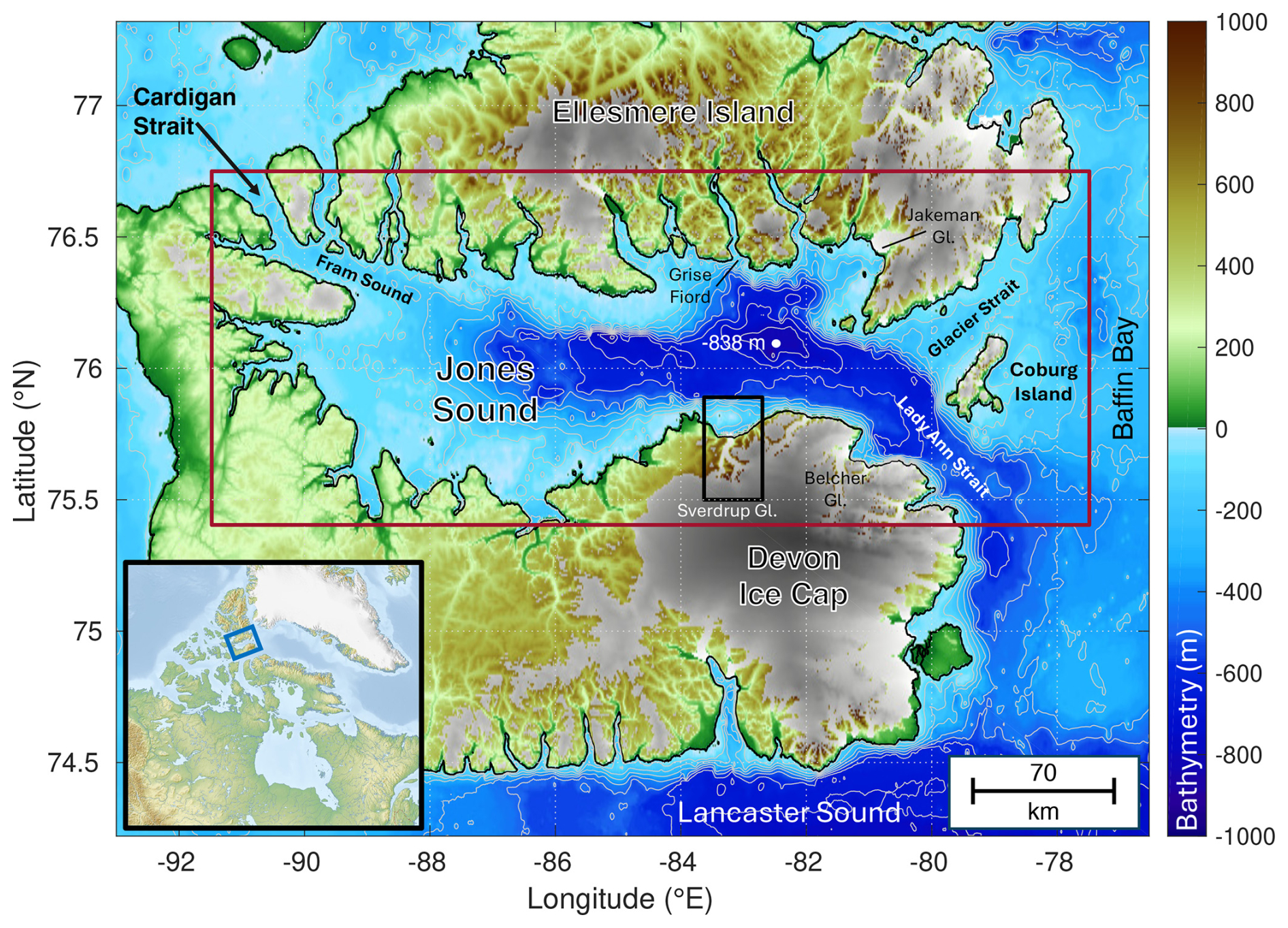
Figure 1 Domain featuring ocean bathymetry (m) from the SRTM15+ dataset (Tozer et al., 2019), where blue shading denotes bathymetry below sea level. Gray shading denotes the present-day extent of land ice, the red box denotes the domain of the high-resolution ocean circulation model, and the black box denotes where new bathymetry observations were implemented in the ocean model in Brae Bay. Geographic features mentioned in the text are labeled, including glaciers, waterways, and islands.

Jones Sound is home to the Inuit hamlet of Ausuiktuq (Grise Fiord) and is a marine region surrounded by glaciers draining large ice fields and ice caps on both the Ellesmere Island and Devon Island. It is the third largest export pathway in the CAA (Grivault et al., 2018; Melling et al., 2008; Zhang et al., 2016), connecting directly to the Arctic Ocean at the narrow (15 km) and shallow (150 m) western gateways of Hell Gates/Cardigan Strait (which merge into Fram Sound) and exchanging with Baffin Bay on the east side of the sound at a depth of 450 m (Fig. 1). The western half of Jones Sound is shallow, being ∼ 200 m depth, while the eastern basin is deeper, having a maximum depth of ∼ 840 m and greater exchange with external waterways. Aside from facilitating liquid exchange between the Arctic Ocean and northern Atlantic Ocean, Jones Sound also hosts a diverse biological ecosystem that is sustained in part by ice–ocean interactions of tidewater glacier termini as well as seasonally varying ocean and sea ice conditions (Bhatia et al., 2021). However, as part of the broader Arctic, Jones Sound is vulnerable to changing climate conditions that threaten these natural resources. For instance, Gardner et al. (2012) found that ice mass loss across the QEIs tripled from 31±8 Gt yr⁻¹ in 2004–2006 to 92±12 Gt yr⁻¹ in 2007–2009, largely driven by Arctic-amplified atmospheric warming that outpaces the global average by 3 times. Below the halocline within the Baffin Bay, mid-depth Atlantic Water (AW) that penetrates into the CAA and Arctic Ocean has been warming steadily since at least the early 2000s (Polyakov et al., 2013; Wang et al., 2020; Ballinger et al., 2022). This atmospheric and oceanic warming has also driven recent declines in sea ice extent, with the summer sea ice area in northern Canadian waters and Baffin Bay declining at a rate of 7.1 % per decade and 11.6 % per decade, respectively (Tivy et al., 2011). Given that sea ice serves as hunting platforms for polar bears, resting grounds and nursery areas for walruses and seals, and hosts for algae that grow on the ice base, these reductions in sea ice have cascading impacts on marine ecosystems.

The maze of islands, narrow straits, complex coastlines, and shallow bathymetry complicates ocean circulation, sea ice, and biological productivity modeling in the CAA. However, numerical modeling remains the best way to begin understanding how these critical environments, as well as their joint interactions, have been changing. Recent ocean modeling studies are largely capable of resolving mean transport through Lancaster Sound and Nares Strait (McGeehan and Maslowski, 2012; Shroyer et al., 2015; Wang et al., 2017; Wekerle et al., 2013; Zhang et al., 2016); however, coarse horizontal meshes cause issues with resolving baroclinic flow in narrower channels, such as Fram Sound, leading to large uncertainty in volume estimates into and general circulation within Jones Sound. This, in turn, limits the fidelity of sea ice and productivity models in this region. To address this, we develop a high-resolution Jones Sound configuration of the Massachusetts Institute of Technology general circulation model and perform coupled ocean–sea ice–biological productivity simulations between 2003–2016 to investigate the following: (1) the magnitude and spatial/temporal distribution of volumetric transport into and out of Jones Sound, (2) fine-scale circulation features within Jones Sound and their impact on water column structure on seasonal timescales, (3) seasonal and decadal variations in sea ice dynamics, and (4) the impact of simulated changes in ocean and sea ice conditions on productivity within Jones Sound. By investigating these four topics, we seek to improve our understanding of circulation, sea ice dynamics, and productivity within Jones Sound and how it fits within the broader context of the Canadian Arctic Archipelago. Below, we provide information on the setup of the numerical ocean, sea ice, and biogeochemical model as well as an overview of the simulations.

2 Methods

Here, we provide information on the setup of the ocean, sea ice, and biogeochemical model that we use to simulate circulation in Jones Sound between 2003–2016. We note that we first developed a low-resolution ocean–sea ice model to simulate the region surrounding Jones Sound between 2002–2016 (from here on referred to as the “low-resolution simulation”), from which we extract initial and boundary conditions to force our high-resolution ocean–sea ice–productivity simulation of Jones Sound between 2003–2016 (hereon referred to as the “high-resolution simulation”). Most of the model setup between the two simulations is identical aside from the source of the boundary and initial conditions as well as the domain extent and resolution.

2.1 Ocean model setup

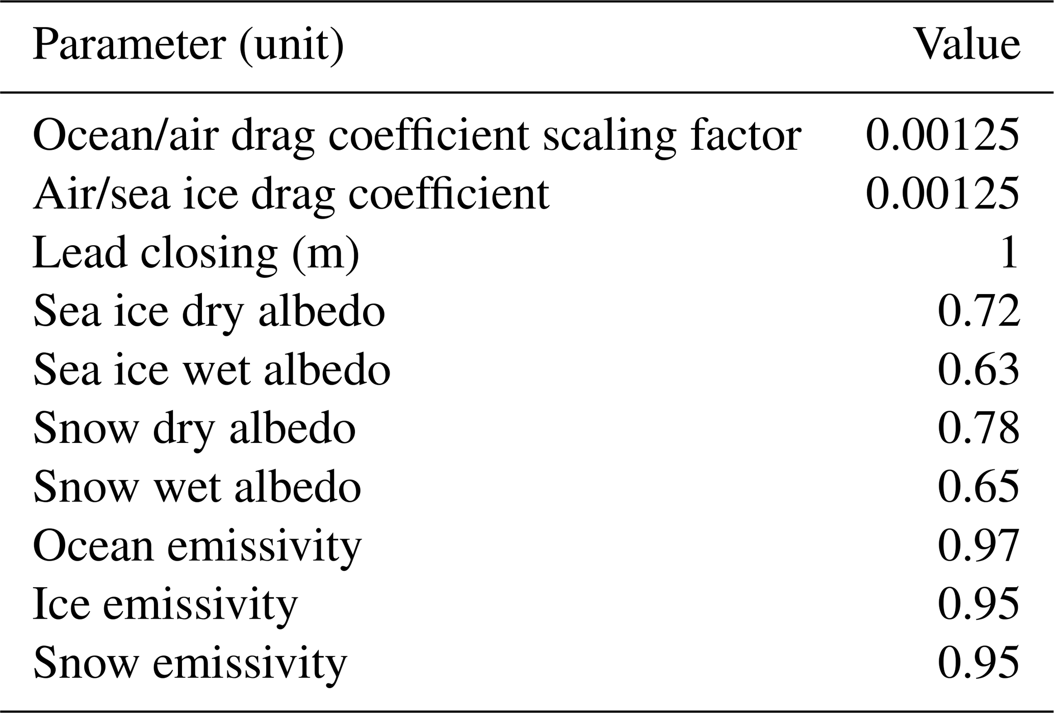
We model ocean circulation using a regional Canadian Arctic configuration of the ocean component of the Massachusetts Institute of Technology general circulation model (MITgcm; Marshall et al., 1997). This includes use of the hydrostatic approximation, a dynamic/thermodynamic model to simulate sea ice dynamics (Losch et al., 2010), and the Biogeochemistry with Light, Iron, Nutrients, and Gases with Nitrogen (N-BLING) productivity module to simulate photosynthetic biological productivity (only used in the high-resolution simulation and described in Sect. 2.2; Galbraith et al., 2010). The low-resolution simulation domain extends from 73.25–76.75° N and 74–91.5° E, has a nominal horizontal resolution of $\mathrm{1}/\mathrm{24}$° (∼ 5 km), and contains 70 vertical levels (with a vertical resolution of 7 m through 266 m depth, then decreasing to a minimum resolution of 62 m at the lowest ocean level; 1090 m). The high-resolution simulation domain extends from 75.40 to 76.70° N and from −77.45 to −91.45° E (red outline in Fig. 1), has a nominal horizontal resolution of $\mathrm{1}/\mathrm{120}$° (∼ 900 m), and contains 70 vertical levels (with a vertical resolution of 7 m through 266 m depth, then decreasing to a minimum resolution of 56 m at the lowest depth of 963 m). Model bathymetry is based on the SRTM15+ digital elevation model (Tozer et al., 2019) with corrections applied in Brae Bay (black box near Sverdrup Glacier in Fig. 1) and the oceanic regions near Grise Fiord following multibeam and point measurements. Ocean and sea ice parameter values that differ from Nakayama et al. (2018) are provided in Table 1.

Initial and boundary conditions for the low-resolution ocean simulation are extracted from the $\mathrm{1}/\mathrm{12}$° Arctic and Northern Hemisphere Atlantic (ANHA12) configuration of the NEMO model that covers the entire North Atlantic Ocean down to 20° S and was run from 2002–2018 (Hu et al., 2019; Gillard et al., 2020). Fields used as initial and boundary conditions in our ocean simulations include temperature, salinity, the zonal (u) and meridional (v) velocity components, and sea surface height. In addition, fields used to initialize and drive the sea ice model include sea ice area, thickness, snow content, salt content, and the u and v sea ice velocity components. Initial conditions were extracted at model date 1 January 2002 and boundary conditions are extracted monthly through 31 December 2016. Initial and bimonthly boundary conditions in the high-resolution simulation are extracted from the low-resolution simulation, with an initialization date of 1 January 2003.

Atmospheric forcing is taken in 3 h intervals from the Arctic System Reanalysis version 2 (ASRv2; Bromwich et al., 2018) and interpolated onto the model grids. We use the following variables: 2 m air temperature, 2 m specific humidity, precipitation, 10 m u and v wind components, shortwave and longwave radiation, atmospheric pressure, evaporation, and river/glacial runoff. The time series of all atmospheric forcing fields are shown in Fig. 2. In addition, tidal forcing (amplitude and phase) is prescribed in the high-resolution simulation using the Arctic 2 kilometer Tide Model (Arc2kmTM; Howard and Padman, 2021) and includes the following constituents: M₂, S₂, N₂, K₂, K₁, O₁, P₁, and Q₁. In MITgcm, tidal forcing is applied along the ocean model boundaries as a surface elevation perturbation and as barotropic flow that propagates throughout the domain.

Table 1 MITgcm ocean and sea ice model parameters and values used in this study. Only parameters that are different from Nakayama et al. (2018) are shown.

2.2 N-BLING setup

The Nitrogen version of the Biogeochemistry with Light, Iron, Nutrients, and Gases (N-BLING) productivity module simulates biogeochemical cycling of key elements/micronutrients as well as photosynthetic productivity and has been implemented in MITgcm as a module (Galbraith et al., 2010; Verdy and Mazloff, 2017). N-BLING is driven by the physical ocean model as well as atmospheric carbon dioxide concentrations, which are taken monthly between 2003–2016 from a meteorological station in Alert, Canada, and assumed to be spatially uniform across our high-resolution domain. Incoming solar radiation, taken from ASRv2, also drives N-BLING. Initial and monthly boundary conditions for N-BLING include the following: dissolved inorganic carbon (DIC) and alkalinity taken from the Global Ocean Data Analysis Project version 2 (GLODAPv2; Olsen et al., 2016); O₂, NO₃, PO₄, and silica taken from the World Ocean Atlas (WOA; Garcia et al., 2018); Fe, dissolved organic nitrogen, dissolved organic phosphorus, and initial small/large/diazotroph phytoplankton from a global run of BLINGv2 (Eric Galbraith, personal communication, 2023); and iron dust deposition from Mahowald et al. (2005). N-BLING runs on the same computational grid and time step as the ocean model and coupling is only one-way, meaning that N-BLING-simulated productivity does not influence the radiative fluxes and thus the ocean circulation and sea ice growth.

2.3 Model runs

We first run the low-resolution ocean–sea ice simulation between 1 January 2002 and 31 December 2016 using a baroclinic time step of 120 s. From the low-resolution simulation, we extract initial and boundary conditions to force the high-resolution ocean–sea ice–biological productivity simulation, which is run between 1 January 2003 and 31 December 2016 using a baroclinic time step of 70 s. We performed simulations that do and do not resolve tidal forcing to explore the impact of tides on ocean circulation and sea ice productivity in Jones Sound (see Appendix A). All results discussed below are taken from the high-resolution simulation. We note that N-BLING crashed in May 2015, so we only report productivity results up to then. We describe the cause of this crash in the Discussion section.

3 Results

3.1 Model forcing

Between 2002–2016, large trends exist in atmospheric forcing variables in ASRv2 over Jones Sound. The time series of all atmospheric forcing variables are shown in Fig. 2, where domain-wide means are taken except for evaporation, precipitation, and runoff, which are integrated across the domain. In panels (a)–(i), we overlay the overall and summer linear trends as colored solid and dotted lines, respectively, and report the total trend in the title of each panel. In panel (j), we show trend lines on variables that have been normalized. Overall, we find strong increasing trends in the 2 m air temperature, which is increasing at an overall rate of 0.87 °C per decade and a summer rate of 1.19 °C per decade (1.37 times higher than the overall trend). This strong surface warming trend drives strong positive trends in summer relative humidity ($\mathrm{3.76}\times {\mathrm{10}}^{-\mathrm{4}}$ kg kg⁻¹ per decade, 2.81 times stronger than the overall relative humidity trend), summer and overall evaporation, and summer runoff ($\mathrm{6.583}\times {\mathrm{10}}^{-\mathrm{4}}$ m s⁻¹ per decade). We see minimal changes in mean atmospheric pressure, mean shortwave and longwave radiation, mean 2 m wind speed, and total integrated precipitation.

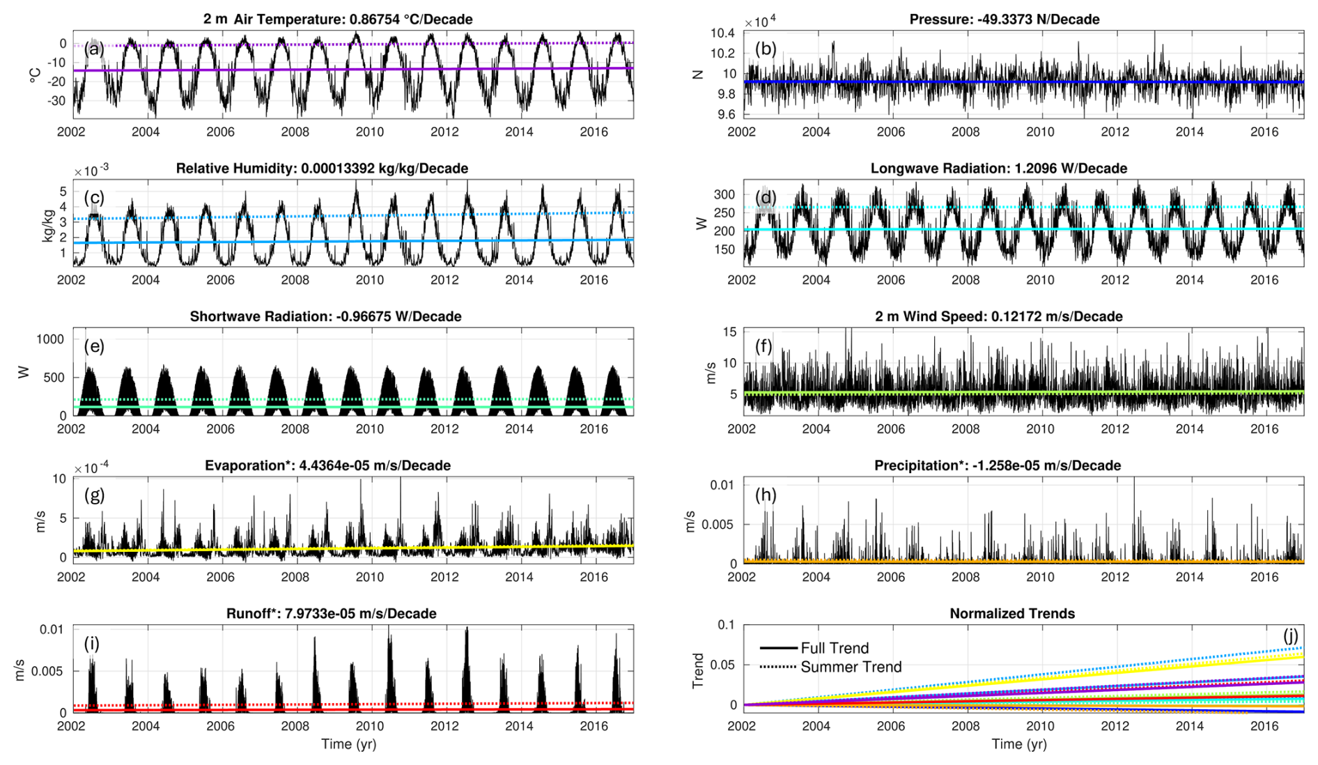
Figure 2 Time series of ASRv2 (a) 2 m air temperature, (b) surface atmospheric pressure, (c) relative humidity, (d) downward longwave radiation, (e) downward shortwave radiation, (f) 2 m wind speed, (g) evaporation, (h) precipitation, and (i) runoff. Panels (a)–(f) show domain-wide averages, while (g)–(i) (names appended with ^*) show sums integrated across the domain. In each panel, the best-fit lines for all data (solid colored line) and for summer data (dotted colored line) are overlaid, and the slope of the all-data line (per decade) is included in the title. Panel (j) plots all best-fit lines computed on data that have been normalized. The lines are then vertically shifted so that the initial value is 0 to facilitate trend comparison.

Along the ocean model boundaries, we find large changes in the ocean state between 2002 and 2016 as simulated by the ANHA12 configuration of NEMO, from which we extract our ocean boundary conditions. Figure A1 in Appendix A1 shows vertical profiles of ocean potential temperature applied to the eastern boundary (−74° W) of the low-resolution ocean simulation in January of 2002, 2007, 2012, and 2016. A strong warming signal of the winter mid-depth Atlantic Water (between 100–300 m depth) is evident after 2007, where waters warm by over 2 °C in ∼ 10 years in this simulation. We note that this simulated warming signal of the Atlantic Water is overestimated, as oceanic observations taken on the Arcticnet Amundsen icebreaker report 1–1.5 °C of warming of this water mass in northern Baffin Bay over this same time period. We discuss the implications of this overestimated ocean warming in the Discussion section.

3.2 Model evaluation

We evaluate our coupled ocean–sea ice model of Jones Sound against repeat summertime casts of conductivity, temperature, and depth (CTD) ocean sensors made aboard the Amundsen icebreaker between 2005 and 2021 (Amundsen Science Data Collection, 2003–2021). We selected five sample sites based on data availability within our model domain: two locations spanning longitudinally across northern Baffin Bay, one site in the center of the eastern entrance of Lancaster Sound, one site close to Belcher Glacier, and one site near the center of Jones Sound. Observed and modeled temperature profiles are plotted in Fig. 3a, c, e, and g and in panels b, d, f, and h, respectively (solid and dotted lines, respectively). The color of the profile is associated with the year it was taken. Note that gray solid profiles indicate observed profiles taken after 2016 and dotted gray profiles were extracted in summer 2016. We included these profiles because the only currently publicly available CTD casts within Jones Sound in this dataset were taken in 2019 and 2021. The brown line in panel (g) was measured in the summer of 2019 by Bhatia et al. (2021). Note that we also present an evaluation of salinity profiles in Appendix A1 (Fig. A2).

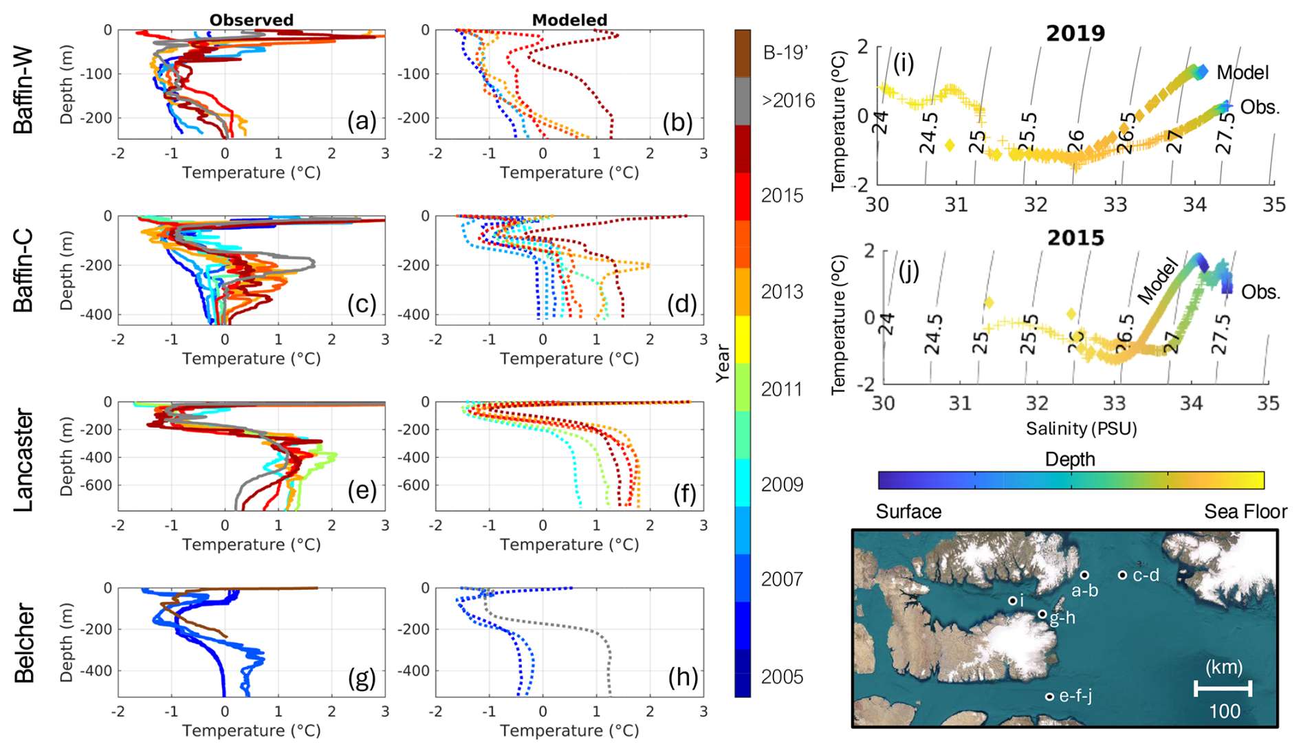
Figure 3 Comparison of observed (a, c, e, g, solid lines) and modeled (b, d, f, h, dotted lines) ocean temperature vertical profiles taken in western Baffin Bay (a–b), in central Baffin Bay (c–d), at the eastern entrance of Lancaster Sound (e–f), and near Belcher Glacier (g–h). The color of the line indicates the year of the profile, and gray denotes any profile taken after 2016. Observations are summertime CTD rosettes taken aboard the Amundsen icebreaker (Amundsen Science Data Collection, 2003–2021), and the brown line in (b) is a profile from Bhatia et al. (2021) that was taken in summer 2019 (B-19'). (i–j) Temperature–salinity plots taken in (i) 2019 in Jones Sound and (j) 2015 in the eastern entrance of Lancaster Sound. The color of the marker corresponds to the depth. The observed and modeled profiles are labeled.

In the profiles taken across northern Baffin Bay and in Lancaster Sound (Fig. 3a–f), we find that our model is generally able to replicate the summertime thermal properties of the ocean in these sample locations. In particular, we properly model the depth of the thermocline (located between 100–300 m depth) and mid-depth Atlantic Water temperatures at all sample sites. One notable exception to this is a warm bias in the modeled seabed ocean temperatures in the sample site in northern Baffin Bay (Fig. 3c–d), where observed ocean temperatures increase from −0.5 to −1 °C between 2005–2016 but modeled ocean temperatures increase from 0 to 1.5 °C during this same time period. That is, we overestimate warming of the bottom ocean water in Baffin Bay but reasonably match warming of the mid-depth Atlantic Water in the summer. We expect that this overestimated bottom ocean warming stems from the overestimated warming in our NEMO-derived boundary conditions (Fig. A1). Near Belcher Glacier, we properly simulate ocean thermal conditions between 2005–2007; however, we find that ocean temperatures below the thermocline are ∼ 1 °C too warm at the end of our simulation, meaning that the warm bias simulated in Baffin Bay extends into Jones Sound as well (Fig. A4g–i). Furthermore, we note that simulated vertical profiles of salinity generally show good agreement with observed profiles (Figs. A2 and 3i–j). However, we note that modeled salinity gradients with depth are weaker than observed. For instance, in Lancaster Sound, ocean waters below ∼ 300 m are too fresh by ∼ 0.5 PSU (Fig. A4j). These reduced salinity gradients could impact the magnitude of current velocities in our model. However, as we correctly simulate the depth of the thermocline, thermal properties of water above the thermocline, and salinity gradients in the mixed layer, we believe the modeled circulation, the extent to which warmer waters can spatially extend, and surface properties of the ocean model are well-resolved.

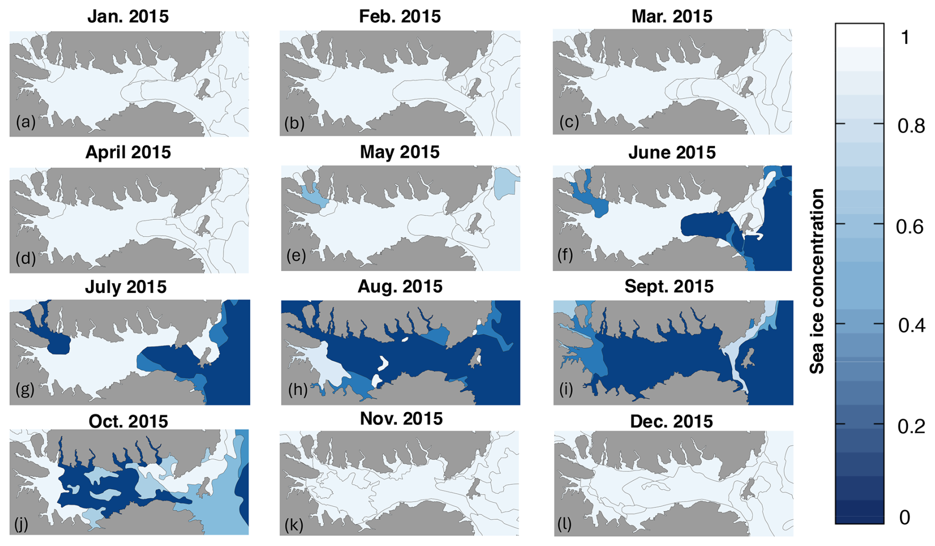
Figure 4 Monthly snapshots of sea ice concentration observations in 2015 from the Canadian Ice Service, which are created through the manual analysis of in situ, satellite, and aerial reconnaissance data (Canadian Ice Service, 2009). Gray shading denotes land.

We further evaluate the sea ice model by comparing monthly observed (Fig. 4) and modeled (Fig. 5) timestamps of 2015 sea ice concentration. While we only show the 2015 sea ice cycle, we note that the other yearly cycles feature similar spatiotemporal patterns of annual change. Observed 2015 sea ice concentration fields are taken from the Canadian Ice Service and are created through manual analysis of in situ, satellite, and aerial reconnaissance data (Canadian Ice Service, 2009). We find generally good agreement between the observed and modeled sea ice concentration states within Jones Sound for the 2015 sea ice cycle, with complete sea ice coverage simulated across the domain between November–April and nearly complete melt-back of sea ice in August and September. Importantly, we also find that our model is able to replicate the spatial pattern of sea ice melt-back, with flow through Fram Sound initiating sea ice decline in northwestern Jones Sound and partial clearing of sea ice across southeast Jones Sound. We note that modeled sea ice thickness east of Coburg Island is overestimated and sea ice does not clear out of this region during the summer months, disagreeing with observations. As such, in Sect. 3.4, we only integrate sea ice quantities west of Coburg Island.

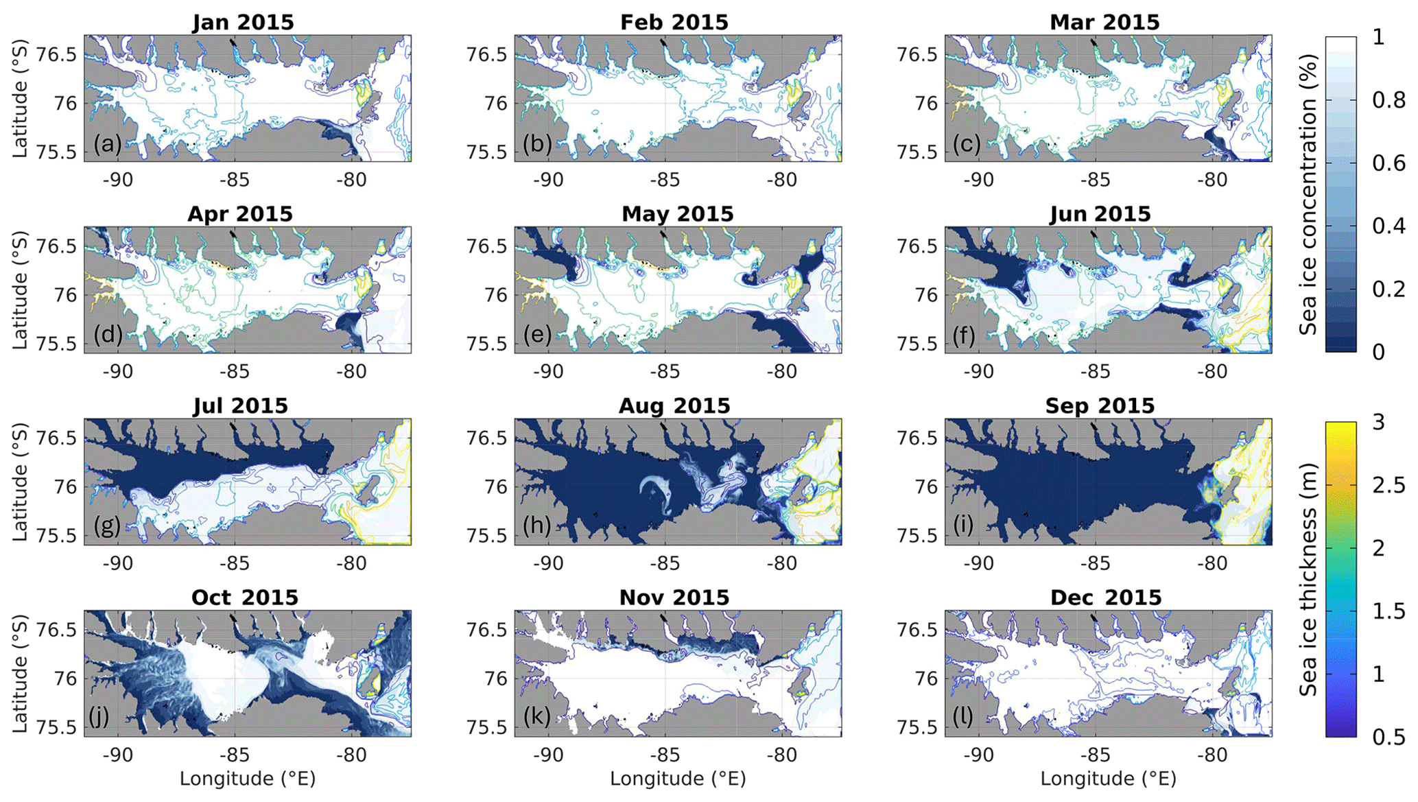
Figure 5 Monthly timestamps of simulated surface ocean grid cell sea ice concentration and contoured sea ice thickness (contoured every 0.5 m). Gray shading indicates land.

3.3 Ocean circulation through Jones Sound

Circulation through Jones Sound is dictated by flow through three waterways: Fram Sound (the confluence of Cardigan Strait and Hell Gates) in the northwest, Lady Ann Strait in the southeast, and Glacier Strait in the northeast. In Fig. 6a–d, we show time series (panels a–b) and time mean bar plots (panels c–d) of volumetric transport integrated through these three gateways into Jones Sound (lines in Fig. 8a). Of the temporal mean 1.31 Sv that flows into and out of Jones Sound, flow through Lady Ann Strait, Fram Sound, and Glacier Strait comprises 71.14 % (0.93 Sv), 14.26 % (0.19 Sv), and 14.40 % (0.19 Sv) of this volumetric transport, respectively (Fig. 6). Flow through each of these waterways is a mix of inflow and outflow into the sound; Lady Ann Strait is comprised of 0.37±0.12 Sv inflow and 0.56±0.15 Sv outflow, Fram Sound is comprised of 0.12±0.04 Sv inflow and 0.06±0.02 Sv outflow, and Glacier Strait is comprised of 0.16±0.09 Sv inflow and 0.03±0.03 Sv outflow (taken from Fig. 6c–d). Of particular importance is the influence of tidal flushing on transport through Fram Sound, enhancing its total volumetric transport by 47 %. For the other two waterways, tidal flushing had a minimal impact on total volumetric transport.

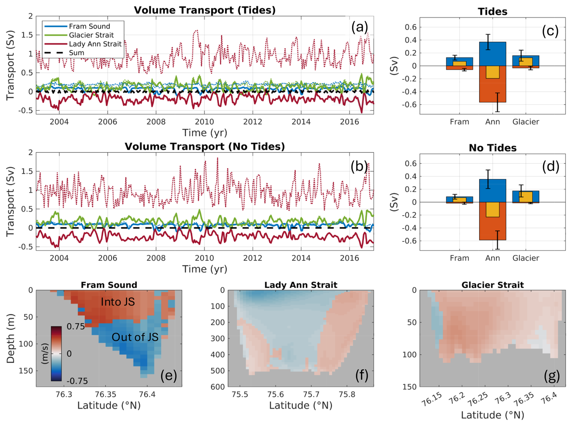
Figure 6 Time series of net transport (solid lines) and the magnitude (dotted lines) of volumetric transport through Fram Sound (blue), Glacier Strait (green), and Lady Ann Strait (red) with (a) tidal forcing included and (b) tidal forcing not included. Positive and negative values indicate transport into and out of Jones Sound, and note the different y-axis limits between the two panels. (c–d) Bar plots of the time mean transport into (blue) and out of (orange) Jones Sound, with the mean net transport indicated by the yellow bar. Panel (c) includes tides and (d) does not include tides. Error bars indicate 1 standard deviation from the mean. (e–f) Vertical cross sections of time mean ocean velocity through (e) Fram Sound, (f) Lady Ann Strait, and (g) Glacier Strait.

In Fig. 6e–g, we plot vertical cross sections of the 2003–2016 mean velocity fields through transects across Fram Sound (panel e), Lady Ann Strait (panel f), and Glacier Strait (panel g; yellow, red, and green lines in Fig. 8a, respectively) to visualize regions of flow into (red, positive) and out of (blue, negative) Jones Sound. Time mean ocean velocities through Fram Sound are the highest across all three waterways (maximum velocity of ∼ 0.7 m s⁻¹), with regions of inflow occupying the top 65 m of the water column and outflow located below (Fig. 6e). That is, while Fram Sound is the smallest waterway leading to Jones Sound by cross-sectional area, it has the second greatest integrated volumetric transport passing through it because of these high flow velocities. For Lady Ann Strait, the primary region of inflow is located near the south end of Coburg Island and persists through depth (Fig. 6f). We model a secondary weak region of inflow on the southern end of the strait below 200 m depth. Otherwise, outflow dominates circulation through the strait, with the strongest outflow velocities comprised of a persistent strong current that wraps around eastern Devon Island in the upper 100 m of the water column. Flow through Glacier Strait is dominated by inflow into Jones Sound, with a small region of outflow modeled on the extreme southern end of this waterway (Fig. 6g). Overall, these results highlight the complex spatial and temporal regimes of transport into and out of Jones Sound.

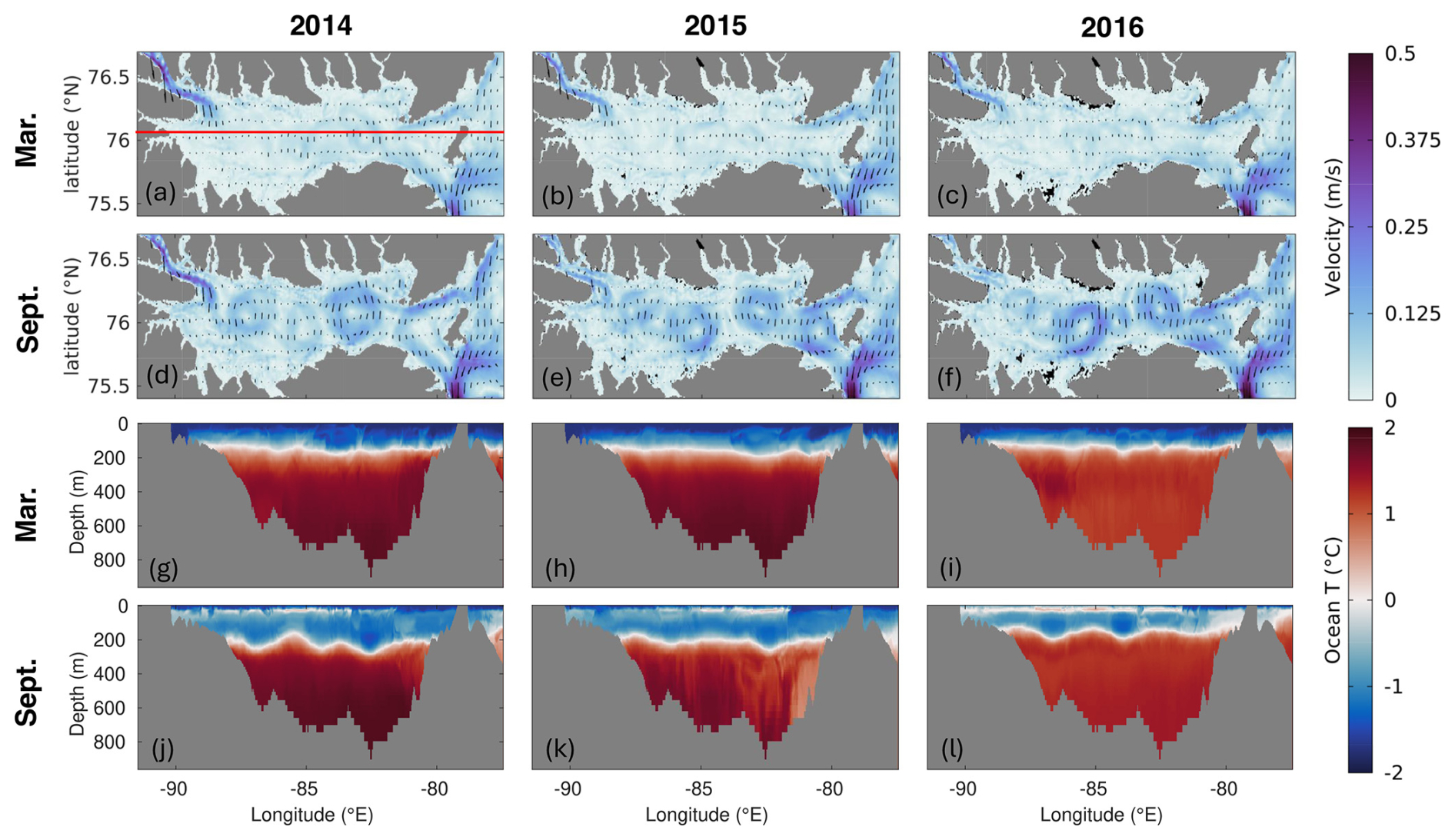
Figure 7 (a–f) Time and depth (down to 150 m) mean ocean velocity (m s⁻¹) fields with flow vectors overlaid. Panels (a)–(c) and (d)–(f) show March and September mean velocity fields, respectively. (g–l) Vertical profiles of ocean temperature (°C) taken along the red line in (a). Note that the first, second, and third columns show 2014, 2015, and 2016 mean fields, respectively.

In Fig. 7a–f, we show March (panels a–c) and September (panels d–f) mean ocean velocity fields that are averaged through 150 m depth for the years 2014 (panels a, d), 2015 (panels b, e), and 2016 (panels c, f). We selected March and September to capture circulation in which Jones Sound is completely covered with sea ice and completely sea-ice-free. In March under full sea ice coverage, the flow field is quiescent, with strong inflow (up to 0.5 m s⁻¹) through Fram Sound in the west and strong outflow (>0.5 m s⁻¹) through Lady Ann Strait in the east. The strongest currents from northern Baffin Bay tend to flow east of Coburg Island; however, we do simulate weak flow of up to 0.2 m s⁻¹ through Glacier Strait into Jones Sound. In September, however, reduced sea ice coverage allows atmosphere–ocean interactions, which drives the formation of persistent eddies that dominate circulation within Jones Sound (Fig. 7d–f). These eddies do not always form in the same place and rotate in the same direction. For instance, in 2014 (Fig. 7d), we model three sustained cyclonic eddies (rotating counterclockwise), where the easternmost eddy does not interact with strong inflow through Glacier Strait. In 2015 (Fig. 7e), we observe one anticyclonic eddy in the center of Jones Sound that is flanked by two cyclonic eddies, where circulation through Glacier Strait interacts with the easternmost eddy. Lastly, in 2016 (Fig. 7f), we model a similar eddy configuration as in 2015. The diversity of summertime circulation patterns across 2014–2016 in Jones Sound highlights the complex dependence of current patterns on inflow/outflow regimes and ocean–atmosphere interactions.

These circulation patterns influence the thermodynamic structure of the water column within Jones Sound. In Fig. 7g–l, we plot vertical temperature profiles across Jones Sound at 76° N (red line in Fig. 7a). As in the velocity fields, the third and fourth row of the figure correspond to March and September mean temperature fields, and the first, second, and third columns correspond to 2014, 2015, and 2016 fields, respectively. In all temperature fields, we note that the modeled thermal structure is homogeneous beneath the thermocline, as has been observed in Jones Sound (Fig. 3i). Under complete sea ice coverage, the modeled thermocline is nearly uniform at a depth of ∼ 100 m across Jones Sound (Fig. 7g–i). In September, the development of eddies drives spatial variation in the modeled depth of the thermocline, with the location of the eddy centers corresponding to locations of thermocline upwelling and downwelling. In September 2015, we see that the thermocline is nearly uniform at ∼ 200 m depth across Jones Sound, which is ∼ 100 m deeper than the March thermocline depth.

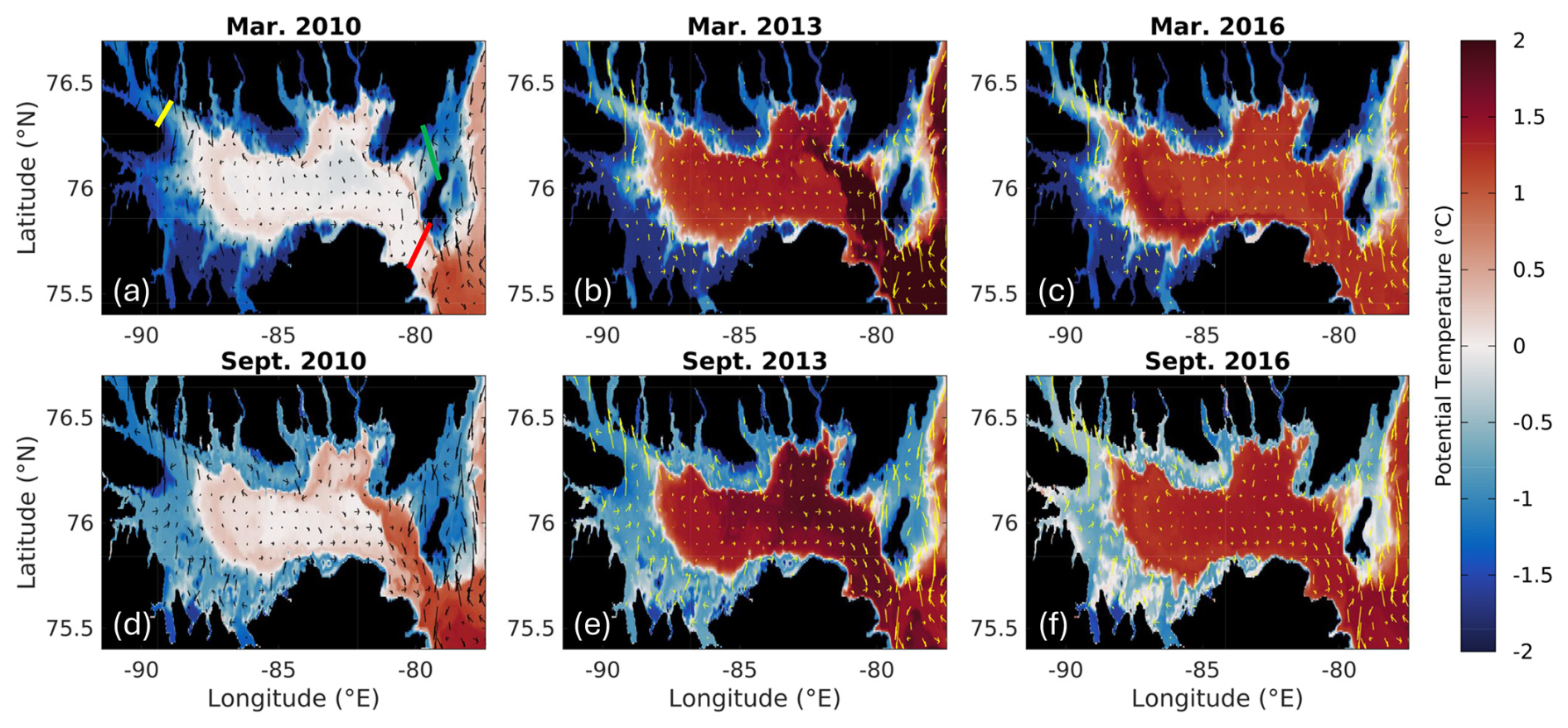
Figure 8 Modeled ocean bottom potential temperature (shaded) and velocity (vectors) in Jones Sound, Canadian Arctic Archipelago. The top row shows fields in March of (a) 2010, (b) 2013, and (c) 2016, while the bottom row shows fields in September (d) 2010, (e) 2013, and (f) 2016. In (a), the yellow, red, and green lines denote the location of the vertical cross sections through Fram Sound, Lady Ann Strait, and Glacier Strait that are shown in Fig. 6e–g, respectively.

The simulated spatial reach of warm waters below the thermocline in Jones Sound is topographically constrained. In Fig. 8, we plot the modeled ocean bottom temperature and velocity vectors in March and September of 2010, 2013, and 2016. As noted in the validation above, our model overestimates warming of waters below the thermocline in Jones Sound; however, as we correctly model the depth of the thermocline, we intend for the temperature fields shown here to be viewed as tracers of “warm” ocean water and its general circulation throughout the sound. It is evident that warm ocean waters flow into the model domain from the eastern model boundary, highlighting that the source of warm water inflow into Jones Sound is through northern Baffin Bay. This warm water then circulates into Jones Sound from the southeast through deep bathymetry that underlies Lady Ann Strait (> 600 m; Fig. 1). Inflow of deep warm ocean water is blocked by shallow bathymetry along Glacier Strait, which sits between 100–300 m depth. Once the warm bottom water intrudes into Jones Sound after 2010, it circulates counterclockwise, and although topographically constrained, warm bottom water breaches the entrance of most major fiords along the eastern periphery of the sound by 2012 (where bathymetry is generally deeper than that of the western sound). In particular, warm bottom water reaches the termini of Sverdrup, Jakeman, and Belcher Glaciers (Fig. A3). Depression of the thermocline in September relative to March constrains the reach of this warm bottom water. This can be seen in Brae Bay and western Jones Sound when comparing Fig. 8b and e. In regions where this warm water cannot circulate (regions of bathymetry above the thermocline), September water temperatures are ∼ 0.5 °C warmer than March water temperatures due to enhanced mixing.

3.4 Sea ice decline

Sea ice is a prominent feature of ocean circulation and dynamics within Jones Sound, regulating the exchange of heat, moisture, and momentum between the ocean and atmosphere, as well as blocking the penetration of sunlight that fuels photosynthetic biological productivity. In Fig. 5, we plot monthly timestamps of grid cell sea ice concentration and contoured sea ice thickness during model year 2015. Sea ice undergoes a yearly cycle in which the sound becomes largely ice-free in September and completely full of ice in the winter months. Oceanic flow through Fram Sound initiates sea ice decline in northwestern Jones Sound, typically beginning in April. Sea ice then retreats south across Jones Sound, clearing within the northern fiords first and then melting back across the rest of the sound by September. While most of the sound remains ice-free in September, Coburg Island acts as a sea ice bottleneck in our model (and in observations), trapping ice that circulates between the open waters of Baffin Bay and the confined waters of Jones Sound. During the winter, sea ice thickness generally fluctuates between 1–2 m across most of the sound. However, there are isolated pockets of thicknesses > 4 m, which are primarily constrained to within narrow fiords, along the periphery of Coburg Island, and in the open waters of Baffin Bay. This thick sea ice along Coburg Island and within Baffin Bay is not supported by observations and represents a model bias. We note that while we only show the 2015 sea ice cycle, these general patterns persist in other modeled years.

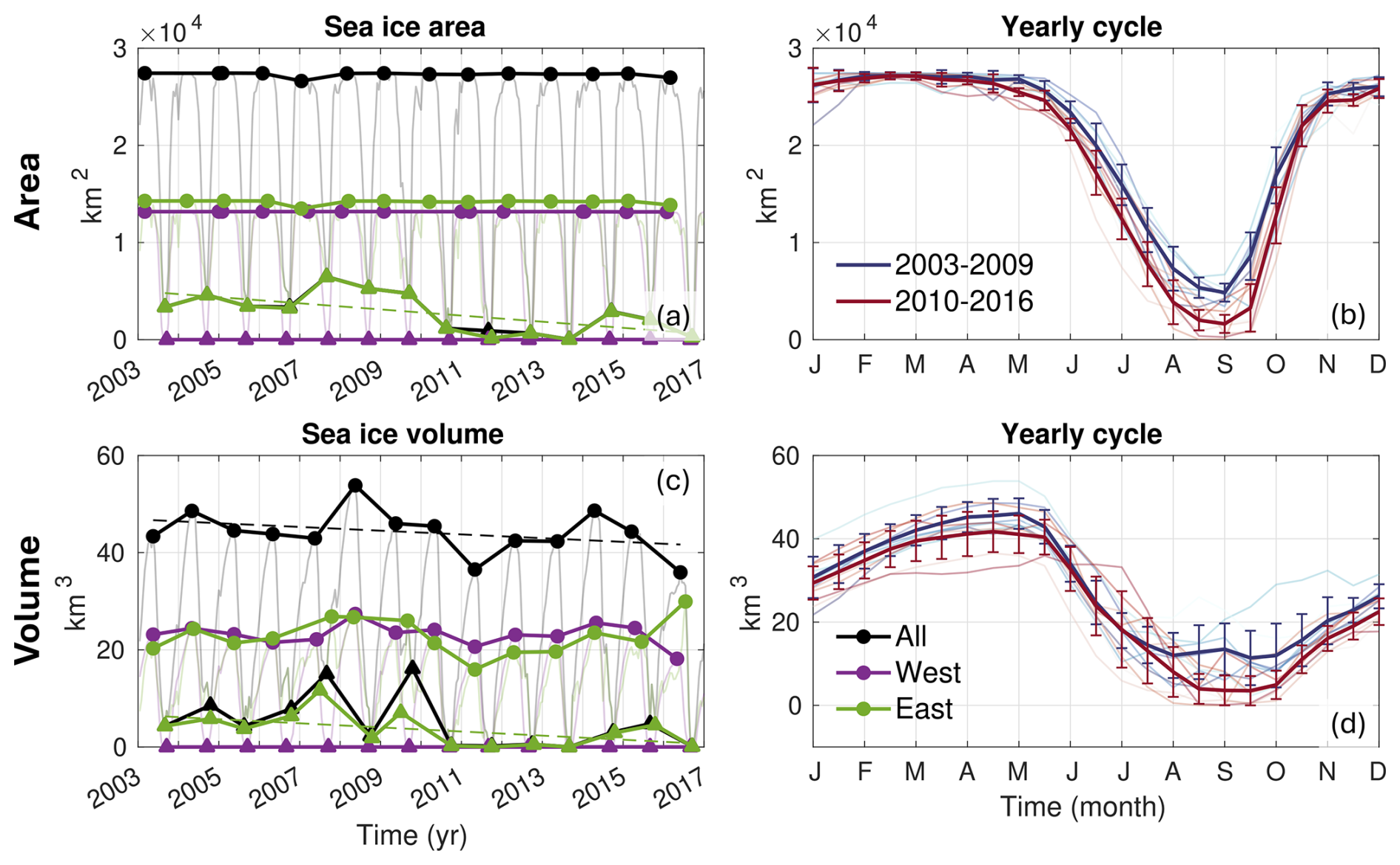
Figure 9 Integrated sea ice (a–b) area and (c–d) volume. In (a) and (c), marker colors correspond to the area of integration: black (all of Jones Sound), purple (western Jones Sound), and green (eastern Jones Sound). Circles and triangles denote yearly sea ice maxima and minima. Best-fit lines are overlaid on the eastern Jones Sound area and volume minima (green dashed lines) and the full Jones Sound volume maxima (black dashed line) to show long-term trends. In (b) and (d), the 2003–2009 and 2010–2016 mean yearly cycles and standard deviations are plotted as the blue and red lines, respectively. Each yearly cycle is overlaid as transparent blue or red lines.

To investigate how the annual sea ice cycle within Jones Sound changes between 2003–2016, we present integrated sea ice area (summed areas of grid cells that have a sea ice fraction greater than 0) and volume (area multiplied by the sea ice thickness) in Fig. 9 across the full extent of Jones Sound (using the western end of Coburg Island as our eastern limit; black lines), the western half of Jones Sound (purple lines), and the eastern half of Jones Sound (green lines). In Fig. 9, over these regions of integration, we plot the integrated sea ice maxima (circles) and minima (triangles) and overlay linear trend lines as dashed lines where trends are evident. In panels (b) and (d), we plot the average 2003–2009 and 2010–2016 yearly cycles of the aforementioned variables and their associated standard deviation, respectively. Beginning with the integrated sea ice area (Fig. 9a), we observe a temporal decline in minimum sea ice area of 316 km² yr⁻¹ in eastern Jones Sound, mainly associated with enhanced melt of sea ice pinned against Coburg Island and within eastern Jones Sound (Fig. 5). When the yearly total Jones Sound sea ice area cycles are binned to 2003–2009 and 2010–2016 and averaged (blue and red lines in Fig. 9b), we further observe that the initiation of sea ice decline occurs earlier and the onset of sea ice refreezing occurs later in the 2010–2016 profiles. Furthermore, although we find that winter sea ice area remains stable in our model (Jones Sound becomes completely ice-covered in winter), we observe that the thickness of this winter ice is declining with time (linear volume trend of −0.384 km³ yr⁻¹; black line with circles in Fig. 9c). In fact, the binned yearly cycles of sea ice volume reveal that sea ice is generally thinner throughout the entire yearly cycle aside from June and July (Fig. 9d).

To investigate the impact of tides on sea ice formation and melt within Jones Sound, we perform another simulation that does not include tides and find that tidal flushing through Fram Sound can enhance mean flow velocities by up to 0.75 m s⁻¹ over that of the non-tidal run in these regions (Fig. A6). These tidally enhanced flow velocities through Fram Sound trigger accelerated sea ice melt-back in northern Jones Sound between May and July (blue shading in Fig. A7e–g), while leading to generally thicker sea ice in the southwest sector of Jones Sound (due to ice advection into the southwestern fiords). Similar to Fig. 9, we integrate sea ice area and volume across Jones Sound and provide the associated time series in Fig. A8. Zooming into the 2014–2016 cycles, we find that tidal forcing drives a longer ice-free season within Jones Sound, decreasing the summer-integrated sea area by up to 6000 km² (Fig. A8b–c). Furthermore, tidal forcing also decreases sea ice thickness year-round due to both enhanced circulation velocities and mixing that entrains heat at depth to the surface (Fig. A8e–f).

3.5 Productivity enhancement

To begin deducing how these temporal changes in the state of Jones Sound sea ice and ocean circulation feed back on photosynthetic biological productivity, we couple our ocean–sea ice model to the MITgcm N-BLING biological productivity module and plot yearly integrated and depth-integrated profiles of net primary production (NPP; Fig. 10a), yearly integrated and depth-integrated profiles of chlorophyll mass (CHL; Fig. 10b), yearly integrated profiles of net community production (NCP; Fig. 10c, d), yearly integrated profiles of light limitation (Fig. 10e), and yearly integrated profiles of iron limitation (Fig. 10f). Light and iron limitation are computed as the percentage of ocean grid cells per vertical level that experience light or iron limitation, so a value of 100 indicates that 100 % of ocean grid cells are light- or iron-limited. NCP represents the difference between gross primary production and total community respiration; that is, when NCP is positive, photosynthetic primary productivity is greater than community respiration and vice versa when negative. In Fig. 10c and d, we observe that NCP increases in the first and second vertical ocean levels (corresponding to depths of 3.5 and 10.5 m, respectively, as the tracer point within MITgcm is in the mid-depth of the grid cell). When we zoom into the transition zone between positive and negative NCP, we further observe that the third ocean level (corresponding to a depth of 17.5 m) transitions from pure respiration before 2010 to a source of community production in the fall and summer beyond 2010. To investigate this further, we observe a strong increase in surface and subsurface NPP after 2010. Prior to 2010, total time-integrated surface (3.5 m depth level) NPP averaged ∼ 0.135 GtC yr⁻¹, and after 2010, it averaged ∼ 0.170 GtC yr⁻¹. These productivity enhancements are also elevated at 10.5 m depth (the second ocean depth level), where NPP before and after 2010 averaged 0.0051 and 0.0075 GtC yr⁻¹, respectively. We observe that the light limitation time series follows suit, as the mean percentage of summer light limitation of the surface level before and after 2010 is modeled as 48.08 % and 43.73 %, respectively. Similarly, at 10.5 m depth, the 2005–2010 and 2010–2015 mean summer light limitation is 64.24 % and 56.48 %, respectively. Interestingly, for the first two ocean depth levels (through 10.5 m depth), we observe that the percentage of ocean grid cells that are iron-limited in the summer increases after 2010; however, for these same levels, winter iron limitation steadily decreases throughout the simulation at a rate of ∼ 0.615 % per decade, implying more mixing. For depth levels below 10.5 m, the yearly cycle of iron limitation decreases linearly at approximately this same rate (yellow to red lines in Fig. 10f). We note that there are no temporal trends evident in the time series of phosphorus and nitrogen limitation and that both fields display decreasing percentages of limitation with depth.

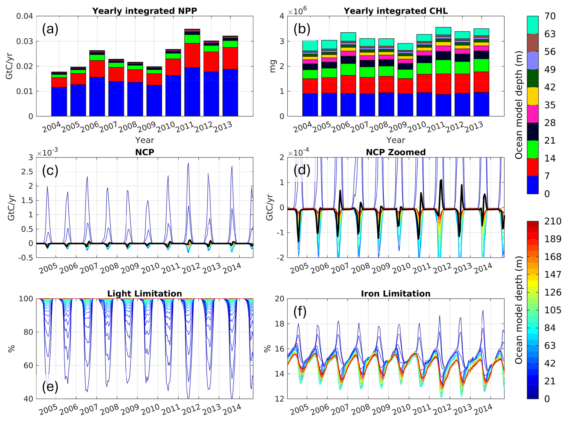
Figure 10 Bar plots of yearly and depth-binned (a) net primary productivity and (b) chlorophyll. Panels (c)–(d) show time series of net community productivity integrated on the top 20 vertical ocean levels (through 140 m depth), where the bold black line in (d) denotes values for the third vertical ocean level (17.5 m depth). Panels (e) and (f) show the percent of ocean grid cells per each vertical level that are light- and iron-limited, respectfully.

4 Discussion

4.1 Broader implications of Jones Sound circulation

The modeling results presented here highlight the dynamic ocean state and circulation patterns within Jones Sound as well as its joint impact on sea ice dynamics and biological productivity between 2003–2016. In our model, we find that the primary response of Jones Sound broad-scale atmospheric and oceanic changes is warming of the waters below 200 m depth. While the magnitude of this warming signal is overestimated in our model due to the Atlantic Water at our eastern model boundary warming too quickly in winter, we correctly model the depth of the thermocline as well as currents across our model domain, giving us confidence that we correctly simulate the spatial distribution of where these warmer mid-depth waters can circulate as well as volumetric transport throughout the domain. In particular, we find that circulation through Lady Ann Strait dominates volumetric transport into and out of Jones Sound, followed equally by Glacier Strait and Fram Sound. The magnitude of transport through Fram Sound reaches ∼ 0.25 Sv in summer months, agreeing with mooring data collected by Melling et al. (2008). These regions of inflow/outflow drive complex spatial patterns of circulation within Jones Sound, with the formation of multiple eddies driving variability in the thermocline depth in the summer. In the winter, under full sea ice coverage, the thermocline shoals under reduced atmospheric forcing. We further find that warm water within Jones Sound is topographically constrained, flowing through Lady Ann Strait and circulating counterclockwise within the sound, reaching many of the tidewater glaciers that line the sound's eastern coast (Figs. 8 and A3). In combination with continued observed atmospheric warming (Fig. 2a), these results underscore the increasing vulnerability of the ice masses that populate the Devon Island and Ellesmere Island.

Furthermore, our modeling results highlight the importance of circulation through Fram Sound in triggering sea ice decline in northern Jones Sound during the summer. Such relationships between tidal forcing and sea ice decline have been studied in other sectors of the Arctic and CAA (e.g., Rotermund et al., 2021; Armitage et al., 2020) but have yet to include Jones Sound due to the relatively small size of the channels that feed this waterway. The complex dependence of Jones Sound sea ice dynamics/thermodynamics on small-scale tidally forced ocean circulation features (as well as the importance of properly modeling sea ice change for summertime transportation through these waters) highlights the need for ocean models of this region to both explicitly include tidal forcing and be run at sufficient resolution to resolve the eddies that disperse subsurface heat.

In addition to these sub-annual patterns in simulated sea ice dynamics, we observe long-term declines in the Jones Sound integrated summer sea ice area as well as both the summer and winter sea ice volume. The summertime sea ice area declines on average ∼ 11 % per decade, which is in line with the observed losses over Baffin Bay of 11.7 % per decade between 1968–2022 and slightly higher than the 7.1 % per decade losses observed across all of northern Canada's waters over this same time period (Tivy et al., 2011). These losses mimic broader patterns of summer Arctic sea ice decline, which are cited to be driven by both natural climate variability (Kinnard et al., 2011; Ding et al., 2017, 2019) and human-induced global warming (Kay et al., 2011; Notz and Stroeve, 2016; Stroeve and Notz, 2018). Here, however, we show that winter sea ice in Jones Sound is also thinning (Fig. 9; winter sea ice area does not change over time but winter volume decreases with time), which is likely driven by winter warming of subsurface ocean temperatures (Figs. 2a and A5). Lastly, we simulate an earlier onset of sea ice decline in the summer and later onset of sea ice refreeze in the fall between 2003–2016. That is, the period of time in which Jones Sound is not completely filled with sea ice is extending in time in our model, which impacts the timing and integrated magnitude of photosynthetic oceanic primary productivity.

We observe in our biological modeling results that as the time during which Jones Sound is sea-ice-free becomes longer, the total integrated oceanic productivity and the depth at which productivity takes place increase. We note that aside from the atmospheric carbon dioxide forcing time series (which largely increases linearly), the boundary conditions in the biological productivity module do not include significant temporal trends and also do not account for nutrient release from enhanced glacial meltwater/discharge. That is, the response of ocean primary productivity in our model is driven primarily by changes in local oceanic and atmospheric conditions. Local enhancements to primary productivity have been reported across the Arctic, with the mean annual (March–September) trend of primary productivity increasing ∼ 50–75 g C m⁻² yr⁻¹ per decade within the central portion of Jones Sound between 2003–2022 (Frey et al., 2022). While this observed trend includes enhanced productivity due to increased nutrient availability from glacial runoff, the results presented here indicate that changing sea ice and ocean conditions are also partly responsible for driving these local enhancements to Jones Sound primary productivity. Plausible explanations that could either partially or wholly drive the simulated increase in Jones Sound productivity include (1) increased availability of light resulting from sea ice decline, (2) increased overturning of the mixed layer from enhanced wind stress as sea ice declines, resulting in greater nutrient upwelling, and (3) increased temperature of subsurface ocean waters possibly driving enhanced productivity since the carbon-specific photosynthesis rate in N-BLING is temperature-dependent (Galbraith et al., 2010; Noh et al., 2024). It is expected that a combination of these factors will drive enhanced productivity in our model, and this is evidenced in the light limitation and ocean temperature time series (Figs. 10e and A5, respectively). Specifically, we observe that the pattern of light limitation and ocean temperature through ∼ 31.5 m depth mirrors that of the yearly integrated chlorophyll mass. Beyond 2010, surface and subsurface light limitation and ocean temperature decrease and increase, respectively, driving enhanced productivity. In terms of nutrient limitation, we observe that iron limitation down to ∼ 10.5 m depth increases in the summer and decreases in the winter beyond 2010, possibly denoting increased vertical advection of nutrient-rich waters in the winter that drive productivity blooms once light becomes available. In all, these results highlight that the complex interplay between the atmosphere, ocean, and sea ice will likely continue to drive enhanced productivity in the future in Jones Sound under increasing polar-amplified global climate change.

4.2 Study limitations and uncertainties

The results presented here are subject to a high degree of uncertainty that stems from model limitations, the sparsity of input data used to drive and validate our model, and processes that are currently unaccounted for. As noted in the Methods section, N-BLING crashed in May 2015. Upon investigating the cause of this, it was determined that the pH of a coastal grid cell along the northern coast of Jones Sound reached infinity. In N-BLING, computing carbon chemistry requires carbonate alkalinity; however, we only model total alkalinity. As such, we must estimate carbonate alkalinity as the difference between total alkalinity and the contributions from borate, silicate, and phosphate. However, we do not model silicate and instead prescribe it. If simulated water properties in a grid cell become exceedingly fresh, the total alkalinity can become zero; however, silicate can never reach zero because we are prescribing it, causing the model to reach a threshold where total alkalinity is equal to silicate alkalinity (causing carbonate alkalinity to become zero). Thus, when N-BLING solves for pH, which has carbonate alkalinity in the denominator, it divides by zero, causing the model to crash. Future modeling studies can avoid this issue by directly modeling silicate or improving the N-BLING code to detect when silicate should be manually set to zero.

Furthermore, we previously noted that the ANHA12 ocean model output that was used to derive our ocean and sea ice model initial and boundary conditions features large warm biases in winter Atlantic Water (100–300 m), which then propagate throughout our model solution. We selected the ANHA12 model because it has sufficient resolution to resolve key circulation features in Baffin Bay and was also run through the time period of interest. However, this warm bias limits our model's ability to realistically simulate change in the thermal properties of mid-depth Atlantic Water, a key measure of the impact of global climate change on Arctic waters. In addition, errors in the bathymetry we use in our model, especially near coastal outlet glaciers, will lead to erroneous paths of warm water circulation. We corrected for bathymetry that was too deep near Sverdrup Glacier and too shallow near Grise Fiord; however, it is likely that there are other locations in Jones Sound in which the ocean bathymetry is incorrect and we do not yet have bathymetric observations to apply corrections. For the biological productivity model, recent studies have highlighted the importance of ocean–glacier interactions in driving near-glacier spatiotemporal patterns of productivity within Jones Sound. In particular, subglacial discharge plumes that originate beneath the nutricline can promote vertical advection of nutrients into the euphotic zone, while nutrient-rich glacial runoff can feed the upper ocean; both of these processes have been observed to drive coastal productivity blooms (Achterberg et al., 2018; Bhatia et al., 2021). While we do prescribe runoff as an atmospheric boundary condition in our ocean model, we assume it includes no nutrients and further do not resolve ocean–glacier interactions. As such, we do not capture the full extent to which atmospheric and oceanic warming drives change in Jones Sound productivity between 2003–2016, and we flag this as an important next step in this work.

In addition, Jones Sound remains understudied from both a modeling and observational perspective, which limits the amount of publicly available data that can be used as model inputs and validation. On the observational side, it is only since 2019 that recurring observational campaigns have targeted Jones Sound, so repeat oceanographic measurements only exist beyond this date. As such, ocean models of Jones Sound prior to 2019 must be validated based on how well they represent the time-evolving circulation within nearby Baffin Bay and Lancaster Sound, where annual repeat observations are available since the early 2000s. This is not sufficient, as the modeling results presented here demonstrate that while circulation within Jones Sound is driven by inflow from Baffin Bay and Fram Sound, water masses undergo transformation within Jones Sound and circulation around the sound is sensitive to small-scale bathymetric features. Furthermore, to our knowledge, this is the first publicly available ocean model that was developed and validated with the purpose of studying ocean circulation within Jones Sound, meaning that no other models of sufficient resolution exist to which we can compare modeling results. As Jones Sound is an important passageway of transport between the Arctic and Atlantic oceans and is critical in supporting local communities, we emphasize that future observational campaigns (especially within the inflow regions of Lady Ann Strait and Fram Sound) and modeling studies of Jones Sound should be prioritized so that we can gain a better understanding of the long-term impact of global climate change on this region and improve the fidelity of numerical ocean models.

5 Conclusions

In this study, we modeled ocean circulation, sea ice dynamics, and biological productivity within Jones Sound, Canadian Arctic Archipelago, between 2003–2016 with a high-resolution regional configuration of the Massachusetts Institute of Technology general circulation model. Atmospheric forcing was taken from the Arctic System Reanalysis version 2 and ocean boundary conditions were derived from a North Atlantic configuration of the NEMO ocean model (Hu et al., 2019; Gillard et al., 2020). We find that volumetric transport through the three waterways that connect Jones Sound to the Arctic and Atlantic oceans is partitioned as 71 %, 14 %, and 15 % via Lady Ann Strait, Fram Sound, and Glacier Strait, respectively. Surface circulation in the summer within Jones Sound is dominated by eddies, whereas winter circulation is quiescent due to sea ice cover. The spatial distribution of summertime eddies varies considerably year to year and drives variability in the depth of the thermocline across the sound, impacting the spatial reach of warm Atlantic Water that circulates at depth. This warm water, although topographically constrained, circulates counterclockwise around Jones Sound and expands its spatial reach in the winter when the thermocline shoals. Sea ice dynamics within Jones Sound are sensitive to small-scale circulation features that are generally not resolved within broad-scale CAA ocean models, such as tidal flushing through Fram Sound, which triggers sea ice melt-back in the spring. In addition, we find that wintertime sea ice thickness decreases and the onset of sea ice refreeze in the fall is delayed due to oceanic and atmospheric warming that is simulated in our model. These changes have the impact of lengthening the time during which and spatial extent to which Jones Sound is sea-ice-free, thus leading to enhanced productivity at all ocean depth levels through 17.5 m. While we note that the modeled warming signal in Baffin Bay and Jones Sound is overstated compared to observations, the results presented here improve our general understanding of circulation into, out of, and within Jones Sound as well as how it impacts sea ice and biological productivity dynamics. These results also emphasize the utility of high-resolution models in simulating complex waterways and underscore the need for sustained oceanographic observations in this region.

Appendix A: Additional figures

A1 Additional ocean model figures

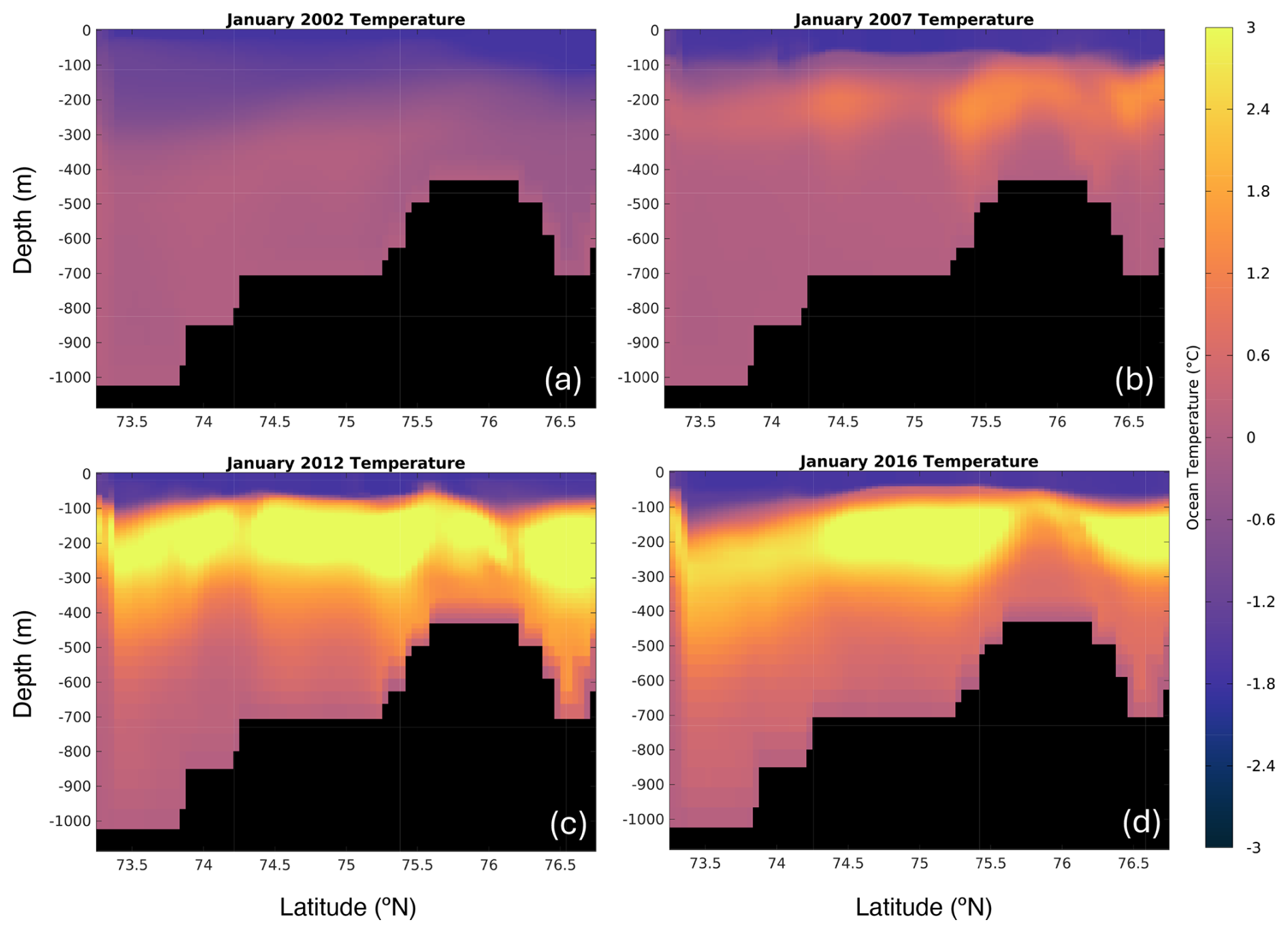
Figure A1 Vertical ocean temperature profiles (°C) of the eastern model boundary (in western Baffin Bay), taken from the ANHA12 NEMO ocean model in January of (a) 2002, (b) 2007, (c) 2012, and (d) 2016. Black shading denotes bedrock.

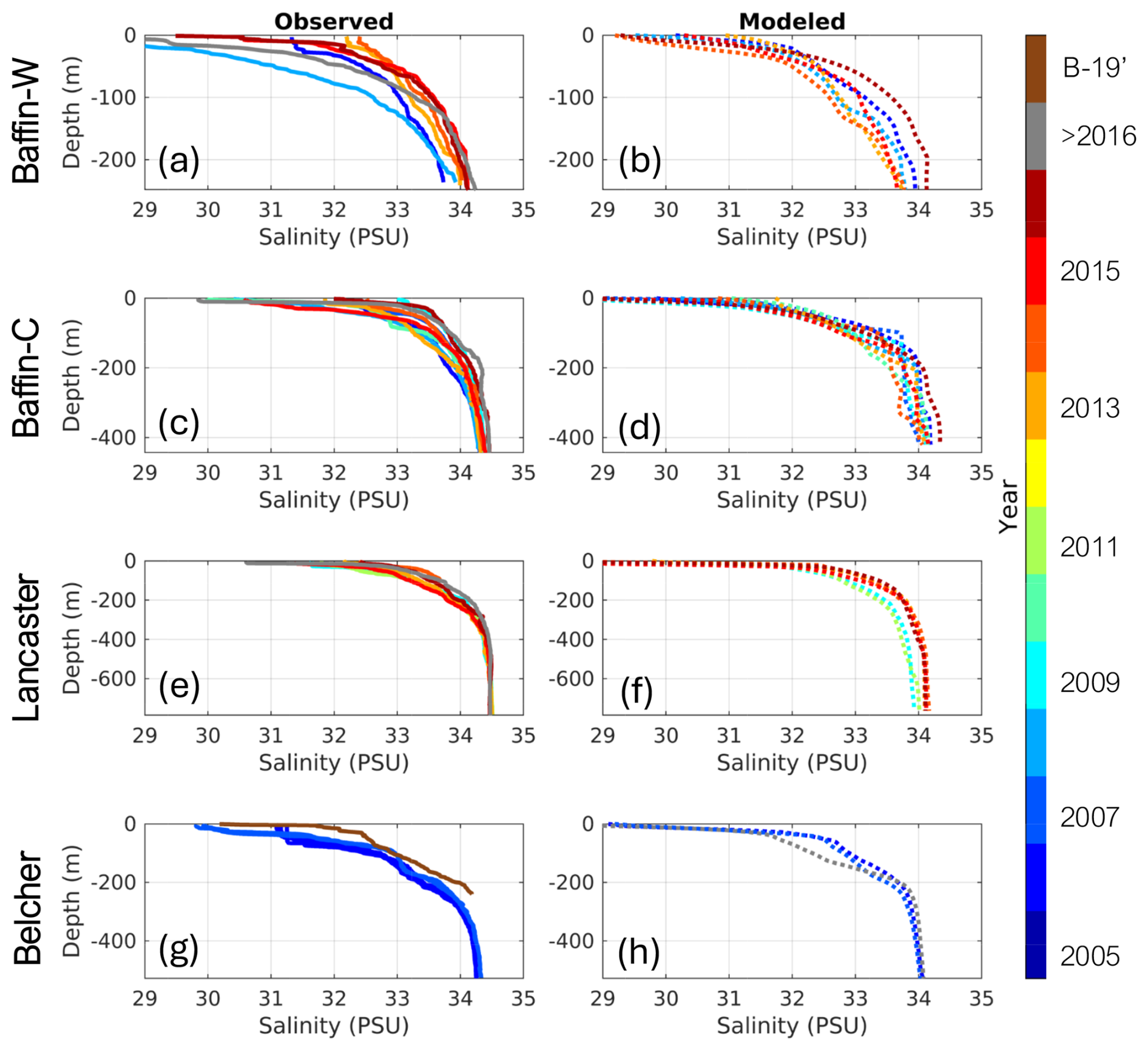
Figure A2 Same as in Fig. 3, but comparing modeled and observed vertical profiles of salinity (units on the practical salinity scale; PSU).

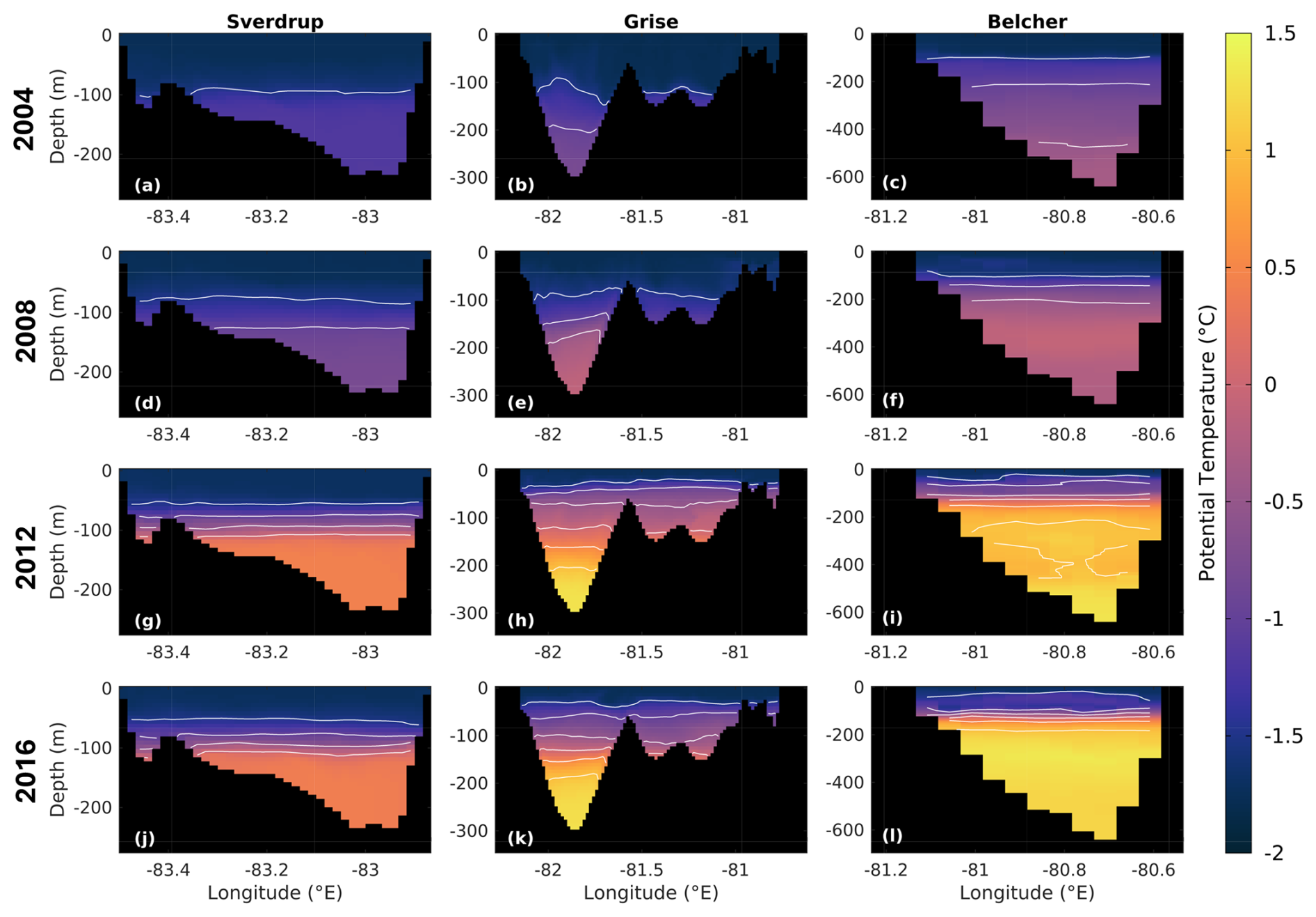
Figure A3 Vertical profiles of ocean potential temperature in April of (a–c) 2004, (d–f) 2008, (g–i) 2012, and (j–l) 2016 taken through (a, d, g, j) Sverdrup Bay, (b, e, h, k) Grise Fiord, and (c, f, i, l) the oceanic region adjacent to Belcher Glacier (white, yellow, and red lines in Fig. 8a). Areas of black denote land and white contours correspond to ocean temperature levels that start at −2 °C and increase in 0.5 °C increments.

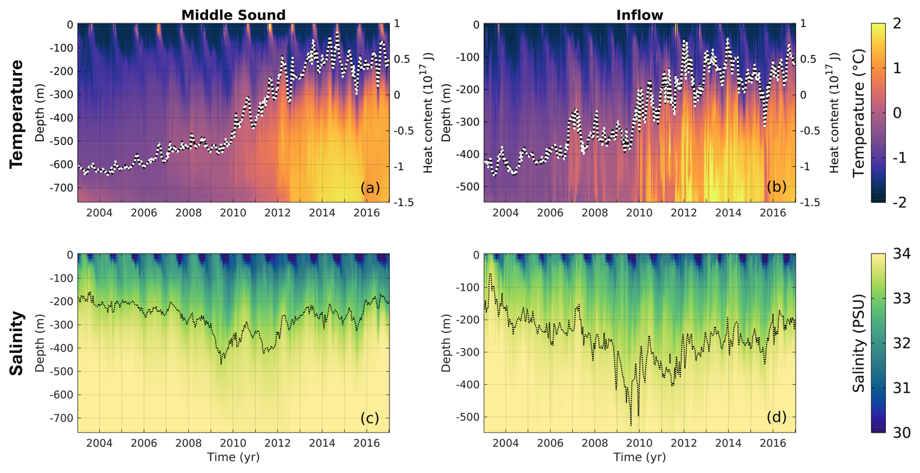
Figure A4 Depth–time Hovmöller diagram of (a–b) ocean temperature (°C) and (c–d) salinity (units on the practical salinity scale; PSU) taken at (a, c) the center of Jones Sound (green triangle in Fig. 8a) and (b, d) the center of Lady Ann Strait (orange circle in Fig. 8a). In (a) and (b), the white–black dashed line is the vertically integrated ocean heat content (10×10¹⁷ J) and corresponds to the right y axis. In (c) and (d), the black dotted line is the 33.80 PSU salinity contour.

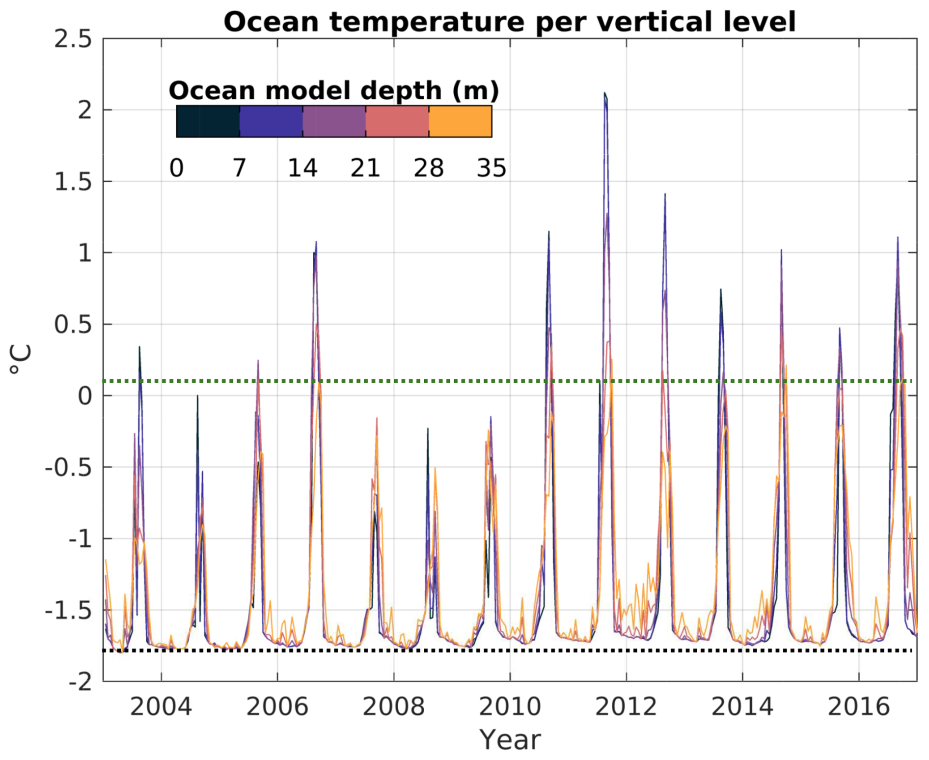
Figure A5 Ocean temperature time series (°C) of the first five ocean depth layers (0–35 m depth) taken in the center of Jones Sound. The black and green dotted lines mark the 2003–2010 mean maximum winter and summer ocean temperatures, respectively.

A2 Impact of tides on sea ice thickness

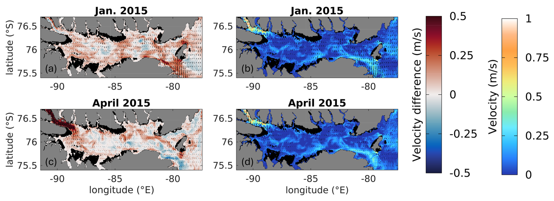
Figure A6 Magnitude (b, d) and difference (a, c) in 50 m ocean velocity in (a–b) January 2015 and (c–d) April 2015 between model runs with and without tides (red shading denotes where tidal forcing results in faster ocean velocities). Black shading denotes bathymetry above 50 m, and land is shaded in gray. Absolute velocities in (b) and (d) are taken from the model run with tides.

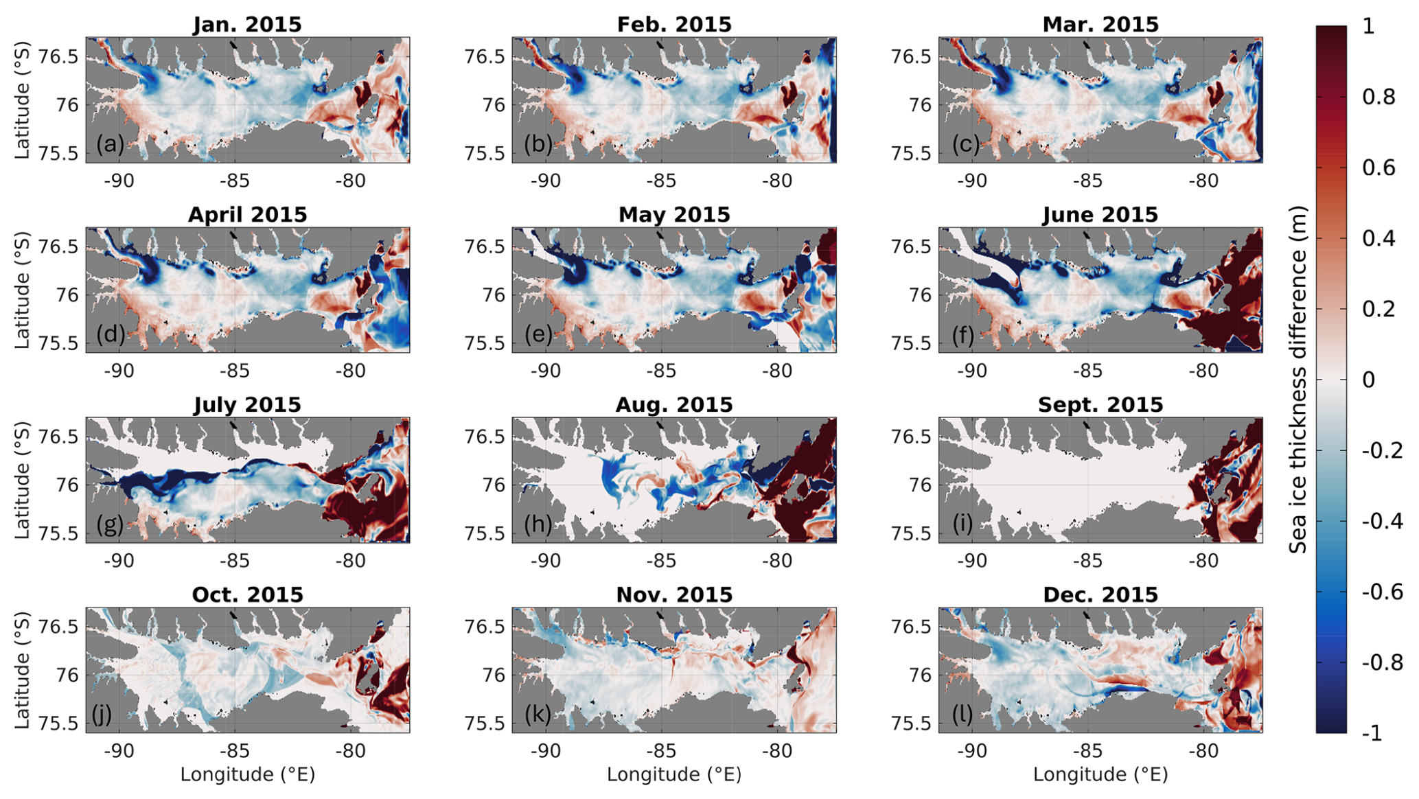
Figure A7 Difference in sea ice thickness between model runs with and without tides averaged each month of the year in 2015 (blue shading denotes where sea ice is thinner in the tidal run).

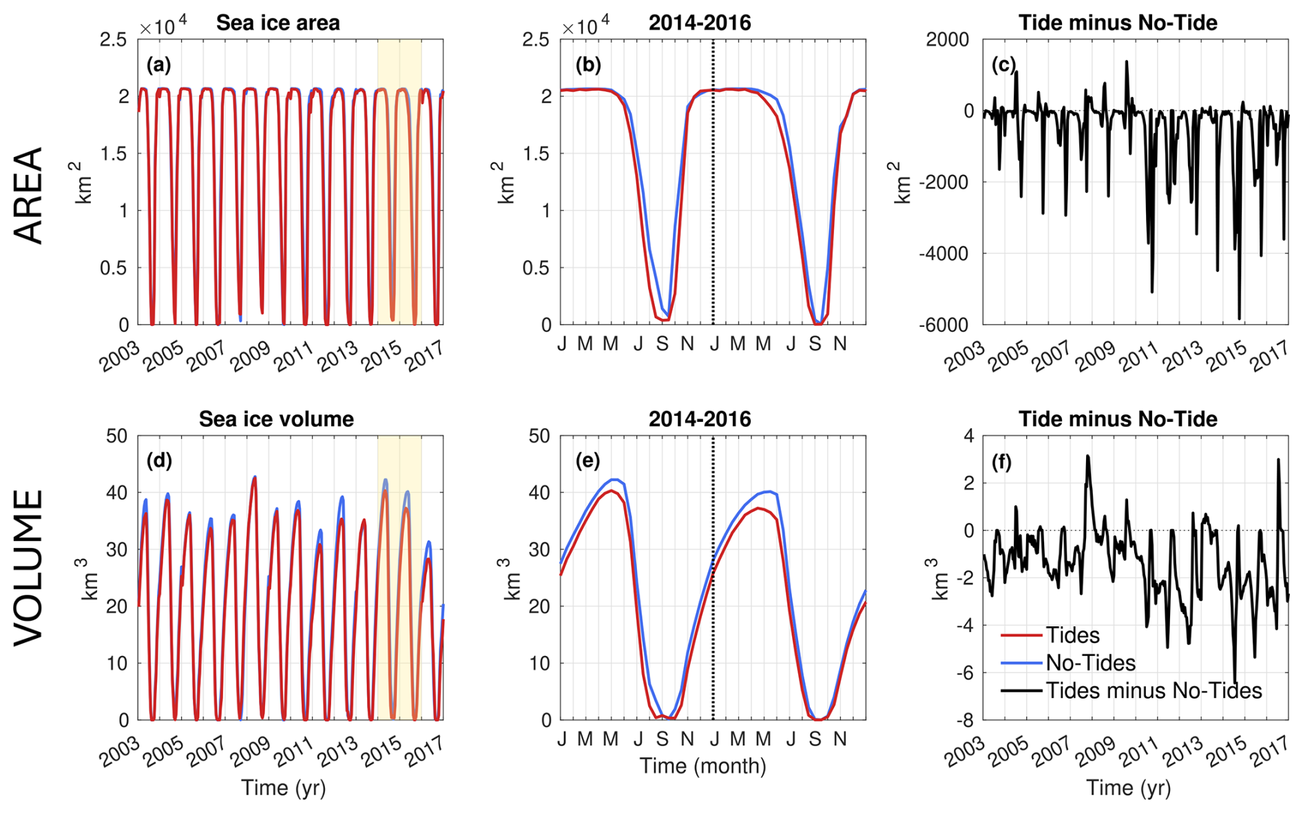
Figure A8 Jones Sound integrated sea ice area (a–c) and volume (d–f) time series, where red and blue lines represent results from the tidal and non-tidal simulation, respectively. Panels (b) and (e) are zoomed into the 2014–2016 sea ice cycle in (a) and (d), respectively. In (c) and (f), the black line denotes the difference of the tidal and non-tidal time series.