Marine heatwaves in the Mediterranean Sea: a convolutional neural network study for extreme event prediction

In recent decades, the Mediterranean Sea has experienced a notable rise in the occurrence and intensity of extreme warm temperature events, referred to as marine heatwaves (MHWs). Hence, the ability to forecast Mediterranean MHWs in the short term is an area of ongoing research. Here, we introduce a novel machine learning (ML) approach specifically tailored for short-term predictions of MHWs in the basin using an attention U-Net convolutional neural network. Trained on daily sea surface temperature anomalies (SSTAs) and gridded fields of MHW presence and absence between 1982–2017, our model generates a spatiotemporal forecast of MHW occurrence up to 7 d in advance. To ensure robust performance, we explore various configurations, including different forecast horizons and U-Net architectures, number of input days, features, and different subset splits of train–test datasets. Comparative analysis against a persistence benchmark reveals an improvement of 15 % in forecasting accuracy of MHW presence for a 7 d forecast horizon. We also demonstrate an improvement of MHW prediction accuracy as the forecast horizon decreases, albeit with a smaller discrepancy between the persistence benchmark, which also results in high accuracy for the 3 d forecasts. Our proposed ML methodology offers a data-driven prediction of MHWs with reduced computational requirements, which can be applied across different regions of the global ocean, providing relevant stakeholders and management authorities with essential lead time for implementing effective mitigation strategies.

1 Introduction

Since the 1980s, the Mediterranean Sea has experienced a mean sea surface temperature (SST) increase of approximately 0.041 °C yr⁻¹, which is twice the global average (Pisano et al., 2022). As a consequence, Mediterranean MHWs have increased in frequency, intensity, and spatial coverage, with profound disruptions of marine ecosystems and communities that rely on them (Smith et al., 2021); Specifically, MHWs have caused numerous mass mortalities of native and the migration of invasive species in the Mediterranean Sea (Garrabou et al., 2022), threatening the region's rich marine biodiversity and commercially valuable fish stocks (Lacoue-Labarthe et al., 2016). Consequently, the ability to forecast MHWs has become central to the field of extreme oceanic events in the basin as it enables the development of proactive measures for the mitigation of subsequent and potentially adverse effects on marine ecosystems and socio-economic activities.

Essential to the early prediction of MHWs are advanced monitoring systems and forecasting models, which have proven reliable for global (Schultz et al., 2021; Balaji, 2021) and regional applications (Konsta et al., 2023), in addition to sophisticated climate models that offer a comprehensive understanding of MHW drivers by simulating the complex interactions between atmospheric conditions and local oceanic circulation patterns (Darmaraki et al., 2019a). In the Mediterranean Sea, MHWs have been predicted in the short term by the regional Copernicus Mediterranean Forecasting System, which successfully captured phases of the summer 2022 event (McAdam et al., 2023), while climate models have projected MHW frequency and characteristics throughout the 21st century under different climate change scenarios (Darmaraki et al., 2019b; Konsta et al., 2023). However, forecasting systems and state-of-the-art numerical models present significant challenges due to the inherent uncertainties and chaotic nature of the climate system in addition to the associated high computational costs.

Thus, there is a growing interest in the use of machine learning (ML) techniques, particularly data-driven, deep learning models, to produce short- and long-term forecasts more efficiently (Schultz et al., 2021; Balaji, 2021). Deep learning models are used as surrogate models that overcome the computational constraints present in classical numerical weather prediction models. By training on large observational and/or model datasets, deep learning models can generate an extensive ensemble of forecasts, enhancing and complementing traditional numerical weather prediction models (Chattopadhyay et al., 2020). Compared to traditional methods, ML models typically encounter fewer issues with bias (Jacox et al., 2022) and are especially skilled at capturing and representing intricate and nonlinear dynamics in data (Hornik, 1991).

Current research predominantly focuses on the forecast of SST (Taylor and Feng, 2022), which allows for the establishment of contextualized thresholds based on specific requirements and conditions. This approach requires additional processing and expertise to identify MHWs (Hobday et al., 2016), which may complicate the application of these predictions by end users and management operators, a challenge that can be circumvented through data-driven spatiotemporal MHW prediction algorithms (Sun et al., 2023). Globally, the forecasting of SST using shallow ML techniques, such as linear regression and various statistical methods, is not new and dates back to the 1970s (Anding and Kauth, 1970; Fdez-Riverola et al., 2002; McMillin, 1975). During the last decade, the field has seen a significant shift towards the application of deep learning methods. These include recurrent neural networks, long short-term memory (LSTM) networks (Xiao et al., 2019; Liu et al., 2018), convolutional neural networks (CNNs) (Han et al., 2019), and hybrid methodologies that combine these techniques (Taylor and Feng, 2022). These advancements have enhanced the accuracy and capabilities of SST predictions.

In contrast, direct forecasting of MHWs has received less attention. For instance, Giamalaki et al. (2022) employed a random forest method and successfully forecasted spatiotemporal occurrences of MHWs in the North Pacific Ocean. However, their approach exhibited limitations in accurately predicting the intensity and duration of these events, underscoring the challenges in developing robust predictive models for such complex phenomena (Schultz et al., 2021). More recently, Sun et al. (2023) advanced the field by training a hybrid model that integrated CNNs with LSTM layers to predict the occurrence of MHWs. Their study proposed an innovative approach combining CNN-LSTM architectures with a U-Net CNN regression model to forecast both SST anomalies and binary classification maps, indicative of the presence or absence of MHWs in the future. These outputs served as indicators of MHWs when they exceeded certain thresholds. This hybrid method focused on predicting the spatial distribution of MHWs rather than generating simple time series forecasts and demonstrated significant potential for predicting MHWs with a lead time of up to 7 d. Such predictive capabilities can be particularly useful for the implementation of timely and effective mitigation strategies in regions highly vulnerable to MHW impacts, such as the Mediterranean Sea.

Nevertheless, the use of ML techniques for the early prediction of Mediterranean MHWs is an emerging field of research. One of the pioneering efforts has used artificial neural networks to predict the seasonal and inter-annual variability of SST in the western Mediterranean as well as the impact of the severe summer MHW of 2003 (Garcia-Gorriz and Garcia-Sanchez, 2007). By training on a variety of meteorological variables from 1960 to 2005, including 2 m air temperature, wind, and sea level pressure, the study achieved reliable monthly SST predictions. More recently, Bonino et al. (2024) evaluated the effectiveness of various ML algorithms, including LSTM networks, CNNs, and random forests on the forecast of daily SST, with a weekly lead time across 16 Mediterranean sub-basins. Their study focused on predicting SSTs that exceeded specific thresholds, indicating the potential occurrence of MHWs. This approach successfully reduced computational costs associated with the processing of 2D temperature fields, albeit at the expense of detailed information on the spatial variability of anomalous SST within each sub-basin. The results of this study outperformed outputs from the Copernicus Mediterranean Sea Analysis and Forecasting System, a sophisticated model that provides daily forecasts of ocean variables (Coppini et al., 2023). Overall, the application of ML techniques has showcased considerable potential in advancing our comprehension and forecasting of MHWs in the Mediterranean Sea.

Here, we combine well-established methodologies and tools to create a novel configuration of an attention U-Net CNN specifically tailored for the forecast of MHWs in the Mediterranean Sea. Using a minimal set of regional climate system model (RCSM) variables, primarily the daily spatial distribution of sea surface temperature anomalies (SSTAs) and spatiotemporal information on the presence and absence of MHWs in the basin produced by a MHW identification algorithm, we train the attention U-Net CNN model to forecast MHW occurrence 3 and 7 d in advance. This work is structured as follows: Sect. 2 describes the ML technique, the input variables that were used to train the U-Net model, and the error metrics used for validation. Results of MHW forecasting, based on various neural network configurations, are shown in Sect. 3 followed by the discussion and conclusions in Sect. 4.

2 Methodology

2.1 Study area

The Mediterranean is a semi-enclosed transitional area surrounded by the temperate zone to the north and the subtropical zone to the south and east. Its complex topography features sharp mountains, mild coastlines, and desert regions, creating a region highly sensitive to climate change. The Mediterranean Sea is connected to the Atlantic Ocean through the Strait of Gibraltar to the west and to the Black Sea via the Bosphorus Strait to the northeast, which serves as the main freshwater inflow for the eastern basin. It has a mean depth of 1500 m (Bethoux et al., 1999) and is divided in several sub-basins, including the Ionian, Tyrrhenian, Aegean, Adriatic, Alboran, Balearic, and Ligurian seas (Fig. 1). The region is also characterized by a distinctive thermohaline circulation driven by surface heat and water losses. This unique circulation system balances the excess evaporation over the Mediterranean, contributing to a net buoyancy flux towards the atmosphere, which plays a crucial role in the regional climate dynamics.

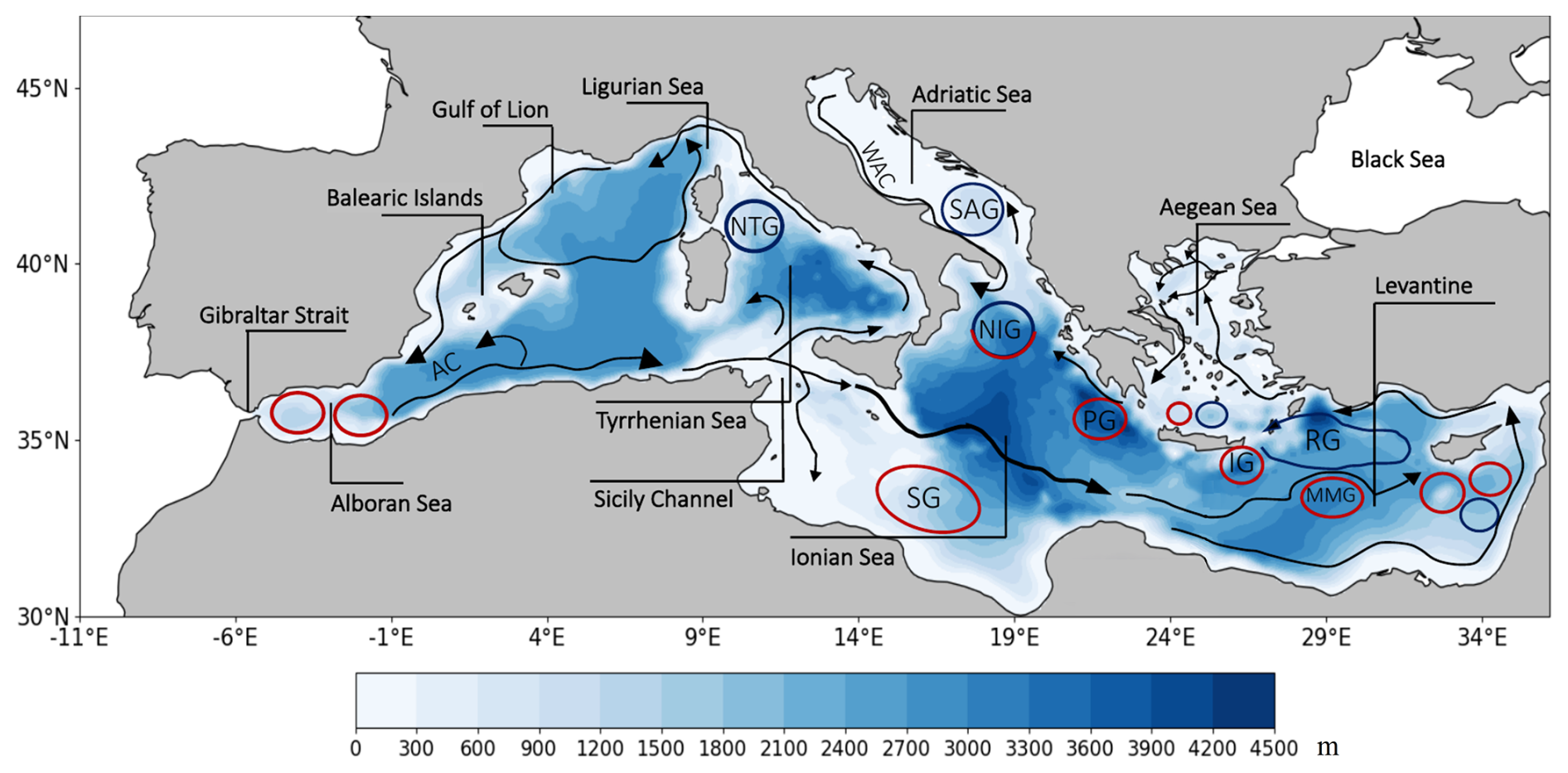
Figure 1 The bathymetry, main circulation, and sub-basins of the Mediterranean Sea. Key features of the surface circulation are shown with black arrows, with anticyclonic and cyclonic systems represented by red and blue circles, respectively. AC: Algerian Current‚ NTG: North Tyrrhenian Gyre‚ SG: Sidra Gyre‚ WAC: Western Adriatic Current‚ SAG: Southern Adriatic Gyre‚ NIG: Northern Ionian Gyre‚ PG: Pelops Gyre‚ IG: Ierapetra Gyre‚ RG: Rhodos Gyre‚ MMG: Mersa Matruh Gyre. Bathymetry (m) is given in colours based on the CNRM-RCSM6 model. The figure is reprocessed based on Menna et al. (2022), Velaoras et al. (2024), and Darmaraki et al. (2024).

2.2 Input data

To identify surface MHWs in the Mediterranean Sea and train the ML algorithm for their short-term prediction, we obtain daily gridded SST outputs from the fully coupled regional climate system model CNRM-RCSM6 that ran on hindcast mode between 1982 and 2017 (Sevault, 2024; Darmaraki et al., 2019a). The model (NEMOMED12) covers the entire Mediterranean Sea domain, has a 6–8 km horizontal resolution, with a varying vertical resolution, over 75 vertical levels in the ocean (Beuvier et al., 2012; Waldman et al., 2017), and its lateral boundary conditions come from ERA-Interim (Berrisford et al., 2009).

The ML method is trained, tested, and validated on a combination of two types of input variables: (1) daily gridded SSTA relative to the 1982–2017 period and (2) gridded fields of MHW presence/absence. The daily spatial coverage of surface MHW is computed using the updated version of the MHW detection algorithm by Hobday et al. (2016), available at https://github.com/coecms/xmhw (last access: May 2025) (Petrelli, 2022). According to this definition, a MHW occurs when the local SST is above a 30-year climatological period (1982–2014) and a threshold of the 90th percentile of SST for at least 5 consecutive days. The MHW identification method yields gridded binary classification masks of daily MHW presence/absence ($\mathrm{1}/\mathrm{0}$) for the entire Mediterranean Sea domain between 1982–2017. The predominant classification of grid points as MHW-absent (0) for most days of the year results in an imbalanced input dataset that affects the forecasting accuracy of any data-driven model (Bonino et al., 2024; Sun et al., 2023).

To achieve a more balanced input dataset and reduce memory requirements during training, the gridded MHW occurrence fields are first downsampled. This process considers a non-overlapping 2×2 submatrix around a point and assigns the label 1 in the presence of at least one MHW-affected pixel or the label 0 in its absence, leading to a decreased spatial resolution of MHW occurrence fields. The same approach is followed for points in the immediate proximity to the coast. The final spatial resolution of the Mediterranean Sea resolves to 128×72 points, which reduces the spatial resolution of the model to approximately 12–16 km. Despite the reduction in the spatial resolution, this approach increases the proportion of MHW presence to 14 % (from the initial 7.7 %) across the entire domain while still preserving a significant portion of the complicated Mediterranean Sea features and the geographical location of each MHW. To match the spatial resolution of the gridded MHW occurrence fields, we also downsample the daily SSTA of the Mediterranean Sea by means of spatially averaging within a non-overlapping 2×2 submatrix around a point. Daily SSTAs are further normalized to the range [0,1], aligning with the scale of the gridded MHW occurrence data, with a view to improve the prediction accuracy of the U-Net CNN (Xiao et al., 2019).

As an input to the CNN model for a given day, we insert the gridded fields of MHW occurrence and SSTA from preceding days, targeting the prediction of MHW spatial coverage 3 and 7 d ahead (Fig. 2). The limited set of input variables is selected as an effective approach to balance the risk of overfitting with computational efficiency in our method. This decision was further informed by a lagged correlation analysis, which revealed moderate correlations between SSTAs and atmospheric variables, such as air temperature, latent heat flux, and shortwave radiation, with SSTA displaying the highest-lagged autocorrelation (not shown). We then perform sensitivity tests to assess the impact of varying the number of preceding days as input, specifically 0, 2, and 4 d for the MHW occurrence fields and 5, 10, and 14 days for SSTA, on the model's predictive ability. Cosine and sine functions are also inserted as input features, indicating the yearly seasonal cycle, assuming a unique combination of values for each day of the year, spanning the period from 1 January 1982 to 31 December 2017:

$$\begin{array}{}\text{(1)}& \begin{array}{rl}{\cos }_t& =\cos \left({\displaystyle \frac{\mathrm{2}\mathit{\pi }t}{\mathrm{365}}}\right),\forall t\in \left\{\mathrm{1},\mathrm{2},\mathrm{\dots },N_{\mathrm{days}}\right\},\\ {\sin }_t& =\sin \left({\displaystyle \frac{\mathrm{2}\mathit{\pi }t}{\mathrm{365}}}\right),\forall t\in \left\{\mathrm{1},\mathrm{2},\mathrm{\dots },N_{\mathrm{days}}\right\},\end{array}\end{array}$$

where the total number of days is denoted by N_days.

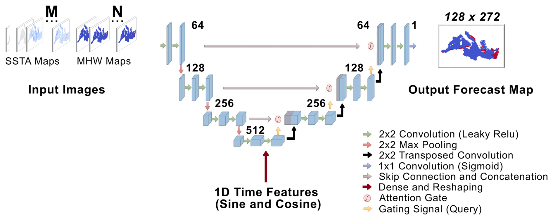
Figure 2 Attention U-Net CNN model architecture to forecast MHW presence/absence maps. N and M are the number of input frames containing spatiotemporal information on MHW presence/absence and SST anomaly, respectively. Each map corresponds to daily frequency of input data and has a matrix size of 128×272. The U-Net figure is adapted from Ibtehaz and Rahman (2020).

2.3 The attention U-Net CNN model

In this study, we employ a data-driven approach, which means that the nature, quantity, and quality of our data (e.g. number of available years; temporal discontinuities in data; spatiotemporal resolution and forecasted variable characteristics, including class imbalance, seasonality, and randomness) dictate the methodological choices for forecasting MHW occurrence across different time horizons. Using a neural network architecture, enhanced with attention mechanisms (attention U-Net CNN mode) which emphasize key features while suppressing noise and capturing important spatiotemporal patterns, we focus on 3 and 7 d forecast horizons. This is deemed a sufficient time for proactive decision-making by authorities and local stakeholders before a MHW incident (Giamalaki et al., 2022).

2.3.1 Attention U-Net architecture

Here, the prediction of MHWs is considered a supervised classification/regression challenge, for which we employ the specific neural network architecture illustrated in Fig. 2, based on the U-Net CNN architecture proposed by Ronneberger et al. (2015). Due to the use of several intermediate (hidden) layers, the method is classified as a deep neural network category, with the architecture including both a contracting and expanding path. The contracting path is responsible for extracting features from the input data and progressively reducing the size of the feature maps through downsampling, which, in our case, consists of a series of three max pooling layers (https://www.tensorflow.org/api_docs/python/tf/keras/layers/MaxPooling2D, last access: March 2024). This process effectively increases the model's ability to perceive broader spatial relationships. As the contracting path progresses, the number of channels in the feature maps is doubled to improve feature capture across different scales. Conversely, the expanding path uses upsampling operations to restore the feature maps to their original dimensions, consisting of three deconvolution layers, using a Conv2DTranspose (https://www.tensorflow.org/api_docs/python/tf/keras/layers/Conv2DTranspose, last access: March 2024) for the decoding path, as shown in Fig. 2.

Moreover, the model incorporates skip connections to integrate both local and global features, enabling the network to utilize information from various scales simultaneously. Attention gates are placed before concatenating the skip connections, automatically learning to focus on target structures of varying shapes and sizes. This design is expected to improve the model's prediction accuracy while maintaining minimal computational overhead (Oktay et al., 2018). The architecture also includes 2D convolutional layers with 2×2 kernels between all layers. The number of neurons in each layer follows an exponential pattern with a base of 2, increasing in the contracting path and decreasing in the expanding path. The sine/cosine time features from Eq. (1) are incorporated at the bottom of the encoding path after passing through dense and reshaping layers to obtain the same spatial dimension as the layer with which are concatenated.

Due to its versatility, this method has been previously used in studies of image segmentation, pattern identification (Oktay et al., 2018; Srivastava et al., 2014), spatiotemporal forecasting (Jacques-Dumas et al., 2022), and downscaling at higher resolutions with minimal computational cost (Doury et al., 2023) and has been shown to significantly enhance the accuracy of forecasts. The goal of this network is to determine the probability of each grid point being classified as either MHW-present (1) or MHW-absent (0) for predictions of 3 or 7 d ahead, thus forecasting the spatiotemporal probability of MHW occurrence.

2.3.2 U-Net CNN model training

A common practice in a neural network approach is the splitting of a dataset into the training, testing, and validation subsets. Here, the validation dataset consists of the early years from 1982 to mid-1986, the training dataset comprises the years from mid-1986 to mid-2013, and the final years selected for testing and validation of the model span mid-2013 to 2017. Following the split, each of the three subsets (train, test, and validation) undergoes random internal shuffling to reduce memorization effects and increase the robustness of the forecasting tool. The tendency for a model to memorize rather than learn meaningful patterns – known as overfitting – is a critical challenge in neural network training as it leads to excessive tuning to the training data and causes the model to capture noise and irrelevant details, ultimately compromising its ability to generalize effectively to new, unseen data. To further reduce overfitting effects, we employ a “dropout” approach, which involves random deactivation of a specified number of nodes, set to 30 % here, during each training step (Srivastava et al., 2014). An early-stopping/best-saving checkpoint mechanism is also implemented whereby the training process halts if there is no improvement for a predetermined number of epochs and a selected validation metric (i.e. mean squared error, accuracy, recall, and F₁ score).

Throughout the training of our model, we employ the Adaptive Moment Estimation (Adam) optimizer (Kingma and Ba, 2014), an optimization algorithm, which is based on two gradient descent methodologies, with a batch size of 4 and an initial learning rate of 0.001, set up to reduce by half on a plateau of 10 epochs, with a minimum learning rate of 10⁻⁴ and maximum number of 100 epochs. Evaluated across all the training samples, the Adam optimizer is used here to minimize the loss function, a key parameter of the attention U-Net CNN, which measures the discrepancy between predicted and actual values. The model's ability to successfully perform a given task is determined by the choice of the loss function and the effective reduction of prediction errors. Given the binary form of the MHW presence (1) and absence (0) fields, the use of a binary cross-entropy loss function is a common choice (Jacques-Dumas et al., 2022). In the case of extreme events and imbalanced datasets, where one of the two classes is underrepresented, the focal binary cross-entropy is preferred (https://www.tensorflow.org/api_docs/python/tf/keras/losses/BinaryFocalCrossentropy, last access: March 2024) (Lin et al., 2020). This function further improves the effects of the standard binary cross-entropy by integrating two additional parameters designed to reduce the influence of correctly classified samples and emphasize the importance of misclassified ones. We use this loss function, which in equation form reads as

$$\begin{array}{}\text{(2)}& \begin{array}{rl}\mathrm{Focal}\left(p_t\right)& =-\sum ^{N\cdot M}{\mathit{\alpha }}_t{\left(\mathrm{1}-p_t\right)}^{\mathit{\gamma }}\log \left(p_t\right),\\ & \text{where}{p}_t=\left\{\begin{array}{ll}p,& y=\mathrm{1}\\ \mathrm{1}-p,& \text{otherwise}\end{array},\right.\end{array}\end{array}$$

where y is the ground-truth class, $p\in [\mathrm{0},\mathrm{1}]$ is the predicted probability, and α_t and γ are the tuning parameters, which are selected to be 0.25 and 2, respectively, following Nguyen and Thai (2023). This adjustment leads to elevated loss values when misclassifications occur, steering the training process toward lower local minima of the loss function. Due to the nonlinear nature of the patterns the neural network is trained on and despite the attempts to minimize the loss function, its convergence often leads to near-local minima, impeding its performance. To improve the model's performance and ensure that minima values of the loss function maintain satisfactory accuracy levels in their prediction, several iterations with varying parametric choices are conducted on test cases (see Results Sect. 3.2, Table 1).

An additional aspect of neural network architecture is the selection of activation functions, which are applied to the outputs of each intermediate hidden layer. These functions have a key role in determining the operations applied to the input neurons and thereby the model's ability to generate an output (Sharma et al., 2020). In this study, we overcome the limitations associated with the use of a standard rectified linear unit (ReLU) activation function in handling negative input values using a leaky ReLU version in all the intermediate layers (Maas et al., 2013). The leaky ReLU function allows a small, non-zero gradient for negative inputs, effectively mitigating the vanishing ReLU problem, where neurons become inactive during training. This effect proves advantageous for nonlinear prediction tasks, enabling the model to capture a broader range of input variations. The output (final) layer is equipped with a sigmoid activation function, which is appropriate for binary classification tasks as it produces values within the range of [0,1]. These values express the probability for a grid point being affected by a MHW, with the classification threshold determined by the specific characteristics of the physical problem in each instance. The process by which we select the appropriate classification threshold is further discussed in Sect. 3.1.

The U-Net CNN model described here was implemented using the Keras API and using TensorFlow 2.9.2 in Python. The architecture outlined in Fig. 2 required 32 million parameters to train, and it ran in parallel on eight NVIDIA A100 GPUs with a memory of 40 GB each in one node of the p4d.24xlarge Amazon EC2 server. Each test case required approximately 4 h to complete the training of 100 epochs, and the inference speed required seconds to calculate forecasts for each sample on the same server. We note that once the computationally expensive training ends, the model can be deployed to any system to generate forecasts, with minimal computational overhead, given the appropriate input data. For instance, the inference time for the entire testing dataset, consisting of 1300 daily forecasts, required approximately 60 s on the aforementioned hardware configuration.

2.4 Evaluation metrics

The model's performance is evaluated on a testing dataset consisting of samples that were obscured by the U-Net CNN during its training phase. At this stage, we assess the model's ability to accurately predict unseen data and determine the optimal probability threshold above which each grid point is categorized as a MHW-affected case. Throughout the training and validation process, standard metrics such as recall, accuracy, and selected loss function are calculated during each epoch for the training dataset and at the end of each epoch for the validation dataset (https://www.tensorflow.org/api_docs/python/tf/keras/metrics, last access: March 2024). The primary metric to evaluate the prediction skill of the attention U-Net CNN regarding future MHW occurrences is the true positive rate (TPR). This rate assesses the proportion of accurately predicted MHW occurrences relative to the total number of actual occurrences (Sun et al., 2023). The formula for calculating TPR is given by

$$\begin{array}{}\text{(3)}& \mathrm{TPR}={\displaystyle \frac{\mathrm{TP}}{\mathrm{TP}+\mathrm{FN}}},\end{array}$$

where TP represents true positive predictions and FN denotes false negative ones. In other words, the TPR metric quantifies the model's ability to accurately detect true MHW occurrences during testing. At the end of each epoch during the training process, validation recall, a metric similar to TPR, is computed on the validation subset and serves as an early-stopping mechanism, a technique useful for both computational efficiency and preventing overfitting. In contrast, the true negative rate (TNR) evaluates the model's ability to accurately predict the negative class labels, specifically the absence of a MHW, relative to the total number of non-MHW occurrences. This metric is defined as

$$\begin{array}{}\text{(4)}& \mathrm{TNR}={\displaystyle \frac{\mathrm{TN}}{\mathrm{TN}+\mathrm{FP}}},\end{array}$$

where TN represents the true negatives and FP the false positives. Combining these two rates, the forecast accuracy rate (FAR) composite metric can be used to assess the model's overall forecasting ability. Unlike the TPR and TNR, which focus on a single class, the FAR considers both the correct and incorrect MHW predictions across all classes. In formula form, FAR is defined as

$$\begin{array}{}\text{(5)}& \mathrm{FAR}={\displaystyle \frac{\mathrm{TN}+\mathrm{TP}}{\mathrm{TN}+\mathrm{FP}+\mathrm{TP}+\mathrm{FN}}},\end{array}$$

providing a percentage-wise estimation of forecast accuracy.

To obtain an overall TPR, TNR, and FAR as single numerical indicators for each sample in the testing dataset, we separately average the metrics defined in Eqs. (3), (4), and (5) over the Mediterranean Sea domain. This approach provides a single spatially independent numerical value for each error metric corresponding to each sample in the testing dataset. The final TPR, TNR, and FAR for each forecast horizon are determined by averaging each of these metrics across all test samples.

2.5 Persistence benchmark

A standard approach to evaluating the predictive skill of our ML model is to compare its output forecast with a climatological baseline derived from a persistence benchmark model, which assumes that MHW presence or absence, within the next 3 or 7 d, remains constant throughout the forecast period. Specifically, the persistence benchmark uses MHW presence/absence fields from 3 or 7 d prior to an event as both the input and the forecast for the target MHW conditions. By operating under the assumption that recent MHW conditions persist into the forecast period, the persistence model provides a baseline performance level against which we assess whether the U-Net CNN model adds predictive value beyond simple temporal persistence. Despite the simplicity of this assumption, using the persistence benchmark model as a reference dataset is a meaningful approach for short-term forecasting (Parasyris et al., 2022) given the relatively slow changes in SST, which lead to minimal variations in MHW presence on most consecutive days. Improvements demonstrated by the output forecast of a neural network model that surpasses the basic persistence model are essential for accurately forecasting the onset and dissipation of MHWs.

3 Results

3.1 Assessing the probability of MHW occurrence

The output probabilities of MHW occurrence are converted into binary classification masks as an initial step to assess the forecast ability of our ML model. In particular, the U-Net CNN generates maps where each pixel value ranges between 0 and 1, representing the probability of each grid point being a negative (MHW-absent) or positive (MHW-present) class (referred to as forecast probability). A range of forecast probability thresholds (hereafter threshold) is then evaluated from 0.05 to 0.9, in increments of 0.05, as a trial-and-error technique, to find the one which maximizes a specific accuracy metric (TPR, TNR, FAR). A prediction based on each threshold is subsequently generated for the entire testing dataset and compared with the true MHW occurrences originally identified using the climate model output. Following the work of Sun et al. (2023), we first compute the spatially averaged TPR and TNR separately for each threshold and further average their sum for all samples within the test set. The optimal thresholds for the 3 d (Fig. 3a) and 7 d (Fig. 3b) forecast scenarios are then determined by maximizing this combined mean (CM) of TPR and TNR, which is formulated as

$$\begin{array}{}\text{(6)}& \mathrm{CM}={\displaystyle \frac{\mathrm{TPR}+\mathrm{TNR}}{\mathrm{2}}}.\end{array}$$

In both scenarios, increasing the threshold results in a higher TNR and lower TPR as more predictions are classified as MHWs absences, the accuracy of which is thereby improved. The intersection point in each forecast scenario (Fig. 3, red star) represents an equilibrium between sensitivity and specificity in classification terms. This point maximizes the CM (Fig. 3, green lines), optimizing predictive performance of both the positive and negative MHW occurrences. Specifically, the optimal threshold for the 3 d forecast is identified at 0.45, yielding a maximum CM of 0.89 (Fig. 3a), whereas the 7 d forecast achieves a CM of 0.77 at an optimal threshold of 0.4 (Fig. 3b). At a high threshold of 0.85, both scenarios exhibit a TNR close to 1, indicating no false negatives, as most predictions are classified as negative. However, at this threshold, the respective TPR is 0.48 for the 3 d forecast and 0 for the 7 d forecast (Fig. 3, blue lines). This suggests that for the 3 d forecast, half of the MHWs were correctly classified despite the excessively high threshold. In contrast, the 7 d forecast shows a decline in performance as TPR is approximately zero (Fig. 3b).

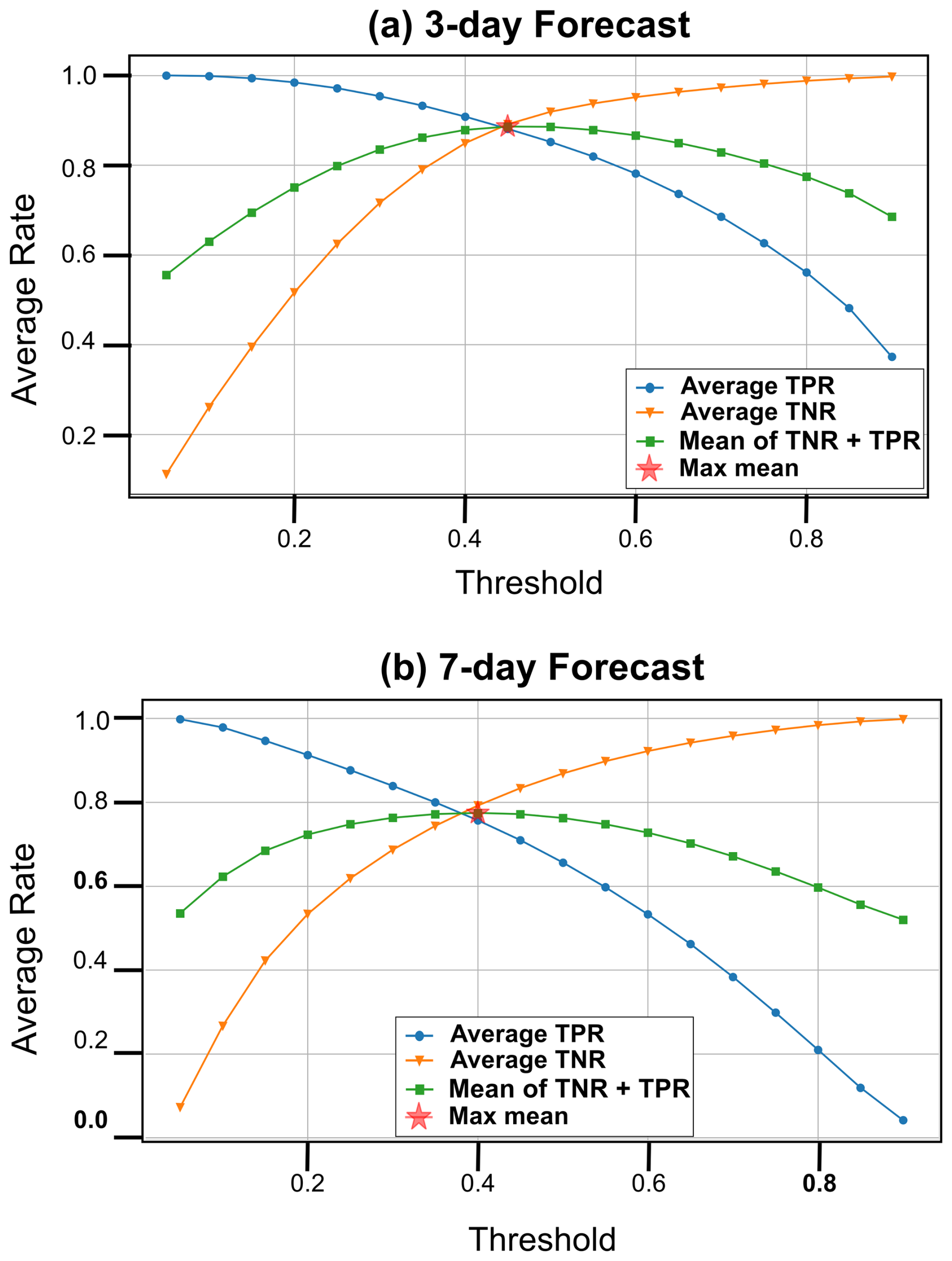
Figure 3 Threshold selection for the (a) 3 d and (b) 7 d forecast scenario based on the maximization of the combined mean (green line) of TPR (blue line) and TNR (orange line). The threshold increments range from 0.05 to 0.9, and the maximal point is indicated by a red star.

In the context of optimizing the threshold selection, TPR (Eq. 3) and TNR (Eq. 4) are prioritized over FAR (Eq. 5) as the primary goal is to accurately predict MHW occurrences (true positives) rather than minimizing false alarms (FP, FN). Given that FAR includes all grid points in the domain (128×272), it relies on a larger denominator, resulting in lower overall values. This causes the FAR curve to shift toward higher threshold values, consequently reducing the number of true positives, which is suboptimal. Nevertheless, FAR is useful as a cumulative metric and is later used to assess the spatial overall performance of the optimal model configuration.

3.2 Sensitivity analysis on input variables

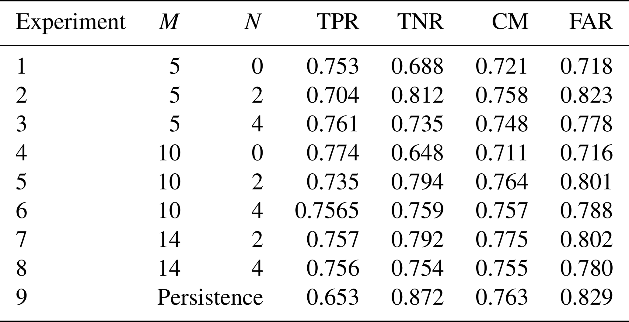
To further optimize the configuration of our U-Net CNN, we perform a sensitivity analysis on the input variables employed in training the model. Specifically, nine distinct experiments are examined for both the 3 and 7 d forecast scenarios, in which we varied the number of SSTA days and MHW presence/absence window preceding the target prediction date. The number of experiments was primarily limited by the memory constraints of our computational setup during training. Additionally, we prioritized simplicity to ensure minimal requirements during forecasting, enhancing the tool's practicality as a viable alternative for MHW prediction. For each experiment, we evaluate the corresponding TPR, TNR, CM, and FAR metrics and determine the best-performing setup of our model based on the maximum CM. The decision to prioritize CM (over FAR) reflects the greater influence of TPR on CM, aligning with our primary objective of accurately predicting positive MHW occurrences.

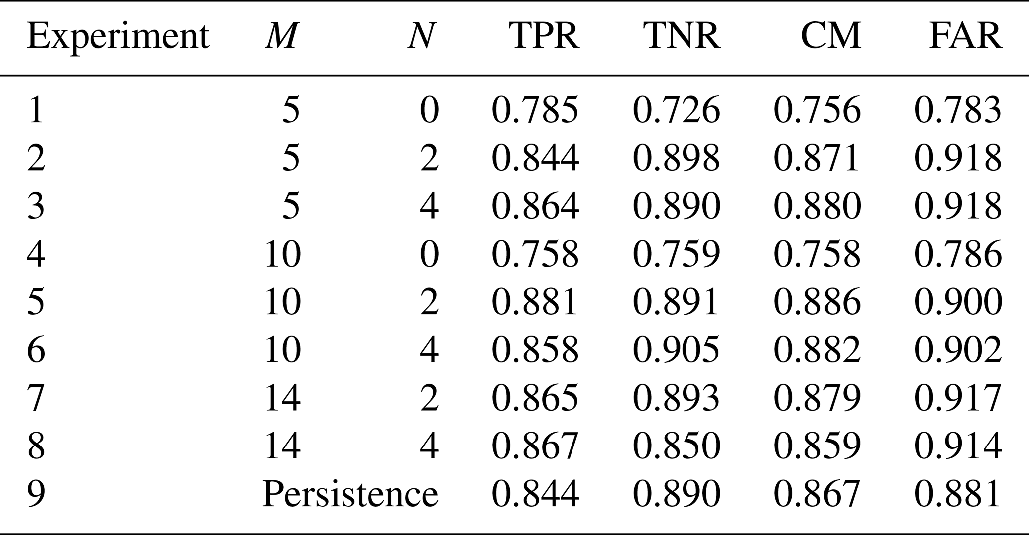
In the case of the 3 d forecast scenario, experiment 5 achieves the highest CM, incorporating M=10 preceding time steps of SSTA and N=2 preceding time steps of MHW presence/absence maps as input variables, with a total of 31 926 629 parameters trained (Table 1). Although this experiment demonstrates the highest TPR (0.881) and the second-highest TNR (0.891) among all experiments, it does not yield the maximum FAR, which is observed in experiments 3 and 2. Overall, the TPR and TNR variations across most of the sensitivity tests in the 3 d forecast scenario remain within a 5 % range, indicating a relative stability of the model's performance and robustness to small changes in input variables. However, a marked deterioration in performance is observed in experiments 1 and 4, with a TPR declining by up to 16 % compared to other experiments. This is due to the SSTA being the sole input variable (N=0) of this configuration.

Table 1 Sensitivity experiments on the input variables of the U-Net CNN model and the associated prediction metrics for the 3 d forecast scenario. The input variables configuration for each experiment is indicated with the number of preceding time steps of SSTA (N) and the number of preceding time steps (M) of MHW presence/absence maps. The highest evaluation metrics are highlighted in bold for clarity. The TPR, TNR, CM, and FAR represent true positive rate, true negative rate, combined mean, and forecast accuracy rate, respectively.

In comparison, the 7 d forecast produces slightly reduced metrics, indicating decreased accuracy over the extended forecast period (Table 2). In particular, the highest CM is identified in experiment 7, which incorporates M=14 preceding time steps of SSTA and N=2 preceding time steps of MHW presence/absence maps as input variables. While this experiment demonstrates a balanced performance, achieving a TPR of 0.757 and the second-highest TNR (0.792), experiment 9 (the persistence benchmark) exhibits the highest TNR (0.872) and a significantly lower TPR (0.653).

Compared to the 3 d forecast, the TPR and TNR variations across the sensitivity tests of the 7 d forecast reach up to 14 % (Table 2). For instance, TPR ranges from 0.653 in experiment 9 to 0.774 in experiment 4, while TNR ranges from 0.648 in experiment 4 to 0.872 in experiment 9. When excluding cases that lack MHW presence/absence maps as an input variable (N=0), the results show the same model stability (Table 1), with TPR and TNR variations confined within a 5 % range. Indeed, a marked deterioration in performance is observed in experiments 1 and 4, with TPR values ranging between 0.753 and 0.774 and TNR values between 0.688 and 0.648, respectively. This indicates that the model has limited ability to effectively draw upon patterns from past events when information about MHW presence/absence maps is excluded.

Table 2 As in Table 1 but for the 7 d forecast scenario.

3.3 Performance of optimized U-Net CNN configuration

In the following, we assess the forecasting ability of our U-Net CNN model based on the best-performing configurations of each forecast horizon. Specifically, we assess the predictive capability of experiment 5 for the 3 d forecast scenario and experiment 7 for the 7 d forecast scenario, which were determined to yield the highest performance metrics.

3.3.1 Forecast rates

The performance of the binary MHW classification is evaluated across the entire testing dataset (mid-2013 to 2017), irrespective of temporal or spatial variations, using a confusion matrix. This tool quantifies the percentage of correctly and incorrectly classified grid points within the MHW spatial domain throughout all the samples of each forecast scenario, providing a comprehensive evaluation of the model's predictive accuracy and robustness. The classification metrics used include the TPR and TNR and the false positive rate (FPR) for negative cases misclassified as positive and the false negative rate (FNR) for positive cases misclassified as negative, which are the complementary metrics to the TPR and TNR, respectively.

The model achieves high accuracy in correctly classifying both the MHW-affected (true positive) and the non-MHW grid points (true negative) in the 3 d forecast scenario, with success rates of 88.1 % and 89.1 %, respectively (Fig. 4a). Incorrect predictions account for only up to 12 % of the samples. In comparison, relatively lower rates of TPR (75.7 %) and TNR (79.2 %) are seen in the 7 d forecast (Fig. 4b), likely due to the reduced autocorrelation of the 7 d lagged input maps, compared to the 3 d case, with the proportion of misclassified cases increasing to 24 %.

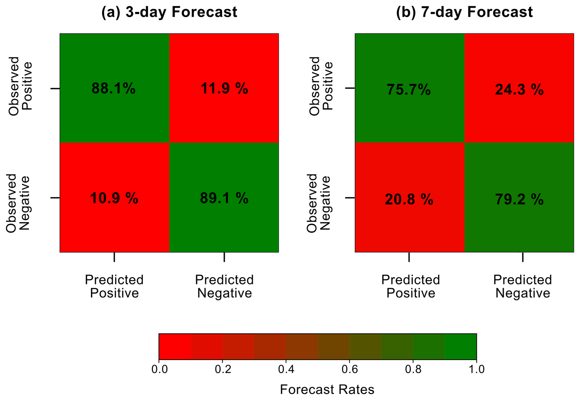
Figure 4 Confusion plot for the (a) 3 d and (b) 7 d forecast, showing the TPR (observed positive–predicted positive), TNR (observed negative–predicted negative), FPR (observed negative–predicted positive) and FNR (observed positive–predicted negative). Forecast rates are denoted in percentages within the boxes, taking into account all the samples of the testing dataset spanning mid-2013 to 2017.

To complement the analysis of aggregate metrics, we further examine the predictive accuracy of our U-Net CNN on a sample-by-sample basis within the testing dataset, spanning mid-2013 to 2017 (Fig. 5). Specifically, we compare the total number of predicted positive MHW grid points to the observed positives for each sample. By examining the alignment of data points with the line of parity (Y=X), we assess not only overall predictive skill but also patterns of systematic overprediction or underprediction within the dataset. This approach enables us to discern deviations from perfect agreement and provides insights into potential biases in the forecasts. For the 3 d forecast, a strong agreement is observed between the predicted and observed MHW occurrences as 99.31 % of the points fall within a tolerance of 3500 grid points from the Y=X line (Fig. 5a). This tolerance threshold was empirically determined to optimize performance in the 3 d forecast scenario, enabling meaningful comparisons with the 7 d forecast. Given that in geospatial analysis it is common to use a threshold based on a percentage of the total dataset to ensure stability and scalability (Xu et al., 2024), we chose a tolerance that represents approximately 10 % of the total grid points in each map. In contrast, the 7 d forecast scenario shows reduced alignment, with 86.68 % of samples meeting the same tolerance threshold. Furthermore, most points lie above the Y=X line, indicating a potential overestimation of MHW presence in this scenario (Fig. 5b).

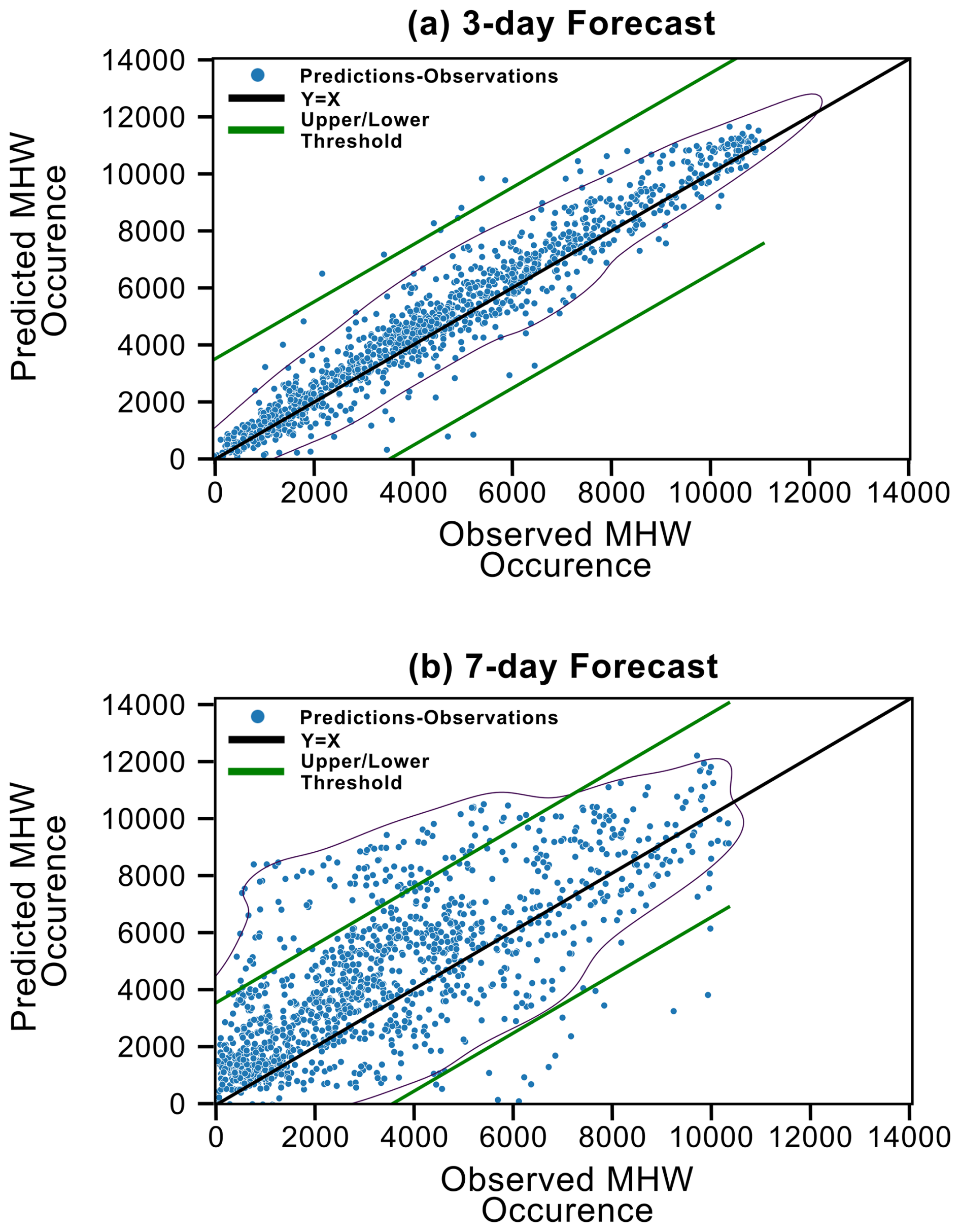
Figure 5 Scatter plots of the total number of observed (x axis) vs. predicted (y axis) points classified as MHW present (blue dots) per sample, for the (a) 3 d and (b) 7 d forecast throughout the entire testing dataset spanning mid-2013 to 2017. The upper and lower thresholds of 3500 points (green lines) are introduced for comparison purposes (see text).

These results highlight the ML model's diminished predictive reliability at extended forecast horizons, which is consistent with the inherent trade-offs in balancing sensitivity and specificity.

3.3.2 Comparison with the persistence benchmark

The final phase of evaluating the U-Net CNN configuration focuses on comparing its performance to the persistence benchmark model, which predicts MHW presence/absence based on lagged correlations over 3 and 7 d intervals (Fig. 6). The persistence model predicts MHW occurrence based on past observations, assuming that the most recent conditions are the best predictor of future events. The “noisy” TPR fluctuations observed across the test dataset can arise from rapid changes in the MHW presence/absence maps, which challenge the predictive stability of both models. This variability is further compounded in the U-Net CNN by the inherent stochasticity in neural network predictions. However, in terms of the average TPR, the U-Net CNN consistently outperforms the persistence benchmark across both forecast scenarios (Fig. 6). For the 3 d forecast, the persistence model achieves an average TPR of 0.844 (Fig. 6a), which declines to 0.653 in the 7 d forecast (Fig. 6b), reflecting stronger performance in the shorter forecast horizons. In comparison, the reduction in TPR between the 3 and 7 d forecast is less pronounced for the U-Net CNN, declining from 0.881 to 0.757. This indicates that the U-Net CNN exhibits a comparatively higher stability in maintaining predictive performance over longer forecast horizons. Overall, the best-performing experiments of the U-Net CNN outperform the persistence benchmark model, achieving higher values across all evaluation metrics in the 3 d forecast and in some select metrics for the 7 d forecast. This reflects the model's robustness in shorter forecast horizons and its ability to maintain competitive performance despite the challenges posed by longer forecast horizons.

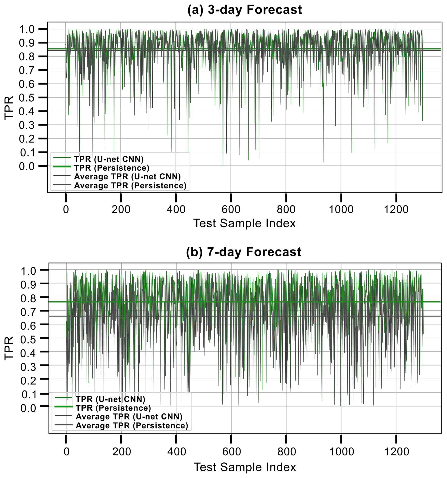
Figure 6 TPR values of each sample across the entire 3.5-year test dataset spanning mid-2013 to 2017 for the best-performing experiment and persistence benchmark of the (a) 3 d and (b) 7 d forecast. The TPR values of each U-Net model are indicated in green lines, whereas TPR of the persistence model is shown in black. The averaged value across the entire 3.5-year test dataset is also shown with the same colours as a bold line, indicating our U-Net method to be better overall.

3.3.3 Evaluation of spatial prediction accuracy

This section investigates the regions of the Mediterranean Sea displaying higher and lower susceptibility to prediction errors in our method. To this end, we examine the spatial distribution of the averaged FAR across all samples of the testing dataset (mid-2013 to 2017) for both forecast scenarios. This metric provides a cumulative assessment of the U-Net CNN model's predictive performance, enhancing our understanding of regional prediction reliability, while guiding model refinements to improve forecast precision in identified areas of weakness.

Overall, the spatial distribution of FAR reveals significant differences between the 3 and 7 d forecast scenarios. In the 3 d forecast, FAR values exceed 90 % in the northwest Mediterranean, Adriatic, and Ionian seas, as well as the southeast Mediterranean basin, as opposed to the Balearic Islands, Alboran, and Aegean seas, where slightly lower FAR values (80 %–90 %) are displayed (Fig. 7a). In the 7 d forecast, FAR values are generally lower across the entire Mediterranean Sea. Specifically, the FAR values in the Aegean Sea, the coastal areas of the northern Mediterranean basin, and the Alboran Sea range between 60 % and 70 %, with only the Ionian and Tyrrhenian seas as well as the Levantine Basin displaying FAR values approximately between 80 % and 92 % (Fig. 7b).

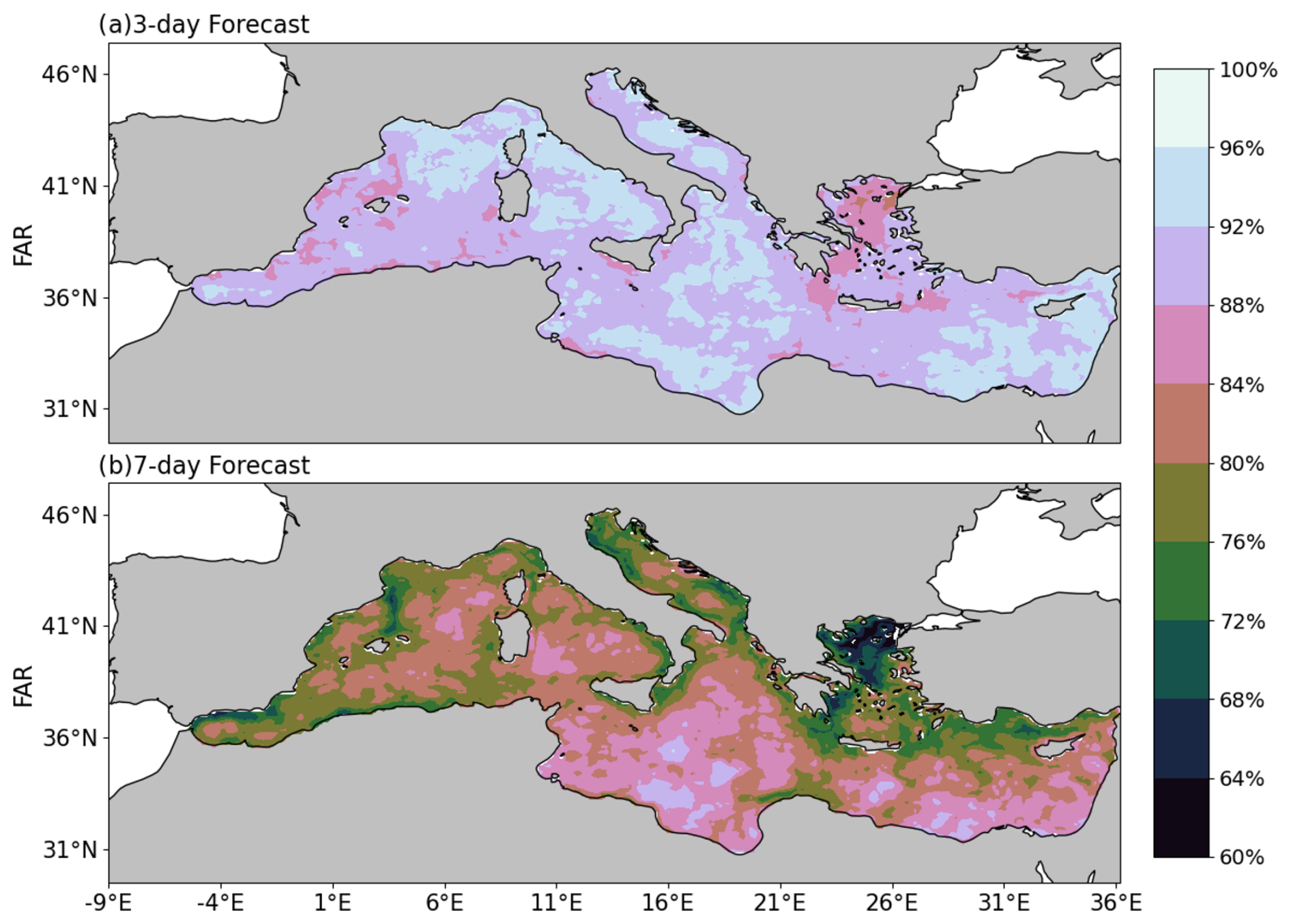
Figure 7 Spatial distribution of the forecast accuracy rate (FAR) in the Mediterranean Sea for the (a) 3 d and (b) 7 d forecast scenario, averaged across all samples of the testing dataset spanning mid-2013 to 2017.

4 Discussion and conclusions

This study presents the application of an attention U-Net CNN to predict the spatiotemporal evolution of MHWs in the Mediterranean Sea. The proposed model integrates an attention mechanism with a standard U-Net architecture, combined with a focal binary cross-entropy loss function, among other key parameters. The model is trained on SSTA and information on daily MHW presence/absence between 1982 and 2017 to predict future MHW occurrence within 3 and 7 d forecast horizons. Extensive hyperparameter tuning is carried out to ensure the model's stability and performance within acceptable limits alongside the implementation of a specific threshold selection technique. The results, presented for both forecast horizons, highlight a decline in forecasting skill as the prediction horizon increases, with our U-Net CNN consistently outperforming the persistence benchmark model.

For the optimal thresholding technique of MHW probability, we prioritize the accurate detection of true MHW instances (TPR) over minimizing the number of non-MHW instances (TNR). Specifically, we focus on the maximization of the combined mean of TPR and TNR (CM) to ensure a balance between sensitivity and specificity (Sun et al., 2023). As the threshold increases, a trade-off emerges between the TPR and TNR (green line, Fig. 3), whose curves form a concave shape with a distinct maximum point. In cases where this maximum is not well defined, an optimal threshold can be determined either empirically (Fawcett, 2006), based on the intersection of TPR and TNR (Fig. 3), or by maximizing the FAR metric (Sun et al., 2023).

The optimal configuration of the U-Net CNN is then determined through sensitivity analysis, assessing the impact of various input variable combinations on model performance. The best-performing configuration incorporates M=10 preceding SSTA time steps and N=2 preceding time steps of MHW presence/absence for the 3 d forecast (Table 1) and M=10 and N=4 for the 7 d forecast (Table 2). In both forecast scenarios, configurations relying solely on SSTA data demonstrate the weakest performance, highlighting the importance of integrating both temperature anomalies and prior MHW occurrences to achieve more reliable forecasting of these events. Particularly for the 7 d forecast, the variations in the CM and FAR metrics across the different experiments are less pronounced when excluding experiments with a single input variable. In line with the findings of Sun et al. (2023), this sensitivity analysis aims to optimize the model's performance on unseen data while maintaining simplicity for future end users and balancing model complexity and generalization.

However, the assessment of the U-Net CNN's forecast ability reveals distinct differences in predictive accuracy between the short-term (3 d) and longer-term (7 d) forecast horizon. While the 3 d forecast achieves the highest average TPR and TNR metrics overall, its discrepancy relative to the persistence benchmark is modest, potentially due to the high autocorrelation of the SSTA in both the benchmark and the 3 d forecast (Fig. 6a). In contrast, the 7 d forecast exhibits lower TNR and TPR values, with the performance gap between the benchmark and the U-Net CNN being more pronounced (Fig. 6b). Thus, our results indicate an improved accuracy in shorter forecast horizons, in agreement with Bonino et al. (2024). Despite demonstrating a decline in TPR from the 3 d to the 7 d forecast scenario, the strength of the U-Net CNN lies in maintaining a higher TPR value than the persistence benchmark in both forecast scenarios, suggesting an improved ability to predict MHWs across different temporal scales.

Based on the FAR metric, an improved forecasting performance (high FAR values) of the U-Net CNN is revealed in the northwest Mediterranean basin, the Ionian Sea, and the Levantine Basin as opposed to the lower FAR values observed in the Aegean and Alboran seas, Balearic Islands, and northern coastal areas (7 d forecast). In the case of the Aegean Sea, the low FAR values may reflect challenges in detecting MHWs due to rapid SST fluctuations influenced by the Black Sea. These fluctuations can lead to swift onset and dissipation of MHWs (Mavropoulou et al., 2016), complicating their detection by ML methods. Additionally, the downsampling applied to address the high computational demands of our method (see Sect. 2.2) resulted in a reduced spatial resolution of the data. This reduction likely affected the model's performance in regions with complex topography, such as the Aegean Sea and coastal areas. This is likely due to the reduction in spatial resolution (halved to 12–16 km) near the coast, which results in the averaging of values and the loss of high-resolution information in these regions. While we acknowledge this limitation, we prioritize reliable forecasting of MHWs across the entire Mediterranean Sea, understanding that higher-resolution models, though more accurate in these areas, also come with increased computational demands. This is also observed in Bonino et al. (2024), where the authors also report a reduced forecast ability of their neural network model around the Adriatic Sea, Balearic Islands, and the Alboran and Aegean seas. Given that ocean circulation along the coast is primarily driven by local winds and can be influenced by offshore currents near complex topographic features, the exclusion of winds as an input dataset may have further reduced the forecast accuracy of our ML model in shallow coastal areas, where SST variations become more complicated (Berthou et al., 2024; Liu et al., 2025). However, Bonino et al. (2024) found a weak dependence of the SST on wind speed across all the Mediterranean sub-basins they considered by calculating the mutual information index prior to applying the ML method. While incorporating atmospheric variables into the training process could thus potentially enhance the model's ability to capture broader climatic influences on MHW occurrence, ultimately, we selected a limited set of training variables in order to enhance the model's simplicity and replicability across both the training and prediction phases following Sun et al. (2023).

It is important to note that the results of this study are based on the “straight split” methodology, where the early years of the dataset are used for training and the final years for testing. Given that ML models trained on recent data often achieve higher accuracy due to the influence from recent climate patterns (recency effect; Lam et al., 2023), we have also explored the impact of reversing the training and testing dataset order. In particular, we carried out a sensitivity test, defined as the opposite split, using the years 2013–2017 for training and 1982–1986 for testing to assess whether our model's predictive skill is dataset-dependent or driven by climate-change-induced temperature (see Table S1). For the 7 d forecast horizon, we find improved TNR and TPR metrics when more recent data are inserted in the training dataset. This aligns with the findings of Lam et al. (2023), where recent climate trends, including the increased frequency of MHWs, were shown to enhance model effectiveness by mitigating issues of data scarcity and imbalance in the training datasets. However, for the 3 d forecast, we find a deterioration of both metrics, compared to the outputs of the straight split methodology (see Table S1 in the Supplement). This may be due to the longer duration of recent MHWs, which are less frequent in earlier years (Oliver et al., 2018) and thus may be poorly represented in the training dataset. In this study, we thus used the straight split methodology as the training of a neural network with historical data to forecast information in the future reflects a more realistic approach.

Overall, the proposed U-Net CNN model offers a computationally efficient alternative to traditional regional forecasting models for predicting MHWs in the Mediterranean Sea. Once trained, our approach maintains high spatiotemporal resolution while requiring minimal computational resources. The results indicate that the model performs better in the 3 d forecast compared to the 7 d forecast across all evaluation metrics and relative to the persistence benchmark. This outcome is expected given the higher autocorrelation of SSTAs over shorter time frames, which is consistent with other studies such as Sun et al. (2023) and Taylor and Feng (2022). Although the 7 d forecast holds greater practical value for the early prediction of extreme events, enabling more effective mitigation strategies, it remains a challenging task for ML methods, as reflected in the lower persistence benchmark values over longer time horizons. In comparison, the 3 d forecast achieves higher overall metrics due to the shorter forecasting window and the inherently higher persistence benchmark values. Nevertheless, the U-Net model still outperforms the benchmark in the 3 d forecast, albeit by a smaller margin than in the 7 d forecast. Given the model's success in predicting MHWs using a minimum input of variables in a region with diverse thermohaline and circulation patterns, such as the Mediterranean Sea (Benincasa et al., 2024), it is reasonable to assume that our methodology can be generalized to other basins and case studies. While a similar ML approach has demonstrated comparable forecasting performance in areas with similar data availability (Sun et al., 2023), factors such as grid size and computational resources may also influence the training process of the ML model. Notably, the primary challenge in applying the U-Net CNN for predicting MHWs in this study was achieving a balance between predictive accuracy and computational efficiency, which is an important consideration for the application of all ML methods.

As global warming accelerates, the increasing frequency and severity of MHWs pose significant challenges to marine ecosystems. Efficient and timely forecasting of MHWs is essential for effective marine management, enabling governments, industries, and coastal communities to take proactive measures, such as imposing temporary fishing bans, enhancing monitoring of vulnerable species, establishing marine protected areas, and launching public awareness campaigns to promote sustainable practices. ML-based approaches show promise for improving predictions of these events, particularly through architectures like the attention U-Net CNN employed in this study, which reconstruct spatially distributed variables and generate high-resolution predictions within seconds to minutes, depending on available computational resources. This rapid forecasting ability is particularly advantageous for short-term predictions as climate models typically require days of runtime and data assimilation to achieve comparable accuracy in operational settings (Coppini et al., 2023). For instance, a significant computational benefit was demonstrated using a neural-network-based regional climate model (RCM) emulator that was trained to reproduce complex spatial structure and variability in near-surface temperature simulated by an RCM (Doury et al., 2023). By learning the relationship between the low-resolution predictors and high-resolution surface variables over the RCM domain, this approach enables the low-cost generation of high-resolution RCM simulation ensembles, which are useful for exploring local-scale uncertainties in present and future climate.

As computational capabilities advance, ensemble models, such as those used in time series regression (Bertsimas and Boussioux, 2023) could also improve CNN-based forecasting of MHWs, especially for long-term model predictions that are typically hindered by error propagation. Future research should consider training ML models on observed or remotely sensed data, despite their limitations (Abdelmajeed and Juszczak, 2024), as well as hybrid approaches that combine the physical consistency of traditional models with the speed and adaptability of ML methods (Bonino et al., 2023). Given that the accuracy and reliability of many ML models is compromised by their violation of fundamental physical principles (Chen et al., 2023), future efforts should also focus on addressing this limitation by incorporating physical laws (Desai and Strachan, 2021) or analytical equations (Zanetta et al., 2023), which are approaches that, though in early stages, show promise.