Internal-wave-induced dissipation rates in the Weddell Sea Bottom Water gravity current

This study investigates the role of wave-induced turbulence in the dynamics of the Weddell Sea Bottom Water gravity current. The current transports dense water from its formation sites on the shelf to the deep sea and is a crucial component of the Southern Ocean overturning circulation. The analysis is based on velocity records from a mooring array deployed across the continental slope between January 2017 and January 2019 as well as vertical profiles of temperature and salinity measured on various ship expeditions on a transect along the array. Previous studies suggest that internal waves may play a crucial role in driving turbulence within gravity currents; however, this influence has not been quantitatively assessed. To quantify the contribution of internal waves to turbulence in this particular gravity current along the continental slope, we employ three independent methods for estimating dissipation rates. First, we use a Thorpe scale approach to compute total, process-independent dissipation rates from density inversions in density profiles. Second, we apply the fine-structure parameterization to estimate wave-induced dissipation rates from vertical profiles of strain, calculated from temperature and salinity profiles. Third, we estimate wave energy levels from moored velocity time series and deduce wave-induced dissipation rates by applying a formulation that is at the heart of the fine-structure parameterization. Turbulence is highest at the shelf break and decreases towards the deep sea, in line with decreasing strength of wave-induced turbulence. We observe a two-layer structure of the gravity current, a strongly turbulent bottom layer about 60–80 m thick, and an upper, more quiescent interfacial layer. In the interfacial layer, internal waves induce an important part of the dissipation rate and therefore drive entrainment of warmer upper water into the gravity current. A precise quantification of the contribution is complicated by large method uncertainties. A comparison with turbulence measurements up- and downstream of our study site indicates that the processes dominating turbulence generation may depend on the location along the Weddell Sea Bottom Water gravity current: on the shelf trapped waves are most important, on the continental slope breaking internal waves dominate, and in the basin symmetric instability is likely the main driver of turbulence.

1 Introduction

The global overturning circulation is closed through deepwater formation at high latitudes, connecting surface and deep-sea currents. Nearly half of the circulation's densest water mass, the Antarctic Bottom Water, originates in the Weddell Sea (Hellmer and Beckmann, 2001). This gives the Weddell Sea, a marginal sea in the Southern Ocean (Fig. 1a), a critical role in global ocean and climate dynamics. A combination of processes on the continental shelves of the southern Weddell Sea produces the world ocean's densest water (Foldvik et al., 2004). The most important processes are marine heat loss to the atmosphere during sea ice formation and melting of ice shelves from below. The newly formed water mass, often referred to as Dense Shelf Water, flows as a gravity current down the continental slope (Llanillo et al., 2023). Steered by the Coriolis force, the current follows the Antarctic continental shelf (Fig. 1b). The water mass transported by the gravity current is referred to as Weddell Sea Bottom Water (WSBW). We use the framework of neutral density (Jackett and McDougall, 1997) here and define WSBW as water of neutral density with γⁿ>28.40 kg m⁻³ (Naveira Garabato et al., 2002b; Meredith et al., 2008; Dotto et al., 2014; Llanillo et al., 2023) because it automatically excludes very cold surface waters (Fig. 2).

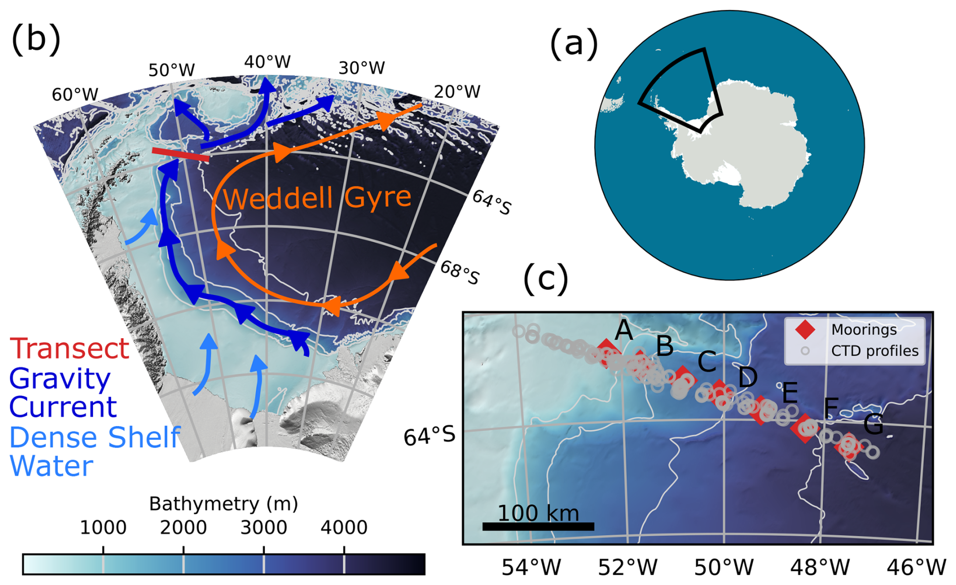
Figure 1 Geographical overview. (a) Location of the Weddell Sea in the Southern Ocean. (b) Map of the Weddell Sea, with the Joinville transect across the continental slope in red. Light blue arrows show the paths of Dense Shelf Water, which feed the Weddell Sea Bottom Water gravity current, shown in dark blue. Light gray lines are isobaths in steps of 1000 m. (c) Map of the Joinville transect across the continental slope. Moorings are named A to G from west to east (Table 2). Light gray lines are isobaths in steps of 1000 m.

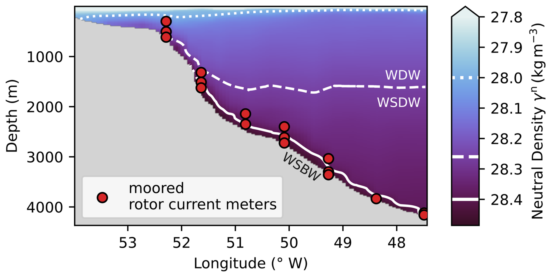
Figure 2 Neutral density γⁿ transect across the continental slope, with the Antarctic Peninsula to the west. Density has been horizontally interpolated from CTD profiles, measured during the PS129 expedition. Isopycnals at γⁿ=28.00, 28.26, and 28.40 kg m⁻³ denote water mass boundaries (AASW–WDW, WDW–WSDW, and WSDW–WSBW). Weddell Sea Bottom Water (WSBW) is located along the slope. Red circles show rotor current meter locations.

An important property of WSBW is that it is too dense to leave the Weddell Sea except in small volumes through the deepest passages (Naveira Garabato et al., 2002a). The majority of the water leaving the Weddell Sea to become Antarctic Bottom Water is provided by Weddell Sea Deep Water (WSDW), which is categorized to have a neutral density of 28.26 kg m${}^{-\mathrm{3}}<{\mathit{\gamma }}^{\mathrm{n}}<\mathrm{28.40}$ kg m⁻³ (Naveira Garabato et al., 2002b). It is formed through mixing processes of Weddell Sea Bottom Water with ambient lighter waters (Nicholls et al., 2009). Above the WSDW, Warm Deep Water (WDW) extends up to the γⁿ=28.00 kg m⁻³ isopycnal (Naveira Garabato et al., 2002b), which separates it from the overlying Antarctic Surface Water (AASW) (Fig. 2).

The physical properties of Antarctic Bottom Water exported from the Weddell Sea are thus in part determined by processes at the formation sites on the continental shelves, but also by entrainment of upper, less dense water into the WSBW gravity current during its passage down the continental slope. This entrainment of ambient water is a consequence of mixing by multiple turbulent processes. Investigating the role and nature of the small-scale processes involved in the entrainment is therefore essential for advancing our understanding of Antarctic Bottom Water formation (Silvano et al., 2023, Question 7). This further understanding is especially needed as Antarctic Bottom Water has been observed to warm and freshen (Purkey and Johnson, 2013) at increasing rates (Menezes et al., 2017; Johnson et al., 2019) and is hypothesized to be a potential tipping point in the global climate system (Lenton et al., 2008). Global and regional numerical ocean models cannot resolve the scales of vertical mixing required for simulating realistic deepwater formation (Legg et al., 2009) and have to rely on parameterizations (Heuzé, 2021). For the development and constraint of these parameterizations, and to understand turbulent entrainment into dense gravity currents, an observation-based approach is necessary.

Many turbulent processes found in gravity currents are driven by the kinetic energy of the gravity current itself, like shear instabilities at the interface to the ambient water or friction and drag at the seafloor (Legg et al., 2009). However, only considering this driving mechanism would leave out the ever-present external energy source of internal waves. While turbulence driven by breaking internal waves is the most important mixing mechanism in the open ocean and accordingly discussed in many publications (Meredith and Naveira Garabato, 2022, and references therein), the interaction of internal waves and gravity currents is only studied in few publications (e.g., Peters and Johns, 2006; Seim and Fer, 2011; Nash et al., 2012), some of which consider only very idealized setups (Hogg et al., 2018; Tanimoto et al., 2021, 2022). Multiple works (Peters and Johns, 2006; Umlauf and Arneborg, 2009; Seim and Fer, 2011; Schaffer et al., 2016) conclude that wave-induced turbulence may be important for entrainment into gravity currents but without further quantitative analysis of wave contribution. We hence aim to evaluate and quantify the importance of wave-induced turbulence for the WSBW gravity current.

The Weddell Sea features strong tidal currents (Foldvik et al., 1990; Levine et al., 1997; Robertson et al., 1998), suggesting a vigorous internal wave field produced by their interaction with rough topography. But at the same time, the Weddell Sea has repeatedly not been included in global maps of internal wave energy (Waterhouse et al., 2014; de Lavergne et al., 2019; Pollmann, 2020; Pollmann et al., 2023) due to its remote and difficult-to-access location at high latitudes. Our research is based on the Joinville transect (as part of the Go-Ship line SR04) across the Antarctic continental slope, which covers the pathway of the WSBW gravity current in the northwestern Weddell Sea before it exits into the deep sea. We use shipboard observations of salinity and temperature from 13 cruises, one of which collected coincident velocity profile data, and approximately 2 years of moored velocity, salinity, and temperature data to quantify turbulence dependent on its driving energy source from three independent methods:

1. a Thorpe scale approach applied to vertical profiles,

2. a parameterization based on the energy contained in internal waves, and

3. strain-based fine-structure parameterization from vertical profiles.

We obtain the contribution of wave-induced turbulence to the overall turbulence by horizontal and vertical comparison of the results from all three methods. From this, we can assess the relevance of internal waves for entrainment of ambient water into the WSBW gravity current.

2 Data

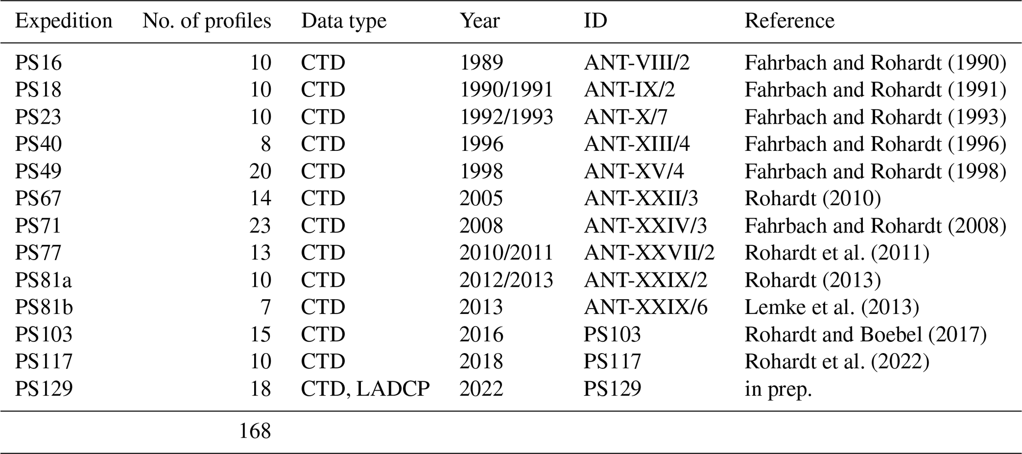
This study is based on multiple observations along a transect across the continental slope east of the Antarctic Peninsula (Fig. 1c). This section briefly describes mooring data and hydrographic conductivity, temperature, and depth (CTD) profiles along the transect. We use salinity and temperature data from 13 expeditions between 1989 and 2022, undertaken by RV Polarstern (Knust, 2017), which collected 168 CTD profiles along the Joinville transect (Table 1). Profiles from other RV Polarstern expeditions to the same region are rejected, as they measured along a different transect that is offset from the one we consider. This is done to keep the CTD profiles spatially comparable in the cross-section along the continental slope. Due to the prevalent sea ice conditions of the region, the CTD profiles are not evenly distributed across the year but strongly biased to the austral summer, with 143 out of 168 profiles measured between November and April. Five CTD profiles stand out as outliers and are subsequently removed as nonphysical profiles from the data analysis, as they differ by many standard deviations from the mean background stratification. Profiles are depth-binned at 1 or 2 dbar resolution following standard procedures to reduce measurement noise and errors due to ship movement. The CTD measurements are accurate to 0.002 °C in temperature and 0.002 g kg⁻¹ in salinity, which results in a density resolution of similar magnitude of 10⁻³ kg m⁻³. During expedition PS129, the CTD rosette was also equipped with lowered acoustic Doppler profilers (LADCPs). The measured velocity profiles have a vertical resolution of 10 m.

Fahrbach and Rohardt (1990)Fahrbach and Rohardt (1991)Fahrbach and Rohardt (1993)Fahrbach and Rohardt (1996)Fahrbach and Rohardt (1998)Rohardt (2010)Fahrbach and Rohardt (2008)Rohardt et al. (2011)Rohardt (2013)Lemke et al. (2013)Rohardt and Boebel (2017)Rohardt et al. (2022)

Table 1 Ship-based data from RV Polarstern cruises along the transect between 1989 and 2022. The seasonal distribution of the CTD profiles is biased towards the austral summer, with 143 out of 168 profiles measured between November and April.

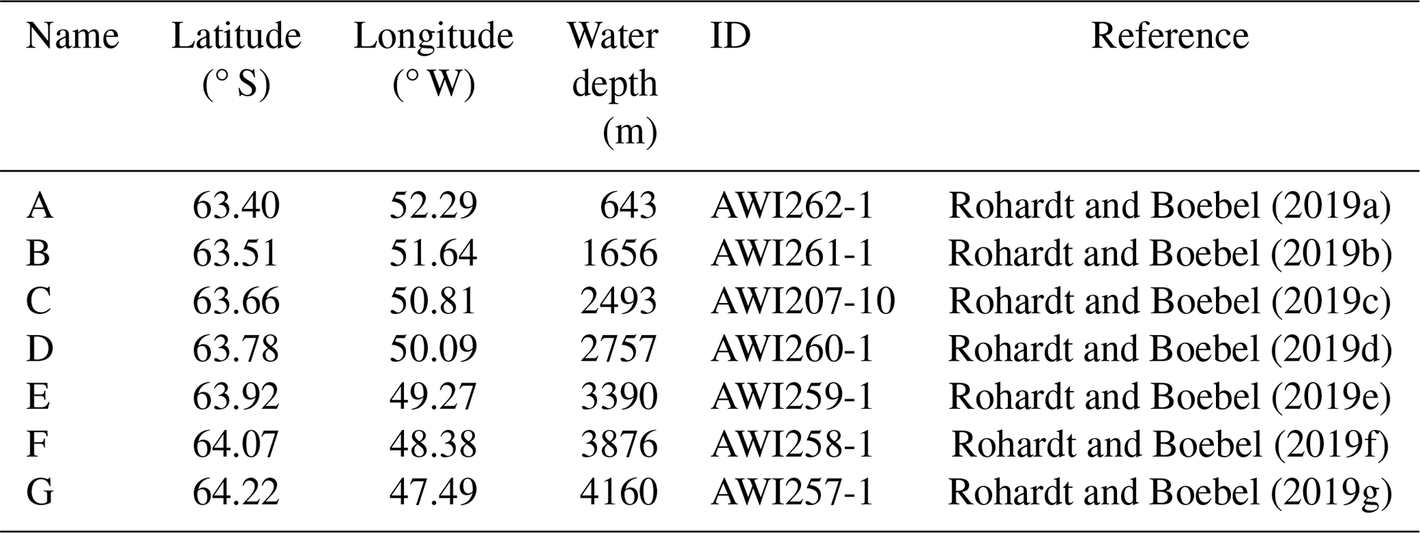
Seven moorings were deployed along the transect (Fig. 1c) during RV Polarstern expedition PS103 around New Year 2016/2017 and recovered in January 2019, during PS117. Horizontal spacing between the moorings is 35 to 50 km. The moorings were each equipped with up to three rotor current meters (RCMs) built by Aanderaa (models RCM7, RCM8, and RCM11), three Sea-Bird MicroCAT CTD sensors (SBE37), and three Sea-Bird temperature–depth recorders (SBE39/56). The RCMs had an accuracy of ±1 cm s⁻¹ for speed and ±5° for direction and integrated vector velocity over 2 h periods. Most velocity time series considered here are 2 years in total length, except for a few shorter records because of battery failure. Vertical resolution of the RCMs ranges from 50 to 200 m. More detailed information can be found in the respective cruise reports (Boebel, 2017, 2019).

Rohardt and Boebel (2019a)Rohardt and Boebel (2019b)Rohardt and Boebel (2019c)Rohardt and Boebel (2019d)Rohardt and Boebel (2019e)Rohardt and Boebel (2019f)Rohardt and Boebel (2019g)

Table 2 Moorings along the Joinville transect from January 2017 to January 2019, along with their coordinates, total water depth, official ID, and reference. From the referenced datasets we use current velocity, in situ temperature, pressure, practical salinity, time, and depth.

3 Methods

Water masses in the Weddell Sea are categorized based on neutral density γⁿ (Naveira Garabato et al., 2002b; Meredith et al., 2008; Dotto et al., 2014; Llanillo et al., 2023). Therefore, we calculate neutral densities for each CTD profile with the MATLAB toolbox eos80_legacy_gamma_n (Jackett and McDougall, 1997; Jackett et al., 2018, v3.05.10). Results are averaged arithmetically in 0.5° longitude bins to form mean background densities and are then used to differentiate between water masses. Gravity current mean flow is calculated by taking long-time averages of absolute values over the complete measurement period for each complex horizontal velocity time series u+iv. The produced data points are interpolated linearly, first vertically then horizontally, to yield an approximate mean flow field.

Our main goal is to quantify turbulence in the gravity current dependent on its driving energy source. The amount of turbulence is quantified by the dissipation rate ε in units of W kg⁻¹, the conversion rate of turbulent kinetic energy to heat. To do so, we apply three different methods. We first estimate the total turbulent kinetic energy dissipation by applying the Thorpe scale method to density profiles (Thorpe, 1977). Because the Thorpe scale approach does not distinguish between overturns produced by breaking internal waves, instabilities, or other sources, it gives an estimation of the total dissipation rate. We then calculate the internal-wave-induced turbulence with two methods based on evaluations of spectral energy transfers by wave–wave interactions (Olbers, 1976; McComas and Müller, 1981; Henyey et al., 1986): one of them is the standard, strain-based fine-scale parameterization (Gregg, 1989; Wijesekera et al., 1993; Polzin et al., 2014, and references therein) applied to the observed CTD profiles, and the other is based on energy levels directly, which we obtain here from the observed velocity time series, as in the internal wave model IDEMIX (Olbers and Eden, 2013). The methods are described in detail in the following subsections. All dissipation rate results will be compared horizontally and vertically to obtain the contribution of internal wave breaking to the overall dissipation rates.

3.1 Total dissipation rate estimates from Thorpe scales

Total dissipation rates of turbulent kinetic energy are inferred from potential density profiles by analyzing Thorpe scales (Thorpe, 1977), meaning the mean sizes of the energy-containing overturns (Fernández Castro et al., 2022). This vertical scale is defined inside an unstable segment as the root mean square of the required vertical displacement of water parcels to form stable stratification. The Thorpe length scale L_T is linearly related to the Ozmidov scale L_O, at which buoyancy becomes important for eddies (Dillon, 1982; Crawford, 1986; Ferron et al., 1998). If both scales reach similar lengths, the overturns efficiently interact with buoyancy forces and transport mass against the stratification, i.e., pushing lighter water down and/or bringing denser water up (Fernández Castro et al., 2022). The Ozmidov scale is calculated as $L_{\mathrm{O}}={\mathit{\epsilon }}^{\mathrm{1}/\mathrm{2}}{N}^{-\mathrm{3}/\mathrm{2}}$ (Dillon, 1982), dependent on dissipation rate ε in units of W kg⁻¹, the conversion of turbulent kinetic energy to heat, and the buoyancy frequency N in units of rad s⁻¹, describing the vertical stratification.

The overturns, deviations from a stable water column, can be the result of any turbulent event, making this approach blind to the exact process leading to turbulence. Therefore, the dissipation rate ε in the Ozmidov scale definition equals the total dissipation rate ε_total. This distinction is important, as other methods for quantifying turbulence applied later in this study are not process-independent. The linear relation between the Ozmidov and Thorpe scale is defined empirically and slightly varies between studies (Dillon, 1982; Ferron et al., 1998; Voet et al., 2015) but remains close to 1. Because we lack observations to compare results of the Thorpe scale approach to direct turbulence measurements, here we refer to the literature value of L_O=0.8L_T, which is also used in Thorpe scale analysis of a dense water overflow in Storfjorden, located at high latitudes (Fer et al., 2004). This value is comparable to the choice of 0.76 by North et al. (2018) for their study of the Denmark Strait overflow. This results in the relation

$$\begin{array}{}\text{(1)}& {\mathit{\epsilon }}_{\mathrm{total},\mathrm{Thorpe}}={\mathrm{0.8}}^{\mathrm{2}}{L}_{\mathrm{T}}^{\mathrm{2}}{N}^{\mathrm{3}}.\end{array}$$

For each overturn, part-wise constant buoyancy frequency N is calculated, which represents an average background stratification of the hypothetical stable profile. The calculation of N is done with the Gibbs Seawater (GSW) Oceanographic Toolbox (McDougall and Barker, 2011; Firing et al., 2021), a thermodynamically consistent formulation based on the Gibbs function. The Thorpe scale method is implemented with the mixsea package for Python (Voet et al., 2023). In order to exclude spurious overturns caused by measurement noise in the profiles, we use a criterion based on a density noise value above which we can accurately resolve density differences (see Sect. 2): overturns with top-to-bottom density differences below $\mathrm{5}\times {\mathrm{10}}^{-\mathrm{4}}$ kg m⁻³ are rejected. Additionally, following Gargett and Garner (2008), any overturn where the ratio of the vertical distances above and below its inflection point is below 0.2 is rejected as nonphysical. We manually discard a single overturn (diagnosed around 48° W, ending 200 m above the seafloor), as it is several hundred meters in length, leading to unrealistic high dissipation rates.

In profile segments in which no overturns are detected, we assume for averaging purposes a background dissipation rate of 10⁻¹⁰ W kg⁻¹. As turbulence consists of a sequence of low- and high-energy events, we use an arithmetic average to estimate time-averaged dissipation rates. All profiles of total dissipation rates are averaged arithmetically inside bins of 0.5° longitude across the slope. In the vertical, we keep the resolution of the CTD profiles of 1 m. Potential systematic shortcomings of the Thorpe scales method are presented in Sect. 5.1.1.

3.2 Wave-induced dissipation rate estimates from squared wave energy

We calculate dissipation rates induced by internal gravity waves (IGWs), ε_IGW, from internal wave energy levels. The following sub-subsections will explain the steps from the measured velocity time series to horizontal kinetic energy spectra (Sect. 3.2.1), the kinetic energy distribution between tides and internal wave continuum (Sect. 3.2.2), the conversion from kinetic energy to total energy (Sect. 3.2.3), the energetic contribution of internal tides (Sect. 3.2.4), and finally the computation of wave-induced dissipation rates (Sect. 3.2.5).

3.2.1 Horizontal kinetic energy spectra from velocity time series

Internal wave energy levels are calculated from moored horizontal velocity time series u and v based on spectral methods. This approach is comparable to previous works on internal waves and their energy (van Haren et al., 2002; Polzin and Lvov, 2011; Le Boyer and Alford, 2021). The vertical velocity is assumed to be small compared to the horizontal components and is neglected. The complex horizontal velocity u+iv is viewed as the sum of clockwise and counterclockwise rotating components. Rotary spectra are calculated from complex velocity time series using the multitaper method (Thomson, 1982; Prieto, 2022). This method repeats spectral calculations of the complex time series in tapered windows and is controlled by three parameters: the time-half-bandwidth product P, the number of Slepian tapers k, and the window width. The time-half-bandwidth product P is usually called NW in the literature to reflect its factors but is renamed here to avoid doubling of variable names. The significance of P is that frequencies inside a window of 2P Fourier coefficients are smoothed. We chose a value of P=10 to balance desired frequency resolution and noise reduction. We use $k=\mathrm{2}P-\mathrm{1}=\mathrm{19}$ Slepian tapers and a window width of the full length of the velocity time series of the order of 5×10³ points. Multitaper parameters differ across the literature and fields of application (Thomson, 1982; Cokelaer and Hasch, 2017; Le Boyer and Alford, 2021). Our choices closely resemble the parameters Chave et al. (2019) use to resolve infragravity waves and tidal frequencies in deep-ocean pressure records.

Velocity spectra are divided by 2 to yield horizontal kinetic energy densities. Both rotary components are added to form spectra 𝒰(z,ω) of full horizontal kinetic energy, dependent on frequency ω and measurement depth z (see the example in Fig. 3b). The conservation of energy in the multitaper method is assured by integrating over the full energy spectra and checking the result against kinetic energy directly computed from complex velocity time series. Velocity measurements every 2 h correspond to a maximum frequency resolution of 6 cpd (cycles per day). The resulting spectra have the general shape of a plateau at low frequencies and an exponential decay towards high frequencies. On top are peaks, most pronounced at diurnal (1 cpd) and semidiurnal (2 cpd) frequencies. This is shown exemplarily in Fig. 3b for a spectrum derived from velocity time series measured at mooring B (63.51° S, 51.64° W) at a depth of 1513 m.

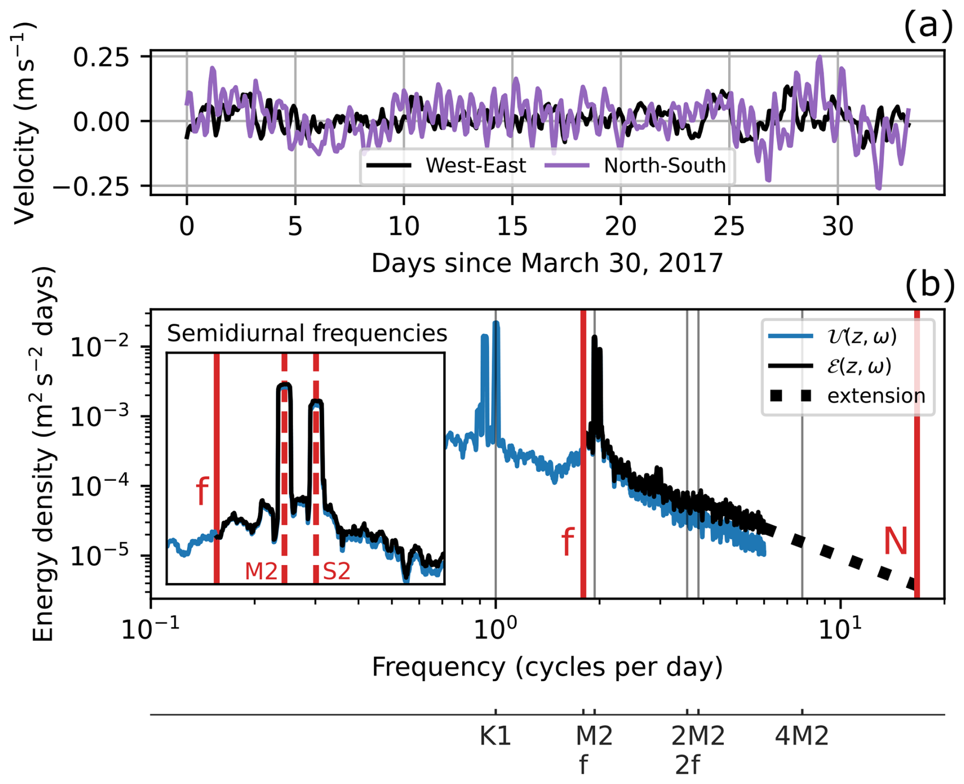
Figure 3 (a) Excerpt of a velocity time series, measured at mooring B (63.51° S, 51.64° W) at a depth of 1513 m, 143 m above ground. (b) Corresponding kinetic horizontal energy spectrum 𝒰(z,ω) in blue. The black line shows the derived total energy spectrum ℰ(z,ω) in the linear wave range. The Coriolis frequency f and buoyancy frequency N are both marked by vertical red lines. The dotted black line shows the spectral extension up to N. In the example, the slope is of a constant value of −1.9. The inset figure shows a zoomed-in view of the semidiurnal tidal frequencies, with the most prominent frequencies, M2 and S2, drawn as dashed red lines.

3.2.2 Wave energy available for local dissipation

Not all of the observed horizontal kinetic energy can be attributed to internal gravity waves. Additionally, waves contribute their energy only in part to near-field mixing. Therefore, it is necessary to clearly distinguish the underlying energy sources and transfer processes that together produce the observed horizontal kinetic energy spectra (Fig. 3b). The generation of internal waves happens at large scales, for example from interaction of (tidal) currents with the rough seafloor. Wave–wave interactions, for example parametric subharmonic instabilities (Olbers et al., 2020), wave–topography interactions, or wave–mean flow interactions (Musgrave et al., 2022), transfer the energy to ever smaller scales, where the likelihood for wave breaking increases (Falahat et al., 2014). We identify the smooth exponential decay of the background inside the frequency range of the Coriolis frequency f to buoyancy frequency N with the internal wave continuum (Munk, 1981). An attempt to find a general model for this spectrum is done in the Garrett–Munk model of the internal wave energy spectrum (Garrett and Munk, 1972, 1975). The sharp peaks in Fig. 3b are the result of overlapping depth-independent barotropic and depth-varying baroclinic tides at their respective frequencies.

The superposition of vertically propagating internal waves, reflecting repeatedly at the surface and at the bottom, can be viewed as standing vertical waves or modes. The higher the mode number, the smaller the scales, implying that the timescales of wave–wave interactions, which randomize the wave phase, and the travel times between the ocean surface and bottom become comparable (Olbers, 1983). In other words, before a standing wave can even form, the nonlinear processes have made the wave incoherent. The modal description is hence mainly useful for representing weakly dissipative waves of low mode numbers, which can transport energy over long distances (Rainville and Pinkel, 2006). Highly dissipative waves of high mode numbers are less well represented, as their traveled distance may be shorter than the distance to the next reflecting plane, e.g., the seafloor or the surface. A summary of the current state of knowledge about mixing by topographically generated internal waves is given in Musgrave et al. (2022).

Most of the energy at tidal frequencies is contained in the barotropic tide and baroclinic tides of low modes (Falahat et al., 2014). The barotropic tide dissipates energy directly due to bottom drag (Egbert and Ray, 2003), creating turbulence in a bottom boundary layer. This process overlaps with bottom friction of the gravity current mean flow, resulting in a homogenously mixed bottom boundary layer. Therefore, higher energy dissipation directly above the seafloor does not lead to changes in stratification, as the bottom layer of the gravity current is already strongly mixed (see results in Sect. 4.1). The direct energy dissipation of the barotropic tide is thus neglected here. The energy of baroclinic tides is partially transferred to the continuum by the interaction with other waves, topography, or the mean flow, leading to an increase in energy density in the wave continuum. Because of the modal dependence of wave–wave interaction timescales discussed above (e.g., Olbers et al., 2020, Fig. 13), it is mostly the high-mode energy that contributes to local turbulence (see also the introduction of de Lavergne et al., 2019, and references therein). To accurately estimate wave energy available for local dissipation, we first consider energy in the internal wave continuum and then in the baroclinic tides of higher modes.

To split the spectra into continuum and tidal peaks, we calculate the energy of the semidiurnal tidal peaks and subtract it from the kinetic energy density spectrum. For every frequency of the most energetic semidiurnal tidal frequencies in the Weddell Sea, M2, S2, N2, and K2 (Padman et al., 2002), we define a peak width [ω_i−P, ω_i+P], dependent on the time-half-bandwidth product P. Overlapping frequency ranges around close tidal frequencies are combined. Values of the internal wave continuum spectra at tidal frequencies are defined as the minimum of the peak interval edges:

$$\begin{array}{}\text{(2)}& \min \left(\mathcal{U}\left({\mathit{\omega }}_{i-P}\right),\mathcal{U}\left({\mathit{\omega }}_{i+P}\right)\right).\end{array}$$

Integrating over each tidal peak and summing the resulting energies gives the wave energy at semidiurnal tidal frequencies exceeding the energy of the continuous background. Integrating the energy density over all frequencies ${\int }_{\mathrm{f}}^N\mathcal{U}(z,\mathit{\omega })\mathrm{d}\mathit{\omega }$ gives the total horizontal kinetic energy. The difference of these two energy estimates, the total and the tidal energy, yields the horizontal kinetic energy of the internal wave continuum.

3.2.3 Conversion from horizontal kinetic energy spectrum to total energy spectrum

For estimating total wave energy, we have to, in addition to the horizontal kinetic energy, consider the wave-induced available potential energy associated with raised isopycnals. Because of the low vertical resolution of the moored hydrographic measurements, we cannot quantify isopycnal displacement directly. The mooring data provide horizontal kinetic energy spectra 𝒰(z,ω). We exploit here the dispersion relation and the eigenvector (polarization vector) notation for a superposition of linear, random internal waves to derive the required total energy spectra ℰ (Olbers et al., 2012, Sect. 7.2.2; Pollmann, 2017, Sect. 5.2). Further explanations can be found in Appendix A. The resulting relation as a function of frequency ω and depth z is

$$\begin{array}{}\text{(3)}& \mathcal{E}(z,\mathit{\omega })=\mathrm{2}{\displaystyle \frac{N(z{)}^{\mathrm{2}}-f^{\mathrm{2}}}{N(z{)}^{\mathrm{2}}-{\mathit{\omega }}^{\mathrm{2}}}}{\displaystyle \frac{{\mathit{\omega }}^{\mathrm{2}}}{{\mathit{\omega }}^{\mathrm{2}}+f^{\mathrm{2}}}}\mathcal{U}(z,\mathit{\omega }).\end{array}$$

To convert measured horizontal energy spectra to total energy spectra using Eq. (3), we have to determine appropriate values for the buoyancy frequency N(z) at the measurement location and depth of each spectrum. Because 𝒰(z,ω) represents a time-averaged wave energy spectrum across the measurement time period, N(z) in Eq. (3) must also represent a time average. Therefore, for each mooring, we select all CTD profiles within a 20 km radius at each mooring. This results in 9 to 27 N² profiles at each mooring site. To compensate for slightly different depths at the profile locations, for every mooring location all corresponding profiles are aligned by converting them to distance from the seafloor. Any irregularities close to the sea surface can be ignored, as we are only interested in the processes close to the seafloor. All N(z)² profiles are smoothed by convolution with a 32-point-wide Hanning window, averaged at each mooring, and taken the root of to yield average N(z) profiles. This is done to average over small unstable stratified regions, in which N(z) would be imaginary. Inserting the averaged N and f in Eq. (3) now allows the calculation of ℰ(z,ω) from 𝒰(z,ω), which are both shown exemplarily in Fig. 3b. Because of the measurement period of 2 h, we do not resolve high-frequency waves faster than 6 cpd. However, internal waves are expected up to a frequency of N, which in our case always exceeds the resolved frequencies: time-averaged buoyancy frequencies vary between the different velocity measurement locations from $\mathrm{8.4}\mathrm{cpd}\approx \mathrm{6.1}\times {\mathrm{10}}^{-\mathrm{4}}$ rad s⁻¹ to $\mathrm{28.2}\mathrm{cpd}\approx \mathrm{2.1}\times {\mathrm{10}}^{-\mathrm{3}}$ rad s⁻¹.

To include the energy contribution of internal waves faster than 6 cpd, all total kinetic energy spectra ℰ are extended up to N with constant spectral slope (see Fig. 3b as an example). The slope and vertical offset of the extension are fitted separately. The slope is determined by fitting a power law to the tail of the unaltered horizontal kinetic energy spectrum 𝒰. This is done to minimize potential errors introduced by the energy conversion factor in Eq. (3), as according to theory the spectral slopes of each energy type are identical. The resulting slopes average to $-\mathrm{1.7}\pm \mathrm{0.45}$ and are therefore on average slightly lower than the theoretical spectral slope of −2 in the Garrett–Munk spectrum. The fitted spectral slopes show no discernible dependency on local buoyancy frequency or water depth. Spectral slopes do not correlate with instrument height above seafloor (not shown).

In addition, a fit to the resolved part of the total kinetic energy ℰ determines the vertical offset of the spectral extension. The full energy level E(z) of the internal wave continuum is calculated as

$$\begin{array}{}\text{(4)}& E\left(z\right)=\underset{\mathrm{f}}{\overset{N}{\int }}\mathcal{E}(z,\mathit{\omega })\mathrm{d}\mathit{\omega }.\end{array}$$

Integrating ℰ over a smaller frequency band yields the energy contained in waves at frequencies inside the band. The spectral extension up to the local buoyancy frequency leads to an energy increase between 5.9 % at mooring A, 29 m above the seafloor or at 614 m depth, and 38.4 % at mooring E, 91 m above the seafloor or at 3299 m depth, compared to using the instrument resolution of 6 cpd as the integration boundary. Over all mooring measurements, the spectral extension is responsible for an energy increase of around 20 % ± 8 %.

3.2.4 Energy contributions of baroclinic tides

After including the internal wave energy contribution of the continuum, we turn to the energy contribution of semidiurnal internal tides. We calculate baroclinic tidal energies by first estimating the energy of the barotropic tides and subtracting that from the observed total tidal energy. We estimate the barotropic tide by combining results of the Circum-Antarctic Tidal Simulation (CATS) model (Padman et al., 2002; Howard et al., 2019) with a measurement-based approach, relying on depth variations in the baroclinic tide. Because we observe at some mooring locations lower total tidal energy than what the barotropic tidal CATS model predicts, we assume no energy in baroclinic modes at one instrument depth at four locations: at mooring A, B, E, and G. See Appendix B for further details.

As stated before in Sect. 3.2.2, mostly energy contained in higher vertical modes is the source of near-field turbulence (Falahat et al., 2014; de Lavergne et al., 2019; Olbers et al., 2020, and references therein). Therefore, we have to split the baroclinic energy further into its distribution over the modes. Without the necessary instrument density to resolve vertical modes ourselves, we refer here to results of previous studies. St. Laurent et al. (2002) use a parameterization for internal wave energy flux in a tidal model to estimate a global average for the local dissipation efficiency of baroclinic tides: q≈0.3. Vic et al. (2019) compute ratios of energy in the fourth and higher M  modes to the total M2 energy, $q=E_{\mathrm{M}\mathrm{2}}^{\mathrm{4}-\mathrm{\infty }}/E_{\mathrm{M}\mathrm{2}}^{\mathrm{1}-\mathrm{\infty }}$. Based on a global model of the M2 internal tide, combined with satellite and in situ measurements, they find for the Weddell Sea continental slope a wide range of ratios from 0 to 0.7. Without any clear pattern in their results, we assume for our analysis the global average ratio of 0.3, which is still in agreement with the local dissipation efficiency estimations of Vic et al. (2019).

We use the local dissipation efficiency to scale the baroclinic energy at every semidiurnal tidal frequency accordingly. The calculated baroclinic energy in higher vertical modes is added to the previously derived energy in the internal wave continuum to yield for each measurement location the full wave energy available for local dissipation. Over all moored measurements, the semidiurnal baroclinic tide increases the full wave energy by about 10 %, with a standard deviation of the same size. The highest energy increase of 31 % is measured at mooring C, at a depth of 2343 m or 150 m above the seafloor.

3.2.5 Dissipation rate from internal wave energy levels

The parameterized dissipation of internal wave energy is a function of the total energy squared (Olbers, 1976; McComas and Müller, 1981; Henyey et al., 1986). This parameterization is based on wave–wave interaction theory and scaling laws, and it assumes that nonlinear interactions between waves always transport energy towards higher wave numbers at a rate independent of the wave number itself. Therefore, to calculate how much energy is transformed from internal waves into turbulence, it is possible to look at more easily observable lower wave numbers. The underlying assumptions are validated in numerical evaluations of the scattering integral for wave–wave interactions (Eden et al., 2019; Dematteis and Lvov, 2021). We adapt the formulation used in the internal gravity wave model IDEMIX (Olbers and Eden, 2013, Eq. 18) and combine the previously derived internal wave energy levels in the f–N frequency range with stratification to calculate IGW-induced turbulent dissipation rates:

$$\begin{array}{}\text{(5)}& {\mathit{\epsilon }}_{\mathrm{IGW},\mathrm{IDEMIX}}={\displaystyle \frac{\mathrm{1}}{\mathrm{1}+\mathrm{\Gamma }}}{\mathit{\mu }}_{\mathrm{0}}{f}_{\mathrm{e}}{\displaystyle \frac{m_{*}^{\mathrm{2}}{E}^{\mathrm{2}}}{N^{\mathrm{2}}}},\end{array}$$

with the constant mixing coefficient Γ=0.2. Although this value and its variability are widely discussed (Gregg et al., 2018), we use for simplicity the original value of Osborn (1980). The effective Coriolis frequency f_e is defined as

$$\begin{array}{}\text{(6)}& f_{\mathrm{e}}=\left|f\right|\mathrm{arccosh}{\displaystyle \frac{N}{\left|f\right|}}.\end{array}$$

As the mooring array only covers less than 1° in latitude, we use a constant Coriolis frequency of $\left|f\right|\approx \mathrm{1.3}\times {\mathrm{10}}^{-\mathrm{4}}$ rad s⁻¹, which corresponds to around 1.8 cpd. The parameter μ₀ is related to the dissipation of wave energy associated with spectral energy fluxes by wave–wave interactions, and m_* is the wave number scale or roll-off wave number, which together with the spectral slope determines the shape of the vertical energy spectrum, dependent on wave number m (Pollmann, 2020). Although m_* is not generally constant in time and space, Pollmann (2020, Fig. 4) observes in the Southern Ocean only small deviations from the canonical $m_{*}=\mathrm{0.01}$ rad m⁻¹ in the Garrett–Munk model (Garrett and Munk, 1972, 1975). We ignore any seasonal variability in m_*, as we only consider long-time averages. For the empirical parameter μ₀, Pollmann et al. (2017) find the best alignment between model outcomes and Argo-float-based estimates of internal wave energy and its dissipation for a value of ${\mathit{\mu }}_{\mathrm{0}}=\mathrm{1}/\mathrm{3}$, which we consequently use for this analysis. For the required information about the local buoyancy frequency, we consider the previously calculated averaged N(z) values (see Sect. 3.2.3).

We estimate the numerical uncertainty of ε_IGW from the uncertainties in buoyancy frequency ΔN and energy level ΔE. As dissipation rate measurements usually follow an approximately lognormal distribution (Whalen, 2021), we calculate the error to the dissipation rate magnitude instead of the value itself. Further details are presented in Appendix C. We want to note that this approach cannot quantify the additional uncertainty associated with the many assumptions needed in this method. A discussion of the method uncertainties is presented in Sect. 5.1.2.

To our knowledge, we are the first to apply this method to estimate wave-induced dissipation rates from velocity time series. Le Boyer and Alford (2021) make similar approximations and estimate ε from velocity spectra as well but use a proportional scaling of the Garrett–Munk model instead of direct estimations from Eq. (5).

3.3 Wave-induced dissipation rate estimates from fine-structure parameterization

The second method to estimate the wave-induced turbulence ε_IGW is called fine-structure or fine-scale parameterization (Gregg, 1989; Kunze et al., 2006; Polzin et al., 2014) and is calculated from vertical hydrographic profiles and, where available, the corresponding velocity profiles. It parameterizes the dissipation rate as a function of shear, the vertical gradient of horizontal velocity, and/or strain, the vertical gradient of vertical isopycnal displacement. This method is based on the Garrett–Munk model with similar assumptions as the previous method: the variance at small vertical wave numbers can be used to infer the energy transport at very large wave numbers to turbulent scales. The detailed theoretical background of the fine-structure parameterization, which is the same as of the energy-based method described in the previous section, can be found, for example, in Polzin et al. (2014). We will present here only the necessary numerical steps to obtain wave-induced dissipation rate ε_IGW estimations.

Profiles are divided into half-overlapping 250 m segments with a 125 m spacing. The center of the lowest segment is chosen to be half the spacing, 62 m, above the seafloor to balance the size of the lowest averaging window with the lowest data point altitude above ground. If velocity or shear measurements are not available, the wave-induced dissipation rate ε_IGW for each segment can be estimated from strain ζ_z, the vertical gradient of vertical isopycnal displacement (Wijesekera et al., 1993). We calculate strain by computing

$$\begin{array}{}\text{(7)}& {\mathit{\zeta }}_z={\displaystyle \frac{N^{\mathrm{2}}\left(z\right)-N_{\mathrm{bg}}^{\mathrm{2}}\left(z\right)}{\stackrel{\mathrm{‾}}{N^{\mathrm{2}}}}}.\end{array}$$

N²(z) is the measured buoyancy frequency, while $N_{\mathrm{bg}}^{\mathrm{2}}\left(z\right)$ is the smooth background stratification calculated by the adiabatic leveling method, originally by Bray and Fofonoff (1981) and recommended in Polzin et al. (2014). $\stackrel{\mathrm{‾}}{N^{\mathrm{2}}}$ is the segment-averaged squared buoyancy frequency. We obtain, from each vertical segment of strain, the corresponding strain spectrum in wave number space. By integrating the observed strain spectra Φ_strain, strain variances are determined as

$$\begin{array}{}\text{(8)}& \langle {\mathit{\zeta }}_z^{\mathrm{2}}\rangle =\underset{m_{\mathrm{0}}}{\overset{m_{\mathrm{c}}}{\int }}{\mathrm{\Phi }}_{\mathrm{strain}}\mathrm{d}m.\end{array}$$

The limits are chosen to include as much variance produced by internal waves as possible, but not from other sources. The upper limit m_c, the cut-off vertical wave number, is the lower value of either the wave number of mode number 20, which has a length scale of 12 m, or the dynamically computed wave number at which the integrated variance exceeds a canonical value of 0.22, derived from the Garrett–Munk model. For the lower wave number limit m₀, we take the largest resolved wave number of mode number 0 equivalent to the segment length of 250 m. The dissipation rate, using the notation from Whalen et al. (2015), is then

$$\begin{array}{}\text{(9)}& {\mathit{\epsilon }}_{\mathrm{IGW},\mathrm{fine}}={\mathit{\epsilon }}_{\mathrm{0}}{\displaystyle \frac{\stackrel{\mathrm{‾}}{N^{\mathrm{2}}}}{N_{\mathrm{0}}^{\mathrm{2}}}}{\displaystyle \frac{\langle {\mathit{\zeta }}_z^{\mathrm{2}}{\rangle }^{\mathrm{2}}}{\langle {\mathit{\zeta }}_{z\mathrm{GM}}^{\mathrm{2}}{\rangle }^{\mathrm{2}}}}L(f,N)h\left(R_{\mathit{\omega }}\right),\end{array}$$

with ${\mathit{\epsilon }}_{\mathrm{0}}=\mathrm{6.73}\times {\mathrm{10}}^{-\mathrm{10}}$ W kg⁻¹ and $N_{\mathrm{0}}=\mathrm{5.2}\times {\mathrm{10}}^{-\mathrm{3}}$ rad s⁻¹ being reference values of the Garrett–Munk model for internal waves (Munk, 1981, Sect. 9.9.1). $\langle {\mathit{\zeta }}_{z\mathrm{GM}}^{\mathrm{2}}\rangle$ is the Garrett–Munk model strain variance computed over the same wave number range as $\langle {\mathit{\zeta }}_z^{\mathrm{2}}\rangle$. Because the Garrett–Munk model was originally developed for 30° N, we have to use a correction factor to adapt the method to the latitudes of our data around 64° S:

$$\begin{array}{}\text{(10)}& L(f,N)={\displaystyle \frac{f\mathrm{arccosh}\left(\frac{\stackrel{\mathrm{‾}}{N}}{f}\right)}{f_{\mathrm{30}\mathit{°}}\mathrm{arccosh}\left(\frac{N_{\mathrm{0}}}{f_{\mathrm{30}\mathit{°}}}\right)}}.\end{array}$$

The second correction factor,

$$\begin{array}{}\text{(11)}& h\left(R_{\mathit{\omega }}\right)={\displaystyle \frac{R_{\mathit{\omega }}\left(R_{\mathit{\omega }}+\mathrm{1}\right)}{\mathrm{6}\sqrt{\mathrm{2}}\sqrt{R_{\mathit{\omega }}-\mathrm{1}}}},\end{array}$$

depends on the shear-to-strain variance ratio R_ω:

$$\begin{array}{}\text{(12)}& R_{\mathit{\omega }}={\displaystyle \frac{〈U_z^{\mathrm{2}}〉}{\stackrel{\mathrm{‾}}{N^{\mathrm{2}}}\langle {\mathit{\zeta }}_z^{\mathrm{2}}\rangle }},\end{array}$$

with the observed shear variance $\langle U_z^{\mathrm{2}}\rangle$, averaged over the resolved wave numbers. For a single wave, this is equivalent to the ratio of horizontal turbulent kinetic (HKE) to available potential energy (APE): $R_{\mathit{\omega }}=\frac{\mathrm{HKE}}{\mathrm{APE}}$ (Kunze et al., 2006). Without shear data, R_ω cannot be computed and has to be assumed. The Garrett–Munk model prescribes R_ω=3, with $h(R_{\mathit{\omega }}=\mathrm{3})=\mathrm{1}$. Global observational data suggest an average ratio closer to R_ω=7 (Kunze et al., 2006), with $h(R_{\mathit{\omega }}=\mathrm{7})\approx \mathrm{2.69}$. From the single cruise PS129, where both hydrographic and velocity profiles are available from CTD and LADCP measurements, we can compute R_ω in the northwestern Weddell Sea. This yields an approximately lognormal R_ω distribution with an arithmetic mean and standard deviation of 7.9±9.8, supporting our choice of R_ω=7 in the strain-dependent formulation. But where both hydrographic and velocity profiles are available, we are able to compare the results of Eq. (9) to the results of the formulation directly dependent on strain and shear (see Appendix D). In this limited dataset, their ratio is close to 1 for many segments, which supports the use of Eq. (9) for estimating dissipation rates from all CTD profiles along the transect.

Because the fine-structure parameterization is applied to vertical segments, this method can only consider vertical modes of internal tides with wave numbers smaller than the segment length of 250 m. Luckily, these observed higher modes contain the energy that is dissipated locally through turbulence (see Sect. 3.2.2 for reasoning). ε_IGW,fine in Eq. (9) therefore describes the combined effect of the internal wave continuum and internal tides, the same as ε_IGW,IDEMIX in Eq. (5). The fine-structure parameterization is implemented using the mixsea package for Python (Voet et al., 2023). More details about the method can be found in the mixsea package documentation. All profiles of wave-induced dissipation rates ε_IGW,fine are averaged arithmetically inside bins of 0.5° longitude across the slope. A discussion of the method uncertainties is presented in Sect. 5.1.2.

4 Results

4.1 Stratification and flow field

The extent of the Weddell Sea Bottom Water gravity current is defined as the height of the neutral density surface: γⁿ=28.40 kg m⁻³ (Naveira Garabato et al., 2002b). Results are presented in units of height above bottom because the difference in total depth from the shelf sea to the deep sea is more than an order of magnitude larger than the height of the bottom current of approximately 300 m (Fig. 2). Gravity current thickness varies up to 100 m between expeditions (not shown), with considerable interannual differences between CTD measurements collected in the same months. The gravity current flows across the Joinville transect on average in the northwesterly direction, consistent with the direction of the isobaths. All except the deepest moorings, F and G, show aligned mean current directions along the slope (not shown), with slightly higher current speeds towards the seafloor (see Fig. 4). The strongest mean velocities are measured by the bottommost current meter at mooring B (51.6° W) at a water depth of 1656 m and by the bottommost current meter at mooring D (50.09° W) at a water depth of 2757 m. These locations are interpreted as at least one core of the gravity current, which shows mean flow velocities around 0.30 m s⁻¹ and reaches peak velocities of 0.54 m s⁻¹ (Fig. 4). Based on the CTD profiles taken between 1989 and 1998, listed in Table 1, a flow field with two cores of the Weddell Sea Bottom Water gravity current was already identified by Fahrbach et al. (2001). A detailed analysis of the time-varying flow field and height of the gravity current can be found in Llanillo et al. (2023). However, even without further analysis, Fig. 4 shows a decrease in current speed starting from the upper gravity core towards the deep sea. The stark differences between low mean velocities and high peak velocities at mooring A can be explained by a weak current and strong tides. At mooring G, mean and peak flows are small due to weak tides and the location at the outermost edge of the gravity current.

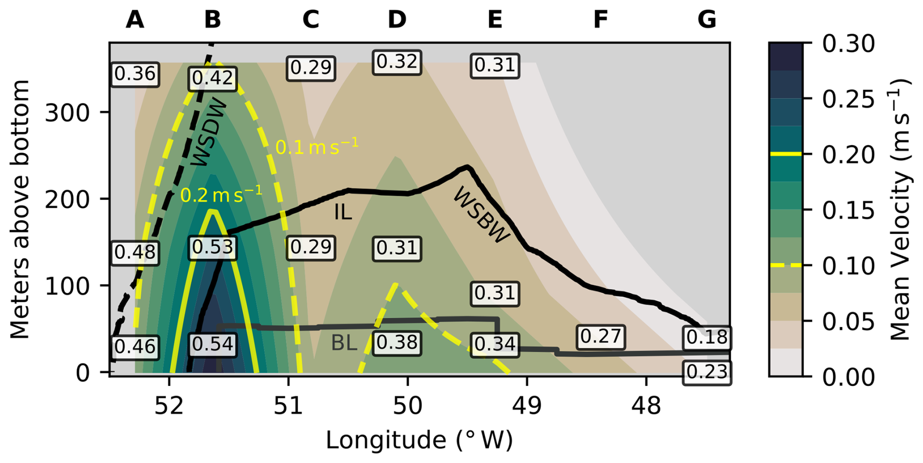
Figure 4 Mean flow field across the continental slope. Absolute velocities are time-averaged over the moored measurement period from January 2017 to January 2019 and linearly interpolated between measurement locations. Gray boxes show rotor current meter positions, labeled with the peak current speed during the measurement period in units of m s⁻¹. Moorings are labeled A–G. Black lines delineate water masses (WDW–WSDW, WSDW–WSBW) and gravity current layers (IL–BL).

The stratification of the lowermost 400 m varies along the transect. Shallower waters towards the shelf show more variability, with buoyancy frequency fluctuating around $\mathrm{1.1}\times {\mathrm{10}}^{-\mathrm{3}}$ rad s⁻¹. Further down the continental slope, stratification between 400 m and 200 m above the seafloor, above the gravity current, decreases to be almost constant at $\mathrm{0.3}\times {\mathrm{10}}^{-\mathrm{3}}$ rad s⁻¹. Inside the gravity current, stratification first increases up to a maximum, then decreases again closer to the seafloor, before dropping to almost zero directly above it, indicating a homogeneously mixed bottom boundary layer of around 10 m thickness (not shown).

We identify two regions inside the gravity current: a bottom layer (BL) and an interfacial layer (IL) above it. To quantify the extents of the two layers, we follow Fer et al. (2010) and define the BL height as the height at which the difference in neutral density to the bottommost value exceeds 0.01 kg m⁻³. The IL above is the region from the edge of the BL to the 20.40 kg m⁻³ isopycnal, which defines the upper boundary of the gravity current. The bottom layer varies between 20 and 60 m in height across the slope and decreases in thickness towards the deep sea (Fig. 4). A similar pattern of a decrease in height towards the deep sea is more strongly seen in the gravity current. We highlight a possibly confusing common nomenclature and point out that the gravity current bottom layer (BL) is not synonymous with a bottom boundary layer, which is usually thinner (Seim and Fer, 2011).

4.2 Turbulence patterns

Thorpe scale analysis reveals the across-slope pattern of turbulence (Fig. 5). Across the slope we see a quiescent region of the water column, above the gravity current, with dissipation rates ε_total of 10⁻⁹ W kg⁻¹ down to the background threshold of 10⁻¹⁰ W kg⁻¹. These quiescent areas extend into the Weddell Sea Bottom Water gravity current. At the interface of the IL layer with the Weddell Sea Deep Water, fewer and smaller overturns than in the BL are detected, which results in an ε_total estimation of around 10⁻⁹ W kg⁻¹, not noticeably different from the quiescent middle of the water column. In the BL, close to the seafloor, we measure enhanced dissipation rates ε_total around 10⁻⁸ W kg⁻¹. The binned data show these turbulent patches of bottom-enhanced turbulence extending beyond the BL, especially between 49.5 and 52° W. A closer look into individual profiles shows that while most overturns are detected inside the BL, some overturns across the layer boundary are identified (not shown). Their effect is emphasized in the averaging as dissipation rates follow a lognormal distribution, while densities from which the average BL are computed are approximately normally distributed. Our definition of the BL is independent of vertical density gradients and may not well represent the stratification of a singular profile.

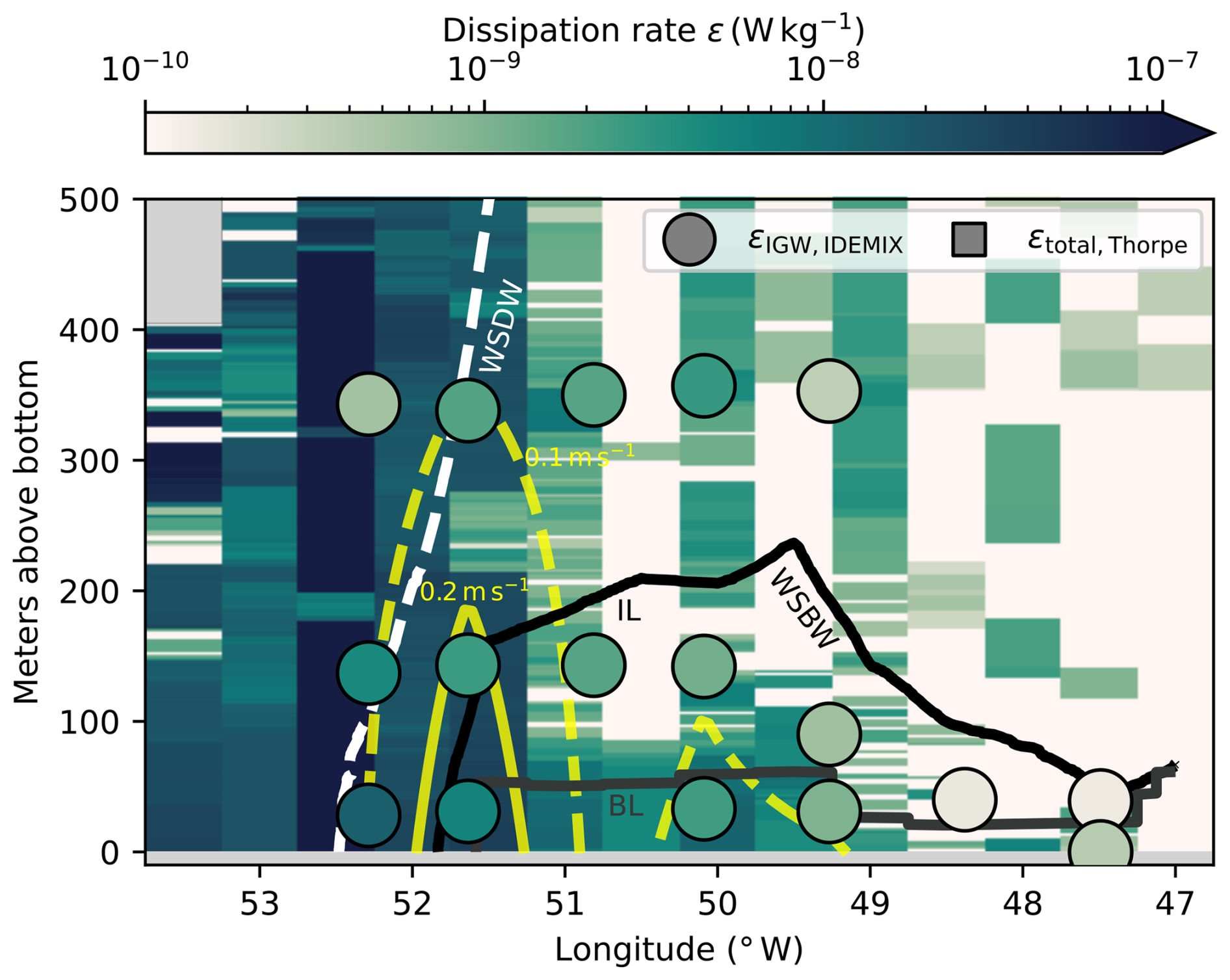
Figure 5 Dissipation rates in longitudinal bins across the continental slope. The background shows total dissipation rates ε_total,Thorpe from Thorpe scale analysis. Gray rectangles mark where no data are available because the height above the seafloor exceeds the total water column depth. Circles show wave-induced diffusivities ε_IGW,IDEMIX, calculated with Eq. (5) from velocity time series. Isolines of mean absolute velocity (yellow) show the gravity current cores. Boundaries of water masses (WDW–WSDW, WSDW–WSBW) and gravity current layers (IL–BL) are drawn as lines.

The transition of the IL to the BL is generally characterized by strong stratification and a sudden increase in dissipation rate. Similar gravity current structures of increased turbulence near the bottom and weak turbulence across an interface are found in the Baltic Sea (Umlauf et al., 2007), the Faroe Bank Channel (Fer et al., 2010; Seim and Fer, 2011), and Denmark Strait (Paka et al., 2013; North et al., 2018). Westward of 52° W, turbulence is elevated throughout the water column, with the highest turbulence observed at the shelf break, around 52.5° W (Fig. 5). This coincides with a strong horizontal gradient in the velocity flow field, caused by the Antarctic Slope Front (Thompson and Heywood, 2008, Fig. 9). Here, we observe total dissipation rates of up to $\mathrm{6}\times {\mathrm{10}}^{-\mathrm{7}}$ W kg⁻¹. At the westernmost edge of the gravity current, the two-layer description is not applicable, as the water column on the shelf becomes more homogeneously mixed.

We quantify dissipation rate induced by internal waves by using the two parameterizations described in Sect. 3.2 and 3.3. The results of Eq. (5), the parameterization based on wave energy, are shown as circles in Figs. 5 and 6. These calculated dissipation rates ε_IGW,IDEMIX range from 10⁻¹⁰ to 10⁻⁸ W kg⁻¹ and slightly decrease vertically with distance from the seafloor. This is observed at all mooring locations and is caused by the interaction of low stratification in the BL and vertical changes in wave energy. However, tidal wave energy has no clear dependence on height above the seafloor. For example, at mooring A the most energetic tides are measured closest to the seafloor and decrease in energy with height. At mooring B this pattern is reversed (Fig. B1). Along the transect, we observe a downslope decrease in ε_IGW,IDEMIX at all instrument levels. This results from weaker internal wave energy further away from the continental shelf. Additionally, we also see averaged over each mooring location a downslope decrease in the relative contribution of the semidiurnal baroclinic energy (not shown). This means the baroclinic tide decreases faster in energy than the internal wave continuum, which leads to it contributing relatively less energy to the overall wave energy available for turbulence.

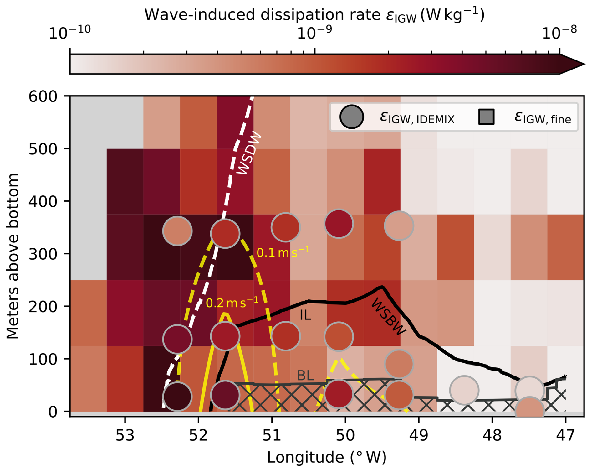
Figure 6 Comparison of the two independent methods for estimating internal-wave-induced dissipation rates ε_IGW. Fine-structure-based estimates (Sect. 3.3) are shown as rectangles in the background, while wave-energy-based estimates (Sect. 3.2) are shown as circles. Gray rectangles mark where no data are available, also because the height above the seafloor exceeds the total water column depth. Isolines of mean absolute velocity (yellow) show the gravity current cores. Boundaries of water masses (WDW–WSDW, WSDW–WSBW) and gravity current layers (IL–BL) are drawn as lines. The bottom layer (BL) is hatched to indicate that the methods possibly break down in the nearly homogenously mixed layer.

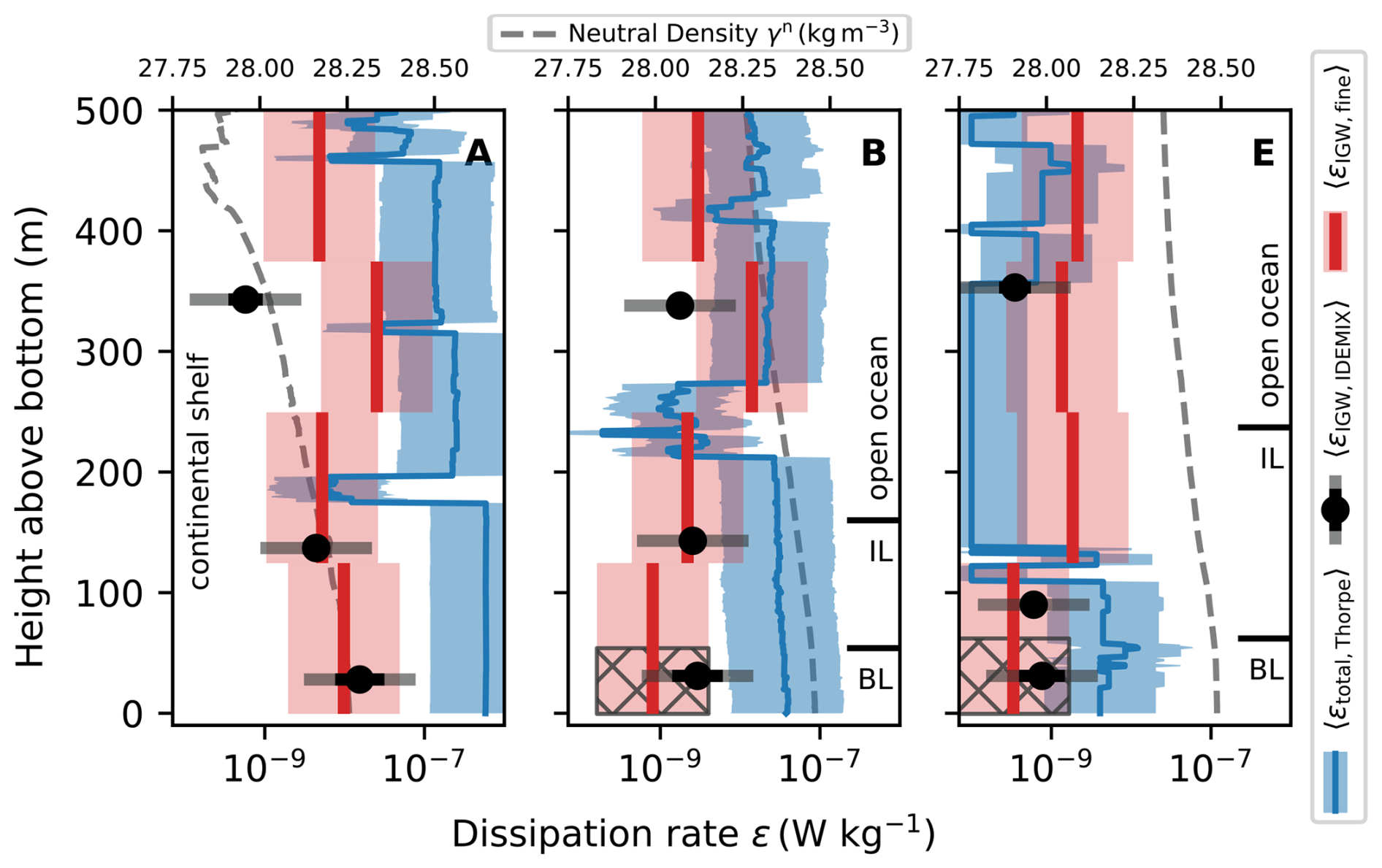
Figure 7 Exemplary dissipation rates around moorings A (52.2° W), B (51.6° W), and E (49.3° W). Profiles are taken from the longitudinal bins at 52.5, 51.5, and 49.5° W. The three panels show profiles of neutral density γⁿ, total ε_total,Thorpe, and wave-induced dissipation rates ε_IGW. For each method, the estimated uncertainty of a factor of 5 is plotted (Sect. 5.1). For the fixed-depth mooring-based ε_IGW,IDEMIX, the uncertainties are overlaid by the numerical errors of the method (Appendix C).

The results of the fine-structure method (Eq. 9) also show a downslope decrease in ε_IGW,fine over all heights above the seafloor. This is apparent in Fig. 6, with wave energy dissipation rates up to $\mathrm{2}\times {\mathrm{10}}^{-\mathrm{8}}$ W kg⁻¹ at the shelf break at 52.5° W and around $\mathrm{3}\times {\mathrm{10}}^{-\mathrm{10}}$ W kg⁻¹ or less in the deep sea. Compared to the horizontal pattern, vertical changes in ε_IGW,fine are small. Inside the interfacial layer of the gravity current, we see a downslope decrease in estimated dissipation rates ε_IGW,fine from $\mathrm{3}\times {\mathrm{10}}^{-\mathrm{9}}$ to $\mathrm{1}\times {\mathrm{10}}^{-\mathrm{10}}$ W kg⁻¹. Measurements outside the gravity current can be both more and less turbulent, with no apparent pattern. The resolution of the fine-structure method of 125 m exceeds the scale of the two-layer structure, and the individual layers cannot be resolved. As some assumptions underlying the fine-structure method break down in the almost completely mixed bottom layer, we hatch the bottom layer to mark the results as unreliable. The various assumptions of both the fine-structure parameterization and the wave energy parameterization as well as their validity will be discussed in Sect. 5.1.2.

Despite describing the same concept of wave-induced dissipation rates ε_IGW, the two presented methods differ in their exact results. This is an expected outcome because both methods estimate the dissipation rate from different larger-scale observables. Both methods for wave-induced dissipation rates agree on the horizontal pattern of high wave-induced turbulence towards the shelf and a more quiet water column towards the deep sea. In the direct comparison, 14 out of the 17 ε_IGW,IDEMIX estimations are within a factor of 5 of the nearest binned ε_IGW,fine result (not shown). A total of 11 data points are within a factor of 3. The biggest difference of about a factor of 15 is estimated at the westernmost mooring, mooring A, 320 m above the seafloor (see Fig. 6 and Fig. 7). We observe a possible depth dependence, as inside the gravity current the ε_IGW,IDEMIX estimates are higher, while further than 300 m from the seafloor, the fine-structure method results in higher bin-averaged values. This pattern is robust against comparing the ε_IGW,IDEMIX results to the fine-structure values from the second-closest longitudinal bin. Any functional relation between the two different methods remains inclusive, as statistics are limited by the number of rotor current meters.

Figure 7 shows the results of all methods on the continental shelf at mooring A, in the main core of the gravity current at mooring B, and towards the deeper parts of the gravity current at mooring E. Consistency demands that wave-induced dissipation rates ε_IGW are strictly lower than total dissipation rates ε_total, induced by all possible processes. This is observed over the whole transect; where ε_IGW exceptionally exceeds ε_total (for example at mooring E, Fig. 7), the differences remain below the uncertainty bounds. Larger differences between ε_total and ε_IGW occur in the more turbulent bottom layer (for example, at mooring B in Fig. 7). We remark that the averaging in each 0.5° longitudinal bin smooths out the shown density profiles. In individual profiles, sharper density gradients can occur.

4.3 Regional averages of dissipation rates

The observed horizontal and vertical patterns in stratification and turbulence show a two-layer structure inside the gravity current and a horizontal decrease in turbulence strength downslope. From this, we divide the transect into four regions: continental shelf, interfacial layer, bottom layer, and open ocean. The interfacial layer and the bottom layer are defined from neutral density (Sect. 4.1). The BL height is the height at which the difference in neutral density to the bottommost value exceeds 0.01 kg m⁻³. The IL above is the region from the edge of the BL to the 20.40 kg m⁻³ isopycnal, which defines the upper extent of the gravity current. We define the continental shelf region as everything west of 52° W, where no Weddell Sea Bottom Water is observed. This corresponds to depths shallower than 1000 m (Figs. 1c and 2). The open-ocean region is then the area above the gravity current, east of 52° W. But because the transect does not extend much beyond the continental slope (Fig. 1), our category of “open ocean” should not be mistaken with the inner Weddell Sea. We split the previously presented data into these regions, up to 600 m above the seafloor, and compute average total 〈ε_total,Thorpe〉 and wave-induced 〈ε_IGW,fine〉 turbulence in each region. We take the arithmetic mean of ε_total,Thorpe in each region directly, while the fine-structure results ε_IGW,fine are first nearest-neighbor-interpolated to a visually indistinguishable higher vertical resolution. This enables splitting of bins between regions. The parameterization based on wave energy from velocity time series does not have the necessary spatial resolution for regional averages.

Table 3 Region-averaged dissipation rates for the fine-structure and Thorpe scale method. The results of the fine-structure method in the BL are not reliable (Sect. 5.1.2) and given here in parentheses for the sake of transparency and completeness. The parameterization based on wave energy from velocity time series does not have the necessary resolution for meaningful averages in each region.

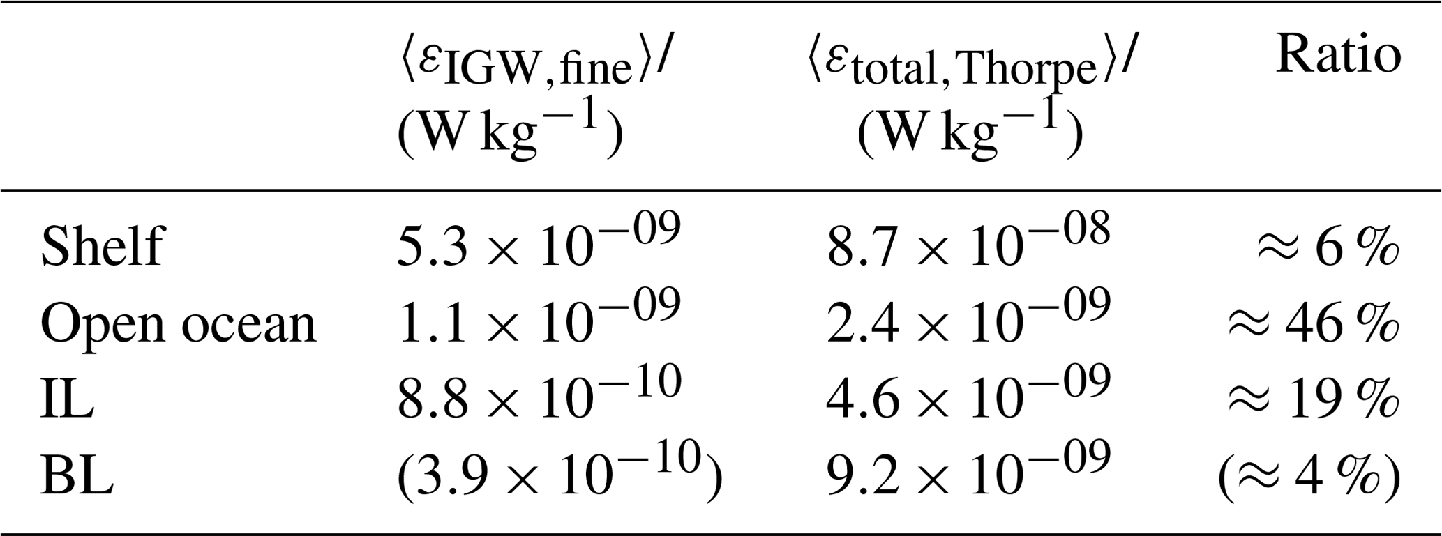
The highest averaged dissipation rate is observed on the shelf by both the Thorpe scale approach and fine-structure method (Table 3). The lower ratio of total and wave-induced turbulence suggests that internal waves play a smaller role for mixing on the shelf. The second-highest average total dissipation rate 〈ε_total,Thorpe〉 is measured in the bottom layer. The concept of wave-induced turbulence possibly loses its meaning inside the BL, as a homogenously mixed layer prevents the propagation of internal waves. Even though the result for wave-induced turbulence is not reliable, the large difference between 〈ε_total,Thorpe〉 and 〈ε_IGW,fine〉 supports the assumption that the bottom layer is largely mixed by processes other than internal wave breaking, like barotropic tides, convection, or friction between mean flow and seafloor.

Higher up, in the interfacial layer, region-averaged total and wave-induced dissipation rates are slightly closer in magnitude and differ by a factor of 5. Although the averaged dissipation rates in the open ocean do not considerably change from their respective values in the interfacial layer, we see closer agreement of Thorpe scale and fine-structure estimates. This is congruent with the assumption that away from the main forcing areas at the ocean's surface and bottom, turbulence is mainly caused by internal waves. From this order-of-magnitude perspective, we cannot exactly quantify the proportion of turbulence driven by internal waves in the gravity current. However, the ratios can be interpreted such that in the interfacial layer and the open ocean, internal waves are responsible for a sizable fraction of the turbulence.

5 Discussion

5.1 Dissipation rate uncertainties

For any meaningful comparisons between the computed dissipation rates, we have to include the error margins of each method. Direct microstructure measurements of dissipation rates, which could act as a benchmark, are not available along the Joinville transect. Therefore, we rely on an understanding of the scopes, numerical error calculations, and published uncertainty estimates of the methods. Any comparison of dissipation rates is necessarily a comparison over spatiotemporal scales due to the different types of measurements underlying the methods. Whalen (2021) showcases how different scales of averaging can introduce spurious discrepancies between a factor of 2 and a factor of 10, depending on the turbulence strength. By calculating averages over different years and 0.5° longitude bins, we try to take into account the inherent large variability of turbulence in time and space (Gregg et al., 1993; Moum et al., 1995).

While mooring time series provide year-round data, the seasonal distribution of ship-based CTD profiles is heavily biased towards the austral summer. To see whether the CTD profiles are representative of the long-term mean state, we calculate low-resolution profiles from temperature and salinity measurements from each mooring. Temperature and salinity time series measured at multiple depths on each of the seven moorings are first binned to daily averaged values and then linearly interpolated in the vertical to yield approximate segments of temperature and salinity. The long-time averages of the segments agree well with mean temperature and salinity profiles calculated from CTD profiles around each mooring. A difference in variability is not observed, as the CTD profiles cover the complete range of values observed by the moored instruments (not shown). Therefore, we can use the CTD profiles to describe the long-term-averaged hydrographic state.

5.1.1 Uncertainties of total dissipation rates

For the proportionality constant between the Thorpe and Ozmidov scale, we use a tested literature value of 0.8, but there is evidence that the correlation is not necessarily constant (Mater et al., 2015; Mashayek et al., 2017). Although we follow standard oceanographic practice, results like those of Scotti (2015) show that the usual practice may only hold for turbulence from shear-driven flows. They find that, when turbulence is instead driven by the available potential energy of the mean flow (also called convection-driven), the proportionality factor between the Thorpe scale and Ozmidov scale is no longer 𝒪(1). Gravity currents are ultimately driven by their available potential energy, but we expect both convection and shear instabilities to occur due to a nonuniform flow field and breaking internal waves. Without any further knowledge about the underlying processes, the standard practice is our best estimate of process-independent dissipation rates.

In the calculation of ε_total,Thorpe (Eq. 1) small overturns and measurement noise are undistinguishable and are cut off to not include spurious turbulence, controlled by the density noise parameter. This can lead to a bias against quiescent regions, in which the dissipation rate is determined with higher uncertainties. We investigate Thorpe scale estimates across the transect by fitting a lognormal distribution to the corresponding histogram (not shown). Although Thorpe scales of few centimeters are physically possible (Johnson and Garrett, 2004), we expect these missing small scales to only contribute little to the overall turbulence pattern, as we resolve the large majority of the theoretically predicted Thorpe scales. To see if our application of the Thorpe scale method is limited by the depth resolution or the density resolution, we employ a test for the relative importance, suggested in Stansfield et al. (2001). The parameter

$$\begin{array}{}\text{(13)}& R={\displaystyle \frac{\mathrm{d}{\mathit{\gamma }}^{\mathrm{n}}}{\mathrm{d}z}}{\displaystyle \frac{\mathrm{\Delta }z}{\mathrm{\Delta }{\mathit{\gamma }}_{\mathrm{instr}}^{\mathrm{n}}}}={\displaystyle \frac{\mathrm{d}{\mathit{\gamma }}^{\mathrm{n}}}{\mathrm{d}z}}{\displaystyle \frac{\mathrm{1}\mathrm{m}}{\mathrm{1}\times {\mathrm{10}}^{-\mathrm{3}}\mathrm{kg}{\mathrm{m}}^{-\mathrm{3}}}}\end{array}$$

relates a smooth background density gradient to the ratio of depth and density resolution of the CTD instrument. If R>1, depth resolution is the limiting factor, whereas if R<1 it is the density resolution limiting our results. We fit to each exemplary neutral density profile (Fig. 7) a cubic background and insert the instrument resolution values from Sect. 2. Across all tested profiles, R stays below a value of 1, confirming density resolution to be the limiting factor (not shown).

The almost homogenously mixed BL is a recurring problem in all methods of turbulence quantification used here. Though the BL is defined to have no density differences greater than 0.01 kg m⁻³, we are able to detect differences 1 order of magnitude smaller (Sect. 2) and therefore possible overturns inside the bottom layer. This means the Thorpe scale approach allows accurate dissipation rate estimates in the BL, within the limits of its uncertainties. The Thorpe scale method is estimated to be generally within a factor of about 5 of direct microstructure measurements (Dillon, 1982; Ferron et al., 1998; Alford et al., 2006). Although microstructure measurements have their own associated uncertainties, we take the factor of 5 as an uncertainty of the Thorpe scale method itself.

5.1.2 Uncertainties of wave-induced dissipation rates

Both parameterizations of wave-induced dissipation rates assume (a) that a stratification exists (N²>0) for internal gravity waves (IGWs) to propagate and (b) that all observed variability on the considered scales is associated with internal gravity waves. The bottom layer is defined as having almost zero stratification, and the fine-structure parameterization is consequently not applicable here. However, we observe a maximum height of the BL of around 60 m, which is much smaller than the length of 187 m of the lowest vertical segment in the fine-structure parameterization. Therefore, the BL may affect the results of the bottommost bins but does not invalidate them. To visualize this limitation, we hatch the BL in Figs. 6, 7, and D1. While the fine-structure method cannot be accurately applied in the BL, we still present its results here, as the ratio to the total dissipation rate informs us about the locally dominating physical processes. Figure 6 shows that the bottommost velocity recorders at moorings B, D, and E are located inside the BL. Across all rotor current meter locations, the average stratification N ranges from $\mathrm{6.1}\times {\mathrm{10}}^{-\mathrm{4}}$ to $\mathrm{2.1}\times {\mathrm{10}}^{-\mathrm{3}}$ rad s⁻¹ (see Sect. 3.2.3), greater than the minimum required stratification of $N_{\min }=\mathrm{4.5}\times {\mathrm{10}}^{-\mathrm{4}}$ rad s⁻¹ described in Kunze et al. (2006, Sect. 4) for the fine-structure method. Therefore, the computation of wave-induced dissipation rate estimates ε_IGW,IDEMIX from moored velocity time series (Sect. 3.2) is applicable in the BL. We hypothesize that averaged over longer time spans, the weak stratification allows for internal waves, while each fine-structure profile represents a singular point in time at which internal waves may not be able to propagate. An observation of this behavior in the Red Sea outflow plume is described in Peters and Johns (2006). The problem of a potentially homogenously mixed BL is therefore less prevalent in the ε_IGW,IDEMIX parameterization based on wave energy, as long as the calculated average buoyancy frequencies are large enough to be acceptable.

While a stratification exists in the interfacial layer (IL), the second assumption could still not hold. Due to the possible prevalence of variability on IGW scales caused by non-IGW processes, Seim and Fer (2011) generally dismiss the use of a parameterization of dissipation rates from wave energy in the interfacial layer of gravity currents. We consider in the integration for strain variance in the fine structure (Eq. 8) only the resolved length scales associated with waves. How much of that spectral range is “contaminated” by non-wave processes is impossible to determine here. All measured energy spectra resemble the smooth spectral decay associated with an internal wave continuum (see, for example, the spectrum in Fig. 3b). When we apply both methods for wave-induced dissipation rates, our results are of similar magnitudes and physically plausible, as estimated ε_IGW values are on average less than estimates of ε_total. We see a careful use of the two parameterizations in the IL as justified, as long as the caveats are explicitly described.

Although the basis of the wave energy method (see Sect. 3.2) is also used in the fine-structure parameterization, to the knowledge of the authors, our particular approach of calculating the wave-induced dissipation rate from velocity time series has not been applied in prior studies and comparisons with direct microstructure measurements are not available. From the variability of the N² profiles and uncertainties in the wave energy calculation, we estimate for the wave energy method numerical uncertainty of an average factor of around 1.5 up to a factor of 2.3 (see Appendix C for the calculation). However, this approach only accounts for errors introduced by the method calculations themselves. For example, the numerical uncertainty of ε_IGW,IDEMIX is generally larger close to the seafloor, where N is most variable (Fig. 7). Due to the parameterization from wave energy having the same underlying theory as the fine-structure method, we would expect a similar general uncertainty of a factor of 5.

For the error of the strain-based parameterization with R_ω=7 in the Arctic Ocean, Baumann et al. (2023) find that 73 % of the estimates are within a factor of 5 of microstructure observations. This is in agreement with global estimates from Polzin et al. (2014), finding uncertainty “substantially less” than a factor of 10, while Whalen et al. (2015) estimate global agreement between micro-structure and fine structure mostly within a factor of 2 to 3. Together with the following specific biases, we follow the more conservative estimate and use an uncertainty factor of 5 for the fine-structure method. The results of the fine-structure parameterization are influenced by several parameter choices. One example involves the integration limits in the variance calculation (see also the discussion in the appendix of Pollmann, 2020). We choose a hybrid approach of confining the upper integration limit m_c with both a fixed minimum length scale and a maximum canonical variance. Dynamically adjusting this cut-off wave number for the integral to not exceed a maximum variance is a common approach (Gregg et al., 2003; Kunze et al., 2006; Seim and Fer, 2011; Pollmann et al., 2017), but the chosen value varies between studies. Other possibilities to determine integration limits are to set them to fixed values (Fine et al., 2021), to manually check measurement noise levels (Baumann et al., 2023), or to relate the limits to stratification via a maximum Richardson number (Meyer et al., 2015; Pollmann, 2020). Similarly, the wave number chosen for the lower integration limit m₀ varies across applications of the fine-structure parameterization, depending on vertical segment lengths and relevant wave scales.

We determine the local shear-to-strain variance ratio R_ω from a subset of 18 hydrographic profile data points on the 2022 PS129 cruise, where shear measurements are available, and take the observed value of R_ω=7.9 as validation for the literature value of R_ω=7. With this correction, the two formulations of the fine-structure method, dependent on strain (Eq. 9) and on shear (see Appendix D), differ in almost all segments by a factor less than 5 (see Fig. D1). This comparison possibly indicates a slight overestimation of wave-induced turbulence inside the gravity current, as the ratio shows a cross-slope dependence, with the lowest strain-to-shear ratios reached in the deep open ocean. Another indication for a possible overestimation is given by Waterman et al. (2014), who observe overprediction by the fine-structure method near topography in the Antarctic Circumpolar Current. They attribute this bias of a factor of 5, compared to microstructure estimations, to not yet understood non-wave mixing processes in the Southern Ocean. This overprediction is observed acting on a vertical scale from the bottom to 1500 m above the seafloor, far larger than what we consider here. By comparing ε_IGW,fine to process-blind turbulence estimates ε_total,Thorpe, we see that the fine-structure results are consistently lower than the total dissipation rate and therefore physically plausible. Nonetheless, the overprediction described by Waterman et al. (2014) could be a systematic error.

The large uncertainties in the dissipation rate estimates lead us to refrain from calculating turbulent diffusivities. Especially the uncertainty of buoyancy frequency N at the locations of the time series measurements, as well as the extensive discussions surrounding the mixing parameter Γ (Gregg et al., 2018, and references therein), would only increase the uncertainty of the results without leading to new insights.

5.2 Wave sources inside and outside the f–N frequency range

Predominantly, internal waves are generated by fluctuating wind stress at the sea surface and flow–topography interaction (e.g., Musgrave et al., 2022). The latter can occur through oscillating flows (the tides), leading to internal waves of tidal frequency, and non-oscillating flows (e.g., mean flow, mesoscale eddies), leading to lee waves. Both strong diurnal and semidiurnal tides (Foldvik et al., 1990; Robertson, 2001a, b) are present in the Weddell Sea (Fig. 3b), and the multiple ridges (Dorschel et al., 2022) and slopes in the vicinity of the transect (Fig. 1c) might be relevant generation sites of both internal tides and lee waves. Exact generation estimates unfortunately cannot be provided here because state-of-the-art datasets are masked in much of the Weddell Sea: sediment cover precludes the estimation of the lee wave generation at small-scale abyssal hills (e.g., Eden et al., 2021), numerical model simulations do not resolve the high-latitudes sufficiently well (Buijsman et al., 2020), and steep continental slopes render the typically applied linear theory for internal tide generation invalid (e.g., Pollmann and Nycander, 2023). Linear wave kinematics also form the backbone of wave-induced dissipation rate estimates (Eqs. 5 and 9) exploited here. The internal waves they describe can propagate freely as long as their frequency remains between the local Coriolis frequency f and the buoyancy frequency N. In particular, the energetic low modes can propagate over large distances from their generation sites (Zhao et al., 2016; Alford et al., 2019), which implies that the wave energy we observe in our study region can have both local and nonlocal contributions. The critical latitude for free propagation (f=ω) is near 30° for the diurnal and near 75°for the semidiurnal internal tides (Robertson et al., 2017, Table 1). Poleward of the critical latitude, the linear solution to the wave equation is exponentially decaying such that the internal waves generated from tide–topography interaction become bottom-trapped (Falahat and Nycander, 2015). Moreover, the nonlinear solution begins to be relatively more important: Rippeth et al. (2017) show in a proof-of-concept modeling study combined with observations from the Arctic Ocean that under certain conditions nonlinear tide-generated internal waves can notably enhance the local mixing and can also propagate away from their generation site. In global-scale analyses of wave-driven mixing and in parameterizations thereof (e.g., de Lavergne et al., 2019; Brüggemann et al., 2024), the bottom-trapped and nonlinear internal tide generation is typically neglected because the linear solution is by far the dominant contributor (Falahat et al., 2014; Falahat and Nycander, 2015). Since the Joinville transect is located at 64° S – that is, equatorward of the critical latitude for the most energetic semidiurnal M2 tide – we are confident that we can follow this line of reasoning here and expect the error from neglecting the bottom-trapped and nonlinear contributions to be small.

5.3 Requirements for model comparisons

We compare our results to a static global map of tide-driven dissipation rates (de Lavergne et al., 2020). The authors combine the effects of low modes (mode number 1–10), attenuation by wave–wave interactions, direct breaking of low-mode waves through shoaling, low-mode waves dissipating at critical slopes, scattering of low-mode waves by abyssal hills, and generation of high-mode waves by abyssal hills to derive their dataset (de Lavergne, 2020). Along the Joinville transect, the authors obtain tidally induced dissipation rates down to 10⁻¹¹ W kg⁻¹, below the sensitivity threshold of usual turbulence measurements (not shown). In contrast, our wave-induced dissipation rate estimates (Fig. 6) are significantly higher, particularly toward the shelf. However, a direct comparison between their mixing scheme and our results is difficult, as internal tides lose energy to the continuum through wave–wave interactions and cannot be cleanly isolated in observations from internal waves of other frequencies.

Rather than comparing our results to a static dissipation map, we could consider the output of numerical ocean models, which explicitly include the contribution of internal waves to mixing. However, global models of this kind (e.g., Brüggemann et al., 2024) lack the resolution needed to capture the gravity current. Bottom water formation at high latitudes is heavily parameterized in modern climate models to address biases in deepwater formation (Heuzé, 2021). For a meaningful comparison, a model would need to differentiate between wave and non-wave turbulence-driving processes while directly simulating the Weddell Sea Bottom Water gravity current. To our knowledge, no existing model run meets these criteria. Current simulations are either too coarse or, at smaller scales, differ too much from observations in terms of the gravity current's size, stratification, or physical properties.

5.4 Turbulence strength and drivers in comparable gravity currents

At Cape Darnley, another formation site of Antarctic Bottom water, Hirano et al. (2015) observe dissipation rates of $\mathit{\epsilon }>{\mathrm{10}}^{-\mathrm{7}}$ W kg⁻¹ in a 10 m thick bottom boundary layer of a gravity current using turbulence microstructure profilers. As tidal currents at Cape Darnley are limited to small amplitudes, they attribute the main energy source of turbulence to the gravity current itself. In their study of the Faroe Bank Channel overflow, Seim and Fer (2011) calculate horizontal kinetic energy in the gravity current from velocity spectra and use the fine-structure method to obtain dissipation rates in the ambient above. Without calculating wave-induced dissipation rates in the gravity current, they conclude that “internal wave‐induced mixing in IL can be significant and should not be ignored”. In contrast, North et al. (2018) associate in their study of the Denmark Strait overflow high dissipation rates in the IL with shear instabilities, as they observe high shear and Richardson numbers below the critical value of 0.25. Their observations and conclusions differ from ours, as the Denmark Strait overflow displays much higher current velocities up to 1 m s⁻¹, causing high shear (North et al., 2018, Fig. 2). In comparison, the Weddell Sea Bottom Water gravity current has in its cores mean flow speeds of about 0.3 m s⁻¹ and peak velocities of 0.54 m s⁻¹ (see Fig. 4 and also Llanillo et al., 2023, Figs. 7 and 8). Therefore, we expect shear instabilities to play less of a role at our study site. Schaffer et al. (2016) present another mechanism for turbulence production, sourced by flow–topography interaction in the Denmark Strait overflow. They observe locally elevated turbulence upstream of small topographic elevations, less than 2 km wide and 80 m tall (Schaffer et al., 2016, Fig. 11), and explain it with a mechanism described in Legg (2014): low-mode internal waves interact with isolated topography and propagate upstream, where they get arrested, break, and cause turbulence. Due to the strong internal wave field we observe, this process could also happen in the Weddell Sea Bottom Water gravity current. However, lacking measurements of along-slope instead of across-slope turbulence patterns, we cannot determine the relevance of this mechanism at our study site.

5.5 Turbulence along the Weddell Sea Bottom Water gravity current

We want to put our results in a greater context by comparing them to other dissipation rate measurements along the Weddell Sea Bottom Water gravity current. Upstream of the mooring array, in the southern Weddell Sea close to the Filchner–Ronne ice shelf, Fer et al. (2016) observe a bottom layer of 100 m thickness, in which they measure dissipation rates of up to 10⁻⁷ W kg⁻¹ using a microstructure profiler. Because this site lies south of the M2 critical latitude, Fer et al. (2016) conclude that trapped waves generated on the upper continental slope cause strong turbulence. Due to the vicinity of the semidiurnal critical latitude, the semidiurnal internal tide is bottom-trapped and dissipates its energy in the bottom boundary layer. In comparison, further downstream of the Weddell Sea gravity current towards the Scotia Sea around the Orkney Plateau, Naveira Garabato et al. (2019) observe dissipation rates of 10⁻⁹ to 10⁻⁷ W kg⁻¹ over the slope in the bottom 250 m, which they attribute to symmetric instabilities. At this point, the gravity current core has already descended to depths below 3000 m, which approximately corresponds to measurements east of 50° W at our study site on the Joinville transect. At these depths, we see a significant decrease in wave-induced dissipation, indicating a different dominant mixing process.

The comparison with other dissipation rate estimates in gravity currents suggests that dominant mixing processes are strongly location-dependent. We suspect that for wave-induced turbulence to dominate, the gravity current must pass a “Goldilocks zone”, neither too deep nor too shallow on a sloping topography, where the internal wave field is most energetic. In this environment, the highest dissipation rates are still found in the bottom layer, driven by non-wave processes. However, this layer is largely isolated from overlying ambient water, and mixing therein cannot lead to increased entrainment. Instead, we show that in this situation, internal waves are responsible for a large fraction of the total dissipation rate in the gravity current interfacial layer and its boundary to ambient water.

To embed our results in the larger discussions of a changing climate, we point to results from Strass et al. (2020), who demonstrate persistent warming of the interior Weddell Sea. Furthermore, they hypothesize that advection-driven temperature rises in Warm Deep Water or Weddell Sea Deep Water could result in enhanced heat transfer into Weddell Sea Bottom Water by entrainment into the gravity current. Zhou et al. (2023) show a 30 % volume decrease in Weddell Sea Bottom Water since 1992, most pronounced in the densest water classes. Although they attribute this decrease to large-scale changes in the Weddell Gyre like multidecadal wind patterns, we hypothesize a possible positive feedback loop: as the density differences between the gravity current and the surrounding water become smaller, stratification decreases, which enables more efficient vertical mixing. This would lead to increased entrainment of lighter water and consequentially accelerated density loss in the Weddell Sea Bottom Water. These changes to Antarctic Bottom Water export could have far-reaching consequences for the stability of the global current system.

6 Conclusions

The potentially crucial role of internal waves as turbulence drivers within gravity currents has been hypothesized or inferred in previous studies but rarely quantified. Here, we present an approach to estimate wave-induced dissipation rates in a gravity current using standard oceanographic data. Combining moored and shipboard observations, we derive statistical estimates of dissipation rates in the Weddell Sea Bottom Water gravity current. Our study introduces a novel application of a parameterization that computes wave-induced dissipation rates from wave energy, calculated from moored velocity time series. The resulting estimates agree reasonably well with those from the established fine-structure analysis method, differing in 1 out of 17 data points by less than a factor of 3. Further statistical comparisons are limited by the number of moored velocity time series.

We find that internal-wave-induced dissipation rates are approximately 2 orders of magnitude higher in the shallow region near the Antarctic continent than in the deep ocean. Dissipation rate estimates from Thorpe scales reveal that, although bottom processes cause the highest amount of turbulence in the gravity current, the top of the interfacial layer is at a far enough distance to be largely unaffected by these. Instead, internal waves are responsible for a large fraction of the total dissipation rates within this layer and therefore for entrainment of ambient waters into the gravity current. The exact quantification of the effect of internal tides on turbulence in the gravity current is complicated by large uncertainties in the dissipation rate estimates, but the general spatial patterns are clear.

The large scale of the Weddell Sea Bottom Water gravity current makes it a key player in global overturning circulation but hinders observing its dynamics at high resolution. Our description of spatial distribution and drivers of turbulence contributes to a better understanding of the gravity current and its features. Identifying temporal changes in dissipation rates across the continental slope, in terms both of trends and interannual and seasonal variability, is part of our ongoing work.

Our conclusion of wave-induced turbulence as an important contributor to turbulence along the Joinville transect cannot simply be transferred to other gravity currents. Comparison with the scientific literature shows that the dominant mixing processes are heavily dependent on the environment. In our case, multiple conditions like height and location of the gravity current on a sloping topography in an area with strong tides combine to facilitate the importance of internal waves.

Appendix A: Relation of horizontal kinetic to total wave energy

To calculate total wave energy from velocity observations, the contribution of potential energy must be taken from wave theory. For linear internal waves in the frequency range between f and N, the relation between horizontal kinetic energy spectra 𝒰 and total energy spectra ℰ is known (Olbers, 1983; Olbers et al., 2012, Sect. 7.2.2; Pollmann, 2017, Sect. 5.2, and references therein). Because our velocity measurements contain internal waves of all wave numbers, we denote horizontal kinetic energy spectra 𝒰(z,ω) only as a function of wave frequency ω and depth z:

$$\begin{array}{}\text{(A1)}& \begin{array}{rl}\mathcal{U}(z,\mathit{\omega })& =\int {\displaystyle \frac{\mathrm{1}}{\mathrm{2}}}{\displaystyle \frac{N(z{)}^{\mathrm{2}}-{\mathit{\omega }}^{\mathrm{2}}}{N(z{)}^{\mathrm{2}}-f^{\mathrm{2}}}}{\displaystyle \frac{{\mathit{\omega }}^{\mathrm{2}}+f^{\mathrm{2}}}{{\mathit{\omega }}^{\mathrm{2}}}}\mathcal{E}(z,m,\mathit{\omega })\mathrm{d}m\\ & ={\displaystyle \frac{\mathrm{1}}{\mathrm{2}}}{\displaystyle \frac{N(z{)}^{\mathrm{2}}-{\mathit{\omega }}^{\mathrm{2}}}{N(z{)}^{\mathrm{2}}-f^{\mathrm{2}}}}{\displaystyle \frac{{\mathit{\omega }}^{\mathrm{2}}+f^{\mathrm{2}}}{{\mathit{\omega }}^{\mathrm{2}}}}\mathcal{E}(z,\mathit{\omega })\int A\left(m\right)\mathrm{d}m,\end{array}\end{array}$$

with wave frequency ω, buoyancy frequency N, and Coriolis frequency f, all in units of rad s⁻¹. We assume that we can factor out the wave number m dependency of the spectrum of total energy $\mathcal{E}(z,m,\mathit{\omega })=\mathcal{E}(z,\mathit{\omega })A\left(m\right)$. The same approach of factorization is used in the Garrett–Munk model (Munk, 1981), but in contrast, we are not required to make any further assumptions about the form of $\mathcal{E}(z,m,\mathit{\omega })$. As $\int A\left(m\right)\mathrm{d}m=\mathrm{1}$ (Pollmann, 2020, Eqs. 1–3), we can rearrange to Eq. (3) from the main text:

$$\begin{array}{}\text{(A2)}& \mathcal{E}(z,\mathit{\omega })=\mathrm{2}{\displaystyle \frac{N(z{)}^{\mathrm{2}}-f^{\mathrm{2}}}{N(z{)}^{\mathrm{2}}-{\mathit{\omega }}^{\mathrm{2}}}}{\displaystyle \frac{{\mathit{\omega }}^{\mathrm{2}}}{{\mathit{\omega }}^{\mathrm{2}}+f^{\mathrm{2}}}}\mathcal{U}(z,\mathit{\omega }).\end{array}$$

The presented proportionality factor between ℰ and 𝒰 diverges in the limit of ω→N. In comparison, the ratio of total to kinetic wave energy in the Garrett–Munk model approaches 2 in the limit of ω→N, meaning kinetic energy and potential energy contribute equally. In the limit of ω→f, total wave energy in both frameworks is fully captured by kinetic energy. In our analysis, we decide to use Eq. (A2), but for all resolved frequencies in our measured spectra, the difference to the Garrett–Munk model conversion factor is negligible.

Appendix B: Estimating baroclinic tidal energy

As one step to calculate total wave energy available for local dissipation from moored velocity records, we must separate the energy contained in internal baroclinic tidal waves from the depth-independent barotropic tide. To overcome the limitations of the low vertical resolution of the moorings, we run the Circum-Antarctic Tidal Simulation (CATS) model (Padman et al., 2002; Howard et al., 2019) using Tide Model Driver (Greene et al., 2024) for the duration of the moored velocity measurements. This regional inverse model simulates barotropic tidal horizontal velocities of the strongest constituents in the Southern Ocean (M2, S2, N2, K2, K1, O1, P1, Q1, Mf, and Mm) on a 4 km grid. As with measured velocities in Sect. 3.2, we calculate horizontal kinetic energy spectra and integrate over an interval around the semidiurnal frequencies. This predicts barotropic tidal energies for each mooring location. The modeled strength of the barotropic tide decreases exponentially from the shelf to the deep sea (Fig. B1). However, especially towards the shelf, the predicted energy at some depths exceeds the measured tidal energy at semidiurnal frequencies. We believe that this disagreement between model and measurements cannot be prevented by the use of a different tidal model. In their comparison of Antarctic Ocean tidal models, Sun et al. (2022, Fig. 4) conclude that at our study site of the Joinville transect in the northwestern Weddell Sea, any differences in the dominant M2 constituent between CATS and comparable models are small.

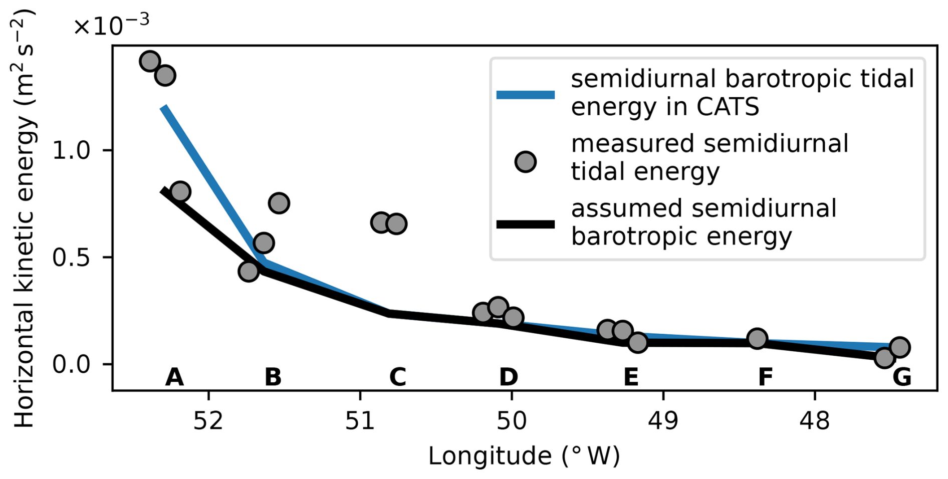
Figure B1 Comparison of predicted barotropic kinetic energy by the CATS model, measured semidiurnal tidal energies, and assumed best estimate for barotropic horizontal kinetic energy across the continental slope. Measured energies are shifted along the longitude axis for visualization purposes, where for each mooring the measurement closest to the seafloor is to the left. All moorings are labeled A–G, according to Table 2.

In cases where measured tidal kinetic energy is lower than barotropic tidal energy predicted by the CATS model (Fig. B1), the model prediction is discarded and instead we exploit the depth dependence of the baroclinic tide. We then take the lowest measured kinetic energy at semidiurnal frequencies at each mooring location as a new best estimate of the barotropic tide. The result shows a similar exponential decline, strongest on the shelf and weakest in the deep sea. Subtracting the barotropic energy from the measured tidal energies yields baroclinic horizontal kinetic energies. Tidal energy vertical variability can be seen in each group of points in Fig. B1, in which each energy measurement is shifted in longitude according to their distance from the seafloor. We sometimes observed the highest energy farthest from the bottom (moorings A, C, and E) and sometimes closest to the ground (moorings B and G). We hypothesize that the variable pattern is caused by spatial variations in the baroclinic tidal wave field. Finally, applying the scaling from Eq. (3) converts the baroclinic horizontal kinetic wave energies to baroclinic total wave energies, which we then use further in Sect. 3.2.4.

Appendix C: Wave energy parameterization error estimate

This section estimates the numerical error of the wave energy parameterization without accounting for the errors introduced by the many assumptions necessary for this dissipation rate parameterization from observations of larger scales. Repeating Eq. (5) in the main text,

$$\begin{array}{}\text{(C1)}& {\mathit{\epsilon }}_{\mathrm{IGW},\mathrm{IDEMIX}}(E,N)={\displaystyle \frac{\mathrm{1}}{\mathrm{1}+\mathrm{\Gamma }}}{\mathit{\mu }}_{\mathrm{0}}\left|f\right|\mathrm{arccosh}{\displaystyle \frac{N}{\left|f\right|}}{\displaystyle \frac{m_{*}^{\mathrm{2}}{E}^{\mathrm{2}}}{N^{\mathrm{2}}}},\end{array}$$

we want to calculate the uncertainty in our dissipation rate estimates. But from fine-structure results in this study and the general literature (Whalen, 2021), we know ε is approximately lognormally distributed. A symmetric additive error would therefore be nonsensical. Therefore, we calculate instead the error to the order of magnitude, computed as the common logarithm log ₁₀ of the dissipation rate, to achieve a multiplicative error, which is symmetric in log scale. We constrain ourselves here to only account for the largest errors introduced by the uncertainties in buoyancy frequency N and wave energy E and neglect uncertainties of the constants Γ, μ₀, f, and m_*. The method uncertainty $\mathrm{\Delta }{\log }_{\mathrm{10}}{\mathit{\epsilon }}_{\mathrm{IGW},\mathrm{IDEMIX}}(E,N)$ is then calculated with the ansatz of Gaussian error propagation as

$$\begin{array}{}\text{(C2)}& \begin{array}{rl}{\left(\mathrm{\Delta }{\log }_{\mathrm{10}}{\mathit{\epsilon }}_{\mathrm{IGW}}(E,N)\right)}^{\mathrm{2}}& ={\left(\mathrm{\Delta }N{\displaystyle \frac{\partial }{\partial N}}{\log }_{\mathrm{10}}{\mathit{\epsilon }}_{\mathrm{IGW}}(E,N)\right)}^{\mathrm{2}}\\ & +{\left(\mathrm{\Delta }E{\displaystyle \frac{\partial }{\partial E}}{\log }_{\mathrm{10}}{\mathit{\epsilon }}_{\mathrm{IGW}}(E,N)\right)}^{\mathrm{2}}\\ & =\left({\displaystyle \frac{\mathrm{\Delta }N}{\sqrt{N^{\mathrm{2}}-f^{\mathrm{2}}}\ln \left(\mathrm{10}\right)\arctan \left(\frac{N}{\left|f\right|}\right)}}\right.\\ & {\left.-{\displaystyle \frac{\mathrm{2}\mathrm{\Delta }N}{N\ln \left(\mathrm{10}\right)}}\right)}^{\mathrm{2}}+{\left({\displaystyle \frac{\mathrm{2}\mathrm{\Delta }E}{E\ln \left(\mathrm{10}\right)}}\right)}^{\mathrm{2}}.\end{array}\end{array}$$

All derivations and simplifications are calculated with the symbolic math library SymPy (Meurer et al., 2017).

However, determining the uncertainties ΔN of the buoyancy frequency and ΔE of the energy level is nontrivial. We take the uncertainty in N from N² variability. Instead of averaging N² profiles ΔN² at each mooring location to yield mean stratification profiles (see Sect. 3.2.3), we propagate their standard deviation ΔN² as a Gaussian error to the corresponding uncertainty:

$$\mathrm{\Delta }N={\displaystyle \frac{\mathrm{1}}{\mathrm{2}}}{\left(N^{\mathrm{2}}\right)}^{-\frac{\mathrm{1}}{\mathrm{2}}}\mathrm{\Delta }{N}^{\mathrm{2}}.$$

The calculation from squared buoyancy frequency N(z)² is done to allow averaging over small unstable stratified regions, in which N(z) would be imaginary. We motivate the shift from a natural variability of N² to an uncertainty in N to account for the error from assuming a constant-in-time buoyancy frequency profile.

Technically, ΔE is not independent of ΔN, as the buoyancy frequency determines the upper integration boundary of the spectrum in Eq. (4). However, Fig. 3b shows that energy density drops by about 2 orders of magnitude from f to N, while N only varies by 1 order of magnitude. Therefore, we assume independence of ΔE and ΔN in Eq. (C2). We determine wave energy error ΔE from the uncertainty of the slope extension, given by the fit algorithm itself. The upper and lower range of slope plus uncertainty is converted by integration of ℰ(ω) to an upper and lower range of total wave energy, yielding ΔE. This approach may slightly underestimate the uncertainty ΔE, as the error in the calculation of the rotary spectra (see Sect. 3.2) is neglected. The combined multiplicative uncertainty for the dissipation rate, determined from Eq. (C1) and averaged over all measurement locations, is around 1.5 up to a factor of 1.9. Some results of the uncertainty calculations are displayed in Fig. 7 and discussed in Sect. 5.1.2.

Appendix D: Shear-based formulation of the fine-structure parameterization

If stratification and shear profiles are measured, the fine-structure parameterization can be formulated as follows (Kunze et al., 2006) to calculate the wave-induced dissipation rate inside a segment (in the notation of Fine et al., 2021):

$$\begin{array}{}\text{(D1)}& {\mathit{\epsilon }}_{\mathrm{IGW},\mathrm{fine}}={\mathit{\epsilon }}_{\mathrm{0}}{\displaystyle \frac{\stackrel{\mathrm{‾}}{N^{\mathrm{2}}}}{N_{\mathrm{0}}^{\mathrm{2}}}}{\displaystyle \frac{\langle U_z^{\mathrm{2}}{\rangle }^{\mathrm{2}}}{\langle U_{z,\mathrm{GM}}^{\mathrm{2}}\rangle }}L(f,N)h_{\mathrm{1}}\left(R_{\mathit{\omega }}\right).\end{array}$$

$\stackrel{\mathrm{‾}}{N^{\mathrm{2}}}$ is the segment-averaged squared buoyancy frequency, $\langle U_z^{\mathrm{2}}\rangle$ is the observed average shear variance over the resolved wave numbers, and $\langle U_{z,\mathrm{GM}}^{\mathrm{2}}\rangle$ is the same expected value from the Garrett–Munk model. Equivalent to the strain-based formulation, shear variances $\langle U_z^{\mathrm{2}}\rangle$ are computed by integrating shear spectra in wave number space. Because the 10 m vertical resolution of the shear profiles is lower than the resolution of the strain profiles of 1 to 2 m, fewer wave numbers are resolved. The integration limits m₀ and m_c reflect this difference and cover only the lowest eight modes, from 250 to 31 m scales or until the normalized shear variance exceeds a canonical value of 0.66 (Gregg et al., 2003).

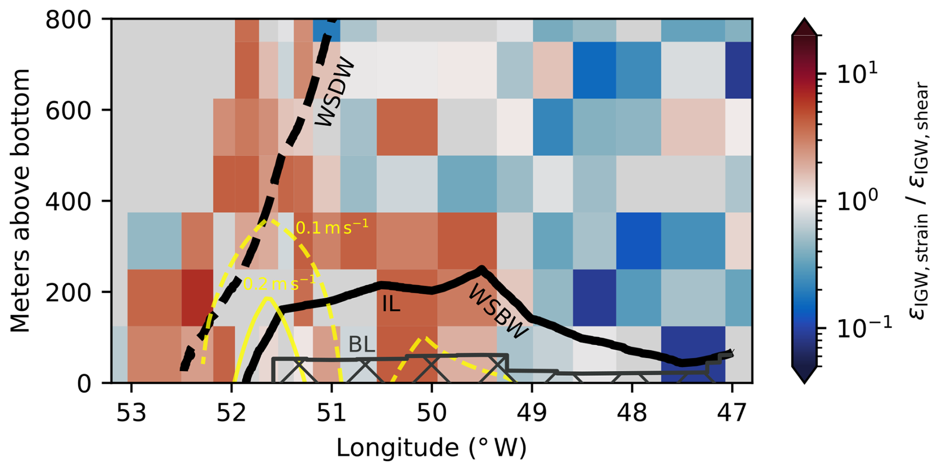
Figure D1 Ratio of fine-structure formulations on a logarithmic scale, calculated from measurements taken during the PS129 expedition. Isolines of mean absolute velocity (yellow) show the gravity current cores. Boundaries of water masses (WDW–WSDW, WSDW–WSBW) and gravity current layers (IL–BL) are drawn as lines. The bottom layer (BL) is hatched to indicate that the methods possibly break down in the nearly homogenously mixed layer.

The latitudinal correction L(f,N) is the same as in Eq. (10). The correction term h₁ differs from the corresponding term in Eq. (11) and Eq. (9), in the formulation dependent only on strain, but is instead as follows:

$$\begin{array}{}\text{(D2)}& h_{\mathrm{1}}\left(R_{\mathit{\omega }}\right)={\displaystyle \frac{\mathrm{3}\left(R_{\mathit{\omega }}+\mathrm{1}\right)}{\mathrm{2}\sqrt{\mathrm{2}}{R}_{\mathit{\omega }}\sqrt{R_{\mathit{\omega }}-\mathrm{1}}}}.\end{array}$$

The shear-to-strain variance ratio R_ω can be computed directly for every segment with

$$\begin{array}{}\text{(D3)}& R_{\mathit{\omega }}={\displaystyle \frac{〈U_z^{\mathrm{2}}〉}{\stackrel{\mathrm{‾}}{N^{\mathrm{2}}}\langle {\mathit{\zeta }}_z^{\mathrm{2}}\rangle }}\end{array}$$

and the segment-averaged vertical gradient of strain $\langle {\mathit{\zeta }}_z^{\mathrm{2}}\rangle$. Data from the PS129 expedition, where CTD and LADCP profiles were taken, allow us to compare both fine-structure formulations. The dissipation rate estimates from just strain (Eq. 9) and from shear and strain (Eq. D1) are denoted as ε_IGW,strain and ε_IGW,shear. Their ratio in the lowermost 800 m across the continental slope is displayed in Fig. D1. Across the continental slope and large parts of the gravity current, the strain-based formulation estimates higher dissipation rates than the shear-based formulation. In the open ocean, the strain-based formulation seems to underestimate the wave-induced turbulence in comparison to the shear-based results.