Dynamics of salt intrusion in complex estuarine networks: an idealised model applied to the Rhine–Meuse Delta

Many deltas in the world consist of a network of connected channels. We identify and quantify the characteristics of salt intrusion in such systems using an idealised model. The Rhine–Meuse Delta is selected as a prototype example of a complex network with many channels. The model is able to capture the characteristics of the tide-dominated water level variations due to the main tidal component and the salinity time series for 1 year of observations. Quantification of tidally averaged salt transport components shows that transport related to exchange flow is dominant in the seaward, deep parts of the network, but tidal dispersion is dominant in shallower channels further inland. Close to the network junctions, a tidally averaged downgradient salt transport is generated by the tidal currents, which is explained by the phase differences between the tidal currents in the different channels. Salt overspill is confined to the most seaward part of the Rhine–Meuse Delta. The magnitudes of the response times of different channels to changes in discharge increase with the distance to the estuary mouth and with decreasing net water transport through the channel. In channels without a subtidal discharge, response times are a factor of 2–4 larger than in the other channels. The effect of changes in the depth on the extent of salt intrusion strongly depends on where the change takes place. If the change is within the salt intrusion range, deepening will locally increase salt intrusion due to an increase in salt transport by the exchange flow. If the change is outside the salt intrusion range, changes to the net water transport dominate the response of the salt intrusion.

1 Introduction

The extent of salt intrusion into estuaries is changing worldwide as a result of climate change and anthropogenic activities. Climate change includes, for example, sea level rise (Qiu and Zhu, 2015) and changes in freshwater discharge (Bellafiore et al., 2021). Examples of anthropogenic activities are dam construction on rivers for water storage and hydropower generation (Qiu and Zhu, 2013), channel deepening for ship navigation, and construction of polders (Liu et al., 2019). The availability of theoretical frameworks to explain and of suitable models to simulate salt intrusion is crucial to predict how these changes affect the extent of salt intrusion.

For single-channel estuaries, relationships between estuarine geometry, forcing conditions, and salt intrusion are extensively studied. For this, theoretical frameworks (Geyer and MacCready, 2014), semi-empirical models (Savenije, 1993), idealised models (MacCready, 2004; Wei et al., 2022), models of intermediate complexity (Dijkstra and Schuttelaars, 2021), and detailed numerical models (Ralston et al., 2010; Martyr-Koller et al., 2017; Liu et al., 2024) are being used.

However, a number of estuaries consist of multiple channels. For these systems, also referred to as estuarine networks, the theories developed for single-channel estuaries need to be extended, as they behave differently in several ways. Observations show (Gong et al., 2014) that tidally averaged salt transport between channels through the junctions, a phenomenon known as salt overspill, occurs. Second, the phasing of tidal currents in estuarine networks creates local minima in the salt field (Warner et al., 2002; Garcia et al., 2022), which challenges the traditional view that salt transport by tides can be considered a dispersive process (Winterwerp, 1983). The implications of these phenomena for the large-scale salt dynamics are hard to determine from observations. Furthermore, unsteadiness of the salt field is known to be important in single-channel estuaries (e.g. Bowen and Geyer, 2003; Banas et al., 2004). For estuarine networks, Biemond et al. (2023) find that the interaction between channels depends on forcing conditions. Observations show that salt intrusion in some channels in the Mekong Delta changes substantially due to variation in tidal forcing over the spring–neap cycle, while other channels are less sensitive (Eslami et al., 2021). Using a 3D model, they explained this from differences in depth and stratification, but the interaction between the channels was not explicitly quantified. Next, the theory about the effect of changes to the geometry of estuaries does not contain all the relevant processes in estuarine networks. For example, Wu et al. (2016) suggest that the deepening of the North Passage, one of the channels of the Yangtze River Estuary, may have contributed to the salinity of the other channels. Liu et al. (2019) mention that channel deepening changed the amount of discharge reaching the Modaomen Waterway in the Pearl River Delta but that local channel deepening was more important to the salt intrusion.

Figure 1 Map of the Rhine–Meuse Delta. The inset shows the location in Europe. The bed level is indicated in Normaal Amsterdams Peil (NAP), which is a measure of the mean sea level. The yellow crosses indicate salinity observation points (a₁–a₈) and the red crosses water level observation points (b₁–b₁₉). Locations where both these quantities are measured or when these observation points are very close together are indicated by both colours.

Salt intrusion in estuarine networks has been studied using 1D models, for example, by Nguyen and Savenije (2006) and Zhang et al. (2011). Such models, when calibrated, have proven to be successful at predicting salt intrusion into estuaries, but their simplified nature does not allow the identification of the mechanisms of salt intrusion. On the other hand, 3D models have been used (e.g. Xue et al., 2009; Bricheno et al., 2021; Bellafiore et al., 2021), and while these models typically include realistic geometry and a wide range of physical processes that affect the salt transport, their high computational costs make extensive sensitivity studies computationally unfeasible. To fill the gap between simple 1D models and 3D numerical models of estuarine networks, we develop here an idealised, partly analytical, width-averaged (2DV) model. This model is suitable for a process-based analysis of salt intrusion mechanisms, as the model solves separately for different components of currents and salinity, which makes the computation of different components of the salt transport straightforward. Furthermore, it has lower computational costs than a 3D numerical model and it is easier to implement features such as estuarine network geometry.

To study the characteristics of salt intrusion in estuarine networks, the model will be applied to the Rhine–Meuse Delta (the Netherlands) (RMD), which is formed by the outflow of the Rhine and Meuse rivers discharging into the North Sea (Fig. 1). The current geometry of the delta is to a large extent anthropogenically determined (Cox et al., 2021), with the large harbour of Rotterdam situated in the seaward part. Earlier research on salt intrusion into this system by de Nijs and Pietrzak (2012) using measurements and 3D model simulations revealed that intertidal transport of salt between the channels occurs, but the effects of this transport on the tidally averaged salinity were not quantified. Recently, salt intrusion into the RMD has received increased attention. Kranenburg et al. (2022) showed that upstream salt transport is dominated by exchange flow in the seaward part and by tidal currents in the landward part of one of the major branches but that during storm surges, the relative importance of the different mechanisms changes. Wullems et al. (2023) point to the dependency of salinity on water level at one location in the network, using a data-driven method. None of these studies provide a network-wide analysis of salt intrusion.

To systematically investigate the dynamics of salt intrusion in estuarine networks, we formulate four specific aims:

1. to show that a calibrated, idealised 2DV model successfully hindcasts hydrodynamics and salinity in an estuarine network;

2. to identify and quantify the different salt transport processes in an estuarine network and highlight the differences from single-channel estuaries;

3. to quantify the time-dependent response to changes in discharge in an estuarine network;

4. to quantify the effects of changes in the depth of individual channels on salt intrusion into the major branches of an estuarine network.

The remainder of this paper is organised as follows. In Sect. 2, the model, its implementation in the RMD, and the set-up of the simulations are described. Section 3 presents results focused on the four specific aims. Section 4 discusses the results, and Sect. 5 presents the conclusions.

2 Model formulation

2.1 Model approach

The model chosen to address the research questions is an exploratory model. This type of model is simplified where possible, such that it only contains the essential ingredients to describe the relevant physics (Murray, 2003). The simplifications aim to isolate poorly understood phenomena, in this case, salt intrusion into estuarine networks. An additional advantage is that due to the lower computational demand, parameter sensitivity studies are easy to perform. Successful examples of this approach in the context of salt intrusion can be found in, for example, MacCready (2004), Chen (2015), and Wei et al. (2016). Detailed quantitative agreement with observations is not the primary goal of this type of models. However, to assure that the right part of the parameter space is investigated, we will calibrate the model parameters using a model–observation comparison. The simplifications in the model primarily concern the geometry, concern the turbulence closure, and disregarded physical processes. In the model description in the remainder of this section, simple formulations of these aspects will be used. The consequences of the assumptions on which these formulations are built will be addressed in the discussion section.

2.2 Domain

The domain mimics an estuarine network that has a number of width-averaged channels, which are connected to each other through a set of junctions. As a specific example, Fig. 2 shows the representation of the RMD network. There are four types of horizontal boundaries for the channels: river boundaries, weir boundaries, sea boundaries (estuary mouths), and junctions. Salt enters through the sea boundaries. Fresh water enters (or leaves, for example, in the case of the Haringvliet sluices) through the river and weir boundaries. The junctions provide the connections between the channels.

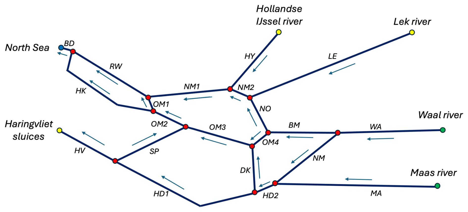
Figure 2 Representation of the RMD channel network in the model. Black lines indicate channels, blue arrows indicate the direction of the local x axis, red dots indicate junctions, yellow dots indicate weir boundaries, green dots indicate river boundaries, and blue dots indicate sea boundaries. Table A1 provides the meaning of the acronyms for the channels.

Each channel i is divided into a number of segments j, which have different constant depths H_ij. Locations in the segments are characterised by a horizontal coordinate x_ij, which runs from −L_ij to 0, and by a vertical coordinate z_ij that runs from the bottom $z_{ij}=-H_{ij}$ to the water surface z_ij=η_ij, while the undisturbed water level is at z_ij=0. By convention, x_ij increases in the direction of the time- and cross-sectionally averaged flow for yearly averaged discharge conditions (indicated by arrows in Fig. 2). For clarity, the subscript ij will be left out from now on, and the equations shown are valid for each segment. The width of each segment is described as

$$\begin{array}{}\text{(1)}& b\left(x\right)=b(x=-L)e^{(x+L)/L_b},\end{array}$$

where L_b is an e-folding length scale that describes the width convergence. The width is continuous at the boundaries of the segments but not necessarily at the junctions.

2.3 Equations of motion

The governing equations for hydrodynamics and salinity are described in Biemond et al. (2024a). The model is width averaged, and in this domain, momentum and continuity balances are solved for hydrodynamics, and a mass balance is solved for salinity. Water level η, horizontal and vertical velocity u and w, and salinity s are decomposed into tidally varying (indicated by the subscript ti) and subtidal (indicated by the subscript st) components. Subtidal horizontal velocity and salinity are further decomposed into a depth-averaged component (indicated by an overbar) and a depth-dependent component (indicated by a prime). This yields

$$\begin{array}{}\text{(2)}& \begin{array}{rl}& \mathit{\eta }={\mathit{\eta }}_{\mathrm{st}}+{\mathit{\eta }}_{\mathrm{ti}},u={\stackrel{\mathrm{‾}}{u}}_{\mathrm{st}}+u_{\mathrm{st}}^{\prime }+u_{\mathrm{ti}},\\ & w=w_{\mathrm{st}}+w_{\mathrm{ti}},s={\stackrel{\mathrm{‾}}{s}}_{\mathrm{st}}+s_{\mathrm{st}}^{\prime }+s_{\mathrm{ti}}.\end{array}\end{array}$$

Analytical solutions to the dominant tidally averaged momentum and mass balances are found, which yield expressions for the subtidal water level gradient $\frac{\partial {\mathit{\eta }}_{\mathrm{st}}}{\partial x}$, the depth-averaged and depth-varying components of the subtidal horizontal velocity u_st and vertical velocity w_st. They read

$$\begin{array}{}\text{(3a)}& {\displaystyle \frac{\partial {\mathit{\eta }}_{\mathrm{st}}}{\partial x}}=-{\displaystyle \frac{\mathrm{6}}{\mathrm{5}}}{\displaystyle \frac{A_{\mathrm{v},\mathrm{st}}Q}{gb{H}^{\mathrm{3}}}},\text{(3b)}& {\displaystyle }{\stackrel{\mathrm{‾}}{u}}_{\mathrm{st}}={\displaystyle \frac{Q}{bH}},\text{(3c)}& {\displaystyle }{u}_{\mathrm{st}}^{\prime }={\displaystyle \frac{Q}{bH}}{P}_{\mathrm{1}}\left(\stackrel{\mathrm{̃}}{z}\right)+{\displaystyle \frac{g\mathit{\beta }{H}^{\mathrm{3}}}{\mathrm{48}{A}_{\mathrm{v},\mathrm{st}}}}{\displaystyle \frac{\partial {\overline{s}}_{\mathrm{st}}}{\partial x}}{P}_{\mathrm{2}}\left(\stackrel{\mathrm{̃}}{z}\right),\text{(3d)}& {\displaystyle }{w}_{\mathrm{st}}=-{\displaystyle \frac{g\mathit{\beta }{H}^{\mathrm{4}}}{\mathrm{48}{A}_{\mathrm{v},\mathrm{st}}}}({\displaystyle \frac{{\partial }^{\mathrm{2}}{\overline{s}}_{\mathrm{st}}}{\partial x^{\mathrm{2}}}}+L_b^{-\mathrm{1}}{\displaystyle \frac{\partial {\overline{s}}_{\mathrm{st}}}{\partial x}})P_w\left(\stackrel{\mathrm{̃}}{z}\right).\end{array}$$

Here, Q is net water transport, g=9.81 m s⁻² is gravitational acceleration, $\mathit{\beta }=\mathrm{7.6}\times {\mathrm{10}}^{-\mathrm{4}}$ (g kg⁻¹)⁻¹ is the isohaline contraction coefficient, and A_v,st is the vertical eddy viscosity acting on the subtidal flow. The quantity $\frac{\partial {\mathit{\eta }}_{\mathrm{st}}}{\partial x}$ is required to calculate the water distribution in the channels, and similarly, w_st is required for the vertical structure of the subtidal salinity field $s_{\mathrm{st}}^{\prime }$. Note that we have neglected the contribution of salinity to the subtidal water level gradient because taking it into account would introduce a strong relationship between salinity and net water transport, which is not realistic (Buschman et al., 2010; Maicu et al., 2018; Wang et al., 2021). Polynomials P₁, P₂, and P_w describe the vertical structure of the flow and depend on the normalised vertical coordinate $\stackrel{\mathrm{̃}}{z}=\frac{z}{H}$. They are defined as

$$\begin{array}{}\text{(4)}& \begin{array}{rl}& P_{\mathrm{1}}\left(\stackrel{\mathrm{̃}}{z}\right)=({\displaystyle \frac{\mathrm{1}}{\mathrm{5}}}-{\displaystyle \frac{\mathrm{3}}{\mathrm{5}}}{\stackrel{\mathrm{̃}}{z}}^{\mathrm{2}}),P_{\mathrm{2}}\left(\stackrel{\mathrm{̃}}{z}\right)=({\displaystyle \frac{\mathrm{8}}{\mathrm{5}}}-{\displaystyle \frac{\mathrm{54}}{\mathrm{5}}}{\stackrel{\mathrm{̃}}{z}}^{\mathrm{2}}-\mathrm{8}{\stackrel{\mathrm{̃}}{z}}^{\mathrm{3}}),\\ & P_w\left(\stackrel{\mathrm{̃}}{z}\right)=(\mathrm{2}{\stackrel{\mathrm{̃}}{z}}^{\mathrm{4}}+{\displaystyle \frac{\mathrm{18}}{\mathrm{5}}}{\stackrel{\mathrm{̃}}{z}}^{\mathrm{3}}-{\displaystyle \frac{\mathrm{8}}{\mathrm{5}}}\stackrel{\mathrm{̃}}{z}).\end{array}\end{array}$$

The water level η_ti, horizontal velocity component u_ti, and vertical velocity component w_ti of the tidally varying flow field read

$$\begin{array}{}\text{(5a)}& {\displaystyle }({\mathit{\eta }}_{\mathrm{ti}},u_{\mathrm{ti}},w_{\mathrm{ti}})=\mathrm{\Re }\mathit{\left\{}\right({\widehat{\mathit{\eta }}}_{\mathrm{ti}},{\widehat{u}}_{\mathrm{ti}},{\widehat{w}}_{\mathrm{ti}}\left)\exp \right(i\mathit{\omega }t\left)\mathit{\right\}},\text{(5b)}& {\displaystyle }\begin{array}{rl}{\widehat{\mathit{\eta }}}_{\mathrm{ti}}=\exp & \left(-{\displaystyle \frac{(x+L)}{\mathrm{2}{L}_b}}\right)\\ & \left(C_{\mathrm{1}}\exp \left(k\right(x+L\left)\right)+C_{\mathrm{2}}\exp (-k(x+L\left)\right)\right),\end{array}\text{(5c)}& {\displaystyle }{\widehat{u}}_{\mathrm{ti}}={\displaystyle \frac{g}{i\mathit{\omega }}}{\displaystyle \frac{\partial {\widehat{\mathit{\eta }}}_{\mathrm{ti}}}{\partial x}}\left(B\cosh \left({\mathit{\delta }}_A{\displaystyle \frac{z}{H}}\right)-\mathrm{1}\right),\text{(5d)}& {\displaystyle }\begin{array}{rl}{\widehat{w}}_{\mathrm{ti}}=i\mathit{\omega }{\widehat{\mathit{\eta }}}_{\mathrm{ti}}-{\displaystyle \frac{g}{i\mathit{\omega }}}& \left({\displaystyle \frac{d^{\mathrm{2}}{\widehat{\mathit{\eta }}}_{\mathrm{ti}}}{\mathrm{d}{x}^{\mathrm{2}}}}+{\displaystyle \frac{\mathrm{1}}{L_b}}{\displaystyle \frac{\mathrm{d}{\widehat{\mathit{\eta }}}_{\mathrm{ti}}}{\mathrm{d}x}}\right)\\ & \left({\displaystyle \frac{BH}{{\mathit{\delta }}_A}}\sinh \left({\mathit{\delta }}_A{\displaystyle \frac{z}{H}}\right)-z\right).\end{array}\end{array}$$

Here, ω is the angular frequency of the tidal constituent that is considered, t is time, L is the length of a channel segment, ℜ denotes the real part of a complex variable, and C₁ and C₂ are determined by the horizontal boundary conditions and represent tidal waves that travel downstream and upstream, respectively. The other parameters are defined as

$$\begin{array}{}\text{(6)}& \begin{array}{rl}& {\mathit{\delta }}_A={\displaystyle \frac{(\mathrm{1}+i)H}{\sqrt{\frac{\mathrm{2}{A}_{\mathrm{v},\mathrm{ti}}}{\mathit{\omega }}}}},B=\left(\cosh \right({\mathit{\delta }}_A)+{\displaystyle \frac{{\mathit{\delta }}_A}{\mathrm{2}}}\sinh ({\mathit{\delta }}_A){)}^{-\mathrm{1}},\\ & k=\sqrt{{\displaystyle \frac{\mathrm{1}}{(\mathrm{2}{L}_b{)}^{\mathrm{2}}}}+{\displaystyle \frac{{\mathit{\omega }}^{\mathrm{2}}}{gH}}{\left({\displaystyle \frac{B}{{\mathit{\delta }}_A\sinh \left({\mathit{\delta }}_A\right)}}-\mathrm{1}\right)}^{-\mathrm{1}}},\end{array}\end{array}$$

in which A_v,ti is the vertical eddy viscosity acting on the tidal flow. Note that we split subtidal horizontal velocity into a depth-averaged and a depth-dependent component but do not make this separation for tidal velocity. Furthermore, A_v,ti and therefore u_ti do not depend on salinity.

For salinity, no analytical expressions are obtained, but the decomposition from Eq. (2) is substituted in the 2DV mass balance for salinity, which reads

$$\begin{array}{}\text{(7)}& \begin{array}{rl}{\displaystyle \frac{\partial s}{\partial t}}& +{\displaystyle \frac{\mathrm{1}}{b}}{\displaystyle \frac{\partial }{\partial x}}\left(bus\right)+{\displaystyle \frac{\partial }{\partial z}}\left(ws\right)\\ & ={\displaystyle \frac{\mathrm{1}}{b}}{\displaystyle \frac{\partial }{\partial x}}\left(b{K}_{\mathrm{h}}{\displaystyle \frac{\partial s}{\partial x}}\right)+{\displaystyle \frac{\partial }{\partial z}}\left(K_{\mathrm{v}}{\displaystyle \frac{\partial s}{\partial z}}\right).\end{array}\end{array}$$

Here, K_h is the horizontal dispersion coefficient, and K_v is the vertical eddy diffusivity coefficient. To obtain an equation for subtidal depth-averaged salinity ${\stackrel{\mathrm{‾}}{s}}_{\mathrm{st}}$, we average this equation over depth and the tidal timescale, which gives

$$\begin{array}{}\text{(8)}& \begin{array}{rl}{\displaystyle \frac{\partial {\stackrel{\mathrm{‾}}{s}}_{\mathrm{st}}}{\partial t}}& +{\stackrel{\mathrm{‾}}{u}}_{\mathrm{st}}{\displaystyle \frac{\partial {\stackrel{\mathrm{‾}}{s}}_{\mathrm{st}}}{\partial x}}+\stackrel{\mathrm{‾}}{u_{\mathrm{st}}^{\prime }{\displaystyle \frac{\partial s_{\mathrm{st}}^{\prime }}{\partial x}}}+{\left({\stackrel{\mathrm{‾}}{u}}_{\mathrm{ti}}{\displaystyle \frac{\partial {\stackrel{\mathrm{‾}}{s}}_{\mathrm{ti}}}{\partial x}}\right)}_{\mathrm{st}}+{\left(\stackrel{\mathrm{‾}}{u_{\mathrm{ti}}^{\prime }{\displaystyle \frac{\partial s_{\mathrm{ti}}^{\prime }}{\partial x}}}\right)}_{\mathrm{st}}\\ & ={\displaystyle \frac{\mathrm{1}}{b}}{\displaystyle \frac{\partial }{\partial x}}\left(b{K}_{\mathrm{h},\mathrm{st}}{\displaystyle \frac{\partial {\stackrel{\mathrm{‾}}{s}}_{\mathrm{st}}}{\partial x}}\right).\end{array}\end{array}$$

In this expression, K_h,st is the horizontal dispersion coefficient acting on the subtidal salinity. The equation for the vertically varying part of the subtidal salinity $s_{\mathrm{st}}^{\prime }$, obtained from subtracting Eq. (8) from the tidally averaged mass balance, reads

$$\begin{array}{}\text{(9)}& \begin{array}{rl}{\displaystyle \frac{\partial s_{\mathrm{st}}^{\prime }}{\partial t}}& +{\stackrel{\mathrm{‾}}{u}}_{\mathrm{st}}{\displaystyle \frac{\partial s_{\mathrm{st}}^{\prime }}{\partial x}}+u_{\mathrm{st}}^{\prime }{\displaystyle \frac{\partial {\stackrel{\mathrm{‾}}{s}}_{\mathrm{st}}}{\partial x}}+u_{\mathrm{st}}^{\prime }{\displaystyle \frac{\partial s_{\mathrm{st}}^{\prime }}{\partial x}}-\stackrel{\mathrm{‾}}{u_{\mathrm{st}}^{\prime }{\displaystyle \frac{\partial s_{\mathrm{st}}^{\prime }}{\partial x}}}+w_{\mathrm{st}}{\displaystyle \frac{\partial s_{\mathrm{st}}^{\prime }}{\partial z}}\\ & +{\left({\stackrel{\mathrm{‾}}{u}}_{\mathrm{ti}}{\displaystyle \frac{\partial s_{\mathrm{ti}}^{\prime }}{\partial x}}\right)}_{\mathrm{st}}+{\left(u_{\mathrm{ti}}^{\prime }{\displaystyle \frac{\partial {\stackrel{\mathrm{‾}}{s}}_{\mathrm{ti}}}{\partial x}}\right)}_{\mathrm{st}}+{\left(u_{\mathrm{ti}}^{\prime }{\displaystyle \frac{\partial s_{\mathrm{ti}}^{\prime }}{\partial x}}\right)}_{\mathrm{st}}\\ & -{\left(\stackrel{\mathrm{‾}}{u_{\mathrm{ti}}^{\prime }{\displaystyle \frac{\partial s_{\mathrm{ti}}^{\prime }}{\partial x}}}\right)}_{\mathrm{st}}+{\left(w_{\mathrm{ti}}{\displaystyle \frac{\partial s_{\mathrm{ti}}^{\prime }}{\partial z}}\right)}_{\mathrm{st}}\\ & ={\displaystyle \frac{\mathrm{1}}{b}}{\displaystyle \frac{\partial }{\partial x}}\left(b{K}_{\mathrm{h},\mathrm{st}}{\displaystyle \frac{\partial s_{\mathrm{st}}^{\prime }}{\partial x}}\right)+{\displaystyle \frac{\partial }{\partial z}}\left(K_{\mathrm{v},\mathrm{st}}{\displaystyle \frac{\partial s_{\mathrm{st}}^{\prime }}{\partial z}}\right).\end{array}\end{array}$$

Here, K_v,st is the vertical eddy diffusivity coefficient acting on the subtidal salinity. An equation for tidally varying salinity s_ti is obtained by subtracting the tidally averaged mass balance from the full mass balance. Additionally, only the dominant tidal constituent is considered, i.e. $s_{\mathrm{ti}}=\mathrm{\Re }\left[{\widehat{s}}_{\mathrm{ti}}\exp (-i\mathit{\omega }t)+c.c.\right]$, and a scaling analysis is applied to select the most important terms. The equation governing the dynamics of ${\widehat{s}}_{\mathrm{ti}}$ is

$$\begin{array}{}\text{(10)}& -i\mathit{\omega }{\widehat{s}}_{\mathrm{ti}}+{\widehat{u}}_{\mathrm{ti}}{\displaystyle \frac{\partial {\stackrel{\mathrm{‾}}{s}}_{\mathrm{st}}}{\partial x}}+{\widehat{w}}_{\mathrm{ti}}{\displaystyle \frac{\partial s_{\mathrm{st}}^{\prime }}{\partial z}}={\displaystyle \frac{\partial }{\partial z}}\left(K_{\mathrm{v},\mathrm{ti}}{\displaystyle \frac{\partial {\widehat{s}}_{\mathrm{ti}}}{\partial z}}\right),\end{array}$$

in which K_v,ti is the vertical eddy diffusivity coefficient acting on the tidally varying salinity. This equation has an analytical solution (i.e. ${\widehat{s}}_{\mathrm{ti}}$ can be expressed as a function of s_st), but this expression is very lengthy and therefore not presented here. To numerically solve for ${\stackrel{\mathrm{‾}}{s}}_{\mathrm{st}}$ and $s_{\mathrm{st}}^{\prime }$, a Galerkin method is used in the vertical and central differences in the horizontal. For time integration, a backward Euler scheme is employed.

The values of the vertical eddy viscosity, vertical eddy diffusivity, and horizontal dispersion coefficients are assumed to be constant throughout the entire domain. For bottom friction, a partial slip condition is applied at the bed, with a friction coefficient $S_{\mathrm{f}}=\frac{\mathrm{2}{A}_{\mathrm{v}}}{H}$, where A_v is the vertical eddy viscosity, and H is the water depth. Note that the values of the coefficients used for eddy viscosity, eddy diffusivity, dispersion, and friction depend on whether they act on the tidal or subtidal current and salinity, as is explained in, for example, Godin (1991, 1999).

2.4 Salt transport

The horizontal salt transport T in the model (which follows from the decomposition of currents and salinity as in Eq. 2), integrated over the tidal cycle and cross-section and after neglecting terms that contain η (see Biemond et al., 2024a), reads

$$\begin{array}{}\text{(11)}& T=\underset{{\text{T}}_Q}{\underbrace{\phantom{{\displaystyle \frac{\mathrm{1}}{\mathrm{1}}}}Q{\stackrel{\mathrm{‾}}{s}}_{\mathrm{st}}}}+\underset{{\text{T}}_{\mathrm{E}}}{\underbrace{\phantom{{\displaystyle \frac{\mathrm{1}}{\mathrm{1}}}}bH\stackrel{\mathrm{‾}}{u_{\mathrm{st}}^{\prime }{s}_{\mathrm{st}}^{\prime }}}}+\underset{{\text{T}}_T}{\underbrace{\phantom{{\displaystyle \frac{\mathrm{1}}{\mathrm{1}}}}bH{\stackrel{\mathrm{‾}}{\left(u_{\mathrm{ti}}{s}_{\mathrm{ti}}\right)}}_{\mathrm{st}}}}-\underset{{\text{T}}_{\mathrm{D}}}{\underbrace{\phantom{{\displaystyle \frac{\mathrm{1}}{\mathrm{1}}}}bH{K}_{\mathrm{h},\mathrm{st}}{\displaystyle \frac{\partial {\stackrel{\mathrm{‾}}{s}}_{\mathrm{st}}}{\partial x}}}}.\end{array}$$

The component T_Q is the salt transport due to advection by the depth-averaged subtidal current, T_E is the salt transport by the exchange flow, T_T is the salt transport due to the time correlation of tidal flow and salinity, and T_D is the salt transport due to horizontal dispersion. In our model, unresolved upstream salt transport processes are parametrised by the last term. Note that T_T could be further decomposed into a contribution that involves only the depth-averaged tidal current and a contribution that is due to the departure of the tidal current from its depth-averaged value.

2.5 Boundary conditions

Regarding the boundary conditions at river boundaries, subtidal discharge is prescribed, tides are assumed to dissipate in the river beyond the boundary (without reflection at a horizontal boundary), and the subtidal salinity is set to the river salinity. Hence,

$$\begin{array}{}\text{(12)}& bH{\stackrel{\mathrm{‾}}{u}}_{\mathrm{st}}=Q_{\mathrm{riv}},C_{\mathrm{1}}=\mathrm{0},{\stackrel{\mathrm{‾}}{s}}_{\mathrm{st}}=s_{\mathrm{riv}},s_{\mathrm{st}}^{\prime }=\mathrm{0}.\end{array}$$

Here, Q_riv and s_riv are the river discharge and salinity, respectively, which are generally non-zero. The condition C₁=0 means that there is no downstream travelling tidal wave.

At the weir boundaries, we prescribe subtidal discharge and use a reflecting boundary condition for the tidal flow such that the water transport vanishes at such boundaries. For salinity, we impose conditions on the salt transport. When the discharge at the weir is into the domain (which is usually the case), the depth-averaged transport equals the prescribed salinity s_weir multiplied by the discharge. When the discharge at the weir is out of the domain (which is the case for the Haringvliet sluices in the RMD, for example), the depth-averaged transport is set to the calculated salinity at the weir multiplied by the discharge. The vertical variations in the dispersive salt flux are set to zero to avoid the formation of a dispersive boundary layer (Biemond et al., 2024b). In summary, the boundary conditions read

$$\begin{array}{}\text{(13)}& \begin{array}{rl}& bH{\stackrel{\mathrm{‾}}{u}}_{\mathrm{st}}=Q_{\mathrm{weir}},\underset{-H}{\overset{\mathrm{0}}{\int }}{u}_{\mathrm{ti}}\mathrm{d}z=\mathrm{0},\\ & T=Q_{\mathrm{weir}}{s}_{\mathrm{weir}},K_{\mathrm{h},\mathrm{st}}{\displaystyle \frac{\partial s_{\mathrm{st}}^{\prime }}{\partial x}}=\mathrm{0},\end{array}\end{array}$$

in which Q_weir is the discharge at the weir, and s_weir is prescribed in the case of the discharge being from the weir and is the local (depth-averaged) salinity in the case of a discharge towards the weir.

Water levels η_st and η_ti are prescribed at sea boundaries (estuary mouths). To obtain the conditions for salinity, additional segments are added that extend seaward from the mouths. These segments are characterised by strongly increasing widths away from the mouths. At the outer sea boundaries of these segments, salinity is set to the sea salinity. Furthermore, the assumption that there is only an incoming tidal wave at these locations (i.e. travelling from sea to estuary) allows us to compute the water levels and tidal flow in these segments. The assumption made here is reasonable because of the strongly increasing width of these segments.

At the junctions, continuity of discharge and water level is imposed. These conditions apply to the subtidal quantities as well as to the tidally varying quantities. Regarding salinity, continuity of salt transport and salinity is used at every vertical level. To apply conditions to the tidal salinity, a boundary layer correction is employed. At the boundaries between the channel segments, the same conditions are applied. The specific expressions for these boundary conditions are described in Appendix B, and the boundary layer correction for tidal salinity is described in Appendix C.

2.6 Model implementation for the RMD

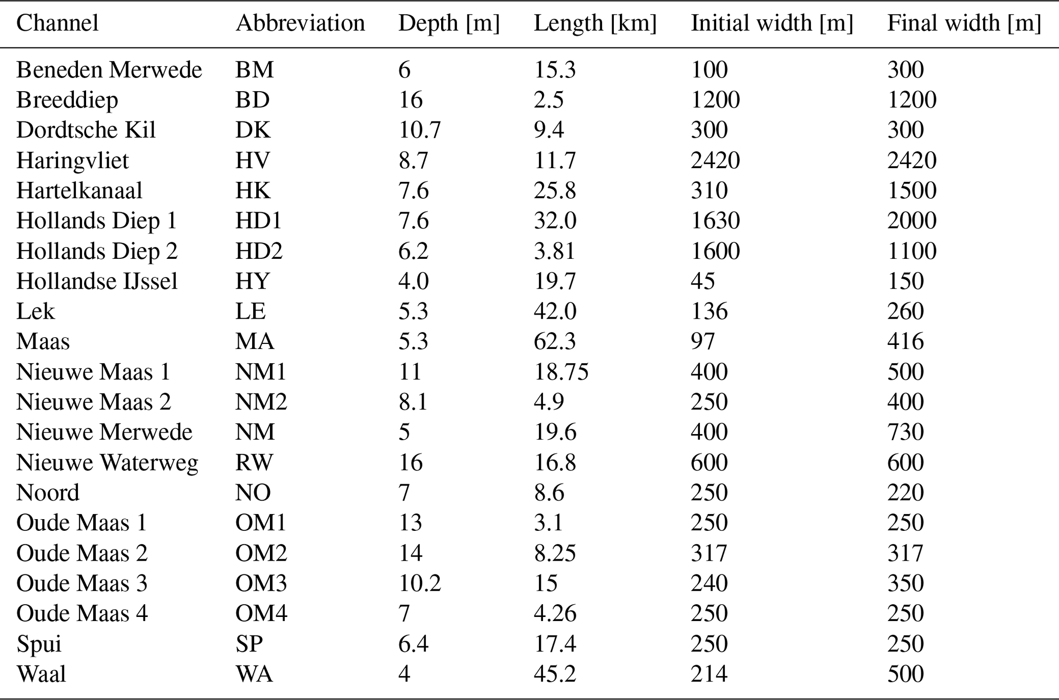
The implementation of the domain of the RMD in the model, as sketched in Fig. 2, consists of 21 channels, 12 junctions, 1 sea boundary, 3 weir boundaries, and 2 river boundaries. The channels consist of one or two segments. The division into multiple segments is based on the desired horizontal grid size and does not affect the physics. The Haringvliet sluices connect the Haringvliet to the open sea and are only opened to release water from the Haringvliet such that no salt intrudes through this boundary. The widths and depths of each channel are presented in Table A1. Note that a coarse representation of the geometry is used, so geometrical details (e.g. the harbour basins) are not resolved. In the following, we will refer to the different channels by the acronyms specified in Fig. 2.

The horizontal grid size is around a few hundred metres but differs per channel and is finer in regions where larger salinity gradients are expected. In the vertical, five Fourier modes are used for the Galerkin projection, and the model time step (which only applies to subtidal quantities) is 24 h.

The model is forced with prescribed time series of discharge at the two river and the three weir boundaries and with the water level amplitude and phase of the dominant tidal constituent, which is the semi-diurnal lunar M₂ tide (period 12 h, 25 m) for the RMD at the North Sea boundary (note that the water level amplitude of the M₂ component at the station at the mouth (b₁) is 4 times larger than that of the second-largest component; Walters, 1987). For salinity, time-independent values are used, which are 0.15 g kg⁻¹ at the river and weir boundaries and 33 g kg⁻¹ at the North Sea boundary.

Figure 3 (a) Observed (in blue) and modelled (in red) amplitudes of the M₂ water level for different points in the RMD, the locations of which are indicated in Fig. 1. (b) As (a), but for the tidal phase of the water level.

3 Results

3.1 Model–observation comparison

3.1.1 Method

To address the first aim (model–observation comparison), suitable values of eddy viscosity, eddy diffusivity, and dispersion coefficients are needed. This is achieved by means of calibration: the modelled tidal water levels and salinities are compared to observed tidal water levels and salinities. There are 19 water level stations in the RMD, indicated by b₁–b₁₉ in Fig. 1, and 7 salinity observation points, indicated by a₁–a₇ in this figure. At a number of these locations, salinity observations are available at two or three depths. There are only a few permanent current measurement stations available in the RMD, and therefore currents are not evaluated. The discharge, water level, and salinity data of the RMD are accessible at https://waterinfo.rws.nl, last access: 31 January 2024. The year 2022 is used as calibration period since this is a year with a low Rhine discharge, which is a situation in which salt intrusion is relevant. For the hydrodynamic module, the vertical eddy viscosity component acting on the tidal flow A_v,ti is calibrated. An optimisation procedure is employed for this variable to find the minimum error between the modelled and the observed M₂ water level variations, using the skill score as used by Davies and Jones (1996), which computes a cost function f as

$$\begin{array}{}\text{(14)}& f=\sum _{k=\mathrm{1}}^N\sqrt{{\left({\widehat{\mathit{\eta }}}_k^{\mathrm{obs}}-{\widehat{\mathit{\eta }}}_k^{\mathrm{mod}}\right)}^{\mathrm{2}}+\mathrm{2}{\widehat{\mathit{\eta }}}_k^{\mathrm{obs}}{\widehat{\mathit{\eta }}}_k^{\mathrm{mod}}\left(\mathrm{1}-\cos \left({\widehat{\mathit{\theta }}}_k^{\mathrm{obs}}-{\widehat{\mathit{\theta }}}_k^{\mathrm{mod}}\right)\right)}.\end{array}$$

Here, N is the number of observations; ${\widehat{\mathit{\eta }}}_k^{\mathrm{obs}}$ and ${\widehat{\mathit{\eta }}}_k^{\mathrm{mod}}$ are the observed and modelled amplitudes of the water level of the dominant tidal constituent, respectively; and ${\widehat{\mathit{\theta }}}_k^{\mathrm{obs}}$ and ${\widehat{\mathit{\theta }}}_k^{\mathrm{mod}}$ are the observed and modelled phases of the tidal water level, respectively.

The coefficients for subtidal vertical eddy viscosity A_v,st, subtidal vertical eddy diffusivity K_v,st, horizontal dispersion K_h,st, and tidal vertical eddy diffusivity K_v,ti are calibrated by minimising the root-mean-squared error (RMSE) between observed and modelled time series of subtidal salinity at the observations points. A gradient descent algorithm is employed to find the optimal values of these parameters. After the calibration, the model performance regarding subtidal salinity is quantified by calculating the Nash–Sutcliffe efficiency (NSE) (Nash and Sutcliffe, 1970), which reads

$$\begin{array}{}\text{(15)}& \mathrm{NSE}=\mathrm{1}-{\displaystyle \frac{{\sum }_{k=\mathrm{1}}^N{\left(s_k^{\mathrm{obs}}-s_k^{\mathrm{mod}}\right)}^{\mathrm{2}}}{{\sum }_{k=\mathrm{1}}^N{\left(s_k^{\mathrm{obs}}-<s_k^{\mathrm{obs}}>\right)}^{\mathrm{2}}}},\end{array}$$

where $s_k^{\mathrm{obs}}$ and $s_k^{\mathrm{mod}}$ are the observed and modelled salinity, respectively, and $<\cdot >$ indicates a time-averaged quantity. A score of NSE =1 indicates perfect agreement, while NSE =0 means that the model error is equal to the variance of the observed time series, and finally NSE <0 indicates that the observed mean is a better predictor than the model.

3.1.2 Tides

The amplitudes and phases of the M₂ component of the water level in observations and of the calibrated model are shown in Fig. 3. A minimum for f is obtained with $A_{\mathrm{v},\mathrm{ti}}=\mathrm{0.025}$ m² s⁻¹. The amplitude in the main channels is well-resolved (b₁–b₇, b₁₂–b₁₄). At observation point b₉ (the LE channel), the amplitude is underestimated by 27 %, and in the southern part (b₁₆–b₁₉), the amplitude is overestimated by 55 % averaged over the four points. There are two outliers in terms of tidal phases (at points b₅ and b₁₆). The observed phase at point b₅ differs in such a way from the phase at the neighbouring points that an error in the raw data is probably responsible for the mismatch here. At point b₁₆, the tides are affected by the operation of the Haringvliet sluices, which is not resolved in the model.

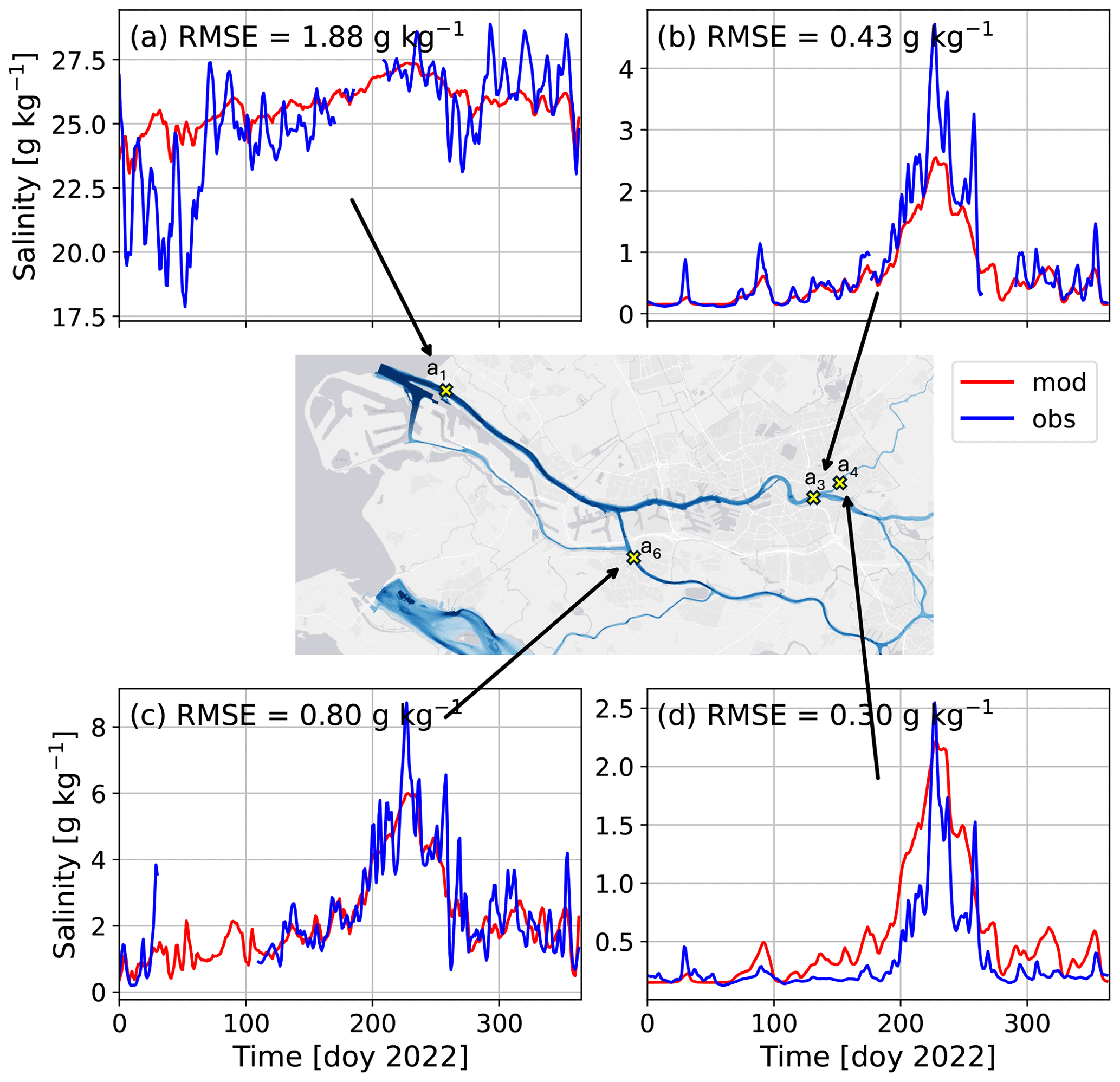
Figure 4 Observed (in blue) and modelled (in red) tidally averaged salinity time series for 2022 at four locations in the RMD: (a) a₁ ($z=-\mathrm{9.0}$ m), (b) a₃ ($z=-\mathrm{2.5}$ m), (c) a₆ ($z=-\mathrm{2.5}$ m), and (d) a₄ ($z=-\mathrm{4.0}$ m).

3.1.3 Salinity

The NSE (Eq. 15) for the modelled and observed salinity after calibration is 0.67, which classifies the model performance as satisfactory (Moriasi et al., 2015). This result is found for $A_{\mathrm{v},\mathrm{st}}=\mathrm{0.0024}$ m² s⁻¹, an order of magnitude lower than the vertical eddy viscosity for tidal flow. Regarding vertical eddy diffusivities for tidal and subtidal salinity, the best agreement is found when using $K_{\mathrm{v},\mathrm{st}}=\frac{A_{\mathrm{v},\mathrm{st}}}{\mathit{Sc}}$ and $K_{\mathrm{v},\mathrm{ti}}=\frac{A_{\mathrm{v},\mathrm{ti}}}{\mathit{Sc}}$, with Sc, the Schmidt number, equal to 2.2. The horizontal subtidal dispersion coefficient is $K_{\mathrm{h},\mathrm{st}}=\mathrm{275}$ m² s⁻¹, which is rather high compared to what was found for single-channel estuaries (Biemond et al., 2024a). The reasons for and implications of this will be discussed in Sect. 4.

Modelled and observed salinity in the RMD at four selected observation points is shown in Fig. 4. We refer to Fig. S1 for the comparison at the other observations points. Differences between the model and observations primarily concern an underestimation of the variability in the salt field. This is due to the fact that our model does not account for the spring–neap tidal cycle, overtides, and subtidal and intratidal water level fluctuations at the sea boundary driven by remote winds, which have a strong influence on the variability in the salinity. The model–data agreement is consistent at different depths for most stations where observations are available at multiple depths (Fig. S1), but the salinity at station a₁ is underestimated by 3.0 g kg⁻¹ at $z=-\mathrm{9.0}$ m averaged over first 2 months of the year (i.e. during high-discharge conditions), while at $z=-\mathrm{2.5}$ m, no bias is present (compare Fig. S1b with Fig. S1d). This indicates that the relation between discharge and vertical salinity gradients in the model is not well resolved, which is probably due to the use of a constant vertical eddy viscosity and vertical eddy diffusivity. In Fig. 4b, we see an underestimation of 0.6 g kg⁻¹ averaged over the summer months, while in Fig. 4d, which is only a few kilometres from this location, the salinity is overestimated by 0.4 g kg⁻¹ during this period. This probably originates from the large value of K_h,st, which reduces horizontal salinity gradients, but the exclusion of other tidal constituents besides M₂ also plays a role, as tidal flow is very important to salinity at point a₄, which will be shown in the next section.

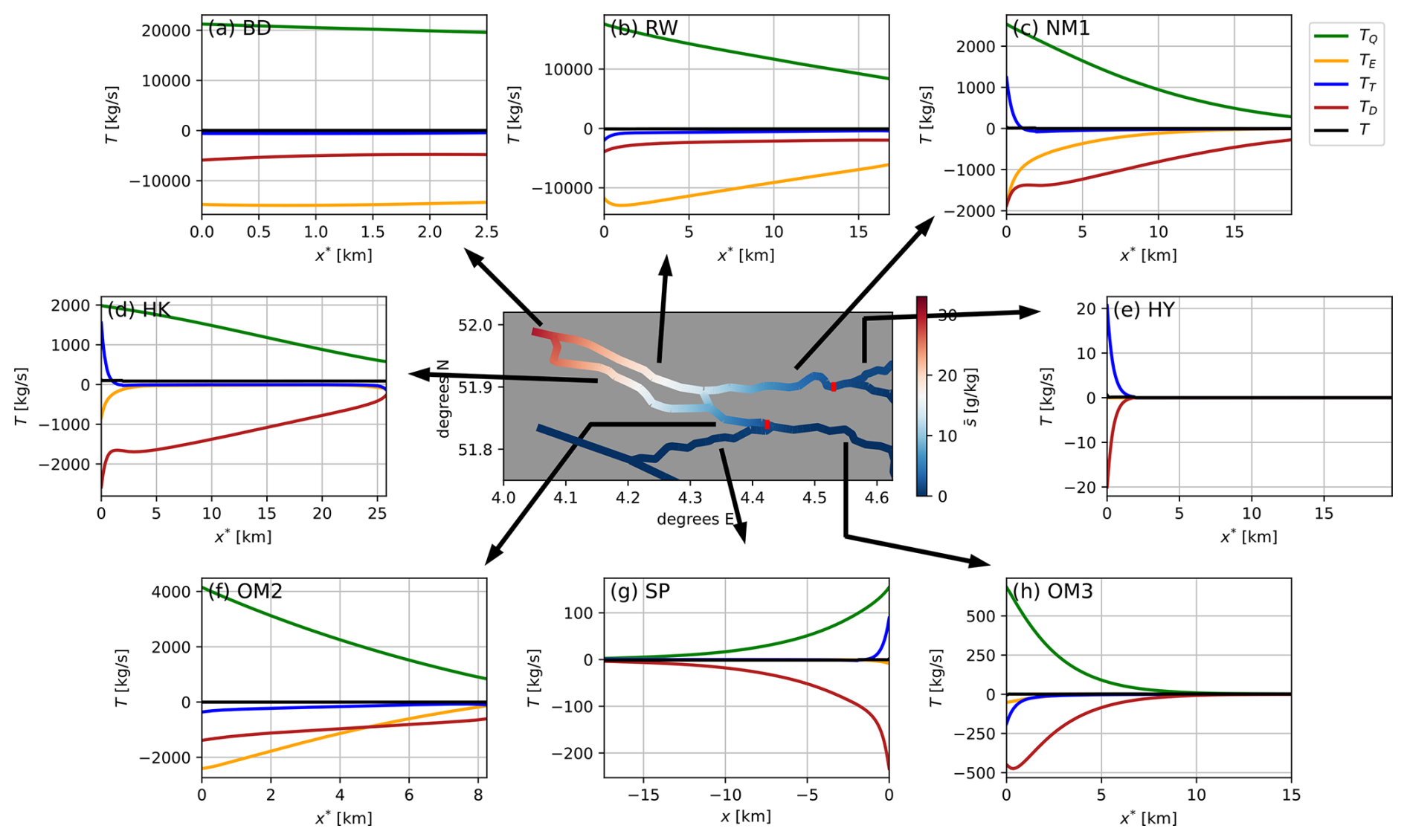
Figure 5 The centre panel shows depth and tidally averaged salinity in the RMD for low-discharge conditions. The red bars in this figure indicate the location of the 2 g kg⁻¹ isohaline. (a–h) The different components of the salt transport in equilibrium, following the decomposition of Eq. (11), versus x or x^*, where we have defined $x^{*}\equiv -x$ for plotting purposes.

3.2 Salt intrusion mechanisms

3.2.1 Method

To quantify the mechanisms of salt transport in an estuarine network (the second research aim), an equilibrium simulation is performed with the calibrated model. To this end, the model is forced with discharges that represent low-discharge conditions, as this is the situation in which salt intrusion is the most relevant. For the Haringvliet sluices and the Hollandse IJssel and Lek rivers, we set the discharge to zero, while for the Waal River, we use Q=650 m³ s⁻¹ and for the Maas River, Q=50 m³ s⁻¹. These values equal approximately the minimum observed discharges in the summer of 2022.

The distribution of net water transport and subtidal salinity in different channels in the RMD is presented in Fig. S2; the associated components of the salt transport in different channels in the RMD for low-discharge conditions are shown in Fig. 5.

3.2.2 Main channels

It turns out that close to the sea boundary (BD, RW), salt transport related to the exchange flow T_E is the most important contribution to the salt transport, while further inland its relative contribution decreases. This spatial pattern is explained by the fact that close to the sea boundary, depth is large, but further inland, the RMD becomes shallower (e.g. H=16 m for BD and RW but H=11 m for NM1 and H=10.2 m for OM3). The strength of the exchange flow $u_{\mathrm{st}}^{\prime }$ scales with H³ (Eq. 3c), and the variable $s_{\mathrm{st}}^{\prime }$, which is mainly generated by this flow, thus decreases when depth decreases (Fig. S3). The salt transport component T_E is the product of those two and therefore strongly depends on depth.

The salt transport component due to horizontal dispersion T_D becomes dominant in most areas where T_E declines (e.g. NM1, SP, OM3). This is because the dependence of T_D on depth is weaker (only through a decrease in the cross-section).

3.2.3 Tidal transport

The component due to tides (T_T) is small in most of the network. To explain this, we compute the phase difference between depth-averaged tidally varying flow and salinity, which is very important to the magnitude of T_T (see Eq. 11). A phase difference of more (less) than 90° is associated with upstream (downstream) salt transport. In our model context, this phase difference is generated by two mechanisms: vertical advection of subtidal salinity within the tidal cycle (Biemond et al., 2024a) and interaction with other channels around junctions. The first mechanism requires the presence of tidally averaged vertical salinity gradients, which are mainly are created by the exchange flow. This gives, for example, a phase difference of about 95° in the RW (Fig. S4), which yields T_T≈500 kg s⁻¹, about 15 times smaller than T_E. Note that a T_T of this strength would be the dominant salt transport in channels further upstream (e.g. OM3). In the channels where exchange flow is weaker, the phase difference that is induced is also smaller, and therefore T_T is a subdominant component of the salt transport except around some junctions. The net salt transport due to vertical variations in the tidally varying flow and salinity is not considered for this explanation because its contribution to salt transport is negligible, as explained in Biemond et al. (2024a).

3.2.4 Transport in the vicinity of junctions

Near junctions such as the SP–OM2–OM3 or the BD–RW–HK, the distortion of the phase difference from 90° increases strongly, for example, around the seaward boundary of the HK, NM1, and HY, where the minimum phase difference is about 60° (Fig. S4). Here, T_T also reverses sign (i.e. it turns seaward) along the salinity gradient. Note that for each junction in only one connected channel is the phase difference below 90°. To illustrate this behaviour, we study the case of the junction of the HY, NM1, and NM2 in detail, but similar reasoning applies to the other junctions. Figure 6 visualises tidal currents and salinity around this junction. Figure 6a shows that ${\stackrel{\mathrm{‾}}{u}}_{\mathrm{ti}}$ in the HY leads the currents in the other two channels by about 1.5 h. The consequences for the salt transport are made clear by studying the different phases of the tide. When the currents in all channels are positive (i.e. the red shaded area and panel 1), relatively fresh water from upstream is transported downstream, and salinity at the junction decreases (Fig. 6b). At some point, the current in the HY will change direction before the currents in the other channels change direction (the blue shaded area and panel 2). In this phase, the HY will receive freshwater from upstream, i.e. from the NM2. After about 1.5 h, currents in the other channels will also change direction (the light blue area and panel 3), and saline water from downstream is imported into the channels. However, when salinity at the junction reaches its maximum value, ${\stackrel{\mathrm{‾}}{u}}_{\mathrm{ti}}$ in the HY has already changed direction (the yellow area and panel 4), and this salinity does not reach the HY. The tidally averaged transport T_T is upstream in the main channels (NM1 and NM2), while it is downstream in the side channel (HY).

3.2.5 Minor channels

The HY (and also the LE) is a special case in the sense that it does not receive discharge from upstream, and therefore T_Q is zero throughout this channel. The absence of discharge, which is the main source of buoyancy, also implies that (tidally averaged) vertical salinity gradients are almost absent: the top–bottom salinity difference is 0.09 g kg⁻¹ at 1 km from the junction in the HY. This implies that T_E is weak (i.e. $\frac{T_{\mathrm{E}}}{T_{\mathrm{D}}}=\mathrm{5}\times {\mathrm{10}}^{-\mathrm{4}}$) at this location.

A similar situation occurs in the HK, which is shallower than its neighbouring channels: it receives less discharge (71 m³ s⁻¹; about 9 times smaller than the RW) and is consequently less stratified, and the channel-averaged contribution of T_E to the upstream salt transport in the HK is only 4 % (Fig. 5d).

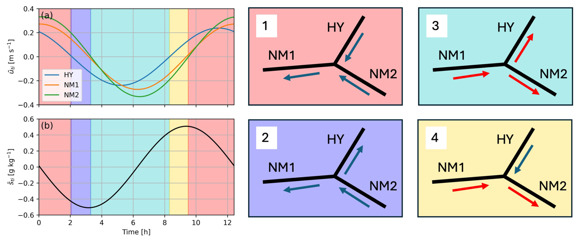
Figure 6 (a) Depth-averaged tidal velocity ${\stackrel{\mathrm{‾}}{u}}_{\mathrm{ti}}$ within a tidal cycle at the junction of the Hollandse IJssel (in blue), Nieuwe Maas 1 (in orange), and Nieuwe Maas 2 (in green). (b) As (a), but for depth-averaged tidal salinity ${\stackrel{\mathrm{‾}}{s}}_{\mathrm{ti}}$. Panels 1–4 show the visualisation of the situation during different phases of the tide. The background colours correspond to the colours of panels (a) and (b). The arrows indicate the direction of the current, and the colour indicates whether the water is relatively fresh (blue) or relatively saline (red).

3.2.6 Overspill

The absolute value of the total salt transport $\left|T\right|$ is 80 kg s⁻¹ in the HK, OM1, and RW, indicating the presence of salt overspill in these channels. Overspill occurs when salt originating from one channel is transported downstream with the subtidal current ${\stackrel{\mathrm{‾}}{u}}_{\mathrm{st}}$ through another channel. In Fig. S2, the direction of this transport is indicated. For the range of values of the parameters investigated in this study, this only occurs in the RW–OM1–HK channel system in the RMD. Under the low-discharge conditions studied here, its contribution to the total salt transport in the HK is 13 %.

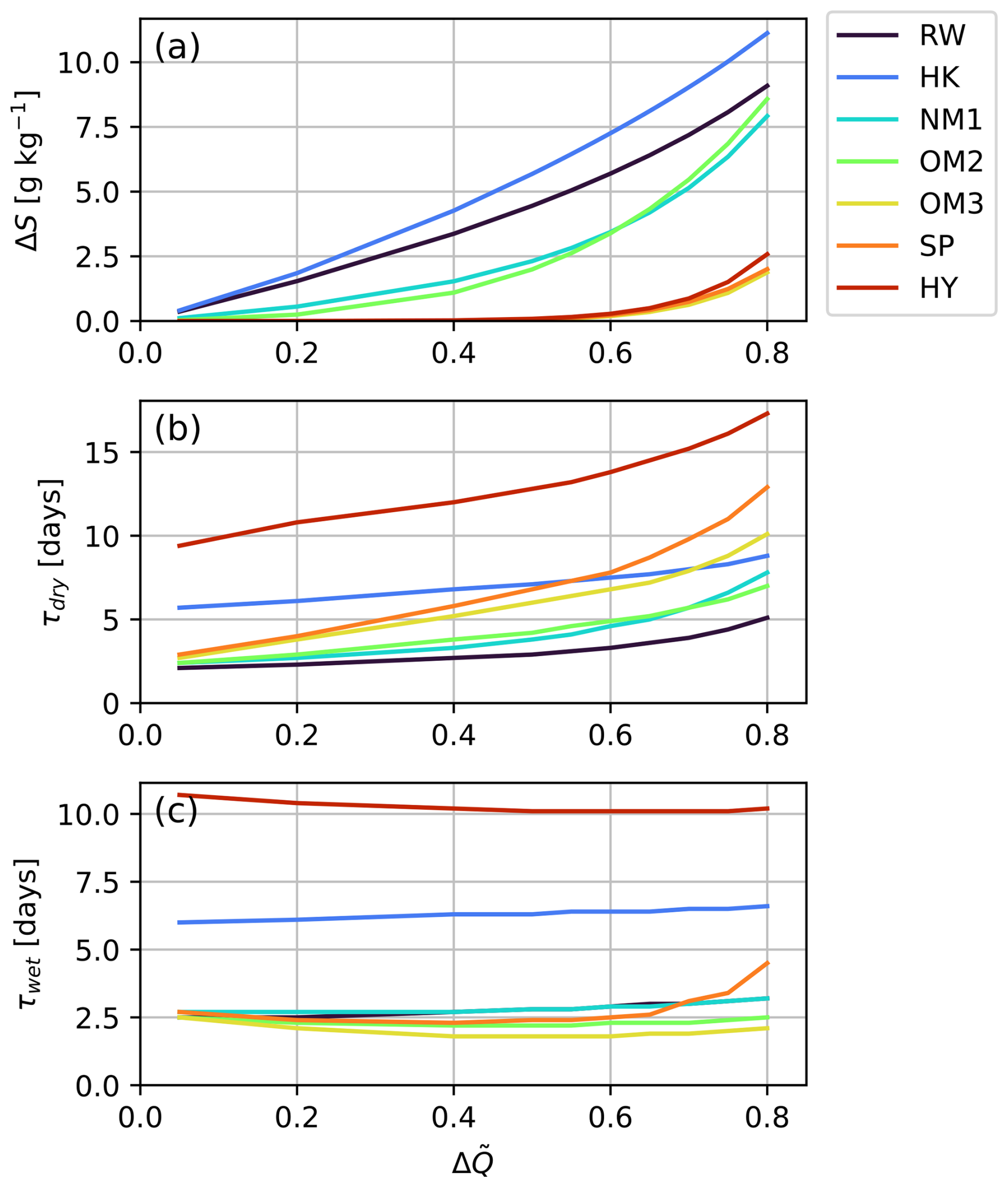
Figure 7 (a) Absolute value of the change in channel-averaged salinity ΔS of different channels as a function of the change in discharge $\mathrm{\Delta }\stackrel{\mathrm{̃}}{Q}=\frac{Q_{\mathrm{ref}}-Q_{\mathrm{dry}}}{Q_{\mathrm{ref}}}$, where Q_ref is the yearly average discharge and Q_dry the decreased discharge. Note that ΔS is independent of the sign of the change in discharge because absolute values are considered. (b) As (a), but for the response time τ_dry due to a decrease in river discharge, i.e. a transition from Q_ref to Q_dry. (c) As (b), but for the response time τ_wet due to an increase in river discharge, i.e. a transition from Q_dry to Q_ref.

3.3 Response to changes in discharge

3.3.1 Method

To examine the response of salinity in the network to changes in discharge (the third research aim), the model is forced with discharge time series that represent the transition from reference discharge conditions to low-discharge conditions and vice versa. For the Haringvliet sluices and the Hollandse IJssel River, discharge is set to zero. In the reference situation, the Lek, Waal, and Maas rivers are forced with their yearly average discharge, which is 490, 1500, and 230 m³ s⁻¹, respectively. To simulate the response to a transition to low-discharge conditions, the reference discharges are multiplied by a factor ranging from 0.95 to 0.2 for the different scenarios. In this way, the fraction of the total discharge received per channel does not change. The simulation is continued until equilibrium has been reached. To simulate the response to an increase in river discharge, discharge is increased from the lowered value to the yearly average values, and again the simulation is continued until equilibrium has been obtained. Note that these simulations do not reproduce the current water distribution in the RMD during a drought because discharge into the three rivers does not change according to the same ratio due to water management and local differences in drought intensity. Moreover, the Haringvliet sluices are opened when the discharge is high, closed for low discharge, and partially opened in between.

To quantify the salinity response to a change in discharge, studies of single-channel estuaries have analysed the evolution of a certain isohaline, typically the 2 g kg⁻¹ isohaline (Chen, 2015; Monismith, 2017). However, in a network this is not generally possible, as isohalines are not bound to a certain channel. Therefore, an alternative measure for the salt intrusion into a channel is used for response times, which is based on the channel-averaged salinity S, defined as $S=\frac{{\int }_V{s}_{\mathrm{st}}\mathrm{d}V}{V}$, where V is the volume of the channel. The response time is then defined as when 90 % of the change in S has occurred (note that S becomes constant after the change in discharge). We indicate the time it takes to respond to a low discharge as τ_dry and the time it takes to respond to a high (i.e. the reference) discharge as τ_wet.

3.3.2 General behaviour

The changes in mean salinity and the response times of individual channels in the RMD after an increase or decrease in the discharge of the Lek, Waal, and Maas rivers are shown in Fig. 7. A larger change in discharge is associated with a larger change in mean salinity, as was expected. The absolute changes in salinity are larger for channels close to the sea (RW, HK) but smaller for channels close to the limit of the salt intrusion (SP, HY, OM3). Regarding response times, τ_dry increases for larger changes in discharge (the τ_dry associated with an 80 % change in discharge is 61 % larger than the τ_dry of a 5 % change for the channels considered in Fig. 7), but τ_wet is not sensitive to the magnitude of the change in discharge (the τ_wet associated with an 80 % change in discharge is only 9 % larger than the τ_wet of a 5 % change for the channels considered in Fig. 7). This implies that τ_dry and τ_wet differ little for small changes in discharge but that τ_dry exceeds τ_wet for larger changes in discharge.

Following Biemond et al. (2022), who also found this result for single-channel estuaries, the explanation is that τ_dry equals the change in salt content, which scales with the change in salinity, divided by salt import due to T_E and T_D, which depend on the salinity gradient during the adjustment. The change in salinity and salinity gradient are in a different manner related to the change in discharge, and therefore τ_dry depends on the change in discharge. On the other hand, τ_wet is mostly determined by the change in salt content divided by the export of salt due to T_Q, which both scale linearly with salinity, and therefore their ratio does not depend on the change in discharge.

The channels closer to the estuary mouth, i.e. those with high salinity (RW, NM1), have a smaller τ_dry than the channels with low salinity (HY, SP). This is because channels with higher salinity also have larger horizontal and vertical salinity gradients (Figs. S3 and S5), which increases the magnitude of the salt import by T_E and T_D.

3.3.3 Minor channels

The HK and HY have larger response times than their neighbouring channels. We focus first on the HK, for which τ_dry is a factor of 2 higher than in the RW, despite the salinity and salinity gradients being comparable. To explain this, we calculate the total change in salt content in this channel, which equals the channel volume V multiplied by the change in its average salinity, ΔS, divided by its salt import in equilibrium at the downstream boundary (${\mathit{\tau }}_{\mathrm{r}}=\frac{V\mathrm{\Delta }S}{T_{\mathrm{E}}+T_{\mathrm{D}}+T_{\mathrm{T}}}$), which is a lower bound of τ_dry. The salt exchange at the upstream boundary is a factor of 6 smaller in this channel (Fig. 5d) and therefore is not taken into account here. We find τ_r=18.4 h for the HK, τ_r=4.0 h for the NM1, and τ_r=3.0 h for the OM2, for comparison. Thus, the ratio of salt exchange with the neighbouring channels to the total change in salt content in the HK is smaller than for neighbouring channels, which is because this channel receives little discharge, and this explains the larger τ_dry. The same reasoning holds for the fact that the τ_wet of this channel is larger than in its neighbours, as in equilibrium the salt import equals the salt export, and therefore the salt export is also relatively small.

3.3.4 Closed channels

In the HY, τ_dry is about a factor of 2 higher than that of the other channels. In channels without net water transport like the HY, equilibrium with the forcing conditions will be reached when the horizontal salinity gradient is zero in the channel interior, i.e. when the salinity at the upstream boundary equals the salinity just outside the boundary layer around the junction. This means that the salt front has to intrude over the full length of the channel, which makes the response time larger than for channels with net water transport. Moreover, only the salt transport component T_D (see Sect. 3.2) imports salt into this channel during the adjustment process, while T_T exports salt around the junction (Fig. 5e). The high τ_dry of the HY and more generally of channels without discharge is thus explained by the fact that salt import by T_E is absent and that salt has to intrude over the full length of the channel.

Figure 7c shows that τ_wet is also high in the HY. This is because there is no discharge through the channel that flushes the salinity (through T_Q). Instead, salt is removed by T_D and T_T. As for the other channels, τ_wet is smaller than τ_dry in the HY, but different mechanisms than in most other channels play a role here. First, T_T has the same sign as T_D in the boundary layer around the junction when salinity in the channel decreases, so salt export during a decrease in salinity is faster than salt import during an increase in salinity. Second, the salinity in the channels that the HY is connected to responds faster to an increase in discharge than to a decrease in discharge (compare τ_wet and τ_dry of NM1).

3.4 Response to changes in depth

3.4.1 Method

Effects of changes to the depth of individual channels on salt intrusion in the major branches (the fourth research aim) are quantified by analysing the output of a set of equilibrium simulations that have the same forcing conditions as the simulation for the second research aim. In each of these simulations, the depth of one of the channels in the network is increased or decreased by 25 %. The impact on the salt intrusion is quantified by means of the distance X₂ from the RW–NM1–OM1 junction to the subtidal 2 g kg⁻¹ isohaline in the Nieuwe Maas (consisting of channels NM1 and NM2) and in the Oude Maas (consisting of channels OM1, OM2, OM3, and OM4), the two major branches of the network. The locations of these isohalines are shown in the centre panel of Fig. 5. These quantities can be converted into the distance to the sea boundary by adding the length of the BD and of the RW, which is 19.3 km in total.

Salt intrusion lengths X₂ of the Oude Maas and Nieuwe Maas for changes in the depth of individual channels are shown in Fig. 8a. In contrast to the simulations for Sect. 3.3, the net water transport distribution changes when the depth changes, and the values for the major branches are presented in Fig. 8b. The responses of the salt intrusion lengths range from no detectable change in X₂ to a maximum change of 12 km. In the following, we will explain the mechanisms that are responsible for the different responses.

3.4.2 Seaward channels

Changes in the depth of the most seaward channels (BD and RW) affect the extent of the salt intrusion (increases when deepening, decreases when shoaling) because upstream salt transport in these channels is dominated by T_E (Fig. 5a), which depends strongly on the local depth (Sect. 3.2). Changing the depth of the RW has a larger effect on X₂ than changing the depth of the BD because the RW is longer.

The magnitude of the change in X₂ due to a decrease +ΔH in depth exceeds the change after an increase −ΔH. Scaling relations between the depth and extent of the salt intrusion in single-channel estuaries (Monismith et al., 2002) predict a scaling with H³ when T_E is the dominant salt import mechanism, which implies that, in contrast to what we find, an increase in depth would result in a larger absolute change in X₂ rather than a decrease.

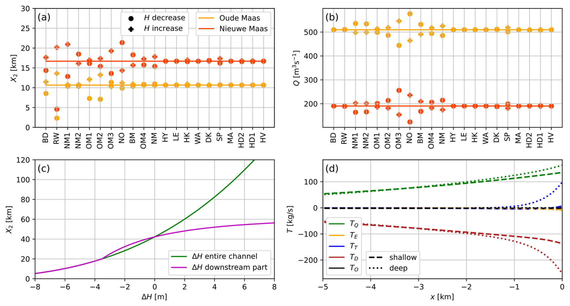
Figure 8 (a) The salt intrusion length X₂, defined as distance from the RW–NM1–OM1 junction to the 2 g kg⁻¹ isohaline in the Oude Maas (yellow) or Nieuwe Maas (red) versus the changes in depth of different channels. The dots indicate a decrease in depth, and the plus markers indicate an increase in depth. The lines indicate X₂ with the current geometry. (b) As (a), but for the net water transport through OM1 (yellow) and NM1 (red). (c) Salt intrusion length X₂ of a single-channel estuary that consists of two segments as a function of change in depth ΔH of the entire estuary (green) or change in depth of the downstream 20 km (purple) around a reference depth of 16 m (the depth of the RW), using Eqs. (D4) and (D5). (d) As Fig. 5g, but for a shallower HD1 (dashed line) or a deeper HD1 (dotted line) and zoomed in on the 5 km of the channel adjacent to the SP–OM2–OM3 junction.

To understand why the scaling is different in a network, a simple model for the RW is constructed, which mimics the RW as a single-channel estuary but with two segments and assumes a balance between T_Q and T_E (the Chatwin, 1976, balance), which are the dominant salt transport components in the RW (Fig. 5b). The details of the model are in Appendix D. In this case, analytical solutions for the salt intrusion length as a function of depth are obtained. Two scenarios are considered: in the first, the depth of the entire channel is changed. In the second, only the depth of the downstream 20 km long segment of the channel is changed. The results are shown in Fig. 8c. When the depth of the entire channel is changed (the green line), an increase in depth has a larger impact than a decrease in depth, which follows from the previously mentioned H³ scaling (Eq. D2). However, when the depth of only the downstream part of the channel is changed (the purple line), a deepening +ΔH has a smaller effect than shoaling −ΔH. This is because when the depth is increased, the salt intrusion length increases, and only a limited part of the salt intrusion experiences a larger depth and the associated increase in salt transport. In the case of shoaling, the salt intrusion length decreases, and a relatively large part of the salt intrusion experiences a smaller depth and the related decrease in salt transport. As the RW and BD are within the range of salt intrusion, increasing their depth has a smaller effect than decreasing their depth.

3.4.3 Main channels

For changes to the depth of channels that are a part of the major branches Oude Maas and Nieuwe Maas, two competing mechanisms play a role. The first is that deepening increases the magnitude of T_E. The second mechanism is that, simultaneously, the net water transport through the branch will increase due to a decrease in friction, causing an increase in T_Q. Because of volume conservation, the magnitude of the change in net water transport is equal to that of the other major branch but with the opposite sign. The change in friction when changing the depth also affects the tidal currents, but the changes in the salt transport component T_T are negligible. The interplay of these mechanisms means that when deepening channels that are part of the major branches and are within the limit of the salt intrusion (i.e. the NM1, OM1, and OM2), salt intrusion increases. This is because locally the magnitude of T_E increases, which dominates the increase in T_Q. In the other major branch, salt intrusion increases as well because net water transport decreases (Fig. 8b). On the other hand, changing the depth of the channels that are part of the major branches but outside the limit of the salt intrusion (NM2, OM3) does not affect T_E directly but only T_Q. This means that an increase in depth decreases salt intrusion into the major branch that the channel is part of and simultaneously increases salt intrusion into the other major branch. Note that the statements in this section are given for deepening. For shoaling, we find the opposite effect. Changes in net water transport also explain the response of channels that are important for the distribution of the Waal River discharge (i.e. the NO, BM, OM4, and NM). The NO in particular has a large effect on salt intrusion into the Nieuwe Maas, as this channel exerts a strong control on the amount of discharge from the Waal River that reaches the Nieuwe Maas. The salt intrusion into the Nieuwe Maas is more sensitive to changes in net water transport than that into the Oude Maas because the net water transport through the Nieuwe Maas is about 2.5 times smaller than that through the Oude Maas (Fig. 8bf).

3.4.4 Other channels

Changes in the depth of the other channels in the RMD (HY in Fig. 8a and all channels to its right) have little impact on X₂ in the Nieuwe Maas and Oude Maas (changes are less than 1 km). There are, however, two cases that have an interesting local effect. The first concerns a change in depth in the HK. In the reference simulation, salt overspill occurs in the HK (T=80 kg s⁻¹), and salt from the Oude Maas is transported seawards through the HK (Figs. 5d and S2). When decreasing its depth, the magnitude of the salt transport due to salt overspill increases (T=540 kg s⁻¹), but when increasing the depth, the sign of T reverses, and the HK becomes a source of salt for the Oude Maas ($T=-\mathrm{250}$ kg s⁻¹). The consequence of this change in salt transport for the salt intrusion length is only a few hundred metres because this salt transport is relatively weak compared to the amount of salt transported from the RW into the Oude Maas. The second interesting behaviour concerns an increase or decrease in the depth of the HD1. These have little impact on X₂ in the Oude Maas and Nieuwe Maas but affect the extent of the salt intrusion into the SP. The distance of the 0.5 g kg⁻¹ isohaline in the SP from the junction with the OM2 and OM3 is 6.3, 5.2, and 4.8 km for the shallow, reference, and deep HD1, respectively, so shoaling the HD1 affects salt intrusion more than deepening. To understand this, we calculate the change in salt transport components T_Q and T_T (the flow associated with these components of the salt transport directly changes in the SP due to a change in the depth of the HD1). The difference in T_Q is about 30 kg s⁻¹ between the shallow and deep HD1. Figure 5g shows that for the reference depth, T_T in the SP close to its seaward boundary is positive; in other words, the salt transport due to tidal currents is directed towards the SP–OM2–OM3 junction. Figure 8d shows that this situation persists for a deep HD1, but when decreasing the depth of HD1, the magnitude of T_T decreases due to a shift in phases of the tidal currents of the different channels around this junction. The difference in T_T at the junction is about 90 kg s⁻¹, 3 times larger than the change in T_Q, indicating that the change in tidal currents dominates the change in salt intrusion into the SP when deepening the HD1.

4 Discussion

4.1 Comparison with observations

When our idealised network model is applied to the RMD and calibrated against observations, it has a Nash–Sutcliffe efficiency of 0.67. This indicates that the model performance with regard to simulating salinity is satisfactory despite the fact that the descriptions of the physics, forcing conditions, and bathymetry are rather simple. The gradient descent algorithm to find optimal values of the calibration coefficients is crucial to obtain satisfactory model performance.

The effects of the non-resolved aspects of the salinity dynamics on the salt transport are via the calibration mostly projected onto horizontal salt dispersion. A value of $K_{\mathrm{h},\mathrm{st}}=\mathrm{275}$ m² s⁻¹ is found, and with this value T_D, the tidal dispersion, is the dominant salt transport component in parts of the RMD, in particular around the limit of the salt intrusion. However, since most of the observation points are in the larger channels of the network, this value of tidal dispersion mainly represents the unresolved salt transport in these channels. A hint that in the smaller channels of the network this constant value is too large follows from the described difference in model–data agreement between points a₃ and a₄ (see Sect. 3.1). Model extensions that could possibly resolve this disagreement are discussed in Sect. 4.4.

4.2 Changes in discharge

We found that response times vary between the channels and attributed this to differences in the salinity gradients, the volume/transport ratios of the channels, and the presence of net water transport in the channels. Observations show that response times to changes in forcing are 10–14 d for the HY (Laan et al., 2021), in line with what we find. In another estuarine network, the Po Delta, differences in response times between the channels are minor (Bellafiore et al., 2021, Fig. 5a). This is because in that delta, all channels receive a considerable fraction of the river discharge, and differences in channel depth are also relatively small compared to those in the RMD. Therefore, dynamics of features such as the side branches, like the HY in the RMD, do not play a role in the Po Delta. Certain aspects of the theory of the response of single-channel estuaries to changes in river discharge can be transferred to estuarine networks, for example, the reason for the asymmetry in the response to an increase or decrease in discharge. However, a direct comparison with single-channel estuaries is hindered by factors such as differences in definitions of response times, for reasons that were explained in Sect. 3.3.

4.3 Changes in depth

We showed that in a network, the response of the salt intrusion to changes in depth is sensitive to which channel is changed. Salt intrusion can decrease locally when parts of an estuarine network are deepened due to a redistribution of the river water. This is different for single-channel estuaries, for which it is found that salt intrusion increases when the depth increases (Ralston and Geyer, 2019; Siles-Ajamil et al., 2019; Kolb et al., 2022). Liu et al. (2019) also reported effects on salt intrusion when discharge changes upstream in a network (the Pearl River Delta) due to alterations in the depth. For the Yangtze Estuary, Zhu et al. (2006) reported that salt intrusion increased in multiple channels when the depth of one the channels was increased, in line with what we find for the RMD. Huismans and Plieger (2019) showed, using a 3D model of the RMD, that a shallower Oude Maas leads to a decrease in salt intrusion in the Nieuwe Maas as well as in the Oude Maas. However, when winds and storm surges are accounted for, a more complicated response to changes in depth occurs. They hypothesised that changes in phases of the currents around the junction could be important to the response to changes in depth; we showed that they indeed can play an important role. For a deepening of the RW, Laan et al. (2023) found that salt intrusion in the entire RMD changes, but when deepening the LE, the effect remains local, which is again in line with what we find.

4.4 Future research

As explained in Sect. 2.1, certain model aspects are highly simplified, which limits the range of simulated salt dynamics in estuarine networks. The fact that only one tidal constituent is considered and that the balances for tidal flow and salinity are simplified implies that not all processes contributing to salt transport by the tidal current are included. Also, the vertical eddy viscosity, vertical eddy diffusivity, and horizontal dispersion coefficients are assumed to be constant in space and time in our model. Varying these coefficients with bathymetry would lead to a different response to changes in bathymetry.

We present here recommendations on how to improve these model aspects, to gain more insight into the salt dynamics in estuarine networks. To improve the description of tidal salt transport, additional mechanisms that generate a phase difference between tidal currents and salinity, for example, multiple tidal constituents (externally forced and internally generated), lateral effects (Scully and Geyer, 2012), or tidal trapping in side embayments (Okubo, 1973; Geyer and Signell, 1992; MacVean and Stacey, 2011), could be included. However, finding a suitable description of these processes in the simplified model may not be straightforward. Next, more realistic parametrisations of vertical eddy viscosity, vertical eddy diffusivity, and horizontal dispersion coefficients could be employed. Other studies argue that the vertical eddy viscosity and vertical eddy diffusivity coefficients increase with the strength of the tidal currents and with increasing depth of the channels and decrease with increasing stratification (Monismith et al., 2002; MacCready, 2007). These effects could be included to improve the description of the turbulence closure of the model. For the horizontal dispersion coefficient, different parametrisations are proposed (Banas et al., 2004; MacCready, 2007; Aristizábal and Chant, 2015). However, the use of these formulations in our model is hindered by the fact that we explicitly resolve part of the salt transport by the tidal current.

Another direction for future research is the inclusion of additional forcing conditions, for example, water level fluctuations at subtidal and intratidal timescales at the sea boundary (Kranenburg et al., 2022) and water extractions, which are on the order of 100 m³ s⁻¹ (Huismans et al., 2024), about one-seventh of the total discharge in dry conditions.

5 Conclusions

The main findings, based on simulations with our idealised, partly analytical, 2DV model of an estuarine network, are the following:

1. The network model, when calibrated, has satisfactory agreement with observations, despite missing potentially important aspects of the salinity dynamics. The reason for this is that the salt transport associated with these aspects projects well onto the calibrated processes, especially onto the horizontal salt dispersion. A consequence is that local variations in the salt transport due to tidal currents are only crudely resolved.

2. Salt transport components related to different mechanisms vary in relative importance within a network due to differences in water depth, discharge, phases of the tidal currents, and characteristics of the salt field itself. In the deeper channels of the RMD, upstream salt transport by exchange flow is dominant, but in the shallower parts, tidal dispersion takes over. Salt transport by tidal currents can be directed seawards around a junction when the currents of the different channels are out of phase.

3. Channels closer to the estuary mouth respond faster to changes in discharge than those further upstream. The response to an increase in discharge is faster than the response to a decrease, in agreement with theory of single-channel estuaries. Channels that receive little discharge have large response times, especially when the net water transport is zero.

4. The impact of changes in the depth of an individual channel in a network on the extent of salt intrusion into the major branches depends on where the change takes place. The impact is determined by the direct, local effect on factors such as the strength of the exchange flow and the interaction with other channels, which is related to changes in the distribution of discharge and tidal currents. Scaling relationships developed for single-channel estuaries are found to be invalid for depth changes in an estuarine network. Salt intrusion into a channel with lower discharge is more sensitive to changes in depth than into a channel with higher discharge. The phase differences in tidal currents around a junction are sensitive to changes in the depth, and this sensitivity can be the cause of changes in salt intrusion when the depth of a channel in another part of the network is changed.

Appendix A: Geometry of the Rhine–Meuse Delta

Table A1 Geometry of the Rhine–Meuse Delta used in the model. The abbreviations correspond to Fig. 2. The widths at the boundaries of the channels are provided here; the widths in the interior are computed using Eq. 1.

Appendix B: Conditions at internal boundaries

There are two types of internal boundaries in the model: connections between segments and junctions. The conditions below are given for junctions. For connections between segments, the same conditions apply, but only two channels are considered. The conditions for hydrodynamics at the internal boundaries read

$$\begin{array}{}\text{(B1)}& \begin{array}{rl}& \sum _{p=\mathrm{1}}^{\mathrm{3}}{b}_p{H}_p{\stackrel{\mathrm{‾}}{u}}_{\mathrm{st},p}=\mathrm{0},{\mathit{\eta }}_{\mathrm{st},\mathrm{1}}={\mathit{\eta }}_{\mathrm{st},\mathrm{2}}={\mathit{\eta }}_{\mathrm{st},\mathrm{3}},\\ & \sum _{p=\mathrm{1}}^{\mathrm{3}}{b}_p{H}_p{\stackrel{\mathrm{‾}}{u}}_{\mathrm{ti},p}=\mathrm{0},{\mathit{\eta }}_{\mathrm{ti},\mathrm{1}}={\mathit{\eta }}_{\mathrm{ti},\mathrm{2}}={\mathit{\eta }}_{\mathrm{ti},\mathrm{3}},\end{array}\end{array}$$

where subscripts 1, 2, and 3 are indices of the channels that are connected to the junction. Regarding salinity, continuity of salt transport and salinity is used at every vertical level, which reads

$$\begin{array}{}\text{(B2a)}& {\displaystyle }\sum _{p=\mathrm{1}}^{\mathrm{3}}{T}_p=\mathrm{0},{\stackrel{\mathrm{‾}}{s}}_{\mathrm{st},\mathrm{1}}={\stackrel{\mathrm{‾}}{s}}_{\mathrm{st},\mathrm{2}}={\stackrel{\mathrm{‾}}{s}}_{\mathrm{st},\mathrm{3}},\text{(B2b)}& {\displaystyle }\begin{array}{rl}& \sum _{p=\mathrm{1}}^{\mathrm{3}}{b}_p{H}_p(u_{\mathrm{st},p}^{\prime }{s}_{\mathrm{st},p}^{\prime }-\stackrel{\mathrm{‾}}{u_{\mathrm{st},p}^{\prime }{s}_{\mathrm{st},p}^{\prime }}\\ & +{\left(u_{\mathrm{ti},p}^{\prime }{s}_{\mathrm{ti},p}^{\prime }-\stackrel{\mathrm{‾}}{u_{\mathrm{ti},p}^{\prime }{s}_{\mathrm{ti},p}^{\prime }}\right)}_{\mathrm{st}}-K_{\mathrm{h},\mathrm{st}}{\displaystyle \frac{\partial s_{\mathrm{st},p}^{\prime }}{\partial x}})=\mathrm{0},\\ & s_{\mathrm{st},\mathrm{1}}^{\prime }=s_{\mathrm{st},\mathrm{2}}^{\prime }=s_{\mathrm{st},\mathrm{3}}^{\prime },\end{array}\text{(B2c)}& {\displaystyle }\begin{array}{rl}& \sum _{p=\mathrm{1}}^{\mathrm{3}}{b}_p{H}_p\left(u_{\mathrm{ti},p}{s}_{\mathrm{ti},p}+u_{\mathrm{ti},p}{s}_{\mathrm{ti},p}-K_{\mathrm{h},\mathrm{ti}}{\displaystyle \frac{\partial s_{\mathrm{ti},p}}{\partial x}}\right)=\mathrm{0},\\ & s_{\mathrm{ti},\mathrm{1}}=s_{\mathrm{ti},\mathrm{2}}=s_{\mathrm{ti},\mathrm{3}}.\end{array}\end{array}$$

Note that the conditions for the vertically varying quantities are evaluated at sigma levels (i.e. at $\stackrel{\mathrm{̃}}{z}=\frac{z}{H}=$ constant) when the channels have non-equal depths.

Appendix C: Boundary layer correction for salinity at junctions

The first-order equation for tidally varying salinity s_ti reads (Biemond et al., 2024a)

$$\begin{array}{}\text{(C1)}& {\displaystyle \frac{\partial s_{\mathrm{ti}}}{\partial t}}+u_{\mathrm{ti}}{\displaystyle \frac{\partial {\stackrel{\mathrm{‾}}{s}}_{\mathrm{st}}}{\partial x}}+w_{\mathrm{ti}}{\displaystyle \frac{\partial s_{\mathrm{st}}^{\prime }}{\partial z}}={\displaystyle \frac{\partial }{\partial x}}\left(K_{\mathrm{h},\mathrm{ti}}{\displaystyle \frac{\partial s_{\mathrm{ti}}}{\partial x}}\right)+{\displaystyle \frac{\partial }{\partial z}}\left(K_{\mathrm{v},\mathrm{ti}}{\displaystyle \frac{\partial s_{\mathrm{ti}}}{\partial z}}\right),\end{array}$$

in which t is time; u_ti and w_ti are the horizontal and vertical components of the tidal current, respectively; ${\stackrel{\mathrm{‾}}{s}}_{\mathrm{st}}$ is the depth and tidally averaged salinity; $s_{\mathrm{st}}^{\prime }$ is the vertical distortion from the tidally averaged salinity; and K_h,ti and K_v,ti are the horizontal dispersion coefficient and vertical eddy diffusivity coefficient acting on the tidal salinity, respectively. The boundary conditions are no flux at the bottom and surface and Eq. (B2c) for the horizontal boundaries (junctions). The horizontal dispersion term is included in Eq. (C1). In Wei et al. (2016) and Biemond et al. (2024a), it was argued that this term is small with respect to the other terms in this equation. We argue here that horizontal dispersion is important in the neighbourhood of junctions, as tidal currents are observed to be more turbulent close to junctions (Corlett and Geyer, 2020), which increases the magnitude of dispersion. Moreover, when horizontal dispersion is excluded, Eq. (C1) does not contain horizontal derivatives of s_ti, which implies that no horizontal boundary conditions can be applied, and therefore the continuity of salinity at the junctions cannot be imposed.

To develop a set of equations that takes horizontal dispersion into account around the junctions, we scale Eq. (C1) by defining

$$\begin{array}{}\text{(C2)}& \begin{array}{rl}& t={\mathit{\omega }}^{-\mathrm{1}}\stackrel{\mathrm{̃}}{t},x=L\stackrel{\mathrm{̃}}{x},z=H\stackrel{\mathrm{̃}}{z},u_{\mathrm{ti}}=U{\stackrel{\mathrm{̃}}{u}}_{\mathrm{ti}},\\ & w_{\mathrm{ti}}=H\mathit{\omega }{\stackrel{\mathrm{̃}}{w}}_{\mathrm{ti}},s_{\mathrm{st}}=S_{\mathrm{st}}{\stackrel{\mathrm{̃}}{s}}_{\mathrm{st}},s_{\mathrm{ti}}={\displaystyle \frac{U{S}_{\mathrm{st}}}{\mathit{\omega }L}}{\stackrel{\mathrm{̃}}{s}}_{\mathrm{ti}}.\end{array}\end{array}$$

In these expressions, ω is the frequency of the tide, L is the horizontal length scale on which s_ti varies (when not being affected by junctions), U is the magnitude of the tidal current, and S_st is a typical scale for the subtidal salinity. The last condition follows from $\frac{\partial s_{\mathrm{ti}}}{\partial t}\approx u_{\mathrm{ti}}\frac{\partial s_{\mathrm{st}}}{\partial x}$ (Biemond et al., 2024a). This yields, after dropping the tildes,

$$\begin{array}{}\text{(C3)}& {\displaystyle \frac{\partial s_{\mathrm{ti}}}{\partial t}}+u_{\mathrm{ti}}{\displaystyle \frac{\partial {\stackrel{\mathrm{‾}}{s}}_{\mathrm{st}}}{\partial x}}+{\mathit{\chi }}_{\mathrm{1}}{w}_{\mathrm{ti}}{\displaystyle \frac{\partial s_{\mathrm{st}}^{\prime }}{\partial z}}=\mathit{\epsilon }{\displaystyle \frac{{\partial }^{\mathrm{2}}{s}_{\mathrm{ti}}}{\partial x^{\mathrm{2}}}}+{\mathit{\chi }}_{\mathrm{2}}{\displaystyle \frac{{\partial }^{\mathrm{2}}{s}_{\mathrm{ti}}}{\partial z^{\mathrm{2}}}},\end{array}$$

with ${\mathit{\chi }}_{\mathrm{1}}=\frac{L\mathit{\omega }}{U}$, ${\mathit{\chi }}_{\mathrm{2}}=\frac{K_{\mathrm{v}}}{\mathit{\omega }{H}^{\mathrm{2}}}$, and $\mathit{\epsilon }=\frac{K_{\mathrm{h}}}{\mathit{\omega }{L}^{\mathrm{2}}}$. We write tidally varying salinity as $s_{\mathrm{ti}}=\mathrm{\Re }\left[{\widehat{s}}_{\mathrm{ti}}\exp (-i\mathit{\omega }t)+c.c.\right]$ (see Sect. 2.3) and find the equation

$$\begin{array}{}\text{(C4)}& {\mathit{\chi }}_{\mathrm{2}}{\displaystyle \frac{{\partial }^{\mathrm{2}}{\widehat{s}}_{\mathrm{ti}}}{\partial z^{\mathrm{2}}}}+i{\widehat{s}}_{\mathrm{ti}}+\mathit{\epsilon }{\displaystyle \frac{{\partial }^{\mathrm{2}}{\widehat{s}}_{\mathrm{ti}}}{\partial x^{\mathrm{2}}}}={\widehat{u}}_{\mathrm{ti}}{\displaystyle \frac{\partial {\stackrel{\mathrm{‾}}{s}}_{\mathrm{st}}}{\partial x}}+{\mathit{\chi }}_{\mathrm{1}}{\widehat{w}}_{\mathrm{ti}}{\displaystyle \frac{\partial s_{\mathrm{st}}^{\prime }}{\partial z}}.\end{array}$$

When choosing typical scales for an estuary (H=10 m, L=10 km, U=1 m s⁻¹, $K_{\mathrm{h},\mathrm{ti}}=\mathrm{25}$ m s⁻², $K_{\mathrm{v},\mathrm{ti}}=\mathrm{0.01}$ m s⁻², and $\mathit{\omega }=\mathrm{1.4}\times {\mathrm{10}}^{-\mathrm{4}}$ s⁻¹), it is found that χ₁ and χ₂ are on the same order (1), and ε is a factor of 10³ smaller. This defines a singular perturbation problem, which is solved using standard techniques (see e.g. Eckhaus, 2011).

To construct the regular solution, we write

$$\begin{array}{}\text{(C5)}& {\widehat{s}}_{\mathrm{ti},\mathrm{reg}}=\sum _{n=\mathrm{0}}^{\mathrm{\infty }}{\mathit{\epsilon }}^n{\mathit{\varphi }}_n.\end{array}$$

Inserting this into Eq. (C4) and collecting the first-order terms give Eq. (10), as is expected, which is valid outside the neighbourhood of the junctions. Close to the junctions, we look for a correction to this equation resulting from the horizontal dispersion. We write $\mathit{\psi }={\widehat{s}}_{\mathrm{ti}}-{\widehat{s}}_{\mathrm{ti},\mathrm{reg}}$ and substitute this, which yields

$$\begin{array}{}\text{(C6)}& \begin{array}{rl}{\mathit{\chi }}_{\mathrm{2}}{\displaystyle \frac{{\partial }^{\mathrm{2}}\mathit{\psi }}{\partial z^{\mathrm{2}}}}& +i\mathit{\psi }+\mathit{\epsilon }{\displaystyle \frac{{\partial }^{\mathrm{2}}\mathit{\psi }}{\partial x^{\mathrm{2}}}}=-{\mathit{\chi }}_{\mathrm{2}}{\displaystyle \frac{{\partial }^{\mathrm{2}}{\widehat{s}}_{\mathrm{ti},\mathrm{reg}}}{\partial z^{\mathrm{2}}}}-i{\widehat{s}}_{\mathrm{ti},\mathrm{reg}}\\ & -\mathit{\epsilon }{\displaystyle \frac{{\partial }^{\mathrm{2}}{\widehat{s}}_{\mathrm{ti},\mathrm{reg}}}{\partial x^{\mathrm{2}}}}+u_{\mathrm{ti}}{\displaystyle \frac{\partial {\stackrel{\mathrm{‾}}{s}}_{\mathrm{st}}}{\partial x}}+{\mathit{\chi }}_{\mathrm{1}}{w}_{\mathrm{ti}}{\displaystyle \frac{\partial s_{\mathrm{st}}^{\prime }}{\partial z}}.\end{array}\end{array}$$

We perform an expansion for the perturbation, i.e. $\mathit{\psi }={\sum }_{n=\mathrm{0}}^{\mathrm{\infty }}{\mathit{\epsilon }}^n{\mathit{\psi }}_n$. The first-order solution then reads

$$\begin{array}{}\text{(C7)}& {\mathit{\chi }}_{\mathrm{2}}{\displaystyle \frac{{\partial }^{\mathrm{2}}{\mathit{\psi }}_{\mathrm{0}}}{\partial z^{\mathrm{2}}}}+i{\mathit{\psi }}_{\mathrm{0}}+\mathit{\epsilon }{\displaystyle \frac{{\partial }^{\mathrm{2}}{\mathit{\psi }}_{\mathrm{0}}}{\partial x^{\mathrm{2}}}}=\mathrm{0}.\end{array}$$

Now a boundary layer coordinate ζ is introduced; i.e. we write ψ₀=B(z)e^ζ, with $\mathit{\zeta }=\pm \frac{x}{{\mathit{\epsilon }}^{\mathit{\nu }}}$. It follows that $\mathit{\nu }=\frac{\mathrm{1}}{\mathrm{2}}$ when the horizontal dispersion term is of equal magnitude to the other terms in Eq. (C7). Substitution of this gives the following equation for B(z):

$$\begin{array}{}\text{(C8)}& {\mathit{\chi }}_{\mathrm{2}}{\displaystyle \frac{d^{\mathrm{2}}B}{\mathrm{d}{z}^{\mathrm{2}}}}+iB+B=\mathrm{0}.\end{array}$$

The no-flux boundary conditions at the bottom and surface apply to this equation. This is a homogenous problem, which has the solution

$$\begin{array}{}\text{(C9)}& B\left(z\right)=\sum _{m=\mathrm{0}}^{\mathrm{\infty }}{B}_m\cos \left(m\mathit{\pi }{\displaystyle \frac{z}{H}}\right).\end{array}$$

The values of B_m follow from the horizontal boundary conditions associated with the junction (Eq. B2c). With this, we have a solution for tidally varying salinity in the neighbourhood of the junctions (the extent of this region is determined by ε^½), which accounts for increased dispersion around the junctions and obeys the horizontal boundary conditions. We set $K_{\mathrm{h},\mathrm{ti}}=\mathrm{25}$ m² s⁻¹; sensitivity tests indicate that the model skill is insensitive to this value.

Appendix D: Derivation of the dependence of salt intrusion on the sign of the change in depth

To explain why an increase in depth of the Rotterdam Waterway (RW) has a smaller effect on salt intrusion in the Nieuwe and Oude Maas than a decrease, we develop a set of equations to study the differences between changing the depth of the downstream part of a channel versus the depth of the entire channel.

Figure D1 A sketch of the domain used in Appendix D.

Suppose that we have a single-channel estuary with constant width in equilibrium, where the salt import is governed by exchange flow, as in the RW. In that case, the terms T_Q and T_E in Eq. (11) balance each other. If we furthermore assume that stratification is the result of a balance between advection of ${\stackrel{\mathrm{‾}}{s}}_{\mathrm{st}}$ by the depth-dependent part of the subtidal current and vertical eddy diffusion (Pritchard, 1954), the following equation for depth-averaged subtidal salinity ${\stackrel{\mathrm{‾}}{s}}_{\mathrm{st}}$ holds (Chatwin, 1976):

$$\begin{array}{}\text{(D1)}& {\displaystyle \frac{Q}{bH}}{\stackrel{\mathrm{‾}}{s}}_{\mathrm{st}}={\displaystyle \frac{\mathrm{0.112}}{{\mathrm{48}}^{\mathrm{2}}}}{\displaystyle \frac{g^{\mathrm{2}}{\mathit{\beta }}^{\mathrm{2}}{H}^{\mathrm{8}}}{A_{\mathrm{v},\mathrm{st}}^{\mathrm{2}}{K}_{\mathrm{v},\mathrm{st}}}}{\left({\displaystyle \frac{\partial {\stackrel{\mathrm{‾}}{s}}_{\mathrm{st}}}{\partial x}}\right)}^{\mathrm{3}}.\end{array}$$

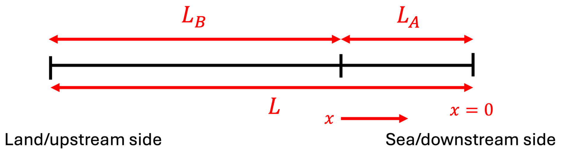
The domain is shown in Fig. D1, and the associated boundary condition is ${\stackrel{\mathrm{‾}}{s}}_{\mathrm{st}}=s_{\mathrm{oc}}$ at x=0.

In a single-channel estuary with length L and constant width, this equation has an analytical solution for salinity, which reads

$$\begin{array}{}\text{(D2)}& \begin{array}{rl}& {\stackrel{\mathrm{‾}}{s}}_{\mathrm{st}}=s_{\mathrm{sc}}{\left({\left({\displaystyle \frac{s_{\mathrm{oc}}}{s_{\mathrm{sc}}}}\right)}^{\frac{\mathrm{2}}{\mathrm{3}}}+{\displaystyle \frac{\mathrm{2}}{\mathrm{3}}}{\displaystyle \frac{x}{L_{\mathrm{e}}}}\right)}^{\frac{\mathrm{3}}{\mathrm{2}}}\text{with}\\ & L_{\mathrm{e}}={\left({\displaystyle \frac{\mathrm{0.112}}{{\mathrm{48}}^{\mathrm{2}}}}{\displaystyle \frac{bH}{Q}}{\displaystyle \frac{g^{\mathrm{2}}{\mathit{\beta }}^{\mathrm{2}}{s}_{\mathrm{sc}}^{\mathrm{2}}{H}^{\mathrm{8}}}{A_{\mathrm{v},\mathrm{st}}^{\mathrm{2}}{K}_{\mathrm{v},\mathrm{st}}}}\right)}^{\frac{\mathrm{1}}{\mathrm{3}}},\end{array}\end{array}$$

where we have introduced the salinity scale s_sc. To be able to change the depth of the downstream part of the channel separately, the single-channel estuary is divided into two segments with lengths L_A and L_B (see Fig. D1). In these segments, Eq. (D2) with $L_{\mathrm{e}}\to L_{\mathrm{e},\mathrm{A}}$, the value of L_e in domain A, is valid for segment A, and for segment B we have

$$\begin{array}{}\text{(D3)}& {\stackrel{\mathrm{‾}}{s}}_{\mathrm{st}}=s_{\mathrm{sc}}{\left({\left({\displaystyle \frac{s_{\mathrm{oc}}}{s_{\mathrm{sc}}}}\right)}^{\frac{\mathrm{2}}{\mathrm{3}}}-{\displaystyle \frac{\mathrm{2}}{\mathrm{3}}}{\displaystyle \frac{L_{\mathrm{A}}}{L_{\mathrm{e},\mathrm{A}}}}+{\displaystyle \frac{\mathrm{2}}{\mathrm{3}}}{\displaystyle \frac{(x+L_{\mathrm{A}})}{L_{\mathrm{e},\mathrm{B}}}}\right)}^{\frac{\mathrm{3}}{\mathrm{2}}},\end{array}$$

where we have used the continuity of salinity at the segment boundary (see Eq. B2a). Note that the values for L_e,A and L_e,B are different when the depths of the segments differ. From these expressions, we can find the position of a certain isohaline X₂ where salinity equals s_tres=2 g kg⁻¹. This yields, for a single-segment estuary,

$$\begin{array}{}\text{(D4)}& X_{\mathrm{2}}={\displaystyle \frac{\mathrm{3}}{\mathrm{2}}}{L}_{\mathrm{e}}\left({\left({\displaystyle \frac{s_{\mathrm{oc}}}{s_{\mathrm{sc}}}}\right)}^{\frac{\mathrm{2}}{\mathrm{3}}}-{\left({\displaystyle \frac{s_{\mathrm{tres}}}{s_{\mathrm{sc}}}}\right)}^{\frac{\mathrm{2}}{\mathrm{3}}}\right).\end{array}$$

For an estuary consisting of two segments, Eq. (D4) (with $L_{\mathrm{e}}\to L_{\mathrm{e},\mathrm{A}}$) is also valid if the salt intrusion is confined to the first segment. In the case that X₂ is located in segment B, it follows that

$$\begin{array}{}\text{(D5)}& X_{\mathrm{2}}=L_{\mathrm{A}}+{\displaystyle \frac{\mathrm{3}}{\mathrm{2}}}{L}_{\mathrm{e},\mathrm{B}}\left({\left({\displaystyle \frac{s_{\mathrm{oc}}}{s_{\mathrm{sc}}}}\right)}^{\frac{\mathrm{2}}{\mathrm{3}}}-{\left({\displaystyle \frac{s_{\mathrm{tres}}}{s_{\mathrm{sc}}}}\right)}^{\frac{\mathrm{2}}{\mathrm{3}}}-{\displaystyle \frac{\mathrm{2}}{\mathrm{3}}}{\displaystyle \frac{L_{\mathrm{A}}}{L_{\mathrm{e},\mathrm{A}}}}\right).\end{array}$$

These expressions allow us to study the effect of changes in the depth of the entire channel and changes in the depth of only the downstream segment.