An Atlantic-wide assessment of marine heatwaves beyond the surface in an eddy-rich ocean model

Periods of prolonged anomalously high temperatures in the ocean, known as marine heatwaves (MHWs), can have devastating effects on ecosystems. Although MHWs are extensively studied in the near-surface ocean, little is known about MHWs at depth. As continuous observations in space and time are very sparse away from the surface, basin-wide studies on MHWs at depth have to rely on models. This introduces additional challenges due to the long adjustment timescale of the deep ocean, resulting in long-term drift following the model's initialization. This unrealistic model drift dominates the MHW statistics below approximately 100 m when a fixed baseline is used. As a result, MHW studies at depth require a long model spin-up or have to apply a detrended baseline removing temperature trends. Based on a comparison of two model configurations with eddy-permitting and eddy-rich horizontal resolution, we show that the representation of mesoscale dynamics leads to pronounced differences in the characteristics of MHWs, in particular along the boundaries and along pathways of highly variable currents. Although a high horizontal resolution of the model is important, MHW statistics can be calculated on a coarser grid, which largely decreases the amount of data that needs to be processed. Our results highlight the importance of horizontal and vertical heat transport within the ocean to sub-surface, but also near-surface, MHWs. By investigating the vertical coherence of MHWs in an example region – here, the Cabo Verde archipelago – we show that MHWs are coherent over layers of a few hundred to 1000 m thickness, independent of the baseline used. These ranges are closely related to the vertical structure of the temperature field.

1 Introduction

Marine heatwaves (MHWs) are defined as prolonged periods of anomalously high temperature in the ocean (Hobday et al., 2016). As they can have devastating impacts on marine ecosystems, they have become a major focus of research over the last decade (Smale et al., 2019; Smith et al., 2023). Several recent studies have shown that MHWs are also connected to a range of physical impacts. Berthou et al. (2024), for example, connected the 2023 MHW in the eastern Atlantic to higher land temperatures and increased precipitation probability in the UK, and Radfar et al. (2024) showed that MHWs can influence the development of hurricanes. Furthermore, the study of Krüger et al. (2023) suggests that anomalously high ocean temperatures in the North Atlantic might reduce atmospheric heatwaves in Europe, even though they did not explicitly study the impact of MHWs.

A variety of studies exist that analyze the characteristics of MHWs at the surface in model- and observation-based datasets, but there is still limited knowledge about MHWs at depth. Recently, a number of studies were published that aimed to understand the occurrence of MHWs beyond the surface, but mostly with a regional focus and typically considering the upper few hundred meters only (Großelindemann et al., 2022; Behrens et al., 2019; Sun et al., 2023; Amaya et al., 2023a; Zhang et al., 2023; Schaeffer and Roughan, 2017; Elzahaby and Schaeffer, 2019). Fragkopoulou et al. (2023) used a global ocean reanalysis to study characteristics of MHWs at a limited number of depth levels reaching beyond 2000 m. These studies generally agree on MHWs below the mixed layer having very different characteristics from surface MHWs. Therefore, it is not possible to make statements about deep MHWs based on the sea surface temperature. As a consequence, in vast areas of the ocean, the characteristics and drivers of MHWs beyond the surface have not been identified. Although the surface heat flux is undoubtedly important for surface MHWs in many regions (e.g., Holbrook et al., 2019), Großelindemann et al. (2022); Behrens et al. (2019); Elzahaby et al. (2021); Gawarkiewicz et al. (2019); Chen et al. (2022), Wu and He (2024) highlight the importance of ocean currents and mesoscale features for (sub-)surface MHWs. Further, Hövel et al. (2022) and Goes et al. (2024) demonstrate that changes in ocean advection can modulate interannual to decadal variability of the MHW frequency and result in a potential source of predictability. Vertical heat transports and mixing within the ocean are also considered important to generate MHWs themselves or to set the vertical extent of surface-forced MHWs (Schaeffer and Roughan, 2017; Chen et al., 2022). Vertical velocities in the ocean typically show much stronger spatial variations than the surface heat flux and could thus lead to a decoupling of surface and sub-surface MHWs. Compared to the near-surface case, ocean dynamics are likely even more important in the deep ocean, but a comprehensive analysis of MHWs throughout the entire water column is currently missing. This especially includes MHWs that occur along the seafloor, which provides a unique habitat for various marine species, such as sponges and corals. These ecosystems exist in shallow seas but also deep ocean areas (Roberts et al., 2006; Maldonado et al., 2017) and may be vulnerable to MHWs (Marzinelli et al., 2015; Short et al., 2015; Wyatt et al., 2023; Wu and He, 2024).

Because direct temperature measurements are rare beyond the typical depth of ARGO floats (1000 m) and, in particular, close to bathymetric features, basin-wide assessments of MHWs at depth must rely on ocean models, which comes with several challenges.

MHWs are commonly defined as prolonged periods of anomalously high temperature above a seasonally varying baseline (Hobday et al., 2016). Nevertheless, differences exist in the methodology used to define this baseline and the corresponding threshold that must be exceeded in order to identify a temperature anomaly as an MHW. Most studies use a 30-year-long baseline period that can be placed in the beginning or at the end of the available time series, if it is longer than 30 years (e.g., Guo et al., 2022). For shorter time series, the full available time series is typically used (e.g., Fragkopoulou et al., 2023), but also for longer time series, the full time series may be used (e.g., Großelindemann et al., 2022). A strong debate has evolved around the question of whether the baseline should be fixed for a historic reference period or evolve with a globally rising temperature (Oliver et al., 2021; Amaya et al., 2023b; Smith et al., 2025). This question is frequently discussed in the context of future projections, but already over the historic period, surface temperature trends have strongly changed the characteristics of MHWs over time (Chiswell, 2022). The debate focuses on the interpretation of the results, and, in general, all these approaches yield meaningful results. However, the choice of the baseline becomes even more important for models that often do not just simulate real trends that are tied to the surface forcing or changes in circulation but also make low frequency adjustments from the initial conditions, known as “model drift” (e.g., Tsujino et al., 2020). Such a model drift occurs only in the model and has no real-world counterpart. Because the near-surface ocean typically adjusts much faster than the deep ocean, model drift becomes increasingly important when MHWs are to be studied at mid- and abyssal depths. As a consequence, the impact of model drift has not gained a lot of attention in the surface-focused MHW literature but will be examined here in detail.

Other important questions arise when performing a basin-wide assessment of MHWs in models. Hobday et al. (2016) mention that the statistics of MHWs are likely dependent on the temporal and spatial resolution of the dataset. Regarding the temporal resolution, nearly all studies use daily mean records following Hobday et al. (2016). The impact of horizontal resolution is less clear. When interpolating a high-resolution temperature dataset on a coarse grid, not only local temperature anomalies but also variability is reduced. It is not obvious whether these concurring effects cancel out or if they lead to more/less MHWs that are detected on a coarser grid. As a consequence, it is not clear whether MHWs detected on the native grid of different model- and observation-based datasets are directly comparable.

In models, another layer of complexity is added by the resolution of the model itself. Model resolution strongly changes not only local temperature variability (e.g., through the presence of eddies) but also large-scale dynamics (more realistic current strength, pathways and variability). This could directly translate into changes in MHW statistics, as eddies were shown to drive MHWs (Großelindemann et al., 2022; Elzahaby and Schaeffer, 2019; Wyatt et al., 2023; Wu and He, 2024) and MHWs at depth occur most frequently along the pathways of deep currents (Fragkopoulou et al., 2023).

Overall, there remains a lack of knowledge regarding MHWs in the deep ocean and critical challenges in detecting them within models. The overarching goal of this study is to provide a manageable dataset suited for comprehensive studies of MHWs and their impacts throughout the entire Atlantic Ocean, in particular the deep ocean. We use a hierarchy of grids to study the impact of dataset and model resolution on the derived MHW statistics. Further, we study the suitability of different baselines to define MHWs at depth, given the added complexity of model drift after initialization. We aim to provide a detailed evaluation of different MHW detection methodologies when applied to depth levels away from the surface that may be useful for many following studies. At the same time, we investigate the impact of mesoscale dynamics, ocean currents, and surface-forced and model-related trends on the occurrence and characteristics of MHWs throughout the entire Atlantic Ocean, including MHWs at the seafloor. In a last step, we investigate which processes determine the vertical coherence of MHWs in more detail for a selected region. Here, the Cabo Verde archipelago in the eastern subtropical Atlantic is chosen as an example, due to its high biological productivity and ecosystems covering a large depth range in a horizontally confined region.

2 Data and methods

2.1 Model simulations

This study and the resulting dataset of MHWs are based on simulations in VIKING20X (described in detail by Biastoch et al., 2021), an ocean/sea-ice model configuration employing the NEMO code (version 3.6; Madec et al., 2016) with its two-way nesting capability AGRIF (Debreu et al., 2008). The configuration covers the Atlantic Ocean at $\mathrm{1}/\mathrm{20}$° horizontal resolution and 46 vertical z-levels. The bottom topography is represented by partial steps (Barnier et al., 2006). The two-way nature of the nesting approach not only provides lateral boundary conditions from the hosting global coarse ($\mathrm{1}/\mathrm{4}$°) resolution grid (hereafter referred to as the host grid) to the high-resolution nest but also frequently updates the former with the solution on the nest grid by interpolation. For tracer variables, such as temperature, the solution on the host grid within the nested area represents a coarsened version of the nest solution. It therefore includes the dynamical impacts of the higher resolution.

VIKING20X has been successfully used in various studies, proving the model's capability to realistically simulate the large-scale circulation and its variability (Biastoch et al., 2021; Böning et al., 2023; Rühs et al., 2021), as well as the regional circulation in many locations from the surface to the deep ocean (Fox et al., 2022; Schulzki et al., 2024). Furthermore, the model proved highly capable in simulating MHWs on the Northeast US continental shelf (Großelindemann et al., 2022).

Following the OMIP-2 protocol (Tsujino et al., 2020), a series of six consecutive hindcast simulations from 1958 to 2019 forced by the JRA55-do atmospheric dataset (Tsujino et al., 2018) have been performed, of which the first cycle (referred to as VIKING20X-JRA-OMIP in Biastoch et al., 2021) has been initialized from hydrographic data provided by the World Ocean Atlas 2013 (WOA13; Locarnini et al., 2013; Zweng et al., 2013) and an ocean at rest. Each subsequent cycle has been initialized from the ocean state at the end of the preceding one. While the transition between the cycles is always between 2019 and 1958, each individual cycle has been extended until 2023. From this series, only the first and sixth cycles for the period 1980–2022 are analyzed in this study. The first cycle is selected, as it is closest to the observation-based initial state. Especially in the context of high-resolution modeling, often simulations cover the hindcast period only once. At the same time, it is subject to a strong model drift that will be investigated later. The sixth cycle represents an equilibrated model state. Because it had the longest spin-up time, model drift is minimized.

A parallel series of simulations has been performed in ORCA025, the hosting configuration of VIKING20X at $\mathrm{1}/\mathrm{4}$° horizontal resolution, following the same strategy (the first two cycles are referred to as ORCA025-JRA-OMIP(-2nd) and described in detail in Biastoch et al., 2021). Here, the period 1980–2022 of only the sixth cycle is used. The two hindcast series in VIKING20X and ORCA025 are directly comparable, with the only difference being the increased resolution in the Atlantic Ocean in VIKING20X.

2.2 Definition of marine heatwaves

Marine heatwaves are defined based on the definition of Hobday et al. (2016). For each day of the year, the climatological mean and 90th percentile of all temperature values within an 11 d window are estimated. Afterwards, they are smoothed using a 31 d moving average. MHWs were detected using the xmhw Python package (Petrelli, 2023). An MHW occurs if the temperature exceeds the seasonally varying 90th percentile for at least 5 d. If the gap between two MHWs is not longer than 2 d, they are considered as a single event.

MHWs are defined locally, meaning the definition is applied separately at each individual grid point of the three-dimensional grid without considering information from other grid points. As a result, the definition can be applied to all depth levels without any modification, even though temperature variability is typically much weaker in the deep ocean than it is at the surface.

Although most studies apply the Hobday et al. (2016) definition, a variety of different temperature baselines are used to define MHWs. We apply three of the most commonly used baselines in this study. Here, we follow the terminology introduced by Smith et al. (2025). First, a fixed baseline is used, where the climatology is calculated from all 43 years (1980–2022) analyzed here (short: fixed_43yr). Second, we apply a fixed baseline based on the first 30 years of the time series (1980–2009; short: fixed_30yr). The third baseline used is a detrended baseline, where the linear trend of the temperature (1980–2022) is removed before performing the MHW detection. A non-linear shifting baseline following Chiswell (2022) is also tested but is only briefly mentioned in the following results. We acknowledge that various other definitions of the baseline were applied in previous studies, linked to different scientific questions and motivations. Nevertheless, our results can often be transferred to other baselines as well, even if their exact definition may slightly differ from the ones used here. For example, using a different 30-year baseline period as the one used here does not change the qualitative results of this study.

Annual mean time series of frequency, duration and intensity are created by averaging all events that started in a specific year. For the event-based characteristics, namely, duration and maximum intensity, spatial averages are calculated without taking grid cells into account where no MHWs occur. For the area-based characteristics, namely, the number of MHWs and number of MHW days that occur in a region, grid cells without MHWs are included in the calculation.

2.3 Choice of the horizontal grid

The host grid of VIKING20X represents a coarsened version of the nest temperature that contains mesoscale dynamics (see description of the two-way nesting technique above). In order to assess whether the derived MHW statistics are sensitive to the resolution of the temperature dataset, we compare MHWs detected on the VIKING20X nest grid and the coarser host grid. In both cases, we only derive statistics in the Atlantic that are covered by both the nest and the host grids. Here, we show results only using a detrended baseline, but the conclusions of this section do not change when other baselines are used (not shown).

Statistics for the whole Atlantic do not differ between the coarser host grid and the high-resolution nest grid. This is true for all depth levels, including the ones shown in Fig. 1a–c.

The horizontal patterns are not dependent on the dataset resolution either (Fig. 1d, e). Although the grid is coarser, as apparent by individual pixels, the patterns are almost the same. The reason for this result is that MHWs do not occur at a single nest grid point. The zonal and meridional de-correlation scales of the daily temperature time series (with the mean seasonal cycle removed) are larger than 0.3° even in highly variable regions such as the Gulf Stream separation (not shown) and thus larger than the target grid size ($\mathrm{1}/\mathrm{4}$°). As a result, interpolation from the $\mathrm{1}/\mathrm{20}$° to the $\mathrm{1}/\mathrm{4}$° grid does not impact the derived MHW statistics. For interpolation onto an even coarser grid, differences are expected in certain regions.

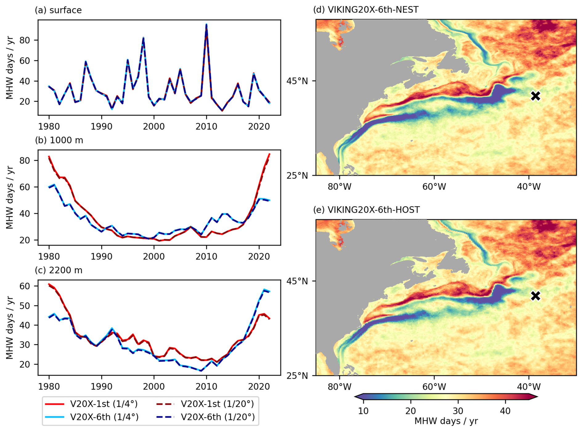
Figure 1 Number of MHW days per year at different depths, derived from the nest ($\mathrm{1}/\mathrm{20}$°) and coarse host ($\mathrm{1}/\mathrm{4}$°) grids (Atlantic only) of the first and sixth cycles in VIKING20X (V20X-1st and -6th). Maps show the mean (1980–2022) number of MHW days per year at the surface derived on the nest and host grids (sixth cycle). The cross indicates the grid point used as an example in Fig. 2.

To detect MHWs along the coasts, the higher-resolution dataset is advantageous due to the more realistic coastline itself. Otherwise, results are still similar along the ocean boundaries (Fig. 1d, e). The same argument holds for the seafloor, which is more realistically represented at higher horizontal resolution. Statistics for larger domains can be calculated on the coarser grid, which significantly decreases the computational costs of detecting MHWs. Accordingly, the following analysis, except for the analysis of bottom MHWs, is carried out on the global host grid of VIKING20X only.

2.4 Heat budget and MHWs in an example region

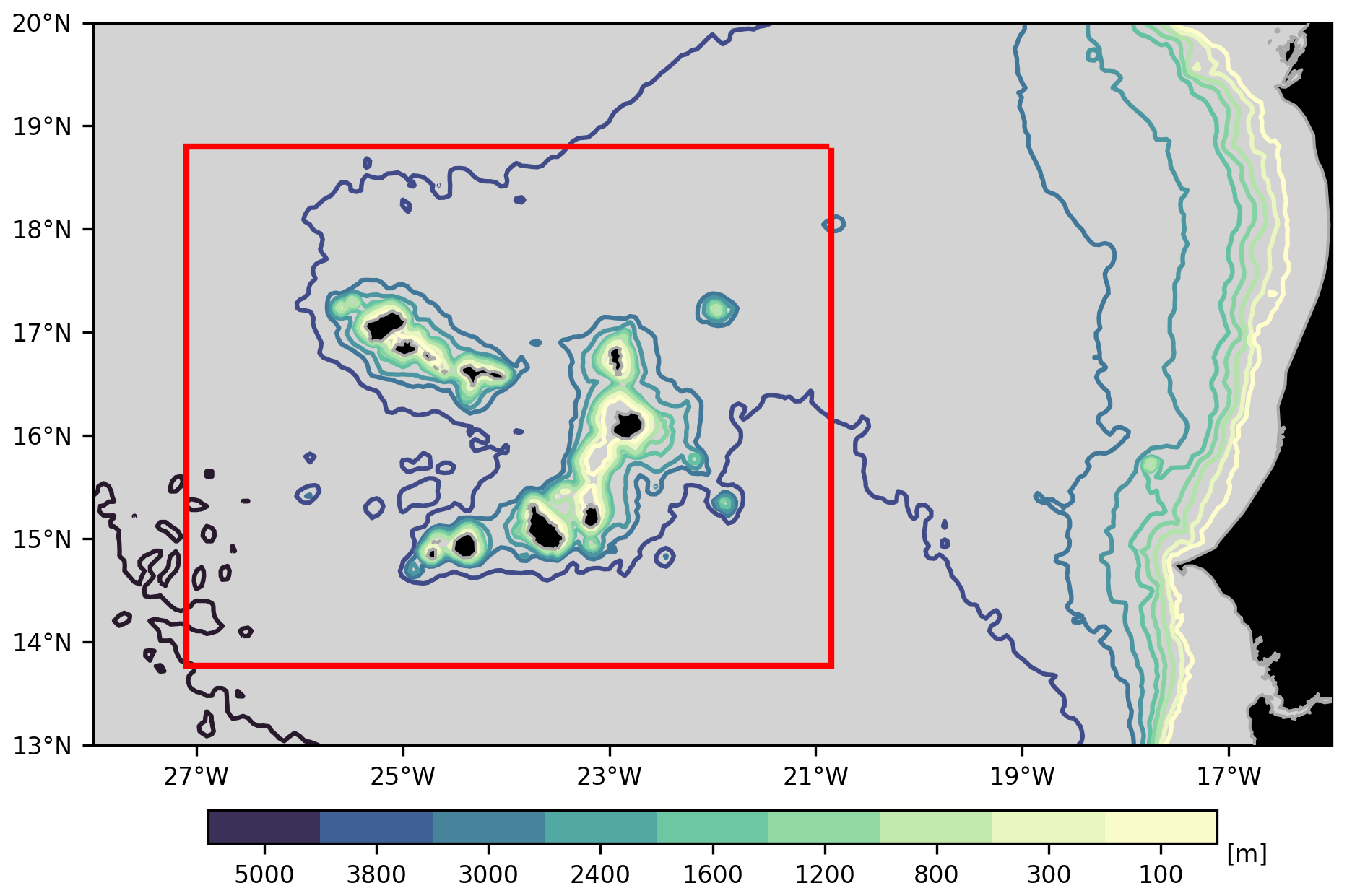
In order to study the vertical coherence and drivers of MHWs in detail, we focus on an example region, here the Cabo Verde archipelago in the eastern subtropical Atlantic (26–22° W, 13.9–18.7° N; see Fig. 8). In order to study the drivers of individual MHW events, well-defined start dates of MHWs in the region are necessary. To obtain such start dates for a larger region and not just a single grid point, individual MHW events are defined at each depth level separately based on the spatially averaged temperature within the region.

To link MHWs to specific drivers, we calculate a heat budget for the same region. The heat content of a given depth level OHC(z) [in J] is calculated from

$$\begin{array}{}\text{(1)}& \mathrm{OHC}\left(z\right)={\mathit{\rho }}_{\mathrm{0}}{c}_p\underset{A}{\int }(T-T_{\mathrm{ref}})\mathrm{\Delta }z\mathrm{d}A.\end{array}$$

Here, A is the area of the Cabo Verde archipelago, and T is the temperature. Following Lee et al. (2004) and Zhang et al. (2018), we use a time-varying, volume-integrated reference temperature for each depth level (T_ref). As a consequence, the horizontal and vertical heat transport reflect external processes rather than internal redistribution of heat. Δz is the grid cell thickness. ρ₀=1026 kg m⁻³ and c_p=3991.87 J kg⁻¹ K⁻¹ are the reference density and specific heat capacity. The values are taken from the NEMO routine that is used to calculate the surface heat flux.

The surface heat flux itself is stored in the NEMO ocean model output and integrated over the same area A.

The ocean heat transport across all sections bounding the area A within a given depth layer OHT(z) [in W] is calculated from

$$\begin{array}{}\text{(2)}& \mathrm{OHT}\left(z\right)={\mathit{\rho }}_{\mathrm{0}}{c}_p\underset{L}{\int }{u}_{\perp }(T-T_{\mathrm{ref}})\mathrm{\Delta }z\mathrm{d}L.\end{array}$$

Here, u_⊥ is the velocity perpendicular to the section. L is a 2D section, and dL is the length of a section segment.

Similarly, the vertical heat transport OHT_w(z) [in W] is calculated from

$$\begin{array}{}\text{(3)}& {\mathrm{OHT}}_w\left(z\right)={\mathit{\rho }}_{\mathrm{0}}{c}_p\underset{A}{\int }w(T-T_{\mathrm{ref}})\mathrm{d}A,\end{array}$$

where w is the vertical velocity.

The residual between ocean heat content change and net horizontal and vertical heat transport (and the surface heat flux if the upper boundary is the ocean's surface) represents all heat budget terms that are missing from the calculations described above. This includes not only horizontal diffusion across the lateral boundaries but also, more importantly, vertical mixing. To link heat content variability to MHWs, we have calculated anomalies relative to the daily climatology using the same procedure as for MHWs. We apply both a fixed_30yr (1980–2009) and detrended baseline. The fixed_30yr baseline was chosen here to represent a fixed baseline approach, as it is generally more common than a 43-year baseline period and differences between the fixed_30yr and fixed_43yr baselines are relatively small (see Sect. 3.1).

The contribution of different heat budget terms to individual MHW events was estimated by calculating the heat gain associated with each term from 2 d before the MHW onset to its peak day. This heat gain was then divided by the total heat content change over the same period. As a result, the sum of all contributions equals 100 %, although individual terms may contribute negatively (i.e., dampen the anomaly) or exceed 100 %. Other lead times prior to the event than 2 d were tested. The results are not sensitive to this choice, as long as the integration does not start within a previous heatwave. To ensure a clear separation of events, we have chosen 2 d (see MHW definition).

3 Results

3.1 Impact of long-term trends on MHW statistics

While the choice of the baseline is important for the interpretation of MHWs at the surface from observations, it is even more important in models. Most models do not just contain “real” trends related to the surface forcing, or changes in circulation, but also trends that arise from an adjustment of the model after initialization (“model drift”; see, for example, Tsujino et al., 2020). This model drift can have a different magnitude and sign at different depth levels (Fig. 2a, b). While, in the top 100 m, the model adjusts quickly and, for the period 1980–2022, trends are similar in the first and sixth cycle, major differences between the cycles occur at greater depth. Around 1000 m, the ocean shows a strong cooling trend in the first cycle, whereas it warms in the sixth cycle. At 2200 m, the ocean warms in the first cycle, whereas it slightly cools in the sixth.

The impact of different baseline definitions on the occurrence of MHWs in the presence and absence of model drift is illustrated in Fig. 2c–h. A location in the deep (2200 m) subtropical North Atlantic is used as an example here (see black cross in Fig. 1d, e). The temperature in the first cycle shows pronounced multi-decadal variability, with high temperatures during the first and last 10 years of the time series and lower temperatures in between. In the presence of strong model drift (first cycle), multi-decadal variability is captured by the MHW statistics only when a detrended baseline is used. With the two fixed baselines, a linear trend in the temperature causes MHWs to occur predominantly in the later period. This is different in the sixth cycle, where, in the absence of model drift, the different baselines yield more similar results. Also, for the detrended baseline, the results are more similar between the two cycles.

On the one hand, this suggests that the MHWs derived at this particular location in the first cycle are dominated by unrealistic drift, except when a detrended baseline is used. On the other hand, it suggests that the linear temperature trend over the last 40 years was of minor importance in the deep (2200 m) subtropical North Atlantic when model drift is absent (sixth cycle). Instead, changes in the occurrence and characteristics of MHWs were dominated by (multi-)decadal variability, independent of the baseline used for detection.

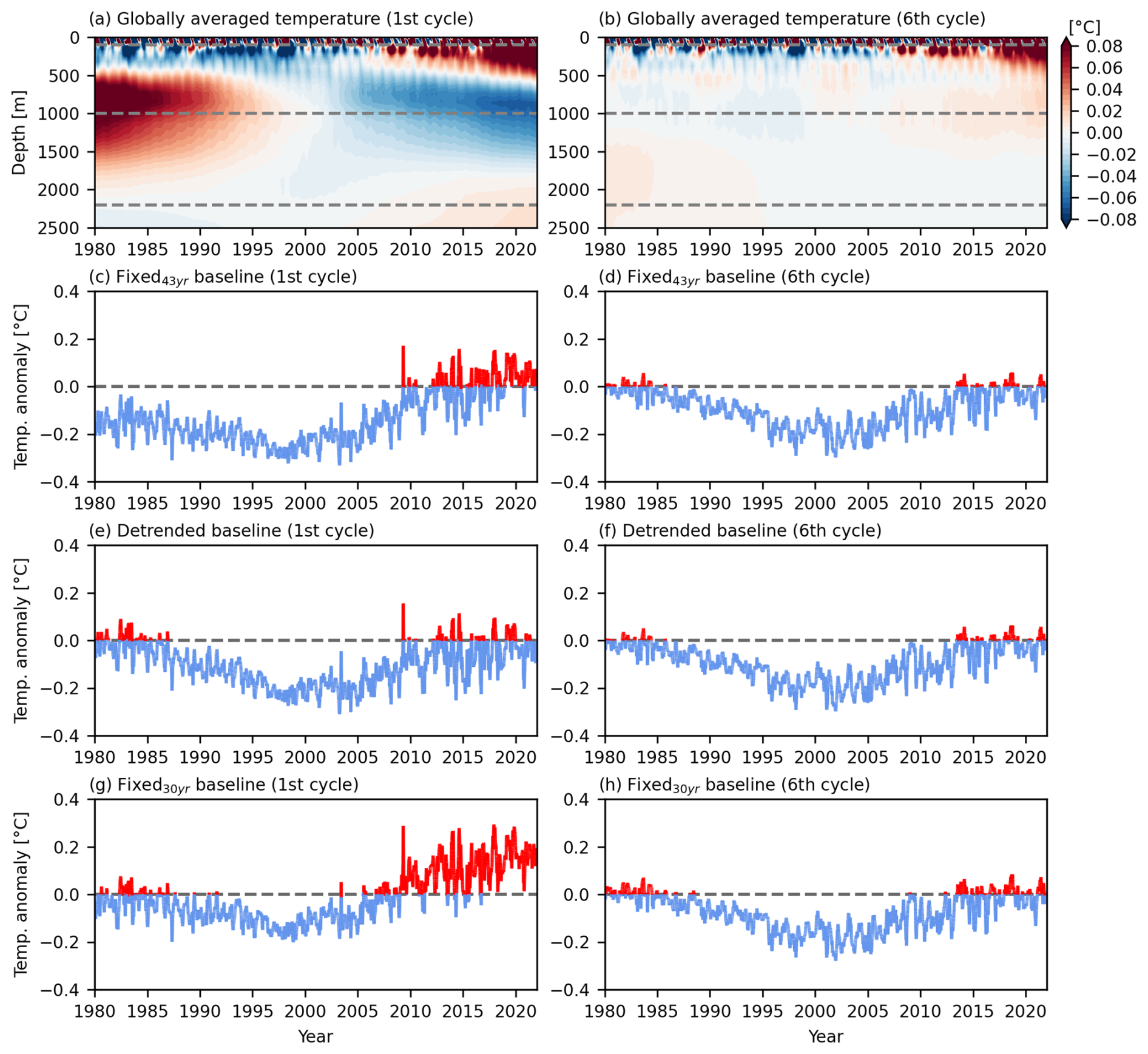
Figure 2 Globally averaged temperature anomaly relative to the 1980–2022 mean, illustrating model drift (a, b). Temperature relative to the MHW threshold estimated with different baselines at 41.8° N, 38.6° W (see cross in Fig. 1d, e) at 2200 m depth (c–h).

The impact of the model's temperature drift is directly reflected in the basin-wide MHW statistics as well. At the surface and at 100 m depth, MHW statistics are robust across the cycles (Fig. 3a, b, upper two rows), suggesting that the trend is mostly caused by the common surface forcing. In contrast, a strong drift in the temperature of the first cycle leads to major differences at depth if the fixed baselines are applied (Fig. 3a, b, lower two rows). At 1000 m depth, the number of MHW days is small before and increases after 2000 in the sixth cycle. Conversely, it shows a sharp decline in the 1980s and then stays near zero in the first cycle. At 2200 m, the ocean reaches a near-permanent MHW state toward the end of the time series (365 MHW days per year) in the first cycle. The strong increase in MHW days is more pronounced with the fixed_30yr compared to the fixed_43yr baseline. This is because the threshold at 2200 m is lower when the last 10 years are not included, as the mid-depth ocean was anomalously warm in the 2010s in most regions (see Fig. 2 as an example). In contrast, the sixth cycle shows a decrease in MHW days from around 100 to almost no MHW days per year after the 1990s.

Relative to a fixed baseline, the evolution of the MHW statistics is dominated by the impact of model drift in the first cycle. Using a detrended baseline not only removes most of the model drift but also removes any forcing-related trends. This is particularly visible at the surface and at 100 m depth (Fig. 3a, b, upper two rows). As it is not possible to know from the experiments themselves which part of the trend is related to the forcing and which part to model drift, there is no method to recover the fixed baseline statistics of the sixth cycle from the first cycle. As a consequence, the first cycle cannot be used to make any statements about the long-term evolution of MHWs at depth relative to a fixed baseline.

Applying the detrended baseline yields more similar, but not identical, results in the presence (first cycle) and absence (sixth cycle) of model drift (red lines in Fig. 3a, b, lower two rows). While the correlation between the time series of the first and sixth cycle is higher than 0.9 at the surface and at 100 m for all baselines, there is a weak anticorrelation (about −0.3) at 1000 and 2200 m for the fixed baselines. The detrended baseline time series are still highly correlated between the first and sixth cycles at 1000 m (0.91) and at 2200 m (0.85). Detrending also leads to a similar evolution of the temperature itself in both cycles (e.g., Fig. 2e, f). This is also true for the global mean temperature at all depth levels (not shown). Assuming that model drift adds linearly to forced temperature trends is therefore reasonable, but non-linear adjustments are not completely absent. A non-linear shifting baseline was tested (not shown) as well, but it yielded no advantage over the detrended baseline. In agreement with Chiswell (2022), differences in the derived MHW statistics are small. Further, the non-linear shifting baseline has disadvantages due to the finite length of the time series. A moving average leads to a loss of data at the beginning and end of the time series, or the averaging window has to be modified at the beginning and towards the end, which can introduce spurious signals. Therefore, the non-linear shifting baseline is not discussed further in this paper.

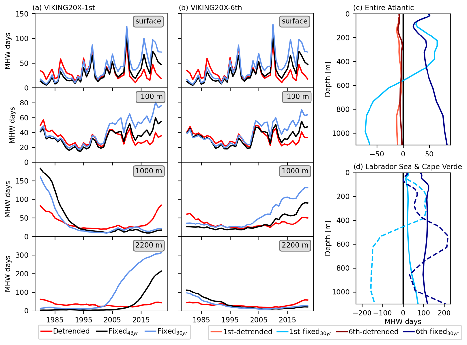
Figure 3 Number of MHW days per year averaged over the Atlantic in the first, strongly drifting (a) and sixth, equilibrated (b) cycle at selected depths and for different baselines. Depth profiles of the difference in the number of MHW days between the last 10 years (2013–2022) and the first 10 years (1980–1989) for the entire Atlantic (c) and for the Cabo Verde archipelago (d; dashed) and Labrador Sea (d; solid). For the entire Atlantic, the detrended and fixed_30yr baselines are shown, whereas in (d), only results from the fixed_30yr baseline are shown.

Vertical profiles of the differences between the last and first 10 years of the time series further reveal that only in the top 100 m are the statistics comparable between the first and sixth cycle when the fixed_30yr baseline is used (Fig. 3c). Below 100 m depth, the number of MHW days shows a stronger increase from the beginning to the end of the time series in the first cycle. Below 600 m depth, changes are of the opposite sign in the first and sixth cycle. Thus, model drift dominates the long-term changes in MHW statistics of the first cycle below approximately 100 m depth. When using a detrended baseline, changes in the mean temperature between the decades are mostly removed, and the resulting changes in MHW days are almost zero. This indicates that changes in the shape of the temperature distribution (standard deviation, skewness) that could lead to differences between the decades with a detrended baseline played a minor role.

There are regional differences, however (Fig. 3d). For example, in the Labrador Sea (solid), the results differ already at the surface. In the eastern subtropical Atlantic (Cabo Verde archipelago; dashed), the changes are similar within the top 50 m. This highlights that the impact of model drift is not the same everywhere. Note that the surface flux is (almost) the same in the first and sixth cycle and thus cannot explain differences between the cycles. In regions where ocean advection and stratification play an important role near the surface, model drift is likely to affect the occurrence of MHWs at depths even shallower than 100 m. This is the case for the Labrador Sea, where advective processes strongly influence the mixed layer dynamics (e.g., Gelderloos et al., 2011). For the Cabo Verde archipelago, the variability in the mixed layer, which, in the annual mean, extends to approximately 70 m depth, is strongly influenced by the surface heat flux, as will be shown later (Sect. 3.4).

In the following, we focus on the characteristics of MHWs detected by applying the fixed_30yr baseline in the sixth cycle. As argued above, the first cycle can only be used to study MHWs defined based on the detrended baseline, but we are explicitly interested in studying the impact of long-term changes in the surface forcing and ocean circulation on MHWs. Because including the trend requires a very long model spin-up that is rare at $\mathrm{1}/\mathrm{20}$° resolution, this provides unique and novel insights into the characteristics of MHWs and the impact of long-term temperature changes. Even though temperature trends in the deep ocean are highly uncertain due to the lack of long-term observations, the well spun-up sixth cycle is regarded as the best estimate available.

3.2 Horizontal and vertical changes in MHW characteristics

3.2.1 Characteristics of MHWs at the surface

Compared to the observation-based NOAA OISST dataset (Huang et al., 2021), VIKING20X overestimates the duration but underestimates the maximum intensity of MHWs at the surface throughout most of the Atlantic (Fig. 4; fixed_30yr baseline). This is a well-documented feature of many models compared to satellite-based datasets (Qiu et al., 2021; Pilo et al., 2019). A notable exception is the northern flank of the Gulf Stream (GS), where VIKING20X simulates higher maximum intensities. The temporal variability of the basin-averaged statistics is in very good agreement, however (Fig. 4g–i). The correlation exceeds 0.66 for all time series. While the magnitude of the variability is similar for the frequency and maximum intensity, it is higher for the MHW duration in the model. The duration and frequency show a positive linear trend, which is slightly stronger in the NOAA OISST dataset. The maximum intensity does not show a clear trend in either of the two datasets.

The horizontal patterns of the time mean frequency and maximum intensity match the observation-based product as well (note the difference in the color bar that represents the mentioned mean bias). A high frequency of MHWs is seen along the Equator, in the western North Atlantic subtropical gyre and in a zonal band around 30° S (Fig. 4b, e). Only few MHWs per year are detected within 20° around the Equator and in the eastern subpolar gyre in both the model and observations. The GS, boundary currents of the subpolar gyre and the upwelling regions along the eastern boundary stand out with high maximum intensities (Fig. 4c, f). Differences between the datasets are more pronounced for the duration of MHWs (Fig. 4a, d). In particular, between the Equator and 20° N, VIKING20X shows very long MHWs, but OISST shows very short MHWs. In most other regions, the model and satellite data agree on whether MHWs are comparably long or short (e.g., long MHWs north of the GS separation and short around the UK), but VIKING20X generally overestimates the duration. Differences in duration are largest in regions that show high cloud cover, especially in the Intertropical Convergence Zone (ITCZ), limiting the availability of satellite-based SST. This may contribute to the larger difference in these regions compared to other parts of the Atlantic. Nevertheless, it cannot be concluded that the model is more realistic, and model biases could play an important role too. For example, the vertical resolution of the model can be important in regions that develop very shallow mixed layers during surface-forced MHWs. The heat gained through the surface is then mixed over a smaller volume, which may not be adequately simulated by a model with too coarse vertical resolution.

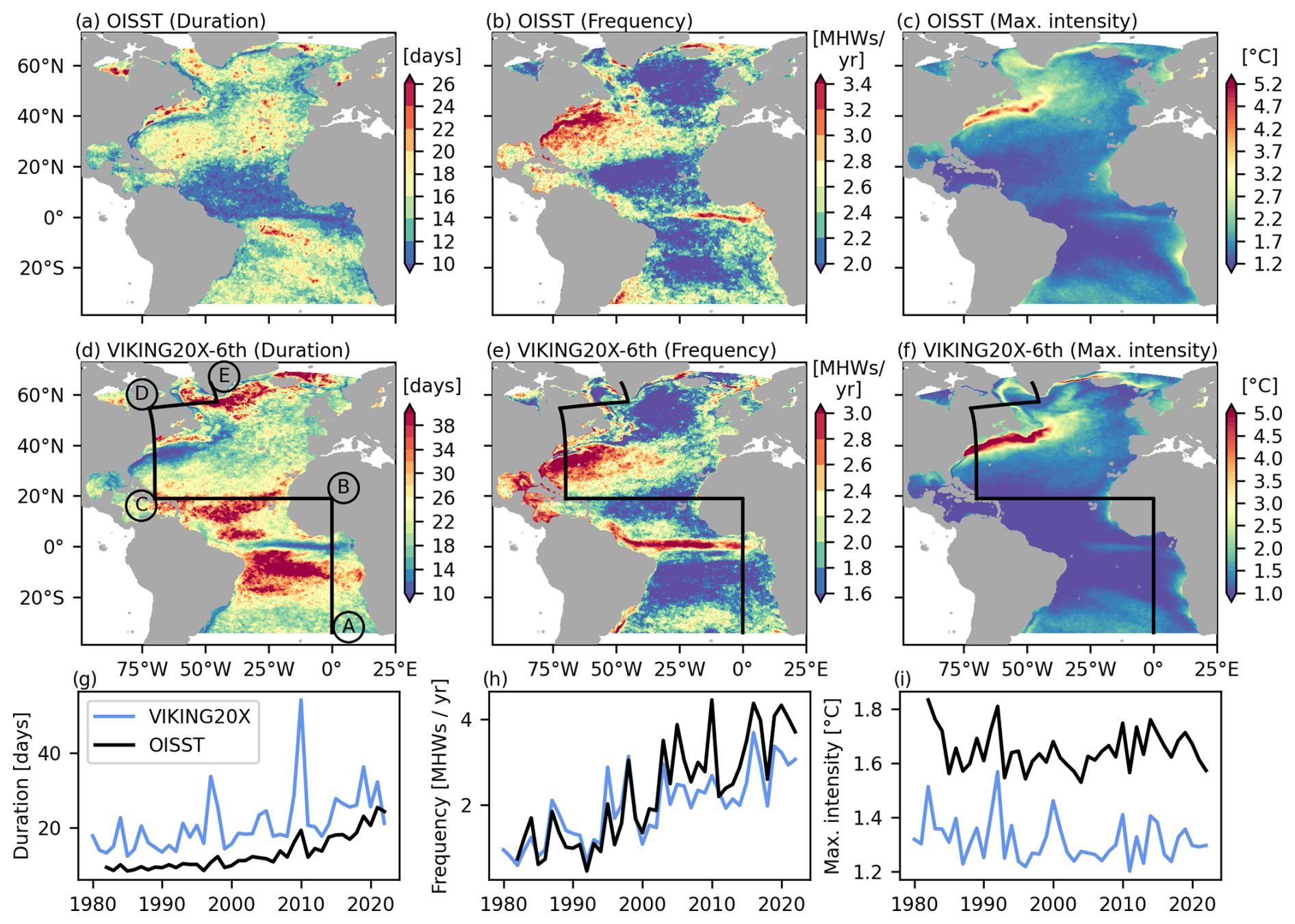
Figure 4 Mean (1982–2022) duration, frequency and maximum intensity of MHWs at the surface in the NOAA OISST dataset (a–c) and the sixth cycle of VIKING20X (d–f). The black line in (d)–(f) indicates the section shown in Fig. 5 (letters mark the section vertices). Time series show the annual mean MHW characteristics averaged over the Atlantic from both datasets (g–i).

3.2.2 Characteristics of MHWs at depth

A section through the Atlantic (see black lines in Fig. 4d–f) shows that the characteristics of MHWs considerably vary in the horizontal as well as in the vertical plane (Fig. 5). The section was chosen to compare the vertical structure of MHWs in dynamically very different regions, starting in the South Atlantic, crossing the Equator, the Mid-Atlantic Ridge, the western boundary current system and finally the deep convection region in the subpolar gyre. MHWs in the abyssal ocean last long but occur rarely. Duration and frequency are directly related, as MHWs that last a year can, by definition, only occur once a year. The only exception is the eastern subtropical gyre, between Puerto Rico and Canada, where relatively short MHWs occur at abyssal depth. However, the abyssal ocean (deeper than approximately 4500 m) may not have fully adjusted even after more than 300 model years. Therefore, the abyssal ocean should be interpreted with caution. Another maximum in MHW duration along the section occurs between 1000 and 2000 m. In the subpolar gyre, between Canada and Greenland, very long MHWs occur between 300 and 3000 m depth (Fig. 5a).

There is a general tendency for MHWs to be longer in regions where the frequency is lower (Fig. 5a, b), but compared to the duration, the frequency shows stronger differences along the section at the same depth level. The frequency is generally higher along the boundaries. For example, in the eastern upwelling regions (around Africa) and within the western boundary currents (around Puerto Rico), the highest frequency is not reached at the surface but between 500 and 1000 m depth. In the subpolar gyre, the maximum frequency is reached at even great depths.

The maximum intensity peaks at the surface along the entire section (Fig. 5c). Outside the tropics, a secondary maximum occurs at depths around 500 m. Below 1000 m, the maximum intensity does not exceed 0.1 °C in most regions. Within energetic currents, for example, the Deep Western Boundary Current (DWBC) close to Puerto Rico and the GS, the intensity is higher and can reach up to 0.2 °C even beyond 3000 m depth (Fig. 5c). Also, around the Mid-Atlantic Ridge (MAR), the maximum intensity is elevated. In the deep convection region in the western subpolar gyre (between Greenland and Canada), the maximum intensity is higher than 0.1 °C down to 2500 m depth.

Overall, the sections show that MHWs are more frequent and intense in regions of strong current variability and/or strong gradients in mean temperature. The presence of deep currents leads to pronounced sub-surface maxima in frequency and intensity, with a tendency for comparably short MHWs. Variability linked to deep convection in the central Labrador Sea (between Greenland and Canada) causes intense MHWs below 1000 m depth as well, but they last longer and occur less frequently than MHWs along the deep boundaries.

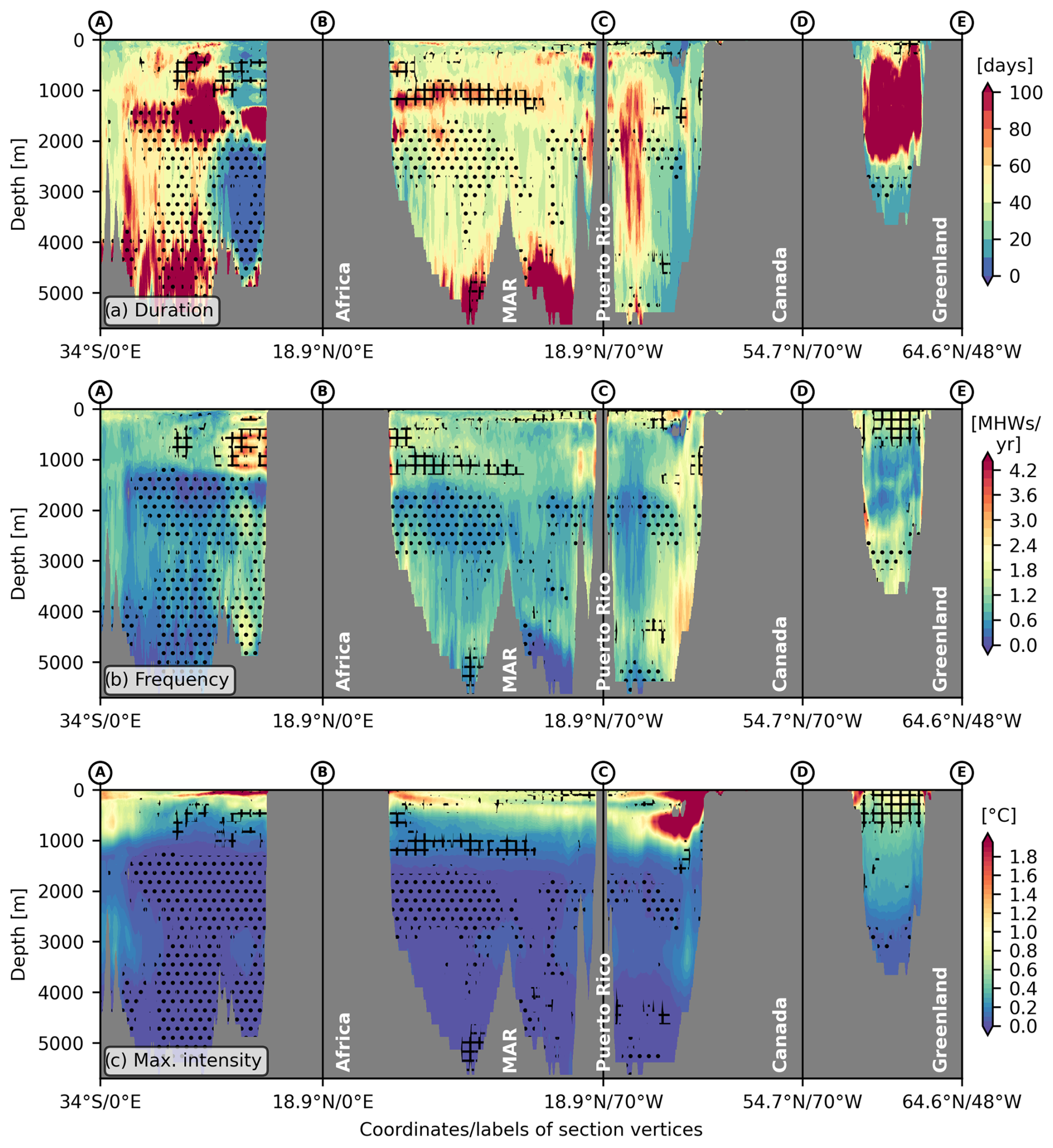
Figure 5 Mean (1980–2022) duration, frequency and maximum intensity of MHWs along a section through the Atlantic Ocean (see Fig. 4) based on the sixth cycle of VIKING20X and applying the fixed_30yr baseline (shading). The sign of the linear trend (1980–2022) at the same grid points is indicated by crosses (positive trend) and dots (negative trend). They are drawn only where the trend is significantly different from zero based on a 5 % significance level.

Many studies and the VIKING20X model agree on an increase in MHW frequency, duration and intensity at the surface (Xu et al., 2022; Oliver et al., 2018; Chiswell, 2022). The magnitude and sign of linear trends are not uniform across the ocean, however. The duration of MHWs increased in the tropical Atlantic (around point B) between 500 and 1500 m depth (crosses in Fig. 5a). The South Atlantic (between points A and B) shows a significant decrease in duration (dots in Fig. 5a) below 2000 m, while the tropical and subtropical North Atlantic (B to D) show such a decrease only between 2000 and 3500 m. Regions of positive trends in duration are also subject to a positive trend in frequency and maximum intensity (Fig. 5b, c). This may seem to contradict the previous description, as MHWs in regions of higher mean frequency tend to be shorter. At the same time, it is expected, as a warming leads to the threshold being exceeded more often and for longer. A distinct pattern can be seen in the subpolar gyre (D to E). Here, positive trends in all characteristics occur at the surface and negative trends around 3000 m (Fig. 5a–c), which can be explained by a reduction in deep convection. A near-surface warming increases the MHW intensity, duration and frequency but also reduces the mixed layer depth. The shallower winter mixed layers then prevent mixing between the deep waters (that are no longer reached by the mixed layer) and the upper ocean waters. Below 3000 m, the boundary currents are colder than the interior Labrador Sea, likely causing a cooling in the absence of exchange with the surface.

3.2.3 Bottom MHWs

As the seafloor provides a unique habitat for various marine species, the detection of MHWs along the seafloor rather than at a fixed depth is of major interest for the biological community. Bottom MHWs are defined here as MHWs that occur in the last ocean-filled model grid cell above the bottom.

Figure 6 Mean (1980–2022) duration, frequency and maximum intensity of MHWs at the bottom (fixed_30yr baseline; VIKING20X-6th nest grid; a–c). The linear trend is shown in the lower panels (d–f). Significant trends (5 % significance level) are indicated by dots. A bottom depth of 5000 m is indicated by the white contour.

The deep ocean basins with depths exceeding 5000 m are characterized by very long but infrequent MHWs (Fig. 6a, b). The duration of MHWs exceeds a year, and therefore the low frequency is a direct consequence, as already mentioned above. Additional analysis performed on bottom MHWs detected with a detrended baseline (not shown) suggests that the bottom water masses are experiencing a long-term warming trend. The source of the long-term warming trend cannot be known, but the bottom water masses are probably still subject to model drift, even after more than 300 years of model spin-up, due to the long adjustment timescale of the abyssal ocean. This leads to a near-permanent heatwave state in the beginning or at the end of the time series. Although their maximum intensity remains below 0.1 °C (Fig. 6c), the temperature tolerance of most deep sea species is highly uncertain, and the possible impact of such low-intensity but long-lasting MHWs has yet to be determined.

It is interesting to note that, even though very deep, the North American Basin is characterized by rather short MHWs (Fig. 6a, b). This suggests that the high variability associated with the GS impacts temperature extremes down to the seafloor. In general, bottom MHWs are shorter near the continental slopes compared to the abyssal plains and Mid-Atlantic Ridge. This is not just related to different depths, as the bottom along the lower continental slope is deeper than parts of the Mid-Atlantic Ridge. The frequency of bottom MHWs is highest along the continental slope (Fig. 6a, b). Notably, it is higher along the slope than it is on the shelf, which is related to the sub-surface maxima along the slope seen in Fig. 5. High frequencies are seen along the western boundary following the DWBC pathway, along the pathways of the overflow water in the subpolar gyre and along the eastern boundary. The maximum intensity strongly follows the bathymetry, with the highest intensities reached on the shelf. Further, the intensity is higher along seamount chains and the Mid-Atlantic Ridge where the seafloor is elevated (Fig. 6c).

Bottom MHWs on the shelves show an increase in frequency, duration and maximum intensity over time (Fig. 6d–f). The linear trend in these MHW characteristics is not significant everywhere on the shelf and along the upper continental slope, due to strong interannual variability. Significant positive trends in frequency, duration and maximum intensity can be seen in the eastern subtropical North Atlantic and the western tropical Atlantic. Significant negative trends occur in the subpolar gyre, the Caribbean Sea, and the entire eastern tropical and subtropical South Atlantic. Again, trends in the deep ocean are associated with higher uncertainties, due to the lack of long-term observations. In particular, the abyssal plains may be still subject to model drift.

3.3 The impact of mesoscale dynamics on the characteristics of MHWs

The previous sections suggest that the presence of strong and highly variable currents has an important impact on the characteristics of MHWs. To test how the representation of mesoscale dynamics impacts the characteristics of MHWs, we compare the sixth cycle in VIKING20X to the sixth cycle in the un-nested ORCA025 configuration. The sixth cycle is chosen here because we aim to compare MHWs in an adjusted ocean state. The temperature drift (and thus MHW statistics) is different in ORCA025 and VIKING20X throughout the first cycles, such that the results of earlier cycles are not directly comparable. The higher horizontal resolution leads to the presence of individual mesoscale features in VIKING20X, of which only a small part is simulated in ORCA025 outside the subtropics (Biastoch et al., 2021). It also leads to changes in the mean current structure and position, as well as differences in temperature trends and in horizontal and vertical temperature gradients (Fig. A1 in the Appendix). All these aspects may have an impact on the characteristics of MHWs.

The VIKING20X dataset contains the imprint of mesoscale dynamics throughout the Atlantic as discussed above, although, for both configurations, MHWs are detected on a $\mathrm{1}/\mathrm{4}$° grid. Results are shown only for the fixed_30yr baseline, but the conclusions do not depend on the baseline.

At 1000 m depth, VIKING20X shows a high frequency of MHWs along the western and eastern boundaries as well as along the Equator (Fig. 7a). Compared to ORCA025, the frequency in VIKING20X is higher almost everywhere, but in particular along the western boundary and eastern boundary outside the tropics (Fig. 7c, e). At the western boundary, this goes along with a stronger, more narrow and more variable western boundary current in VIKING20X. This is apparent by the difference in mean and eddy kinetic energy (MKE/EKE) in the two configurations. Also, vertical velocity fluctuations (vertical velocity EKE) are stronger along the western boundary in VIKING20X (Fig. A1a–c). Along the eastern boundary, differences in MKE are relatively small, but EKE is still higher at least north of the Equator. Also, the horizontal and vertical temperature gradients are larger in VIKING20X (Fig. A1d, e). When averaged over the entire Atlantic, the temporal evolution of the MHW frequency is similar (correlation of 0.94), but the mean frequency is clearly higher in VIKING20X (Fig. 7e). Although it is not possible to prove that the higher frequency in VIKING20X is more realistic, it is expected that the more realistic representation of currents and their variability leads to more realistic MHW characteristics in VIKING20X.

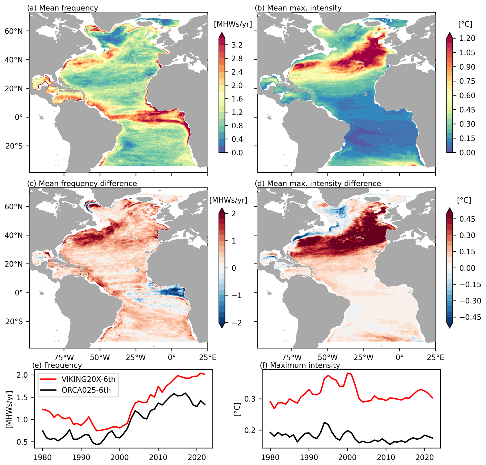
Figure 7 Mean (1980–2022) MHW frequency and maximum intensity at 1000 m depth in the sixth VIKING20X cycle (a, b). Difference between VIKING20X (sixth cycle) and ORCA025 (sixth cycle) (c, d). Time series show the average over the Atlantic from both experiments (e, f). In all panels, MHWs are defined using the fixed_30yr baseline.

The maximum intensity shows a strong maximum in the region of the GS separation at 34° N (Fig. 7b). Also, in the eastern Atlantic between 40 and 60° N, the mean maximum intensity exceeds 1.2 °C. In this area, the transition between the warm Mediterranean Sea Outflow Water and colder North Atlantic Deep Water or Subarctic Intermediate Water is located at approximately 1000 m depth (Kaboth-Bahr et al., 2021; Liu and Tanhua, 2021). The transition between these water masses of different temperature is related to a strong vertical temperature gradient (see Liu and Tanhua, 2021). Therefore, vertical displacements of isotherms, for example, through internal waves or other vertical velocity anomalies, can cause strong temperature anomalies in these regions. High values of maximum intensity are further seen west of Greenland, where flow instabilities lead to the shedding of West Greenland Current eddies and Irminger Rings, which are typical expressions of the mesoscale resolution in this region (Biastoch et al., 2021; Rieck et al., 2019). Along the western boundary, south of the DWBC/GS crossover, the maximum intensity is higher than in the interior as well. Compared to ORCA025, VIKING20X simulates more intense MHWs (Fig. 7d, f). The difference is strongest in the regions where the mean maximum intensity is highest. West of Greenland, this is directly linked to the presence of mesoscale eddies in VIKING20X as described above. The presence of Irminger Rings that transport warm water from the Irminger Current into the cold central Labrador Sea in VIKING20X is likely related to the occurrence of strong MHWs. The negative difference north and positive difference south of the GS pathway suggest a more southern position of the GS in VIKING20X. This is supported by the MKE and horizontal temperature gradient differences (Fig. A1a). Higher intensities are seen along most of the western boundary, related to a stronger horizontal temperature gradient and higher EKE (Fig. A1c, e). In the eastern North Atlantic, the vertical temperature gradient is stronger in VIKING20X (Fig. A1d), which can explain the higher maximum intensities.

Overall, the more realistic representation of boundary currents and coastal upwelling and the ability to resolve sharper temperature gradients lead to a higher frequency (and shorter duration) and higher maximum intensity of MHWs throughout most of the Atlantic, but in particular along the western boundary. This was shown only for the depth of 1000 m, but similar arguments apply at least to the depth range from 300 to 3000 m (not shown).

3.4 Vertical structure and drivers of MHWs in an example region

In order to better understand the vertical structure and coherence of MHW events, we now focus on the Cabo Verde archipelago in more detail. The Cabo Verde archipelago is located in the eastern tropical Atlantic in between the westward flowing North Equatorial Current and eastward North Equatorial Counter Current. It is part of the Canary Current upwelling system and thus characterized by large-scale upwelling (Arístegui et al., 2009; Cropper et al., 2014).

This region is selected here as an example due to its high species richness, including the presence of vulnerable marine ecosystem (VME) indicator species (Vinha et al., 2024; Hoving et al., 2020; Stenvers et al., 2021) and large bottom depth gradients (see Fig. 8) such that benthic ecosystems span a large depth range in a horizontally confined region. As a result, one might expect MHWs to have important impacts beyond the surface, and thus a detailed understanding of their characteristics throughout the water column is highly relevant. Additionally, the eastern subtropical Atlantic is interesting in the context of this study, as it shows significant trends in the MHW characteristics that change sign at approximately 1500 m depth (Fig. 5).

Figure 8 Depth of the seafloor in the eastern tropical Atlantic. The Cabo Verde archipelago region (red) is used for the spatial averages in Figs. 9, 10 and 11.

3.4.1 Variability of MHW characteristics

The characteristics of MHWs at the surface and below 50 m depth do not vary coherently (Fig. 9a–c). For example, a period of short MHWs in the 2010s near the surface coincides with a period of anomalously long MHWs between 100 and 1300 m. Already, at 100 m depth, the explained variance (squared correlation coefficient R²) by their respective surface values has dropped to values below 25 % for all MHW metrics (Fig. 9d–f). This means that variability of the surface metrics, which are strongly linked to variability of the surface heat flux as will be shown later, accounts for only a small fraction of the variance in the MHW characteristics at depth. This is consistent with the impact of surface-forced trends being limited to about 50 m depth in the Cabo Verde archipelago, as discussed above (Fig. 3). Different long-term trends could decouple surface MHWs from deeper MHWs regardless whether the drivers of individual heatwaves act coherently across a larger part of the water column. However, removing the linear trend of the MHW characteristics itself or detecting MHWs with a detrended baseline leads to the same results (Fig. 9d–f). This suggests that the different drivers of variability on shorter timescales rather than different long-term trends are the main reason for the low correlation between the MHW metrics at the surface and at greater depths.

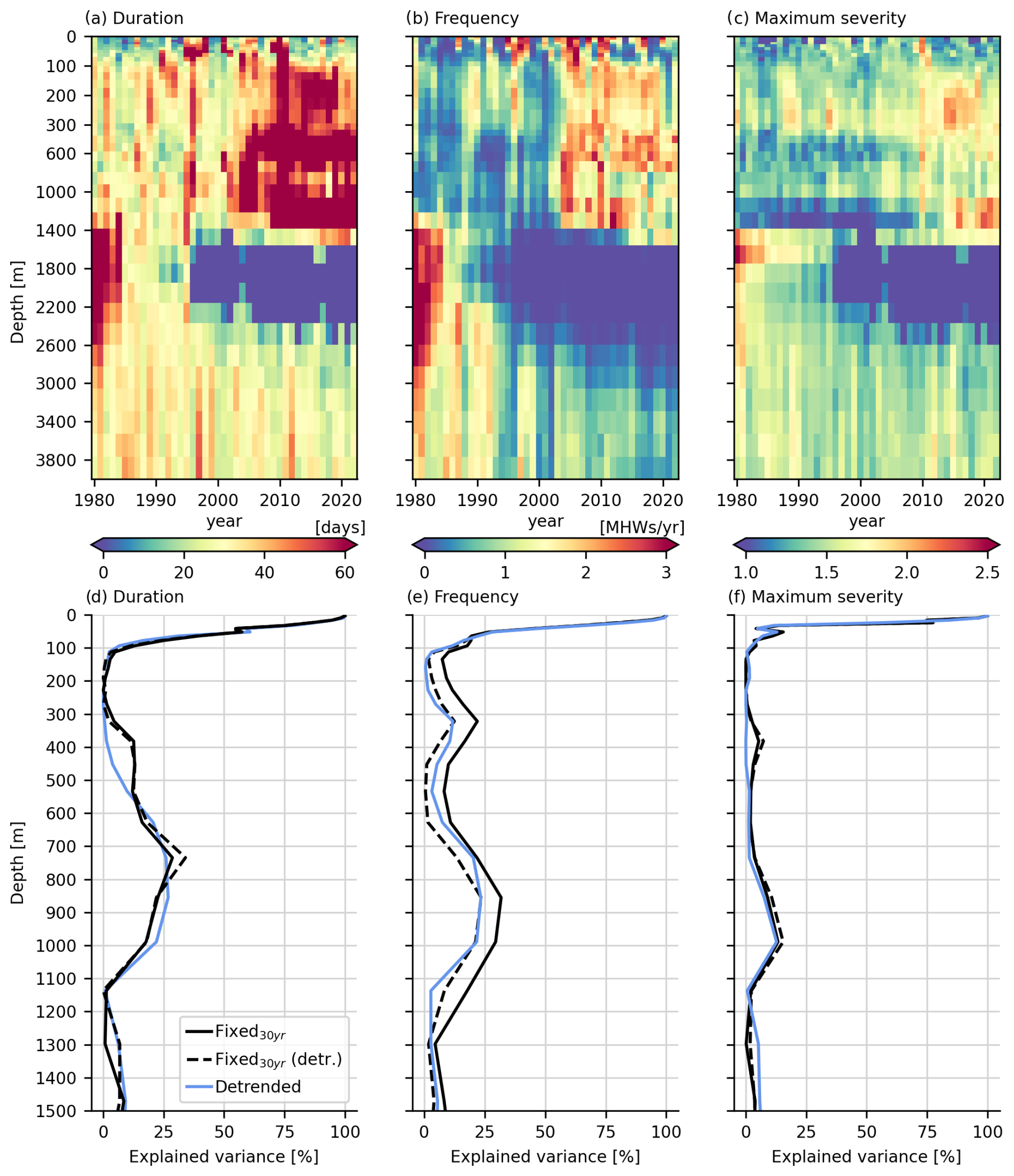
Figure 9 Annual mean MHW duration, frequency and maximum severity in the Cabo Verde archipelago (fixed_30yr baseline; VIKING20X-6th; a–c). Explained variance of the MHW duration, frequency and maximum severity at different depths by their annual mean values at the surface (d–f). The explained variance was calculated for the fixed_30yr baseline (black, solid) and for the detrended baseline (blue). Additionally, the dashed lines represent the explained variance based on the same fixed_30yr baseline detection, with the trend in the MHW characteristics removed.

Annual mean duration, frequency and maximum severity are subject to pronounced interannual variability near the surface. In deeper layers, low-frequency variability is more dominant (Fig. 9a–c), which leads to a lower explained variance. In the late 2000s, an increase in MHW duration, frequency and maximum severity seems to propagate from the surface towards sub-surface layers above 300 m. Thus, there might be a connection between surface MHWs and MHWs in the upper 300 m even though they do not have the same characteristics nor appear at the same time. Instead of the maximum intensity, we show the maximum severity here, which is defined as the ratio of the maximum intensity and the difference between the climatological mean and 90th percentile (Sen Gupta et al., 2020). The severity index compares the anomaly to the magnitude of local variability, which is much lower in the deep ocean. It is interesting to note that the maximum intensity is much stronger near the surface (see, for example, Fig. 5c), but the maximum severity shows similar values at all depth levels (Fig. 9c). This means that, relative to the typical range of temperature variability, the anomaly associated with MHWs is similarly strong at all depths.

Between 300 and 1300 m, MHW characteristics vary coherently, with low values for all variables before 2000 and higher values afterwards (Fig. 9a–c). For this depth range, no connection to the surface can be identified, even when possible time delays are considered. Between 1300 and 3000 m, long and intense MHWs occur frequently at the beginning of the time series, and nearly no MHWs occur after 1995. Between 3000 and 4000 m, there is a small (compared to other depth layers) decreasing trend in frequency and duration, but variability on interannual timescales dominates the time series. It is important to remember that the MHW definition was applied at individual grid points and depth levels and does not include any spatial information (see methods). Still, MHW characteristics exhibit a similar temporal evolution over broader depth ranges. This is mostly not related to the surface forcing but rather to other processes that act coherently over certain depth ranges. These processes are investigated in more detail in the following.

3.4.2 Vertical coherence of individual MHWs

In order to understand which drivers control the variations of MHW characteristics at different depths, we now consider individual MHW events in the Cabo Verde archipelago. In general, the annual mean characteristics described before (Fig. 9a, b) are also reflected by the individual events (Fig. 10a, b). The mixed layer is characterized by relatively short, intermittent events. By comparing the results from MHWs detected using the fixed_30yr and detrended baselines (Fig. 10a, b), it is evident that the linear trend within the mixed layer had a minor impact on the occurrence of MHWs in the Cabo Verde archipelago. In contrast to deeper depth levels, the timing of MHW events is similar between the two baselines near the surface. The mixed layer (here, the maximum mixed layer within the region) shows a seasonal cycle from 20 m in summer to 100 m in winter. In several years (e.g., 1995, 1998, 2005, 2010), MHWs occur in the mixed layer when it is deep during winter and remain below the mixed layer as it shoals in summer (Fig. 10a, b). While MHWs are then often terminated in the mixed layer, presumably due to surface fluxes, they persist below. This leads to different characteristics of MHWs in the top 50 m and the depth layer between 50 and 100 m, but MHWs may still be initially forced by a heat gain through the surface.

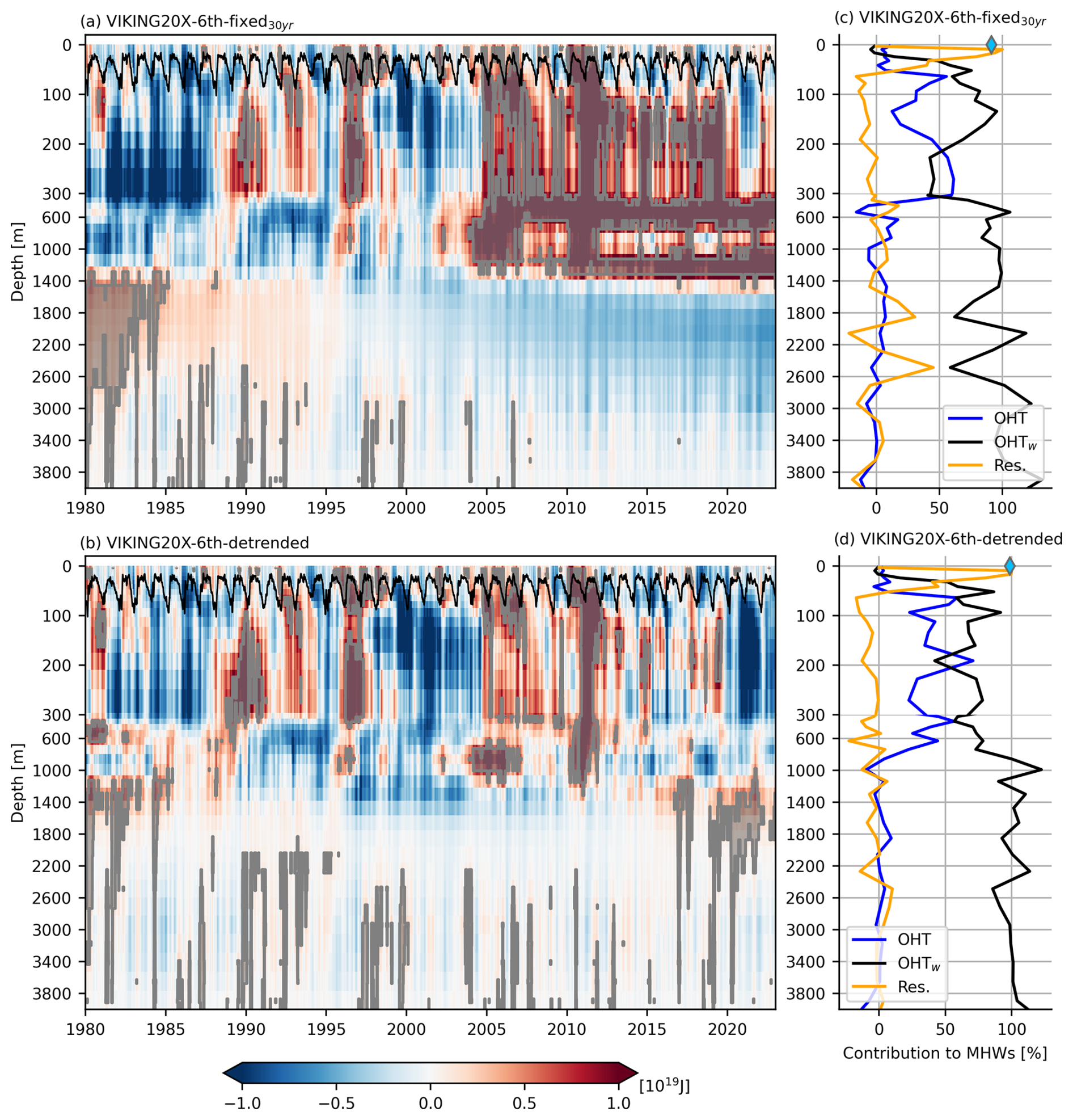
Figure 10 Cabo Verde archipelago ocean heat content anomaly (relative to the 1980–2009 daily climatology; a) and detrended ocean heat content anomaly from the daily climatology (b). The black line indicates the maximum mixed layer depth within the region. MHW events detected in the sixth cycle of VIKING20X with the fixed_30yr (a) and detrended (b) baselines are shaded in gray. Vertical profiles of the contribution of different heat budget terms to individual MHW events detected with the fixed_30yr (c) and detrended (d) baselines. The contributions were averaged over all MHWs that occur at a particular depth. OHT – horizontal ocean heat transport, OHT_w – vertical ocean heat transport, Res. – residual flux. Diamonds indicate the surface heat flux contribution in the uppermost model level.

Below 100 m depth, some MHWs are connected to surface MHWs (e.g., 1995, 2005, 2010), in particular when using the fixed_30yr baseline (Fig. 10a, b). In other years, MHWs occur without any apparent link to the surface (e.g., 1990 for both baselines; 2014 and 2020 with the detrended baseline). Therefore, the depth range between 100 and 300 m is governed not only by the surface exchange of heat but also by other processes. The heat content and occurrence of MHWs show a stronger positive trend in this depth range compared to the surface (Fig. 10a). MHWs detected based on the detrended baseline also occur more often between 2004 and 2020, but they are generally shorter (Fig. 10b). This indicates that both decadal variability and a long-term trend cause the strong increase in MHW coverage seen with the fixed_30yr baseline.

Beyond 300 m depth, coherent MHWs occur over layers of a few hundred to 1000 m thickness (Fig. 10a, b). Between 300 and 1300 m, only two short MHWs occur before 2005, but the ocean is in a near-permanent MHW state afterwards. This layer is split by a layer extending from 600 to 1000 m, with only intermittent MHWs even after 2005 (Fig. 10a). When applying the detrended baseline (Fig. 10b), this depth range is divided into three layers (300–600, 600–1000 and 1000–1300 m) with distinct heat content variability and therefore different timings of MHWs. This suggests that the apparent coherence between these depth ranges when applying the fixed_30yr baseline is mostly caused by a similar temperature trend, while variability on shorter timescales (reflected by the detrended baseline results) has different timings. From 1300 to 2200 m depth, the water column is occupied by a long-lasting MHW before 1985 and no MHWs afterwards (fixed_30yr baseline; Fig. 10a). Using the detrended baseline, MHWs additionally occur after 2010 (Fig. 10b). Therefore, this depth range is characterized by a long-term cooling trend, as well as multi-decadal variability that reached a high phase in the 1980s and 2010s. Below 2200 m (fixed_30yr) or 2000 m (detrended), intermittent high MHW coverage occurs throughout the entire time series. Long-term trends are of minor importance in this depth range, apparent by the similarity between the fixed_30yr and detrended baselines (Fig. 10a, b).

Accordingly, MHWs occur coherently within each of the described layers but appear unconnected across layers due to different long-term temperature trends and timings of interannual to decadal variability. It is important to note that these MHWs cover most of the archipelago region and are not related to processes that only occur close to the islands, for example.

3.4.3 Drivers of individual MHWs

Our results described in the previous paragraphs show that the temporal evolution of MHW metrics and the occurrence of individual MHWs below 300 m are not linked to the surface forcing. Instead, oceanic processes must be responsible for the development and characteristics of these deeper MHWs. To understand what causes MHWs and what sets the vertical extent of coherent MHWs, we analyze the contribution of different heat budget terms to the heat content anomalies associated with individual MHWs.

Within the mixed layer, MHWs detected with the detrended baseline are almost exclusively driven by the air–sea heat flux (uppermost vertical level) and the residual term (Fig. 10d). Note that the air–sea heat flux as defined here contributes only to the budget of the uppermost model level. Downward mixing of this heat to deeper levels is part of the residual term and likely the dominant contribution throughout the mixed layer. Approximately at the annual mean depth of the mixed layer at 70 m, MHWs are primarily driven by the vertical heat transport (OHT_w). Between 100 and 600 m, horizontal ocean heat transport (OHT) and OHT_w both contribute to MHW events. The OHT contribution decreases below 600 m such that, below 1000 m, MHWs are exclusively driven by the vertical heat transport. The contribution of the different heat budget terms is similar when MHWs are detected with the fixed_30yr baseline, but the horizontal heat transport has a weaker contribution to MHWs between 300 and 600 m (Fig. 10c).

The different contributions of the heat budget terms at different depths, together with the depth structure of these terms itself, can explain the vertical characteristics of MHWs (detrended baseline) in the region. Within the first 100 m, MHWs are governed by the surface heat flux and vertical displacements of the thermocline (Fig. 10). Between 100 and 300 m, MHWs are caused by the interaction of positive vertical and horizontal heat transport anomalies. Although MHWs in the depth range between 300 and 600 m are also driven by both OHT and OHT_w, the horizontal transport shows distinct variability in this depth range (Fig. 11a). The horizontal temperature difference between the interior and exterior of the Cabo Verde archipelago region strongly decreases in this depth range (Fig. 11c). This is related to the transition from North Atlantic Central Water, with a pronounced horizontal gradient across the Cape Verde Frontal Zone, to Intermediate Water with a much smaller horizontal temperature gradient (Liu and Tanhua, 2021; Zenk et al., 1991).

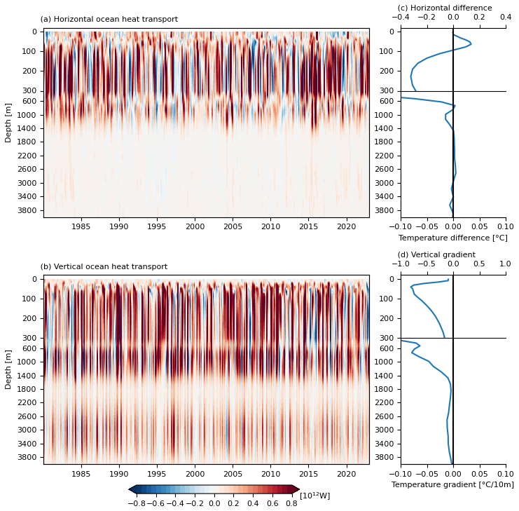
Figure 11 Vertical structure of the heat budget terms in the Cabo Verde archipelago. Horizontal (a) and vertical (b) ocean heat transport anomalies relative to the 1980–2009 daily climatology. To emphasize sustained anomalies that have a strong impact on the heat content, high-frequency variability was removed by applying a 60 d moving average. Mean (1980–2022) difference between the domain average temperature and the temperature along the boundary of the Cabo Verde archipelago region (c). Mean (1980–2022) vertical temperature gradient (d). Note the changing x-axis scaling for the top 300 m in panels (c) and (d).

Between 600 and 1000 m depth, the horizontal temperature difference reverses sign, i.e., the Cabo Verde archipelago region is warmer than the surrounding area (Fig. 11c). The temperature difference is comparably small, but the horizontal heat transport still contributes to events (Fig. 10d). Due to the reversed sign, a barotropic velocity change is expected to cause opposing heat transport anomalies between 300 and 600 m and between 600 and 1000 m depth. This is indeed often visible in Fig. 11a. As a consequence, MHWs typically do not occur at the same time.

Below 1000 m depth, the vertical transport of heat dominates the development of MHWs (Fig. 10d). Nevertheless, a break in the vertical coherence occurs around 1300 m depth, where the vertical temperature gradient becomes small as it declines towards a minimum at 1600 m (Fig. 11d). Consistently, vertical heat transport anomalies show a minimum as well (Fig. 11b). Below 2000 m, the vertical gradient and vertical heat transport increase again and lead to intermittent short MHW events (Fig. 11b, d). Different long-term temperature trends at different depths slightly modify the exact transition between the described layers of coherent MHW occurrence when the fixed_30yr baseline is used. Nevertheless, the described vertical structure of the heat budget terms remains visible (Fig. 10a, c). Note that the linear trend in temperature (and heat content) itself results from a small imbalance in the time mean fluxes shown in Fig. 11a, b.

4 Discussion and conclusion

4.1 Detecting MHWs at depth

In this study, we analyzed the characteristics of temperature extremes (MHWs) throughout the entire Atlantic Ocean. By using a hierarchy of ocean model grids, we identified the impact of the horizontal resolution, ocean dynamics and different baselines on the derived MHW statistics.

We found that interpolation of the temperature from a $\mathrm{1}/\mathrm{20}$ to a $\mathrm{1}/\mathrm{4}$° grid does not impact the derived statistics. This is important for the interpretation of model results but has further implications for the detection of MHWs from gridded observational products. The reason for this result is likely that MHWs do not occur at isolated grid points but almost always cover an area that is larger than the grid resolution of the datasets (mostly $\mathrm{1}/\mathrm{20}$ to $\mathrm{1}/\mathrm{4}$°). Thus, as long as the target grid size is still small enough to capture the typical extent of MHWs in the region, it is expected that the horizontal resolution of the temperature dataset does not affect the MHW statistics. This would also mean that the interpolation of high-resolution along-track data onto a regular, coarser grid does not impact the detection of MHWs.

However, statistics change if the horizontal resolution of the grid affects the dynamic scales resolved in a model. The coarser-resolution model with otherwise the same surface forcing and initial conditions generally overestimates the duration and underestimates the frequency and intensity of MHWs. This result is consistent with a coupled model study conducted by Pilo et al. (2019). Coarse horizontal resolution is often mentioned as a limiting factor in MHW studies (e.g., Hövel et al., 2022). In the presence of highly variable currents and at mid-depths (100–3000 m), differences between the high- and coarse-resolution configurations can be substantial. This means that studying the impact of MHWs on deep ecosystems requires models with sufficiently high resolution, in particular along the continental slopes. Differences are overall small at the surface, except for the Gulf Stream and North Atlantic Current (NAC) regions, but the discrepancy is expected to be larger for coarser $\mathrm{1}/\mathrm{2}$ and 1° models (Pilo et al., 2019).

While Hobday et al. (2016) mention that the horizontal and temporal resolution of the temperature dataset are important, we argue that the horizontal resolution (in certain limits that are probably related to the typical extent of MHWs) plays a minor role, as long as the dynamics represented in the dataset are the same. This is highly advantageous because MHWs can be detected equivalently on the native model grid without interpolation or at a coarser resolution, whichever option is less computationally expensive. This simplifies the comparison of different satellite products and models. As a result, the applied two-way nesting provided a convenient tool to produce a manageable dataset containing mesoscale effects. The computational resources needed for this study would have been much higher if MHWs had to be detected on the high-resolution grid. Detecting MHWs on the high-resolution grid requires approximately 25 times more computing time and significantly more resources for analysis and storage. Daily MHW statistics for 43 years at all 46 depth levels on the coarse grid (only the domain covered by the nest) take up 90 GB of storage, whereas it is 700 GB on the high-resolution grid. The amount of data that needs to be processed is even higher, as the output file size is strongly reduced by compression.

The choice of a suitable baseline is widely discussed in the current literature and depends on the scientific question (Amaya et al., 2023b; Smith et al., 2025). Modeled temperature trends can strongly differ across experiments, for example, dependent on the time of the model spin-up (adjustment from initial conditions). While trends are robust in approximately the top 100 m, they strongly change with the model's spin-up time at greater depths. Trends at depth vary in magnitude and even have opposite signs in our model experiments that just differ in the initial conditions. As a consequence, fixed baselines (e.g., the fixed_30yr and fixed_43yr baselines used here) do not yield reasonable results below approximately 100 m depth in the presence of model drift. Instead, MHW statistics are dominated by trends that arise from the models' adjustment from the initial conditions rather than trends related to the surface forcing or intrinsic oceanic variability. The choice of the baseline is then not only a question of interpretation, but the slow adjustment of the deep circulation does not allow for any meaningful interpretation of the results. We have investigated this in only one model configuration here, but model drift is common to nearly all forced and coupled models (e.g., Tsujino et al., 2020). As a consequence, if the aim is to include multi-decadal trends in the MHW statistics beyond approximately 100 m depth, a model spin-up with sufficient time to allow the sub-surface to equilibrate is needed. It is not possible to provide a universally applicable recommendation on the exact spin-up time or procedure. We have tested only the spin-up strategy recommended by the OMIP-2 protocol (Tsujino et al., 2020), but other strategies exist as well. Still, our results show that the required spin-up time will depend on the depth. For the surface, it was shown that a 22-year-long spin-up (1958–1980 in the first cycle) is sufficient. Mid-depth water masses do not show a strong temperature drift after the second cycle (124 years; not shown), while abyssal water masses at depths beyond 5000 m have not fully adjusted even after 300 years of spin-up. Therefore, studies that focus on near-surface MHWs get away with using a short spin-up of only a few years, as the ocean model typically stabilizes quickly. Studies that focus on the deeper ocean will need a much longer spin-up time, with probably more than 300 years for abyssal basins. Such long spin-ups are often not feasible at the resolution used in this study. Additional constraints to reduce model drift, such as the assimilation of observations, could also alleviate the problem while, at the same time, acknowledging the fact that deep observations are sparse. Ocean reanalysis was successfully used by Fragkopoulou et al. (2023) to study MHWs at depth. Nevertheless, frequent and widespread observations typically exist only in the top 1000 m, and thus also reanalysis products should be treated with caution in the deep ocean. Furthermore, a downside of many assimilation techniques, in particular of nudging, is that they may violate conservation laws (Zeng and Janjić, 2016; Janjić et al., 2014), and thus studying the drivers of MHWs is problematic in such datasets due to spurious sources and sinks of heat. With a detrended baseline, statistics are not identical but similar in the presence (first cycle) and absence (sixth cycle) of model drift. Studies applying a detrended baseline to focus on interannual to decadal variability are therefore possible with a relatively short model spin-up (roughly 20 years) as well.

4.2 Characteristics, drivers and trends

From their definition, it immediately follows that MHWs need to occur everywhere (disregarding the condition that the temperature threshold must be exceeded for 5 consecutive days). Therefore, the pure observation that MHWs occur throughout the entire water column is not surprising. Still, the detection of MHWs is a useful tool to comprehensively study the characteristics of temperature variability and how it changes in time. In the upper ocean, the temperature is highly variable (large variance), and anomalously high temperatures occur for relatively short times. In the deep ocean, temperature anomalies associated with MHWs are smaller and occur on longer timescales compared to the surface. Along the continental slope, MHWs with maximum intensities on the order of 1 °C do occur. Given that the temperature tolerance of deep-sea species like cold-water corals is expected to be around 4 °C (Morato et al., 2020), this could have major impacts for ecosystems that are already close to their upper temperature limit. In the abyssal ocean, MHW intensities do not exceed 0.1 °C. Whether such low temperature variations have any impact is yet to be investigated. In general, even small temperature anomalies could have an impact if they are sustained for sufficiently long times. At the same time, ecosystems may have adapted to large temperature variability in regions where MHWs occur very frequently and thus do not represent rare events. The aim of this study is to provide a comprehensive understanding about the characteristics of temperature variability throughout the entire Atlantic, which, when combined with biological information, will help to identify deep ecosystems that may be vulnerable to MHWs and changes in their characteristics.

Overall, our results highlight the importance of the ocean circulation for the development and characteristics of MHWs. By comparing two model configurations that differ only by their horizontal resolution, we find that mesoscale dynamics change the frequency, duration and maximum intensity of MHWs, in particular at depth. In agreement with Großelindemann et al. (2022), Zhang et al. (2023), Elzahaby and Schaeffer (2019), Wyatt et al. (2023) and Wu and He (2024), this is partly caused by mesoscale features such as eddies and meanders themselves. Additionally, indirect effects, such as changes in current structure, strength, mixed layer dynamics, and vertical as well as horizontal temperature gradients, contribute to differences between the eddy-permitting and eddy-rich configurations in our study. Highly variable currents, such as the NAC and DWBC, are related to the occurrence of short but frequent MHWs, in agreement with Fragkopoulou et al. (2023). Deep convection in the Labrador Sea and upwelling were found to strongly influence the occurrence and characteristics of MHWs at depth. Additionally, strong vertical temperature gradients at mid-depth (300–1500 m depth), for example, between warm Mediterranean Outflow Water and colder North Atlantic Deep Water, lead to regionally more intense MHWs. These MHWs are not necessarily caused by variability in the properties of the water masses themselves but rather by a vertical displacement of isotherms through internal waves or wind-driven up-/downwelling. The pronounced differences between the configurations, despite using the same atmospheric forcing, points to a major influence of ocean dynamics on the characteristics of MHWs.

In both model experiments (VIKING20X-1st and VIKING20X-6th) analyzed here, the impact of the local surface forcing on MHWs is limited to approximately the top 100 m throughout the Atlantic, with some minor regional differences. Consistent with other studies (Xu et al., 2022; Oliver et al., 2018; Chiswell, 2022), we find a positive trend in all MHW characteristics when applying a fixed baseline at the surface. Although not related to the surface forcing but rather changes in ocean dynamics, positive trends can be seen in most regions until a depth of roughly 1000 m. Between 1000 and 4000 m, negative trends prevail in the model. Although model trends are always connected to a large uncertainty, in particular in the deep ocean, this result suggests that many deep ecosystems experienced a decrease in frequency, duration and intensity of MHWs over time. At the very least, the model shows that even though trends are clearly positive at the surface, it cannot be expected that marine heatwaves increased over time throughout the water column.

A detailed study of MHWs in the Cabo Verde archipelago shows that the depth of the mixed layer marks a transition zone for both the long-term trend and variability on shorter timescales. MHWs in the mixed layer are almost exclusively driven by the surface heat flux. Consistent with results obtained by Scannell et al. (2020) and Amaya et al. (2023a), MHWs within and below the mixed layer have very different characteristics. In agreement with these studies, surface-forced MHWs can be detrained from the seasonally varying mixed layer. If they are subducted below the annual maximum mixed layer, they can persist for several years, while MHWs closer to the surface are typically much shorter.

Below approximately 100–300 m depth, the surface forcing does not affect MHWs in the Cabo Verde archipelago. Instead, vertical and horizontal ocean heat transport anomalies drive MHWs. While MHWs are detected independently at each model level, coherent vertical changes in heat content lead to vertically coherent MHWs. Depth levels that show coherent MHW events are mostly independent of the baseline used and span depth ranges of a few hundred to 1000 m. The vertical extent of these depth ranges can be directly linked to the vertical structure of the MHWs' physical drivers.

Below the mixed layer and above 1000 m depth, horizontal and vertical heat transport both contribute to MHWs. In deeper layers, slow horizontal currents and a vanishing horizontal temperature gradient lead to dominance of the vertical transport. Different temperature trends at different depths can slightly modify the depth ranges in which MHWs occur coherently. Nevertheless, the impact of changing ocean heat transports on shorter timescales is apparent for both the detrended and fixed_30yr baselines. It is important to note that the described processes (e.g., changes in the vertical heat transport) act over the entire archipelago and are not related to processes that occur along the island slopes, for example.

Although this detailed analysis was carried out only for the Cabo Verde archipelago, the Atlantic-wide statistics suggest that similar mechanisms occur throughout most of the basin. As a result, our study strongly supports the conclusions of Sun et al. (2023), Zhang et al. (2023), Elzahaby and Schaeffer (2019), Schaeffer and Roughan (2017) and Wyatt et al. (2023) that measuring temperature at the surface alone yields no information on extreme temperature events below the mixed layer. Conversely, studying MHWs at depth will require detailed knowledge of ocean dynamics. This includes vertical velocities that are very small compared to horizontal velocities but can be very important due to larger vertical than horizontal temperature gradients.

In conclusion, this study presents results of a single model simulation, but the main results are consistent with various other publications as described above (e.g., Fragkopoulou et al., 2023; Wu and He, 2024; Großelindemann et al., 2022). The mean characteristics at the surface and at depth are qualitatively and quantitatively similar to the ocean reanalysis-based study of Fragkopoulou et al. (2023). As direct observations for a larger domain at daily resolution are not available below the surface, studies of MHWs at depth will have to rely on models in the foreseeable future. This study provides valuable information about the characteristics of MHWs at depth and how they are related to ocean dynamics, as well as on potential challenges when detecting deep MHWs in models. Additionally, it provides a unique dataset to launch investigations on the impact of MHWs on sub-surface ecosystems.

Appendix A

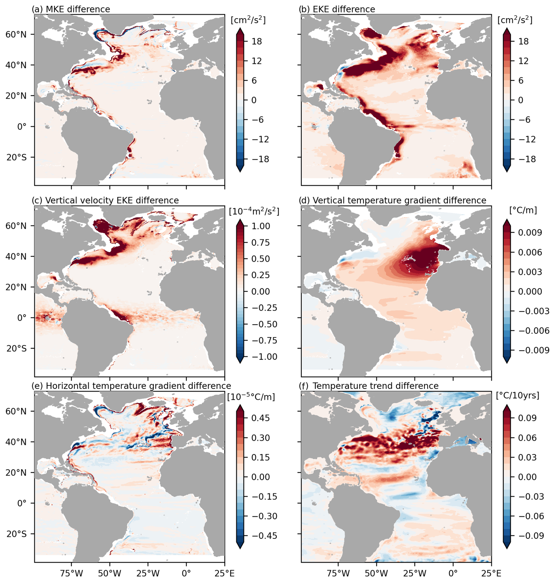
Figure A1 Differences between the coarser-resolution ORCA025 and high-resolution VIKING20X configurations. Mean kinetic energy (a), eddy kinetic energy (b), eddy kinetic energy of the vertical velocity (c), vertical temperature gradient (d) and horizontal temperature gradient (e). All maps show the difference between the mean quantities (1980–2022). The temperature trend (linear regression slope) difference in panel (f) is based on the same time period.