Statistical analysis of ocean currents in the eastern Mediterranean

We examine the probability density function (pdf) of current speeds at the DeepLev station located in the eastern Mediterranean Sea near the central coast of Israel. The currents cover depths from the surface to over 1.3 km and span a period from November 2016 to March 2024. We estimate the parameters of three typical distributions that are usually used to model the pdfs of currents and wind speed: the Weibull, the general extreme value, and the generalized gamma. We find that the three-parameter generalized gamma distribution best describes the pdfs of the observed current-speed series. Still, the studied current-speed time series may not be long enough to assess the exact values of the underlying pdf as some years exhibit stronger currents that affect the distribution. We also study the time series of the difference between consecutive current speeds and find that the stretched exponential pdf describes better (than the normal distribution) their statistics. The comparison of the measured current-speed pdfs to current-speed pdfs of a high-resolution (1 km) regional circulation model (ROMS) and Copernicus Mediterranean reanalysis daily mean currents (∼ 4.6 km resolution) indicates discrepancies from the data. Our results may help to improve statistical models for ocean currents and the estimation of extreme current events.

1 Introduction

The circulation of the ocean is a vital player in the climate system. It helps to regulate the climate system and is linked to far-reaching teleconnections. Ocean circulation played a significant role in past climate events and is expected to continue to do so in the changing climate of the future. The ocean's circulation and dynamics are driven by various sources, including surface winds, tides, and pressure gradients, which are also influenced by local temperature and salinity.

Various classical theories explain the characteristics and existence of ocean currents. These include the Ekman layer theory (Ekman, 1905) that describes the impact of winds on surface currents, the theories for western boundary currents (Stommel, 1948; Munk, 1950), and the Stommel–Aron theory (Stommel and Arons, 1960) that explains the abyssal ocean circulation. However, since winds and currents are stochastic in nature (e.g., Seguro and Lambert, 2000; Chu, 2008a), they require statistical analysis and formulation. Indeed, many studies have performed statistical analyses of ocean currents and proposed statistical models to explain their observed statistical properties.

Being a main forcing of ocean currents and easier to observe, numerous studies have focused on investigating the statistical distribution of winds (e.g., Seguro and Lambert, 2000; Monahan, 2006a, b; Campisi-Pinto et al., 2020; Justus et al., 1978; Takle and Brown, 1978; Bowden et al., 1983; Conradsen et al., 1984; Troen and Petersen, 1989; Lun and Lam, 2000; Ulgen and Hepbasli, 2002; Monahan, 2006a, b; Carta et al., 2009; Kiss and Jánosi, 2008; Kelly et al., 2014; Drobinski et al., 2015), while less attention has been given to the statistical properties and distribution of ocean currents (Chu, 2008a, b; Ashkenazy and Gildor, 2011; Ashkenazy et al., 2016; Campisi-Pinto et al., 2020). Most of these studies concluded that the winds and currents follow the Weibull distribution (Justus et al., 1978; Takle and Brown, 1978; Bowden et al., 1983; Conradsen et al., 1984; Troen and Petersen, 1989; Lun and Lam, 2000; Seguro and Lambert, 2000; Ulgen and Hepbasli, 2002; Chu, 2008b; Manwell et al., 2010; Kelly et al., 2014). Yet, other studies used other distributions to model wind and current-speed data (Tuller and Brett, 1984; Bauer, 1996; Carta and Ramirez, 2007; Morrissey and Greene, 2012; Bel and Ashkenazy, 2013; Campisi-Pinto et al., 2020).

Studying the statistical properties of ocean currents is essential for enhancing our understanding and modeling of ocean dynamics and for estimating the likelihood of rare current events. In addition, for devising better parameterizations for subgrid mixing, one should understand the velocity distribution and its relation to the various forcing of surface ocean circulation. This knowledge also supports the effective management and protection of marine ecosystems and is critical for the safe and efficient design of offshore structures. Since the statistical behavior of ocean currents varies across different regions (see more details below), our focus on the currents of the eastern Mediterranean will contribute insights into and improve the modeling of this area.

The pdfs of upper-ocean currents are influenced by the statistical properties of wind stress (e.g., Chu, 2008b, 2009; Ashkenazy et al., 2015). In particular, resonance between wind stress and the Coriolis force (the inertial frequency) – often referred to as the “chimney effect” – can significantly impact ocean currents and their statistical characteristics, even at considerable depths (Lee and Niiler, 1998; Alford et al., 2016); we note that the inertial frequency is dominant in our current records (Solodoch et al., 2023). Additionally, other factors such as density-driven currents (convection), bathymetry, tides, and persistent mesoscale eddies can also affect the statistical properties of ocean currents. Among these, long-lived eddies may be especially relevant in our region of study.

Previous studies investigated the probability distribution of surface geostrophic current speed based on satellite altimetry data and found that these are Weibull distributed where different parts of the world ocean are characterized by different values of the shape and scale parameters (Smith and Gille, 1998; Chu, 2008b, 2009). Chu (2008a) analyzed the speed of the upper levels of the tropical Pacific Ocean and found that it follows the Weibull distribution within the top 50 m. However, the distribution was found to be different at deeper levels. The same study also discovered that the parameters of the Weibull distribution change during El Niño and La Niña events. The statistics of the global ocean surface currents that were estimated based on altimetry data were analyzed using surrogate data tests; it was found that the generalized gamma (GG) distribution (a generalization of the Weibull distribution) better fits the probability distribution of the data (Campisi-Pinto et al., 2020).

In addition to the analysis of current speeds, previous studies have also examined the statistics of velocity components of surface currents (rather than current speed) based on altimetry data. It has been found that the distribution of the velocity components differs depending on the size of the ocean area being examined (Smith and Gille, 1998; Gille and Smith, 2000). When focusing on small ocean areas, the distribution appears to follow a Gaussian distribution, whereas when considering the mean currents over extensive ocean areas, the probability appears to be an exponential distribution.

Coastal ocean dynamics application radar (CODAR) systems can estimate surface currents with high accuracy in both time (30 min–1 h) and space (ranging from hundreds of meters to several kilometers). Laws et al. (2010) presented the probability distribution of these current velocities but did not discuss the theoretical distribution that corresponds to these currents. CODAR-based surface current speeds at the Gulf of Eilat/Aqaba were estimated to follow the Weibull distribution (Ashkenazy and Gildor, 2011). This study introduced an Ekman layer model forced by local winds and additional stochastic geostrophic currents to reproduce the observed surface current pdf. It was also found that the spatial variability of the shape parameter of the Weibull distribution is larger in the Gulf of Eilat in comparison to the Nan Wan Bay in Taiwan (Ashkenazy et al., 2016). Kabir et al. (2015) used the HYbrid Coordinate Ocean Model (HYCOM) and high-frequency radar data to study the statistics of the Gulf Stream current and concluded that the Weibull distribution underlies the current-speed distribution.

The statistics of sub-surface and deep-ocean currents received less attention than the surface currents. This is mainly due to the lack of long, continuous, measured ocean currents. Paquette (1972) analyzed a series of relatively short-time current data from various depths and locations and found that the logarithm of the current speed is approximately normally distributed. Chu (2008a) studied the current-speed distribution of the tropical Pacific and found that the currents in the upper 50 m follow the Weibull distribution unlike the deeper currents of 100 to 200 m. Another study (Bracco et al., 2000a) used barotropic ocean turbulence numerical simulations to investigate the velocity distribution inside and outside coherent structures. These authors also used observations (Bracco et al., 2000b) and numerical simulations (Bracco et al., 2003) of the North Atlantic to study the probability distribution of the Lagrangian current and found that the velocity components do not follow the Gaussian distribution but the exponential distribution; this finding may have implications on the parameterization of particle dispersion.

The present study aims to investigate the statistical characteristics of the current-speed time series and to deduce the pdf associated with these time series. Our analysis is based on data collected over 7 years of current meter deployment in a mooring site (named DeepLev) in the Levantine basin of the east Mediterranean Sea) at the foot of the continental slope offshore Israel (Katz et al., 2020); see Fig. 1. We find that among the Weibull distribution, the general extreme value (GEV) distribution, and the generalized gamma (GG) distribution, the final is the best for modeling the statistics of the current speeds. We also analyzed the statistics of current-speed increments and found that the stretched exponential distribution better fits the data than the normal distribution. The analysis of the currents of high-resolution oceanic general circulation (OGCM) simulations of the Mediterranean Sea (Solodoch et al., 2023) and Copernicus oceanic reanalysis (Escudier et al., 2020) indicates differences from the data.

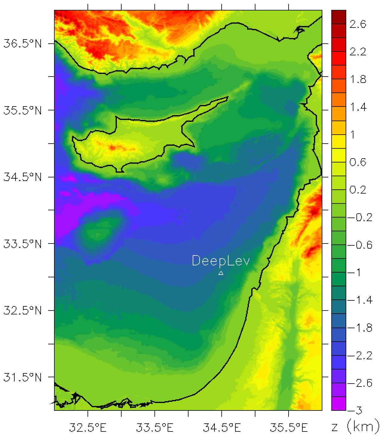
Figure 1 Bathymetric map of Israeli waters and the greater Levant region. The location of the DeepLev station is indicated by the white triangle. The black contour line indicates the coastline.

Below we first describe the data and methods used in this study (Sect. 2). We then present the results (Sect. 3) and provide a summary and conclusions (Sect. 4).

2 Data and methods

2.1 Studied area and data

The circulation of the Mediterranean Sea has been studied extensively in the past few decades (e.g., Malanotte-Rizzoli et al., 2014, and references therein). The Mediterranean Sea is connected to the global ocean (Atlantic Ocean) through the Straits of Gibraltar, where relatively cold and fresh water flow to the Mediterranean Sea at the surface layer. This water becomes warmer, saltier, and heavier while flowing along the southern coast of the Mediterranean Sea to the Levantine basin and the eastern part of the Mediterranean Sea; the Levantine surface water is warmer by 3–4 °C (Shaltout and Omstedt, 2014) and saltier by ∼ 16 ppt (Ferguson et al., 2008) than the water entering the Gibraltar Straits. Then the water completes the circulation back to the Gibraltar Straits through intermediate water levels along the northern parts of the Mediterranean Sea and exits back to the Atlantic Ocean through the lower parts of the Gibraltar Straits (Bergamasco and Malanotte-Rizzoli, 2010; Tanhua et al., 2013; Malanotte-Rizzoli et al., 2014). The deep-water formation in the Mediterranean Sea exhibited drastic and rapid changes (the Eastern Mediterranean Transient) (Roether et al., 1996) and was studied using observation and models (e.g., Ashkenazy et al., 2012; Malanotte-Rizzoli et al., 2014; Amitai et al., 2017, 2019; Mavropoulou et al., 2022; Parras-Berrocal et al., 2022, 2023; Pinardi et al., 2023).

A deep-water mooring, the DeepLev, was recently installed in the Levantine Basin of the eastern Mediterranean (Katz et al., 2020). The mooring location is about 50 km offshore of Haifa (Israel), at a depth of 1.5 km; its coordinates are 33.0618° N, 34.4888° E. The DeepLev mooring was used to gather data about the water's physical, chemical, and biological properties at different depths, as well as sediment transport. These measurements were taken from November 2016 onward. In this study, we focus on the current measurements of the DeepLev.

DeepLev data were used to study several aspects of ocean dynamics in the eastern Mediterranean Sea. Katz et al. (2020) described the data collected at the DeepLev mooring and also estimated the sedimentation flux at this region. This study concluded that continental sediment can reach distances farther than 100 km offshore. Another study (Feliks et al., 2022) analyzed the DeepLev current velocity and found upper-ocean oscillations that are much stronger and much slower than the tidal oscillations. DeepLev current and pressure data were also used to study tidal variability in this region (Mantel et al., 2024). It was found that the semi-diurnal and diurnal tides vary seasonally. An additional study (Haim et al., 2024) used the DeepLev mooring station to measure surface wave patterns and dynamics. A recent modeling study of the eastern Mediterranean Sea compared velocity spectra from DeepLev to the model's simulations (Solodoch et al., 2023).

We consider the DeepLev current velocity measured by Acoustic Doppler Current Profilers (ADCPs), which were mounted at depths of 30, 100, and 400 m. From these ADCPs, we analyzed the current velocities of depths of 10, 45, 80, 160, and 430 m. In addition, we used a single-point current measurement at a depth of 1300 m. For more details on the instruments, see Table 1 of Katz et al. (2020). The selected depths roughly represent the different parts of the water column: the mixed layer, the thermocline, and the deep ocean. The data we analyzed cover the time period from 14 November 2016 to 5 March 2024. Data were collected through nine consecutive deployments. In two deployments, the 10 m instrument failed, and in one deployment, the instrument intended for 1300 m depth was placed at a depth of 800 m and thus is ignored here. These gaps and the gaps between the different deployments were ignored in the statistical analysis. The different instruments were recorded using different sampling rates during the different deployments, and we resampled them to the longest sampling time of 2 h.

In addition to the analysis of the measured data, we also analyzed the currents of a state-of-the-art oceanic general circulation model (Solodoch et al., 2023). We analyze the model's currents to verify the ability of the model to reproduce the statistical properties of the observed currents. Such a comparison may help to improve the performance of the model, eventually leading to better prediction and understanding of the ocean dynamics. Solodoch et al. (2023) used the Coastal and Regional Ocean Community (CROCO) model (Debreu et al., 2012) that is based on the Regional Oceanic Modeling System (ROMS) (Shchepetkin and McWilliams, 2005). The model was forced by realistic atmospheric fields and reanalysis currents (Escudier et al., 2020) that were used to simulate the time period between 2017 and 2019 using 3 km spatial resolution, the time period between February 2017 to December 2018 using 1 km resolution, and the winter and summer of 2018 using 300 m resolution. For a comparison between DeepLev velocity spectra and the model, see Solodoch et al. (2023). Below, we focus on the 1 km model simulation as this simulation has both a fine resolution and long simulation time; unfortunately, the CROCO simulations are highly time-consuming such that we were unable to simulate the entire time of the DeepLev measured data. The temporal resolution of the 1 km resolution data is 2 h, the same as the resampling rate of the data.

The simulation described in the previous paragraph does not span the temporal extent of the measured DeepLev data. We thus also analyzed the Copernicus Marine Environment Monitoring Service (CMEMS) reanalysis data (Escudier et al., 2020). We consider the same time period as the observed data (14 November 2016 to 5 March 2024); the Copernicus currents are daily average, and we thus used the daily mean current speed of the data to compare the two.

2.2 Methods

In this study, we examine three pdfs, the Weibull, the general extreme value (GEV), and generalized gamma (GG) distributions, as possible statistical distributions of current speeds.

The Weibull distribution is a two-parameter pdf defined as

$$\begin{array}{}\text{(1)}& f(x>\mathrm{0})={\displaystyle \frac{k}{\mathit{\lambda }}}{\left({\displaystyle \frac{x}{\mathit{\lambda }}}\right)}^{k-\mathrm{1}}{e}^{-(x/\mathit{\lambda }{)}^k},\end{array}$$

where λ is the scale parameter (here has units of speed) and k is the (dimensionless) shape parameter. k=1 reduces the Weibull distribution to the exponential distribution, while k=2 reduces the Weibull distribution to the Rayleigh distribution.

The GEV distribution is a three-parameter pdf defined as

$$\begin{array}{}\text{(2)}& f\left(x\right)={\displaystyle \frac{\mathrm{1}}{\mathit{\sigma }}}t(x{)}^{k+\mathrm{1}}{e}^{-t\left(x\right)},\end{array}$$

where

$$\begin{array}{}\text{(3)}& t\left(x\right)=\left\{\begin{array}{ll}{\left(\mathrm{1}+k\left(\frac{x-\mathit{\mu }}{\mathit{\sigma }}\right)\right)}^{-\mathrm{1}/k}& \mathrm{if}k\ne \mathrm{0},\\ e^{-(x-\mathit{\mu })/\mathit{\sigma }}& \mathrm{if}k=\mathrm{0},\end{array}\right.\end{array}$$

while μ is the location parameter, σ is the scale parameter, and k is the shape parameter; in this study, the units of μ and σ are units of speed, while k is dimensionless. The GEV distribution is the general pdf in extreme value theory and may be reduced to the Fréchet, Weibull, and Gumbel pdfs under appropriate assumptions.

The GG distribution is a three-parameter pdf defined as

$$\begin{array}{}\text{(4)}& f(x>\mathrm{0})={\displaystyle \frac{\mathrm{1}}{\mathrm{\Gamma }\left(\mathit{\epsilon }\right)}}{\displaystyle \frac{k}{\mathit{\lambda }}}{\left({\displaystyle \frac{x}{\mathit{\lambda }}}\right)}^{\mathit{\epsilon }k-\mathrm{1}}{e}^{-(x/\mathit{\lambda }{)}^k},\end{array}$$

where Γ is the gamma function, λ is the scale parameter (here with speed units), and k and ε are the dimensionless shape parameters. The GG pdf reduces to the Weibull pdf when ε=1. We use the maximum likelihood method to fit the theoretical pdf (model) to the data.

In addition to the above three pdfs, we used the normal and stretched exponential (or the generalized normal distribution) pdfs to model the current-speed increment time series. The normal distribution is defined as

$$\begin{array}{}\text{(5)}& f\left(x\right)={\displaystyle \frac{\mathrm{1}}{\sqrt{\mathrm{2}\mathit{\pi }}\mathit{\sigma }}}{e}^{-\frac{x^{\mathrm{2}}}{\mathrm{2}{\mathit{\sigma }}^{\mathrm{2}}}},\end{array}$$

where σ² is the variance of the distribution. The location parameter of the normal distribution (the mean) μ is not included here as the current-speed increment time series are stationary and the mean of the distribution is very close to zero. The stretched exponential (generalized normal distribution) pdf is defined as

$$\begin{array}{}\text{(6)}& {\displaystyle \frac{\mathrm{1}}{\mathrm{2}\mathit{\sigma }\mathrm{\Gamma }\left(\mathrm{1}+\frac{\mathrm{1}}{\mathit{\beta }}\right)}}{e}^{-|\frac{x}{\mathit{\sigma }}{|}^{\mathit{\beta }}},\end{array}$$

where σ is the scale parameter and β is the shape parameter. The stretched exponential pdf takes the form of the exponential pdf when β=1 and the form of the normal pdf when β=2.

We examine here two- and three-parameter pdfs, and it is necessary to determine, for example, whether the two-parameter Weibull pdf exhibits similar performance as the three-parameter pdf or not. Naturally, one expects the three-parameter pdf to yield a better fit to the observed distribution simply since it has one additional parameter. The likelihood ratio test (Davidson and MacKinnon, 2004) aims to determine whether the more complex pdf, which has more parameters, significantly outperforms the fit to the histogram of the data when using the simpler pdf with fewer parameters. In other words, the likelihood ratio test determines whether the data significantly favor the pdf with the more parameters in comparison to the fewer-parameter pdf. The likelihood ratio test may be applied when the pdf with the fewer parameters is a subset of the pdf that has more parameters. We use this test to verify whether the GG pdf exhibits a significantly better fit than the Weibull pdf.

In addition to the likelihood ratio test, we quantify the difference Δ between the distribution of the data and the pdf of the theoretical pdfs by calculating the square root of the mean of the square of the difference between the distribution of the data and the fitted pdf. To examine more precisely the tail of the distribution, we repeated the analysis after taking the log of the pdf. Smaller Δ values indicate a better fit of the theoretical pdf to the observed one.

3 Results

3.1 Measured currents

The current-speed time series analyzed here are presented in Fig. 2. We first note that there are gaps in the data; these gaps are due to the lapse between the different deployments and due to errors or instrument failures in some deployments (in two deployments for the 10 m depth instrument and in one deployment for the 1300 m depth instrument). The current time series of the upper four depths exhibit similar behavior with a “noisy” pattern superimposed on slow modulations. The slow modulations seem to be associated with winter storms, which extend well below the mixed layer (see Fig. 7c of Solodoch et al., 2023, for the depth of the mixed layer). The slow modulations are less evident in the deeper stations of depths of 430 and 1300 m. As expected, the mean and the standard deviation of the current series decrease with depth. We present the correlation between the time series of the different depths in Fig. 3. This figure shows that the correlation between the time series of the different depths is significant (Fig. 3b). As expected, the correlation decreases when the depth distance becomes larger (Fig. 3c, d). Moreover, the correlation decreases with time lag slowly (tens of days; Fig. 3b), indicating that the current-speed time series exhibits slow modulations, possibly due to seasonal effects or mesoscale eddies. The correlation between the surface current and the deep ocean suggests energy injection from the surface.

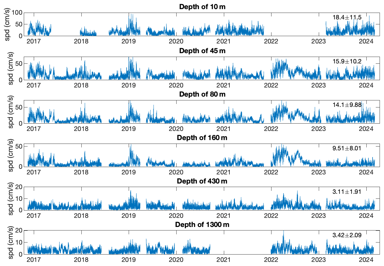
Figure 2 The measured current-speed (in cm s⁻¹) time series for the different depths analyzed here. The numbers in the top-right corner of each panel indicate the mean ± SD. Note that the ordinate axes have different ranges in different panels.

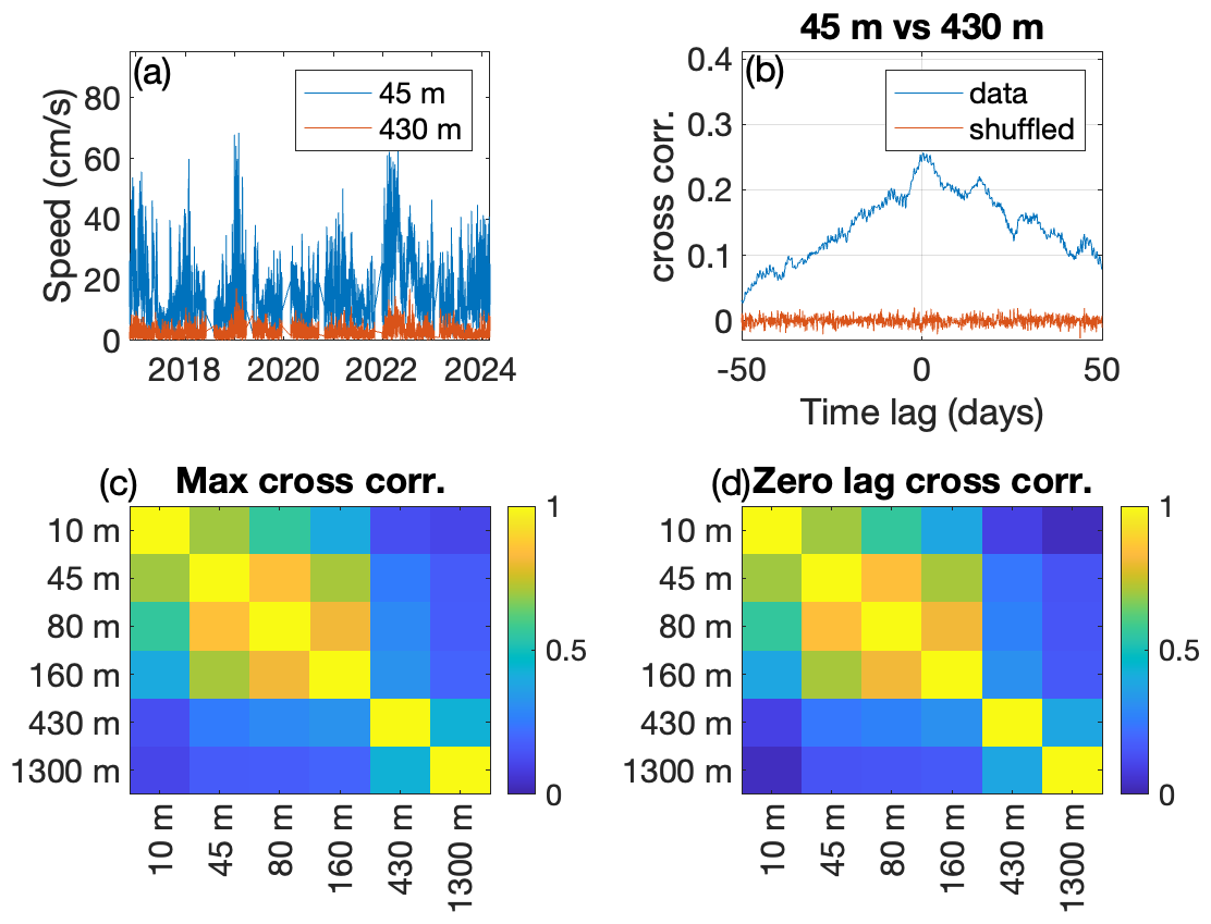
Figure 3 (a) The current time series of 45 m (blue) and 430 m (red) as a function of time. (b) The cross-correlation function between the two time series shown in blue as a function of time lag (in days). The red time series depicts the time cross-correlation of the shuffled time series (red). (c) The maximum cross-correlation between the time series of the different depths. (d) The zero-lag cross-correlation between the time series of the different depths. Note the similarity to panel (c).

Next, we construct the pdf of the current-speed time series of the different depths. These are plotted in Fig. 4 in both regular (left panels) and semi-log (right panels) plots. The latter aim to emphasize the tail of the distribution, which presents information regarding extreme current-speed events. We fitted the Weibull, GEV, and GG pdfs to the observed distributions. The three-parameter GEV and GG pdfs seem to exhibit a better fit than the two-parameter Weibull pdf; for both the central part of the distribution and the tails, the Weibull pdf falls below the observed distribution as well as below the pdfs of the two other three-parameter pdfs. We will quantify the performance of the different pdfs below. When focusing on the right tail of the distribution, it is apparent that the GG distribution exhibits the best fit to the data, and it is situated between the lower estimate of the Weibull distribution and the upper estimate of the GEV distribution.

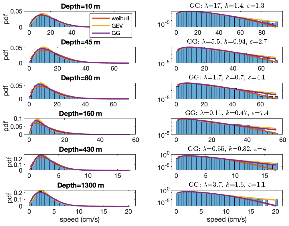
Figure 4 The pdfs of the current-speed time series shown in Fig. 2 in regular (left panels) and semi-log (right panels) plots. The corresponding depths are indicated in the title of the left panels, whereas the parameters of the fitted generalized gamma (GG) pdf are indicated in the title of the right panels. The fitted Weibull (red), GEV (yellow), and GG (purple) pdfs are also included.

We summarize the parameters of the three fitted pdfs in Fig. 5; the fitted parameters of the data are represented by the blue circles. The λ parameter of the Weibull distribution is the scale parameter and, as expected, decreases with depth, similarly to the mean current speed. The k shape parameter of the Weibull distribution is less than 1.8 and larger than 1.3, indicating that the tail of the distribution decays faster than exponential decay.

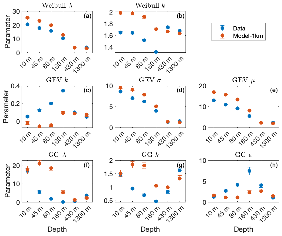
Figure 5 The estimated pdf parameters versus the depth of the data (blue circles) and 1 km resolution model (red circles) for the Weibull (a, b), GEV (c, d, e), and GG (f, g, h) distributions. The error bars indicate the 5 %–95 % confidence interval (which is not always visible). The estimated GG parameters for the data at depths of 80 and 160 m (represented by the blue circles in the bottom panels) are less accurate as the maximum likelihood estimation (MLE) did not converge.

The second row of Fig. 5 displays the GEV distribution parameters; the parameters of the data are indicated by the blue circles. μ and σ are the location and scale parameters and decrease with depth, similarly to the mean and SD of the data (included at the top-left corner of the panels of Fig. 2). The k parameter is positive and smaller than 0.4. Larger k values indicate slower decay of the tail of the distribution.

The fitted parameters of the GG distribution are summarized in the third row of Fig. 5 (blue circles); see also the titles of the right column panels of Fig. 4. Here, the scale parameter λ does not always reflect the decrease in the mean current speed with depth. The k shape parameter exhibits much smaller variability ($\mathrm{0.5}\lesssim k\lesssim \mathrm{1.8}$) in comparison to ε ($\mathrm{0}<\mathit{\epsilon }<\mathrm{8}$). Such a larger range of ε indicates that the observed pdf exhibits considerable irregularities. This is also expressed in the interannual variability of the estimated GG parameter; see Fig. A13. Interestingly, the shape parameters of all the distributions (k and ε) change monotonically from the surface to a depth of 160 m, but their trend is reversed between the depths of 430 and 1300 m.

We next examine whether the three-parameter GG pdf better models the current-speed data in comparison to the two-parameter Weibull pdf. These two pdfs are nested; i.e., the GG pdf reduces to the Weibull pdf when ε=1. For this purpose, we use the likelihood ratio test. We find, for all depths except the deepest location, that the null hypothesis is rejected such that the GG pdf provides a better description of the data; for the deepest location, the Weibull and GG pdfs exhibit a similar fit (see Fig. 4), and the null hypothesis that the pdfs are similar is not rejected. We thus conclude that GG pdf more correctly models the current-speed statistics.

We next present the results of another test that quantifies the performance of the fitted pdfs. As described in Sect. 2, we calculate the Δ measure (i.e., the square root of the sum of the square difference), based on the observed and the fitted pdfs, on both regular and semi-log plots. The results are depicted in the top panels of Fig. 6, where the left panel plots the Δ values that are based on a regular plot and the right panel shows the Δ values that are calculated based on a semi-log plot. A smaller Δ indicates a better fit of the proposed pdfs. We obtain the smallest Δ for the GG pdf (yellow circles) for almost all depths when calculated using a regular plot. On semi-log scales, however, the results are more complex, where both the GG and GEV pdfs seem to be acceptable models for the tail of the distributions. Overall, our results suggest that the GG pdf is the best pdf (among the three studied here) to model the current-speed pdfs at all depths.

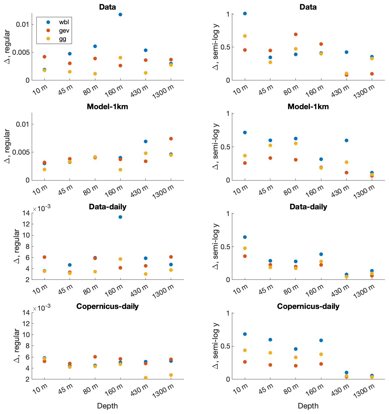
Figure 6 The depth dependence of the difference measure Δ, i.e., the difference between the observed and fitted distributions for the measured data (upper panels), 1 km resolution model (second-row panels), daily mean measured currents (third-row panels), and Copernicus daily mean reanalysis (bottom panels). Presented are the results for the fit to the Weibull (WBL, blue), GEV (red), and GG (yellow) distributions calculated based on regular (left panels) and semi-log (right panels) pdfs.

3.2 1 km resolution model

As mentioned in Sect. 2, Solodoch et al. (2023) performed state-of-the-art simulations of the eastern Mediterranean Sea, spanning the initial part of the DeepLev measurements. The simulated current time series are plotted in Fig. A1 and exhibit a smoother pattern than the measured currents shown in Fig. 2. These different patterns result in current distributions (Fig. A2) that are different than the observations (Fig. 4). This difference is expressed by the different values of the fitted parameters of the model (red circles in Fig. 5) in comparison to those of the observations (blue circles in Fig. 5); note that the difference is substantial, as indicated by the non-overlapping error bars that represent the 5 %–95 % confidence interval. However, the Δ measure plotted in the second row of Fig. 6 indicates that the GG pdf is the best fit to1 the model's currents when calculating Δ on a regular plot, similarly to the data (top-left panel of Fig. 6). When focusing on the tails of the distributions (right panel in the second row of Fig. 6), GEV shows the lowest Δ, suggesting it best describes the model's current-speed extreme events. We obtained different results for the measured currents (top-right panel of Fig. 6). It is apparent that the numerical simulation of Solodoch et al. (2023) does not reproduce all the statistical characteristics of the measured current-speed time series.

Since the time series of the 1 km resolution model is much shorter than measured data, we also analyzed the data and model time series that share the common times of both, i.e., the intersection of the time series presented in Figs. 2 and A1. The pdfs of these time series are presented in Fig. A3 using both regular and semi-log plots. This figure indicates that (a) the distributions of the data are concentrated on the left in comparison to the model's distributions for almost all depths (left column of Fig. A3). This shift becomes smaller with depth and even reversed for the deepest time series. The above is consistent with the mean currents that are larger for the model in comparison to the data. (b) As a consequence of the above, the model exhibits larger and more frequent extreme current events (right column of Fig. A3).

We also computed the optimal parameters of the three pdfs studied here (Weibull, GEV, and GG) of the data and 1 km model common time current time series. The results are presented in Fig. A4 and also here; similarly to Fig. 5, the fitted parameters of the data are different than those of the model. We also perform the Δ analysis of Fig. 6 for these time series. The results are presented in Fig. A5 and lead to the same conclusions we reached based on the original analysis shown in Fig. 6, which are that the GG pdf better describes the central part of the distribution of both the data and model and that the tail of the data distribution is better fitted by the GG pdf for some depths and by GEV for other depths where for the 1 km resolution model the better pdf is GEV. We thus conclude that the shorter length of the model time series does not underlie the differences between the data and the model.

To pinpoint the source of the difference between the statistics of the measured currents and the statistics of the model's currents, we added noise (with amplitude of 3 cm s⁻¹, ∼ 10 %) to the model's current components to mimic possible instrumental noise and subgrid turbulence. This did not result in a better correspondence between the data and the model. We next replaced parts of the Fourier transform of the model with that of the data to find which part of the spectrum underlies the difference between the measured data statistics and the model's statistics. We find that when replacing the low frequencies (i.e., frequencies that are less than 10 % of the inertial frequency) of the model with the low frequencies of the data, the statistical properties of these current-speed time series become similar to that of the data. This indicates that the difference between the statistical properties of the data and the model lies in the low-frequency dynamics of the model, possibly suggesting that the slow eddy dynamics of the model are somehow different than that of the data.

3.3 Daily mean measured current and Copernicus reanalysis

The 1 km resolution model (Solodoch et al., 2023) is forced by the Copernicus reanalysis (Escudier et al., 2020), whose spatial resolution is much coarser (4.6 km). Yet, unlike the 1 km resolution model, the Copernicus reanalysis spans the entire period of the data. The available Copernicus files are daily mean data (Fig. A7), and we compare them to the daily mean data (Fig. A6). Visually, these two sets of daily mean currents are similar; a noticeable exception is the current speeds of 2022, for which the observed currents are stronger than the reanalysis Copernicus currents. The similarity between the two datasets is expressed in the similarity in their pdfs (Fig. A8). Still, the distributions of the deepest location of 1300 m are less similar. Moreover, for almost all depths (except the depth of 430 m), extreme events are more probable for the data, as expressed by the higher blue (data) bars at the tails of the distributions. For the 1 km resolution model pdfs (Fig. A3), we observed the opposite; i.e., the model exhibited a higher probability of extreme events than the data.

We also estimated the parameters of the Weibull, GEV, and GG pdfs for the daily mean current and Copernicus reanalysis daily mean current (Fig. 7) and find that the data parameters are sometimes similar to the Copernicus parameters (mainly for the scale parameter, λ of the Weibull pdf, σ and μ of the GEV pdf, and to some extent λ of the GG pdf) and sometimes different (for the shape parameter k and partially for ε). The similarity in the scale parameters is consistent with the similar averages of the current means (included in the top-right corner in Figs. A6 and A7).

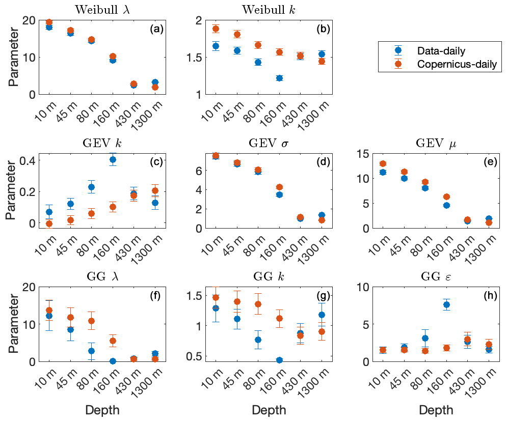
Figure 7 Same as Fig. 5 for the daily mean current speed of the data (blue circles) and 1 km resolution daily mean Copernicus model data.

We repeated the calculation of the Δ measure on the daily mean currents discussed above. The results are presented in the four bottom panels of Fig. 6. The conclusion with regards to the best pdf to model the current-speed time series remains unchanged although the actual Δ values are not the same. That is, also here, as for the conclusion based on the original data and 1 km resolution model, the central part of the distribution is best modeled by the GG pdf (for both the data and model), while for the tail of the distribution, for the measured currents, sometimes the GEV pdf is best fit to the data, whereas at other times, the GG pdf is the best fit to the data, and for the model, the GEV pdf is the best model.

Based on the above, the Copernicus 4.6 km resolution reanalysis better represents the statistical properties of the observed data in comparison to the 1 km resolution forward model of Solodoch et al. (2023). On the one hand, this is expected as the fundamental difference between these model types is that the reanalysis state is continuously “nudged” during its evolution to better agree with observational data. On the other hand, ideally, the higher-resolution model should provide a more accurate representation of the observations. However, the relevant bias of the 1 km model was in frequencies shorter than 10 inertial days, i.e., likely large-scale (mesoscale or basin-scale) currents, and their source may not necessarily be related to the fine resolution.

3.4 current-speed increment time series

Strong unusual currents like those of 2022 (Fig. 2) can affect the estimation of the fitted parameters. This is expressed by the different fitted parameters of the shorter observed current series presented in Fig. A4 (blue circles) in comparison to the entire series presented in Fig. 5. This suggests that longer current time series are needed for a more reliable estimation of the pdf parameters. Still, the temporal variations in the current speed are more stationary, and the study of their statistical properties may help to model ocean dynamics when including stochastic components. In other words, the equations of motion describe Newton's laws in terms of acceleration (the time derivative or the increments of the velocity). We thus study below the statistical properties of the current-speed increment time series.

We first present the distribution of the current-speed increment time series in Fig. 8 in both regular and semi-log plots. We used the normal (Eq. 5) and stretched exponential (Eq. 6) pdfs to fit the distribution of the data and found that the stretched exponential pdf better fit the data for both the central part of the distribution (left column of Fig. 8) and the tail of the distribution (right column of Fig. 8). It is evident that the tail of the distribution decays more slowly than the tail of the normal pdf (β=2) but faster than the exponential pdf (β=1). The exponent is between $\mathrm{1.1}\le \mathit{\beta }\le \mathrm{1.4}$, except for the deepest time series, for which the exponent is β=1.8. We observed similar behavior for the 1 km resolution current-speed increment time series (Fig. A9). Yet, it is clear the speed increments in the model are smaller than those of the data, especially for the deeper locations (Fig. A10).

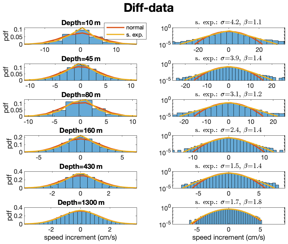
Figure 8 The pdfs of the current-speed increment time series in regular (left panels) and semi-log (right panels) plots. The corresponding depths are indicated in the title of the left panels, whereas the parameters of the fitted stretched exponential distribution are indicated in the title of the right panels. The fitted normal (red) and stretched exponential (yellow) are also included.

We summarize the estimated parameters of the stretched exponential and normal pdfs in Figs. A11 and A12, respectively. As expected, the scale parameter σ of the stretched exponential pdf decreases with depth (upper-left panel of Fig. A11) for both the data (blue) and model (red), although the model values are significantly lower than those of the data. This indicates that the model's variations are significantly smaller than those of the data; see also Fig. A10. The difference between the data and the model becomes smaller, yet significant when considering the time series that share the common times (lower-left panel of Fig. A11). The exponent β is larger for the data, indicating that the tail of the distribution decays faster for the measured data than the current-speed increment time series of the model (right panels of Fig. A11).

For β=2, the stretched exponential pdf takes the form of normal distribution; we present the estimated σ parameter (standard deviation) of the normal distribution in Fig. A12. We find that σ decreases with depth, as expected and similarly to the σ parameter of the stretched exponential pdf (Fig. A11). Also here, similarly to the stretched exponential pdf, the values of the data are larger than those of the 1 km resolution model parameter (right panel of Fig. A12). When considering the time series of the common times and the data and model, the parameter values of the data and the model are very similar.

Here we consider two pdfs to fit the current-speed increment time series and find that the stretched exponential pdf better fits the histograms than the normal pdf for both the data and model. Yet, even the stretched exponential pdf seems to underestimate the tail of the observed histograms (see the right-column panels of Figs. 8 and A9) such that other pdfs may better fit the current-speed increment time series.

4 Summary and discussions

We analyzed the probability distribution of the current-speed time series of the DeepLev station, which is located in the Levantine basin of the Mediterranean Sea, close to the coast of Israel. The current-speed time series span the depth of the water column from the surface to a depth of 1.3 km. We consider three pdfs that were previously used to model current and wind speed time series: the two-parameter Weibull pdf and the three-parameter GEV and GG pdfs. We find that the GG pdf best represents the current-speed time series across both the pdf central part and the tail.

We also analyzed a high-resolution regional model (Solodoch et al., 2023) and found that the GG pdf best fits the central part of the distribution of the simulated currents, while the tail of the distribution is better fitted by the GEV pdf. Additionally, the model's pdf are shifted to the right in comparison to the data's pdfs, indicating that the model exhibits stronger currents than the data (Fig. A3). Replacing the low-frequency amplitudes of the model's current time series with those of the data resulted in better correspondence to the observed current-speed distribution. Additionally, we examined the daily mean currents of the Copernicus reanalysis (Escudier et al., 2020) and found the statistics of these to be closer to the data than the 1 km resolution model. Still, as with the 1 km resolution model, the central part of the distribution for the Copernicus reanalysis is also best fitted by the GG pdf, while the GEV pdf better fits the tail.

The interannual variations in the current speed are relatively large such that a long time series is needed to more accurately estimate the parameters of the fitted pdf. In other words, the interannual variability of the fitted parameters may also be relatively large. Still, the variability in the current-speed time series is more stationary (not shown); we find that the distribution of the current-speed increment time series follows the stretched exponential pdf, with tails decaying faster than exponential but more slowly than Gaussian distribution. The current-speed increments of the data are larger than those of the model, especially in the deep ocean. A stretched exponential stochastic process together with temporal correlations of the current-speed time series may be used as a stochastic forcing in the equations of motion describing the internal dynamics of the ocean.

The climate in the eastern Mediterranean exhibits seasonal variability, with cold, rainy, and stormy winters and hot, dry, and relatively calm summers. Ocean currents also vary seasonally with relatively stronger currents during the winter. Thus, one would expect that the statistical properties are different during the winter and summer. Yet, since this seasonality is not strong and there are gaps in the data (Fig. 2), we did not perform a separate seasonal analysis and considered the entire time series as one process.

Finding the theoretical pdf that best models the current-speed data is important, e.g., for the estimation of the kinetic energy along the water column and for the estimation of power production. In addition, it may provide some knowledge regarding extreme current events. Yet, since the tail of the distribution is based on a few percent of the measurements, prediction of extreme events should be taken with caution and, if possible, used to estimate the uncertainty at the tails of the distribution.

The conclusion that the GG pdf is the best fit to the current-speed time series of the DeepLev station is based on the analysis of three pdfs: Weibull, GEV, and GG. It is possible that other pdfs may better fit the current-speed data. Yet, a better fit of four-parameter pdfs should be tested using the likelihood ratio test, if possible, to ensure that the better fit is not only due to the increased number of parameters. The same holds for the current-speed increment time series, for which we find the two-parameter stretched exponential pdf to be the best fit. Although the analysis and conclusions of this study are based on the specific location, the DeepLev mooring, we speculate that some of our conclusions (e.g., that the GG pdf is a good fit for the current-speed time series and that the current-speed increment time series follow the stretched exponential pdf) are valid for other locations around the world ocean (see, e.g,  Campisi-Pinto et al., 2020) and especially for the eastern Mediterranean.

Appendix A

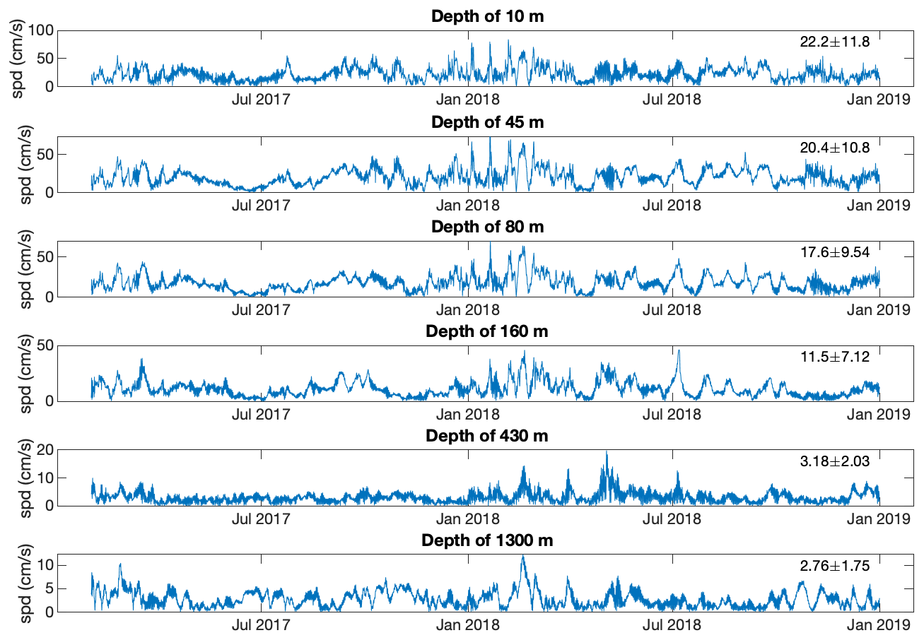
Figure A1 The model (1 km resolution) current-speed (in cm s⁻¹) time series for different depths. The numbers on the top right of each panel indicate the mean ± SD of the current time series.

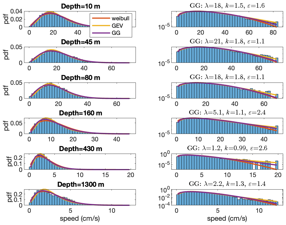
Figure A2 The pdfs of the (1 km resolution) model's current-speed time series shown in Fig. A1 in regular (left panels) and semi-log (right panels) plots. The corresponding depths are indicated in the title of the left panels, while the parameters of the fitted generalized gamma (GG) distribution are indicated in the title of the right panels. The fitted Weibull (red), GEV (yellow), and GG (purple) pdfs are also included.

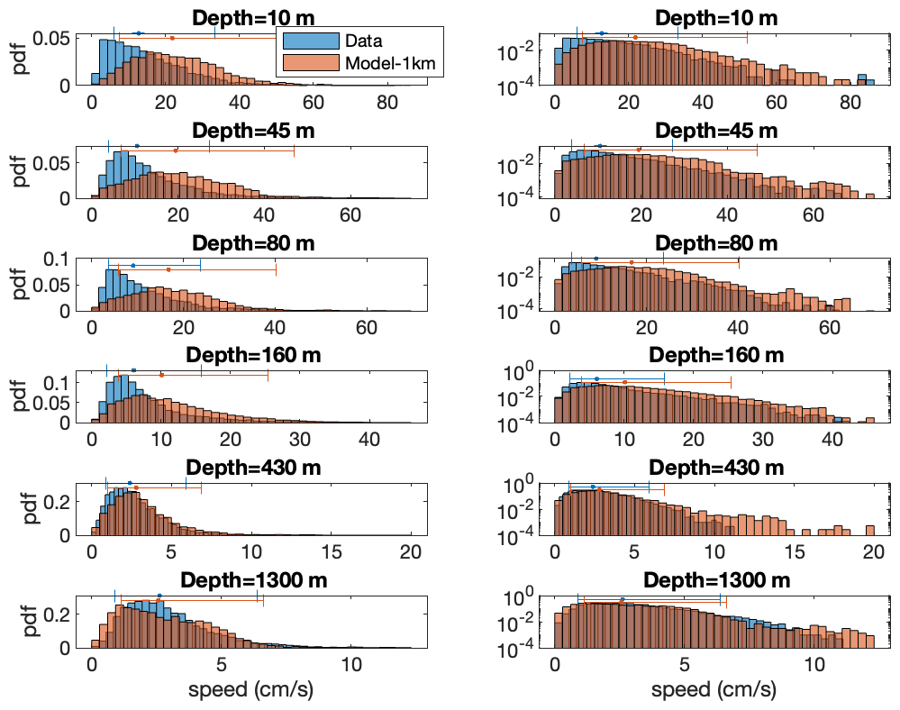
Figure A3 The data (blue) and model (light brown) pdfs of the current speed (2 h resolution) in regular (left panels) and semi-log (right panels) plots for time series of the common times of the data and model. The corresponding depths are indicated in the title of the panels. The overlapping part of the pdfs is indicated by the dark brown color, suggesting that model pdfs are stretched to the right for almost all depths.

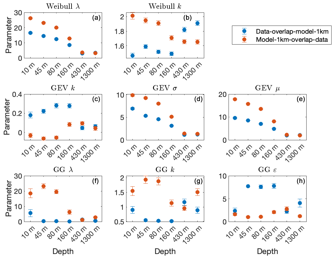
Figure A4 Same as Fig. 5 when using the data of the common times of the data and 1 km resolution model.

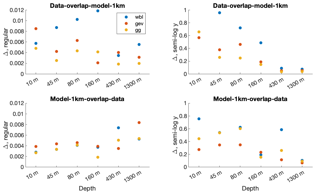
Figure A5 Same as the upper four panels of Fig. 6 for the data and model time series that share the same times.

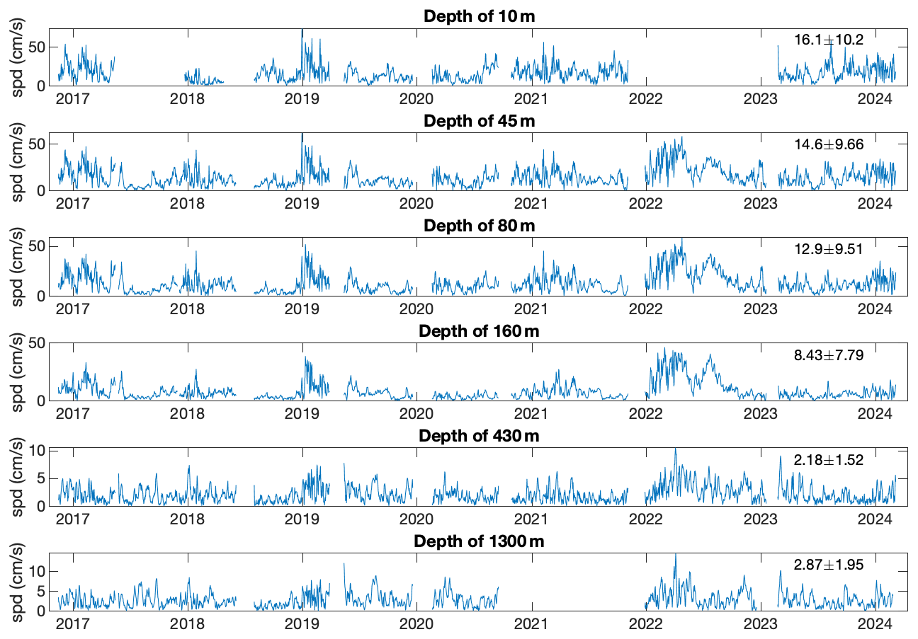
Figure A6 The observed data daily mean current-speed (in cm s⁻¹) time series for different depths. The numbers on the top right of each panel indicate the mean ± SD of the current time series.

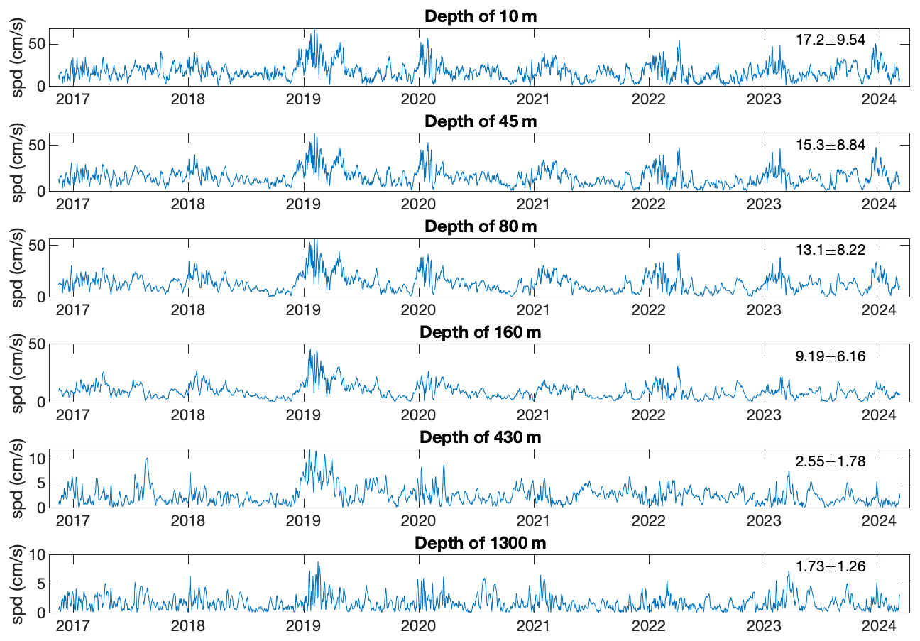
Figure A7 The Copernicus reanalysis daily mean current-speed (in cm s⁻¹) time series (Escudier et al., 2020) for different depths. The numbers on the top right of each panel indicate the mean ± SD of the current time series.

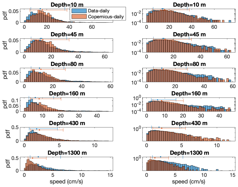
Figure A8 The data (blue) and Copernicus reanalysis (light brown) pdfs of the current speed (daily mean) in regular (left panels) and semi-log (right panels) plots. The corresponding depths are indicated in the title of the panels. The overlapping part of the pdfs is indicated by the dark brown color. The blue and light brown error bars indicate the median and 25 %–75 % quantiles.

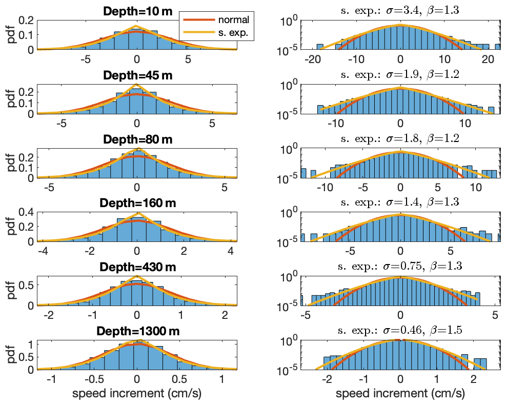
Figure A9 The pdfs of the (1 km resolution) model's current-speed increment time series in regular (left panels) and semi-log (right panels) plots. The corresponding depths are indicated in the title of the left panels, while the parameters of the stretched exponential distribution are indicated in the title of the right panels. The fitted normal (red) and stretched exponential (yellow) pdfs are also included. Note the smaller horizontal range of the distribution in comparison to those of the measured data (Fig. 8).

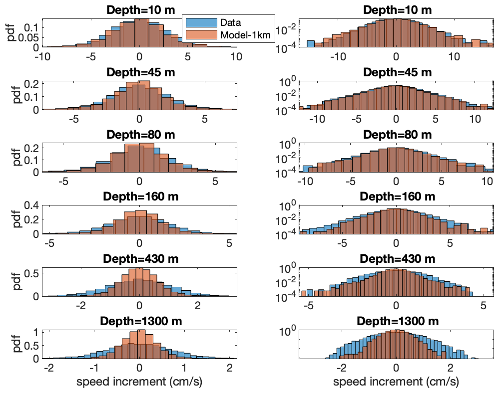
Figure A10 The data (blue) and model (light brown) pdfs of the current-speed increments (2 h resolution) in regular (left panels) and semi-log (right panels) plots for time series of the common times of the data and model. The corresponding depths are indicated in the title of the panels. The overlapping part of the pdfs is indicated by the dark brown color. Note that the tails of the data's pdfs span further than that of the model, indicating that the speed increments of the data are larger than those of the model.

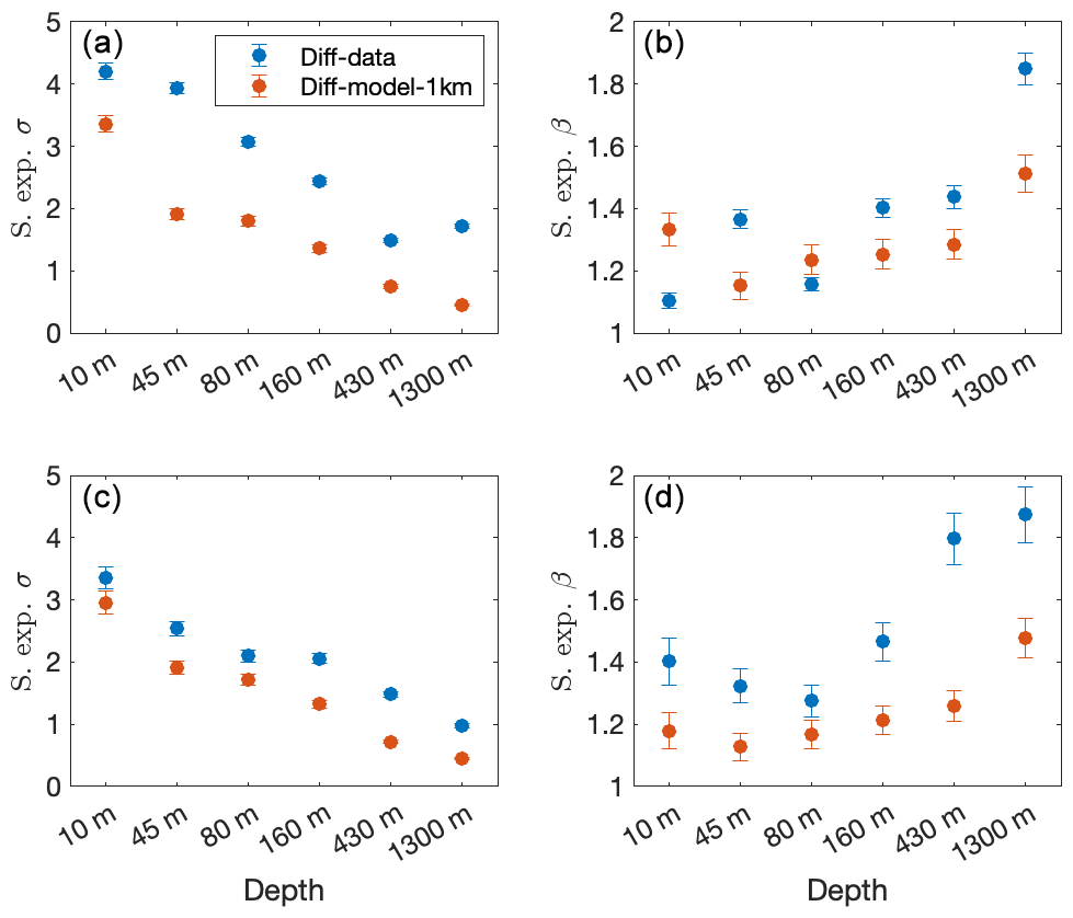
Figure A11 The estimated parameters σ (right panels) and β (left panels) of the stretched exponential pdf versus the depth of the current-speed increment of the data (blue circles) and 1 km resolution model (red circles). The upper panels depict the results of the original data and 1 km resolution model currents, while the lower panels depict the results of time series for the common measurement times (intersection). The error bars indicate the 5 %–95 % confidence interval (which is not always visible).

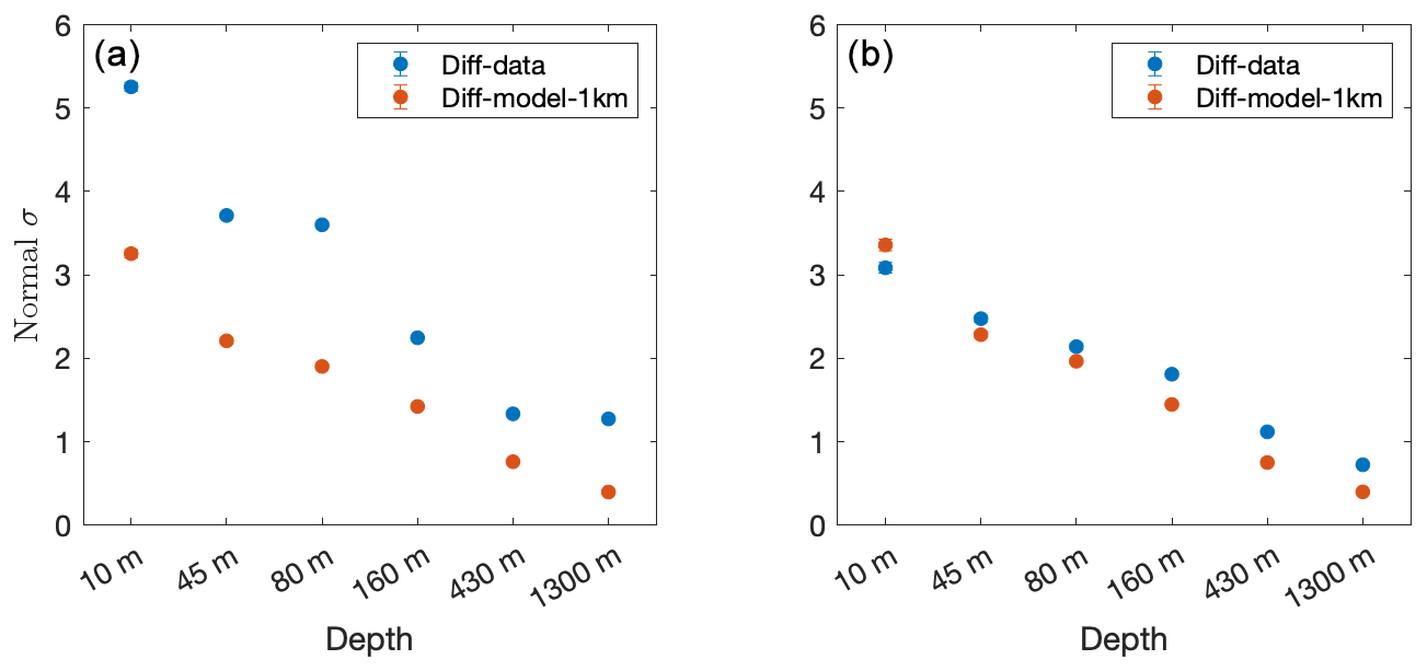
Figure A12 The estimated parameter σ of the normal pdf versus the depth of the current-speed increment of the data (blue circles) and 1 km resolution model (red circles). The left panel depicts the results of the original data and 1 km resolution model currents, while the right panel depicts the results of the time series for the common measurement times (intersection). The error bars indicate the 5 %–95 % confidence interval (which are too small to be visible).

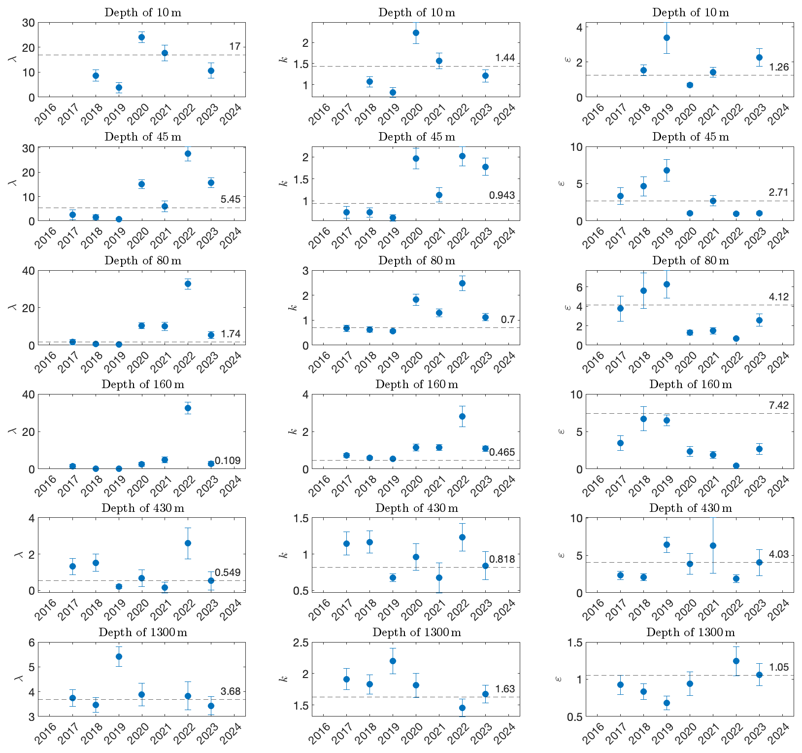
Figure A13 The annual estimated GG distribution parameters that are based on the measured current-speed time series shown in Fig. 2. We show the parameters only when the number of data points spans more than half a year. The horizontal dashed lines represent the estimated parameter of the entire time series. Note that the estimated GG parameters for depths of 80 and 160 m (third and fourth rows) are inaccurate as the MLE did not converge. The error bars indicate the 5 %–95 % confidence interval.