Turbulent dissipation along contrasting internal tide paths off the Amazon shelf from AMAZOMIX

The Amazon shelf break is a key oceanic region where strong internal tides (ITs) are generated, playing a substantial role in climate processes and ecosystems through vertical dissipation and mixing. During the AMAZOMIX survey (2021), currents, hydrography, and turbulence were measured over the M₂ tidal period (12.42 h) at multiple stations along both high (HTE) and low (LTE) tidal energy paths, covering IT generation and propagation regions off the Amazon shelf. This dataset provides a unique opportunity to assess IT-driven vertical dissipation and quantify its spatial extent and influence in the region.

Microstructure analyses, integrated with hydrographic data, highlighted contrasting dissipation rates. The highest rates occurred at IT generation sites along the HTE paths, while the lowest rates were observed on the slope along the LTE path. Near generation sites, the dissipation rates were elevated, [10⁻⁶] W kg⁻¹, with IT shear contributing ∼60 % compared to the mean baroclinic current (MBC) shear. Along IT paths, rates decreased to [10⁻⁸] W kg⁻¹ but remained substantial, driven by nearly equal contributions from IT and MBC shear.

A key finding was the relative increase in turbulent dissipation ([10⁻⁷] W kg⁻¹) ∼230 km from two distinct IT generation sites at the shelf break. This zone of high mixing was located in an area where the general circulation vanished, coinciding with a region of potential constructive interference of IT rays originating from different generation sites. It also aligned with the occurrence of large-amplitude internal solitary waves (ISWs), suggesting that constructive IT ray interference may generate nonlinear ISWs that lead to enhanced dissipation.

1 Introduction

Turbulent mixing in the ocean is essential for sustaining thermohaline and meridional overturning circulation and for maintaining the global ocean energy budget (Koch-Larrouy et al., 2010; Kunze, 2017). It regulates climate by controlling heat and carbon transport and providing nutrients for photosynthesis (Huthnance, 1995; Munk and Wunsch, 1998). Mixing effects are often reflected in step-like density features, indicating homogeneous regions (Koch-Larrouy et al., 2015; Bouruet-Aubertot et al., 2018). Ocean mixing can be driven by processes like current shear (Miles, 1961; Rainville and Pinkel, 2006; Whalen et al., 2012), river plumes (Ruault et al., 2020), fronts (Geyer, 1995), overturns (Munk and Wunsch, 1998; Thorpe, 2018), and tides (Zhao et al., 2012).

Barotropic tides interacting with sharp topography generate internal tides (ITs), strong internal waves at tidal frequencies and harmonics (Zhao et al., 2016). ITs can create strong vertical displacements of up to tens of meters (Garrett and Kunze, 2007) and may propagate offshore. As they propagate, ITs can interact with topography, stratification, waves, currents, and eddies (Whalen et al., 2012; Bordois, 2015; Ivey et al., 2020; Inall et al., 2021), leading to complex offshore mixing (Gill, 2012). ITs can also destabilize, break, and dissipate locally (Zhao et al., 2016), and their intensity and path can change due to environmental factors, potentially generating nonlinear internal solitary waves (ISWs; Jackson et al., 2012).

These processes are prominent in the Amazon River–ocean continuum (AROC) in the western tropical Atlantic. This dynamic region, shaped by interactions between currents, eddies, the Amazon River plume, and internal waves, drives complex circulation and vertical mixing. The North Brazil Current (NBC), the region's dominant western boundary current, flows northwest along the coast (Fig. 1), with velocities of ∼1.2 m s⁻¹ and a vertical extent of up to 100 m, transporting warm, saline waters from the South Atlantic (Barnier et al., 2001). The NBC influences the Amazon plume's dispersal and contributes to mesoscale eddy formation (Johns et al., 1998; Bourlès et al., 1999; Neto and Silva, 2014). The Amazon plume shows strong seasonal variability, extending up to 1500 km offshore during the rainy season (May–July) and retreating to under 500 km during the dry season (September–November; Coles et al., 2013).

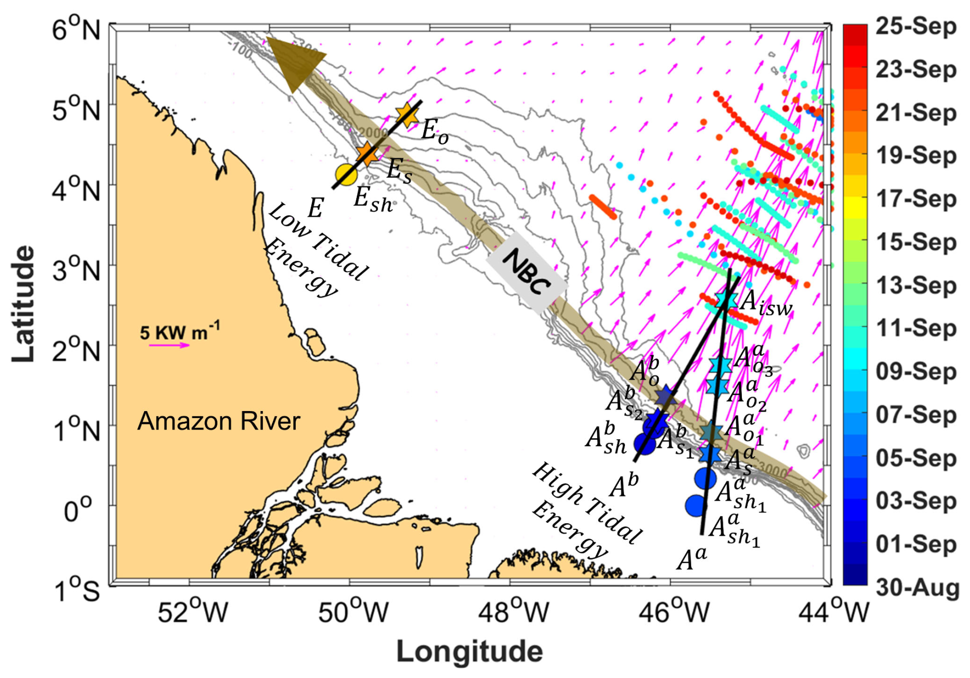
Figure 1 Map of a part of the AMAZOMIX 2021 cruise off the Amazon shelf showing bathymetric contours (100, 750, 2000, and 3000 m isobaths) in grey. Magenta arrows show the 25 h mean depth-integrated baroclinic IT energy flux (September 2015, from the NEMO model) originating from IT generation sites (A^a, A^b, and E) along the shelf break. Solid black lines depict transects (A^a, A^b, and E) defined on the high tidal energy (HTE) and low tidal energy (LTE) paths. The solid brown line represents the NBC pathways, illustrating background circulation. Shattered colored lines highlight ISW signatures. Colored circles and stars indicate short and long CTD-O₂/L-S-ADCP stations, respectively, with the corresponding sampling dates represented by the color bar. The superscripts “a” and “b” on station names correspond to sites A^a and A^b, respectively. The subscripts “sh”, “s”, “o”, and “isw” indicate station locations: shelf ($A_{{\text{sh}}_{\mathrm{1}}}^a$, $A_{{\text{sh}}_{\mathrm{2}}}^a$, $A_{\text{sh}}^b$, and E_sh), slope ($A_{\mathrm{s}}^a$, $A_{{\mathrm{s}}_{\mathrm{1}}}^b$, $A_{{\mathrm{s}}_{\mathrm{2}}}^b$, and E_s), open ocean ($A_{{\mathrm{o}}_{\mathrm{1}}}^a$, $A_{{\mathrm{o}}_{\mathrm{2}}}^a$, $A_{{\mathrm{o}}_{\mathrm{3}}}^a$, $A_{\mathrm{o}}^b$, and E_o), and ISW regions (A_isw) for sites A^a, A^b and E, respectively.

At the Amazon shelf break, internal waves, such as ITs and ISWs, are generated, propagate, and dissipate. These waves have been observed through in situ measurements (Brandt et al., 2002) and synthetic-aperture radar (SAR) satellite imagery (Magalhães et al., 2016). Recently, de Macedo et al. (2023) used MODIS images to identify frequent mode-1 ISWs originating from two IT generation sites (A^a and A^b; Figs. 1 and 2a, b), with wavelengths ranging from 72 to 128 km. These ISWs appeared where Tchilibou et al. (2022) predicted IT energy dissipation using numerical modeling. Their findings suggest that ∼30 % of M₂ IT energy dissipates near the generation sites on the slope (A^a, A^b, and E; Fig. 1), corresponding to higher-mode ITs, while lower-mode ITs propagate offshore, where they dissipate and enhance mixing. Offshore mixing may result from shear instabilities driven by interactions between the currents, eddies, Amazon plume, ITs, and coupled processes (e.g., wave–wave, wave–current, or plume–wave interactions). However, no direct dissipation measurements have been made in this region to quantify IT-driven mixing.

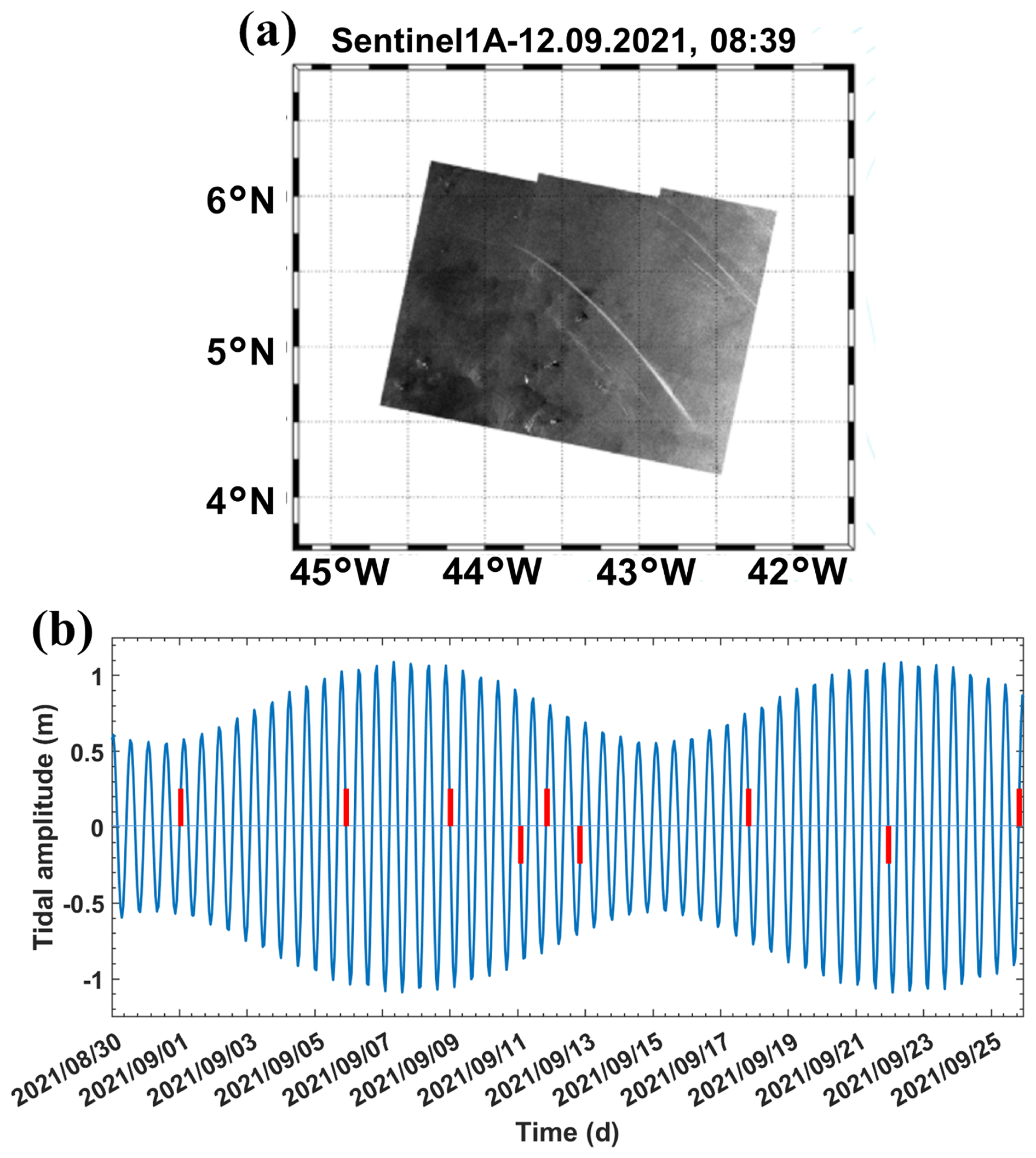
Figure 2 (a) 1A Sentinel image acquired on 12 September 2021 showing ISW signatures. (b) Tidal (M₂ and S₂) amplitude of the currents (at 1° N, −45.5° W) derived from the FES2014 model (Lyard et al., 2021). ISW signature dates are marked by red bars.

To address this, the AMAZOMIX cruise (Bertrand et al., 2021) was conducted to investigate IT-driven mixing off the Amazon shelf. Microstructure and hydrographic measurements were collected at repeated stations over an M₂ tidal cycle (∼12.42 h), providing dissipation estimates and insights into associated processes. Stations were positioned along contrasting IT paths, such as high tidal energy (HTE) paths (sites A^a and A^b; Fig. 1) and low tidal energy (LTE) path (site E; Fig. 1), enabling dissipation quantification in varying tidal regimes. The AMAZOMIX dataset provides a unique opportunity to assess the role of ITs in mixing within the AROC region.

2 Data and methods

2.1 Data collection

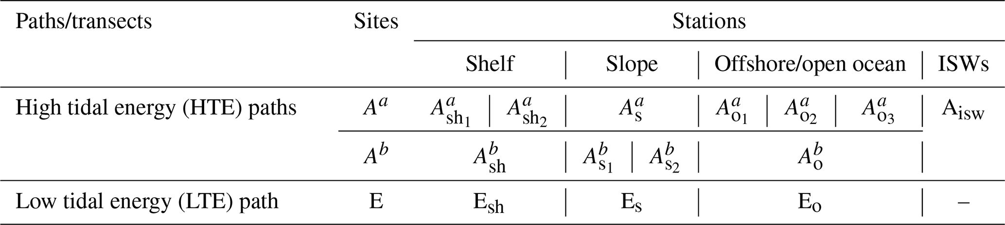
The AMAZOMIX cruise (Bertrand et al., 2021) was performed over the shelf/slope areas off the AROC during August–October 2021 aboard the IRD vessel RV Antea. At each designated site, 12 h stations were set up with repeated casts (four–five casts per site) of Conductivity–Temperature–Depth–Oxygen (CTD-O₂)/Lowered Acoustic Doppler Current Profiler (LADCP) and Velocity Microstructure Profiler (VMP) to measure the turbulent kinetic energy (TKE) dissipation rates over a complete tidal (M₂) cycle, allowing for the separation of the tidal component from the total current. A high-resolution ($\mathrm{1}/\mathrm{36}$°) NEMO (Nucleus for European Modeling of the Ocean) model (Madec et al., 2019) was used to determine station locations based on realistic IT generation and propagation maps (Tchilibou et al., 2022; Assene et al., 2024) and to estimate the mean background stratification. Measurement stations for short- and long-duration (∼12 h) deployments were systematically named and organized by location along the HTE and LTE paths. Stations at sites A^a and A^b were marked with superscripts “a” and “b”, respectively. Subscripts denoted specific regions: “sh” for shelf ($A_{{\text{sh}}_{\mathrm{1}}}^a$, $A_{{\text{sh}}_{\mathrm{2}}}^a$, $A_{\text{sh}}^b$, and E_sh), “s” for slope ($A_{\mathrm{s}}^a$, $A_{{\mathrm{s}}_{\mathrm{1}}}^b$, $A_{{\mathrm{s}}_{\mathrm{2}}}^b$, and E_s), “o” for offshore/open ocean ($A_{{\mathrm{o}}_{\mathrm{1}}}^a$, $A_{{\mathrm{o}}_{\mathrm{2}}}^a$, $A_{{\mathrm{o}}_{\mathrm{3}}}^a$, $A_{\mathrm{o}}^b$, and E_o), and “isw” for ISW regions (A_isw) (Fig. 1, Table A1, Appendix A).

CTD-O₂ measurements were obtained using a Seabird 911 Plus with dual sensors mounted in the rosette. The 24 Hz CTD-O₂ sensors were calibrated before and after the cruise to ensure accurate dissolved oxygen measurements throughout the survey. The temperature, salinity, and oxygen standard deviation between the CTD-O₂ sensors and the bottle samples was 0.003 °C, 0.003 PSU, and 0.05 mL L⁻¹, respectively. CTD-O₂ data were averaged over 1 m bins to filter out spikes and missing points and aligned in time to correct the lag effects.

Two 300 kHz RDI LADCPs were mounted on the rosette to provide vertical current profiles with 8 m resolution supplemented by 75 kHz shipboard ADCP (SADCP) profiles recorded continuously during the cruise. Vertical resolution of SADCP was adjusted according to bottom depth, e.g., 8 m for depths >150 m (at $A_{{\mathrm{s}}_{\mathrm{2}}}^b$, $A_{\mathrm{o}}^b$, $A_{\mathrm{s}}^a$, A_isw, E_s, and E_o) and 4 m for other depths. Data processing and quality control followed GO-SHIP Repeat Hydrography Manual protocols. In total, 71 CTD-O₂/LADCP profiles were collected during the AMAZOMIX cruise.

To characterize mixing, the TKE microstructure profiles were obtained from high-frequency (∼2 mm resolution) measurements of temperature and velocity shear using a VMP-250 profiler (Rockland Scientific International, Inc.) capable of reaching depths up to 1000 m. The VMP-250 features two high-resolution thermistors (FP07) and two high-resolution velocity shear probes (probes 1 and 2; with 5 % signal accuracy) with a sampling rate of 1024 Hz. The profiler was deployed and retrieved via an electric winch and rope tether with alternating deployments between the CTD-O₂/LADCP profiles at 33 stations, yielding a total of 201 profiles. For this study, data from 14 stations comprising SADCP data, 109 VMP profiles, and 54 CTD-O₂/LADCP profiles are analyzed.

2.2 Methods

2.2.1 TKE dissipation rates

The VMP data are processed using the ODAS MATLAB library (developed by Rockland Scientific International, Inc.) to infer the TKE dissipation rate (ε). The processing methods for the VMP data are briefly described here and adhere to the recommendations of ATOMIX (Analyzing ocean Turbulence Observations to quantify MIXing), as reported by Lueck et al. (2024), and have been validated against the benchmark estimates (presented in Fer et al., 2024).

First, the VMP data are converted into physical shear units, and the time series are prepared. Continuous sections of the time series are selected for dissipation estimation. Before spectral estimation, the aberrant shear signals caused by vessel wake contamination are removed. Collisions of the shear probe with plankton and other particles are removed using the de-spiking routine. The records from each section are then high-pass-filtered (e.g., at station $A_{{\mathrm{s}}_{\mathrm{2}}}^b$; Fig. 3).

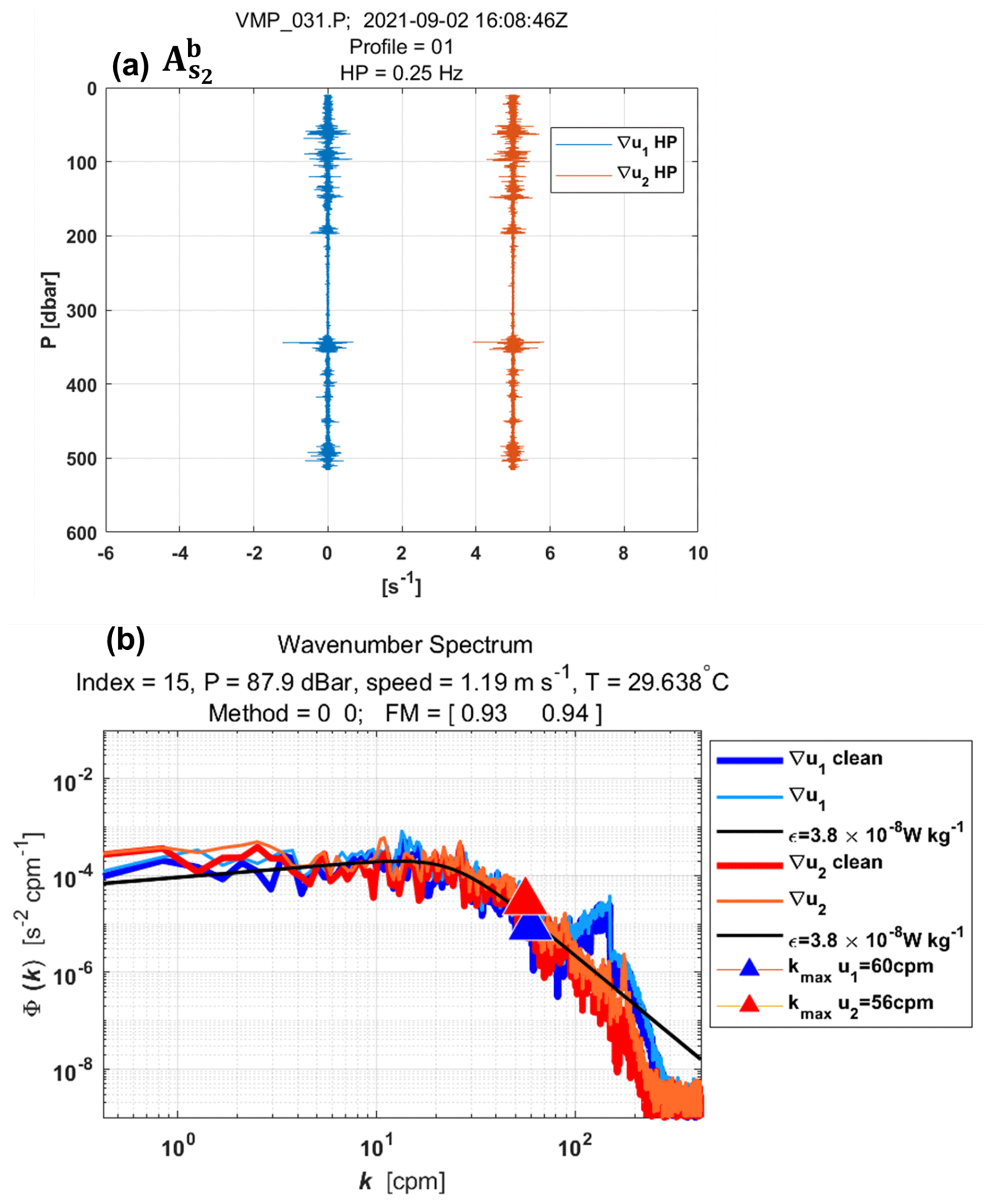
Figure 3 Example of wavenumber spectra from a dissipation structure segment used to determine the dissipation rate at station $A_{{\mathrm{s}}_{\mathrm{2}}}^b$ at a pressure of 87.9 dbar. (a) Cleaned and high-pass filtered signals from shear probe 1 (blue) and shear probe 2 (red, offset by 5 s⁻¹). (b) Wavenumber spectra for shear probes 1 and 2. Thick lines (blue for probe 1, red for probe 2) show shear spectra with coherent noise correction, while thin lines (sky blue for probe 1, orange for probe 2) show spectra without correction. Triangles mark the maximum wavenumber used for dissipation rate estimation. Black lines represent Nasmyth reference spectra for an estimated dissipation rate of $\mathrm{3.8}\times {\mathrm{10}}^{-\mathrm{8}}$ W kg⁻¹ for both shear probes. Dissipation rate estimates for shear probe 1 and shear probe 2 at a pressure of 87.9 dbar yielded a figure of merit of 0.93 and 0.94, respectively.

Shear spectra are estimated using record lengths (L) and fast Fourier transform segments of 2 s, which are cosine-windowed and overlapped by 50 % (e.g., at station $A_{{\mathrm{s}}_{\mathrm{2}}}^b$; Fig. 3). Additionally, vibration-coherent noise is removed. Different L and overlap (O) settings were selected and tested based on the environment (e.g., deep vs. shallow water) following Fer et al. (2024). For shallow stations, L (O) was shortened to 5 s (2.5 s), in contrast to the 8 s (4 s) used for deeper stations, due to evidence of overturns observed in AMAZOMIX acoustic measurements at deeper stations (Ariane Koch-Larrouy, personal communication, 20 September 2024). This adjustment helped to optimize the spatial resolution of dissipation estimates in shallow water stations.

Finally, ε is determined using the spectral integration method and by comparison with the Nasmyth empirical spectrum (Nasmyth, 1970). Quality assurance tests are carried out in accordance with ATOMIX's recommendations (Lueck et al., 2024). A figure of merit <1.4 is used to exclude bad data (e.g., at station $A_{{\mathrm{s}}_{\mathrm{2}}}^b$; Fig. 3), and the fraction of data affected by de-spiking is <0.05.

Subsurface mixing, driven by IT breaking and shear instabilities, substantially influences the base of the mixed layer, particularly in equatorial waters (Gregg et al., 2003). To analyze midwater dissipation rates (excluding surface and bottom boundary layers), we define the following depths: mixed layer depth (MLD), mixing layer depth (XLD), and bottom boundary layer (BBL) thickness (H_BBL).

There are several criteria for defining the MLD. In this study, we use the commonly accepted density threshold criterion of 0.03 kg m⁻³, as defined by de Boyer Montégut et al. (2004) and Sutherland et al. (2014), to estimate the MLD (Table B1, Appendix B).

The XLD is defined as the depth at which ε decreases to a background level (Sutherland et al., 2014). Previous studies have applied various thresholds for background dissipation levels, such as 10⁻⁸ and 10⁻⁹ W kg⁻¹ in higher latitudes based on in situ observations (Brainerd and Gregg, 1995; Lozovatsky et al., 2006; Cisewski et al., 2008; Sutherland et al., 2014) and 10⁻⁵ m² s⁻¹ using an ocean general circulation model (Noh and Lee, 2008). In this study, the XLD is specified as the depth where ε decreases from the first minimum value (e.g., 10⁻⁹ W kg⁻¹ for $A_{\mathrm{o}}^b$) (Table B1, Appendix B). This aligns with previous dissipation thresholds and ensures that dissipation is captured in midwater. Huang et al. (2019) showed that the H_BBL spatially varies between 15 and 123 m in the Atlantic Ocean, with a median of ∼30–40 m in the North Atlantic. According to their findings, and based on bathymetry measurements and near-bottom current measurements from CTD-O₂/LADCP, we define the H_BBL in our study as 18 m for shallow stations and 40 m for deep stations.

2.2.2 Baroclinic currents

To analyze the processes explaining dissipation and mixing, particularly along IT paths, we estimate shear instabilities associated with the semi-diurnal (M₂) ITs and mean circulation as well as their contributions to mixing.

The M₂ tidal component of the tidal current is derived by calculating the baroclinic (semi-diurnal) tidal velocity $[u^{\prime \prime },v^{\prime \prime }]$ following these equations:

$$\begin{array}{}\text{(1)}& {\displaystyle }[u^{\prime },v^{\prime }]=[u,v]-[u_{\text{bt}},v_{\text{bt}}],\text{(2)}& {\displaystyle }[u_{\text{bt}},v_{\text{bt}}]={\displaystyle \frac{\mathrm{1}}{H}}{\int }_{-H}^{\mathrm{0}}[u,v]\mathrm{d}z,\text{(3)}& {\displaystyle }[u^{\prime \prime },v^{\prime \prime }]=[u^{\prime },v^{\prime }]-[\stackrel{\mathrm{‾}}{u^{\prime }},\stackrel{\mathrm{‾}}{v^{\prime }}].\end{array}$$

Here, [u,v] represent total horizontal (zonal u and meridional v) velocities obtained from SADCP data. The components $[u^{\prime },v^{\prime }]$ and [u_bt,v_bt] represent baroclinic and barotropic components of horizontal velocities, respectively. H is water depth. The baroclinic mean velocities $[\stackrel{\mathrm{‾}}{u^{\prime }},\stackrel{\mathrm{‾}}{v^{\prime }}]$, calculated to estimate mean circulation along IT paths, are decomposed into along-shore $\stackrel{\mathrm{‾}}{{u^{\prime }}_{\mathrm{l}}}$ and cross-shore $\stackrel{\mathrm{‾}}{{u^{\prime }}_{\mathrm{c}}}$ velocities. The overbar denotes the average over the M₂ tidal period. Similarly, the components $[u^{\prime \prime },v^{\prime \prime }]$ are decomposed into along-shelf ${u^{\prime \prime }}_{\mathrm{l}}$ and cross-shelf ${u^{\prime \prime }}_{\mathrm{c}}$ velocities. The along-shelf velocity component is defined parallel to the 200 m isobath (treated as the coastline), with positive values indicating northwestward flow and negative values indicating southeastward flow. The cross-shelf velocity component is defined perpendicular to the 200 m isobath, with positive values indicating northeastward flow and negative values indicating southwestward flow.

Note that continuously collected SADCP for some stations are not sufficiently resolved due to gaps filled by interpolating between time points. The similar processing is applied to the CTD-O₂ data. SADCP time series data are less than 17 h at all long stations, except for S14, which spans 42 h. As a result, the diurnal and semi-diurnal period fittings are not formally distinct (except at A_isw), and the inertial period (at least 5 d) cannot be resolved in our dataset. This limits our ability to separate currents by frequency and examine the associated dissipation. The velocity profiles from LADCP are glued into our SADCP time series data below ∼500 m depth at long stations.

To evaluate shear instabilities associated with ITs and the mean background circulation, we compute the baroclinic tidal vertical shear squared ($S^{{\mathrm{2}}^{\prime \prime }}$) and mean shear squared ($\stackrel{\mathrm{‾}}{S^{{\mathrm{2}}^{\prime }}}$) as follows:

$$\begin{array}{}\text{(4)}& {\displaystyle }{S}^{{\mathrm{2}}^{\prime \prime }}=(\partial u^{\prime \prime }/\partial z{)}^{\mathrm{2}}+(\partial v^{\prime \prime }/\partial z{)}^{\mathrm{2}},\text{(5)}& {\displaystyle }\stackrel{\mathrm{‾}}{S^{{\mathrm{2}}^{\prime }}}=(\partial \stackrel{\mathrm{‾}}{u^{\prime }}/\partial z{)}^{\mathrm{2}}+(\partial \stackrel{\mathrm{‾}}{v^{\prime }}/\partial z{)}^{\mathrm{2}}.\end{array}$$

The individual contributions of semi-diurnal ITs and mean circulation are then expressed as follows: $S^{{\mathrm{2}}^{\prime \prime }}/(\stackrel{\mathrm{‾}}{S^{{\mathrm{2}}^{\prime }}}+S^{{\mathrm{2}}^{\prime \prime }})$ for IT contribution and $\stackrel{\mathrm{‾}}{S^{{\mathrm{2}}^{\prime }}}/(\stackrel{\mathrm{‾}}{S^{{\mathrm{2}}^{\prime }}}+S^{{\mathrm{2}}^{\prime \prime }})$ for mean circulation contribution. This calculation is used to quantify the contribution of tidal or mean shear during each dissipation event.

2.2.3 Ray-tracing calculation

Analyzing both the mean currents and the spatial dimension along the IT pathways offers another insight into the mechanisms responsible for observed mixing (Rainville and Pinkel, 2006). IT energy rays are generated in regions with steep topography, such as the shelf break, where the IT slope matches the bottom slope (i.e., critical slopes) before propagating within the ocean interior. These rays, moving both downward and upward, encounter the seasonal pycnocline, resulting in beam scattering and the formation of large IT oscillations. As these oscillations steepen, they disintegrate into nonlinear ISWs, a process known as “local generation” of ISWs (New and Pingree, 1992). To explore IT paths, ray-tracing techniques are employed, as previously used by New and da Silva (2002) and Muacho et al. (2014), to investigate the effectiveness and expected pathways of the IT beams off the Amazon shelf. One main assumption in our linear-theory-based hypothesis is that stratification remains horizontally uniform along the IT propagation path, although in reality, it may vary due to submesoscale and mesoscale variability. This limitation makes the ray tracing approach less realistic but still useful as a first-order estimate of energy distribution. The IT ray-tracing calculation assumes that in a continuously stratified fluid, IT's energy can be described by characteristic pathways of beams (or rays) with a slope c to the horizontal:

$$\begin{array}{}\text{(6)}& c=\pm {\left({\displaystyle \frac{{\mathit{\sigma }}^{\mathrm{2}}-f^{\mathrm{2}}}{N^{\mathrm{2}}-{\mathit{\sigma }}^{\mathrm{2}}}}\right)}^{\mathrm{1}/\mathrm{2}},\end{array}$$

where σ is the M₂ tidal frequency ($\mathrm{1.4052}\times {\mathrm{10}}^{-\mathrm{4}}$ rad s⁻¹) and f is the Coriolis parameter. Here, N² is the buoyancy frequency squared, which is calculated using the sorted potential density profiles (σ_θ). It is given by $N^{\mathrm{2}}=-(g/{\mathit{\rho }}_{\mathrm{0}})(\mathrm{d}{\mathit{\sigma }}_{\mathit{\theta }}/\mathrm{d}z)$, where ρ₀ is a reference density (1025 kg m⁻³) and g is the gravitational acceleration. N² is obtained from time-averaged AMAZOMIX CTD-O₂ data glued with monthly N² profiles from Amazon36 (NEMO model outputs, 2012–2016) below 1000 m depth. Amazon36 is a specific configuration specifically designed to cover the western tropical Atlantic from the mouth of the Amazon River to the open sea (see Tchilibou et al., 2022, and Assene et al., 2024, for configuration details and model description). The NEMO model's fine horizontal resolution ($\mathrm{1}/\mathrm{36}$°) and 75 vertical levels allow for accurate simulation of low-mode ITs generated along the Brazilian shelf break. Key inputs include bathymetric data from the 2020 General Bathymetric Chart of the Oceans, surface forcing from ERA-5 atmospheric reanalysis (Hersbach et al., 2020), and river runoff data from the ISBA (Interaction Sol-Biosphère-Atmosphère; https://www.umr-cnrm.fr/spip.php?article146&lang=en, last access: 20 September 2024) model. Open boundary conditions were driven by 15 major tidal constituents (M₂, S₂, N₂, K₂, 2N₂, MU₂, NU₂, L₂, T₂, K₁, O₁, Q₁, P₁, S₁, and M₄) and barotropic currents from the FES2014 atlas (Lyard et al., 2021) supplemented by temperature, salinity, and velocity data from the MERCATOR-GLORYS12v1 assimilation product (Lellouche et al., 2018).

Using N² profiles from both AMAZOMIX and Amazon36, IT ray-tracing diagrams are performed along the transects. The upper (UTD) and lower (LTD/LPD) thermocline/pycnocline depth are delimited as defined by Assunçao et al. (2020). UTD corresponded to the depth where the vertical temperature gradient $\partial \mathit{\theta }/\partial z=\mathrm{0.1}$ °C m⁻¹, while LTD/LPD were the last depths below the UTD at which $N^{\mathrm{2}}\ge {\mathrm{10}}^{-\mathrm{4}}$ s⁻². Seasonal sensitivity tests of rays (August, September, October, and April) are conducted by varying the critical slope positions and N² to explore its influence and generate a set of ray paths consistent with characteristics of IT paths.

3 Results

3.1 Mixing

3.1.1 Thermohaline and IT features

In this subsection, we analyze density profiles (up-cast and down-cast) taken approximately 6 h apart (half the M₂ tidal period) along three transects (A^a, A^b, and E) defined on the HTE and LTE paths. Our aim is to examine the effects of mixing on water mass and the signatures of wave propagation.

First, mixing effects are evidenced in the step-like features of the density profiles (Fig. 4), indicating homogeneous layers. The vertical extent of these layers ($L_{{\mathit{\rho }}_{\mathrm{c}}}$; Fig. 4b) is determined, where the density gradient falls below the homogeneous threshold (0.01 kg m⁻³) between 60 and 180 m depth, ranging from 4 to 41 m. These step-like features are more pronounced along the HTE transects (A^a and A^b), with examples including 10 m at $A_{\mathrm{s}}^a$, 41 m at $A_{{\mathrm{o}}_{\mathrm{2}}}^a$, 13 m at $A_{{\mathrm{o}}_{\mathrm{3}}}^a$, and 20 m at A_isw compared to the LTE transect E, where they are smaller (e.g., 4 m at E_s).

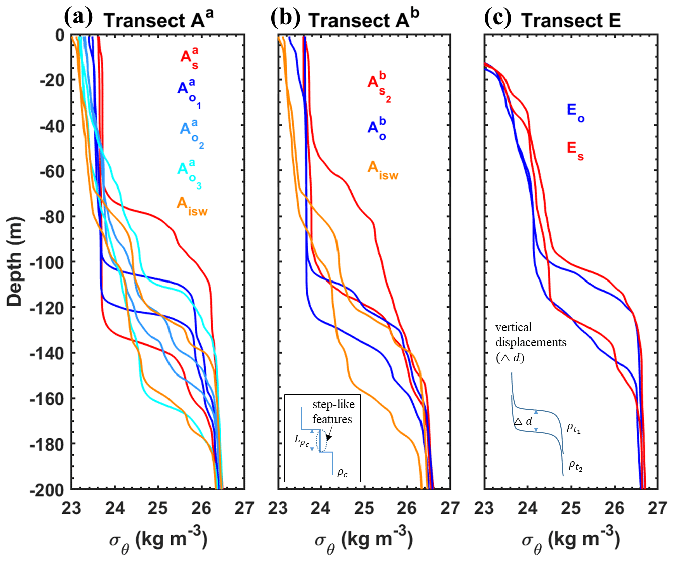
Figure 4 Density profiles (σ_θ, kg m⁻³) from CTD-O₂ measurements during the AMAZOMIX 2021 cruise along transects (a) A^a, (b) A^b, and (c) E. For long stations ($A_{{\mathrm{s}}_{\mathrm{2}}}^b$, $A_{\mathrm{o}}^b$, $A_{\mathrm{s}}^a$, $A_{{\mathrm{o}}_{\mathrm{1}}}^a$, $A_{{\mathrm{o}}_{\mathrm{2}}}^a$, $A_{{\mathrm{o}}_{\mathrm{3}}}^a$, A_isw, E_s, and E_o), two density profiles recorded ∼6 h apart (half the M₂ tidal period) are shown to highlight step-like structures and vertical isopycnal displacements along the transects. Colored lines represent stations on the slope (red) and open ocean (blue, sky blue, cyan, and light orange). The subpanel in panel (b) depicts a step-like structure, where $L_{{\mathit{\rho }}_{\mathrm{c}}}$ represents the vertical extent of homogeneous regions and ρ_c denotes the density structure. The subpanel in panel (c) illustrates vertical displacements (Δd) of density structures, with ${\mathit{\rho }}_{t_{\mathrm{1}}}$ and ${\mathit{\rho }}_{t_{\mathrm{2}}}$ representing density structures at times t₁ and t₂, respectively.

Second, wave propagation signatures are inferred from vertical displacements of isopycnals (constant density surfaces) between the two sampling times (Fig. 4c). Displacements range from 10 to 61 m across transects (Fig. 4a–c). Along the 25 kg m⁻³ isopycnal, the largest shifts occur on the slope of transect A^a, with 40 m at $A_{\mathrm{s}}^a$ and 58 m at $A_{{\mathrm{s}}_{\mathrm{2}}}^b$ compared to 24 m at E_s on transect E. Displacements are smaller in the open ocean (e.g., 16 m at $A_{\mathrm{o}}^b$ and 15 m at $A_{{\mathrm{o}}_{\mathrm{1}}}^a$), except at A_isw (34 m) and $A_{{\mathrm{o}}_{\mathrm{3}}}^a$ (52 m). These displacements generally occur between 60 and 170 m depth, corresponding to the thermocline layer.

The presence of step-like structures and relevant vertical isopycnal displacements indicates strong shear-driven mixing in the midwater column. These findings support the hypothesis of IT propagation, with higher amplitudes along the HTE paths (A^a and A^b) and lower amplitudes along the LTE transect E.

3.1.2 TKE dissipation rates and mixing

Following Sect. 2.2, the vertical distribution of dissipation rates (ε) was estimated to examine the effects of mixing on water masses along transects A^a, A^b, and E. Station-averaged ε values, ranging from [10⁻¹⁰, 10⁻⁶] W kg⁻¹, are presented in Fig. 5.

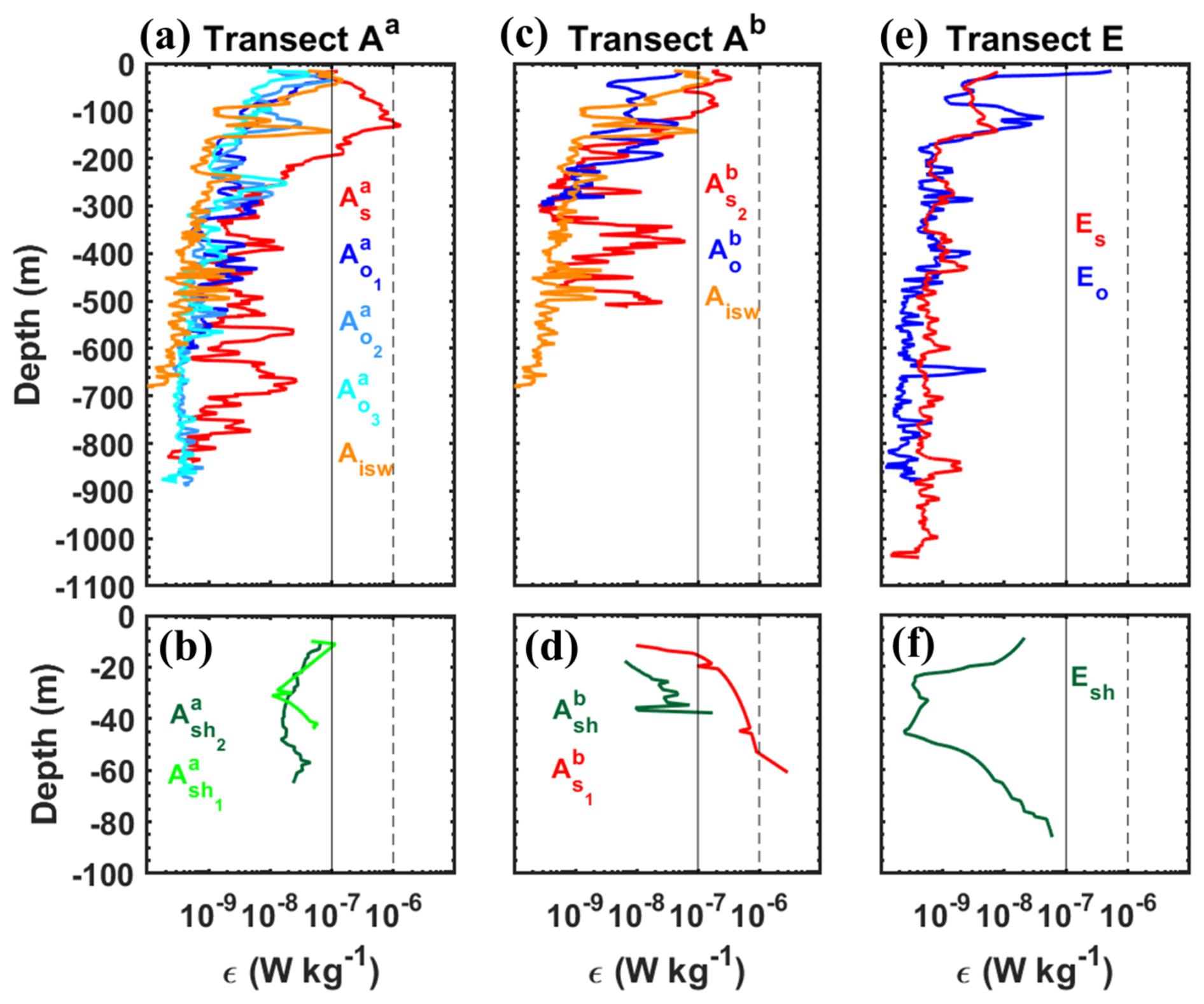
Figure 5 Station-averaged dissipation rate profiles (ε, in W kg⁻¹, logarithmic scale) from VMP measurements during the AMAZOMIX 2021 cruise along transects: (a, b) A^a, (c, d) A^b, and (e, f) E. Colored lines represent stations on the shelf (green, lime green), slope (red), and open ocean (blue, sky blue, cyan, and light orange). Vertical dashed and solid black lines are included for comparison.

Within the thermocline, the strongest ε values ([10⁻⁷, 10⁻⁶] W kg⁻¹) are measured at slope stations ($A_{{\mathrm{s}}_{\mathrm{1}}}^b$, $A_{{\mathrm{s}}_{\mathrm{2}}}^b$, and $A_{\mathrm{s}}^a$) of the HTE transects, whereas lower values ([10⁻⁹] W kg⁻¹) are recorded at station E_s (transect E). Elevated but relatively lower ε values ([10⁻⁸] W kg⁻¹) are detected at open-ocean stations (e.g., $A_{\mathrm{o}}^b$, $A_{{\mathrm{o}}_{\mathrm{2}}}^a$, and E_o) across all transects, except at station A_isw, where higher values ([10⁻⁷] W kg⁻¹) are observed (Fig. 5a, c, and e).

Below the thermocline, elevated ε values ([10⁻⁸] W kg⁻¹) persist at various depths at slope and open-ocean stations of the HTE transects (e.g., 375 and 503 m for $A_{{\mathrm{s}}_{\mathrm{2}}}^b$; 390, 562, and 668 m for $A_{\mathrm{s}}^a$; and 127 and 192 m for $A_{\mathrm{o}}^b$; Fig. 5a, c, and e), whereas on the LTE transect, there is no evidence of such hotspots of dissipation.

In the BBL, the highest ε values ([10⁻⁷] W kg⁻¹) are found below 35 m depth at slope and shelf stations ($A_{\text{sh}}^b$ and $A_{{\mathrm{s}}_{\mathrm{1}}}^b$) of transect A^b, while lower but still elevated values ([10⁻⁸] W kg⁻¹) are observed at shelf stations of transects A^a and E (Fig. 5b, d, and f). Note that, at the base of MLD (between 15–30 m depth), elevated ε values ($>{\mathrm{10}}^{-\mathrm{7}}$ W kg⁻¹) are found at slope stations $A_{\mathrm{s}}^a$ and $A_{{\mathrm{s}}_{\mathrm{2}}}^b$ and open-ocean stations $A_{{\mathrm{o}}_{\mathrm{2}}}^a$ and A_isw compared to other stations (Fig. 5a and c).

In summary, the vertical distribution of ε exhibits distinct spatial patterns across transects A^a, A^b, and E. Slope stations of the HTE transects A^a and A^b show higher values than those of the LTE transect E. Open-ocean stations generally display lower but still elevated values, except for station A_isw, which has higher ε. The HTE transects A^a and A^b consistently exhibit higher ε than the LTE transect E, which could emphasize the role of localized shear-driven mixing along IT paths, particularly in the open ocean. To further investigate the processes driving mixing, we analyze shear instability arising from current dynamics.

3.2 Processes contributing to mixing

In this subsection, we focus on the midwater layer, and we investigate the processes that might be responsible for the high mixing activity described in the previous section. In particular, we analyze the vertical structure of baroclinic currents and separate the contributions of baroclinic tidal currents and time-averaged currents (in the following mean currents) to dissipation.

3.2.1 Mean baroclinic current

First, we focus on the mean baroclinic current. Following the method described in Sect. 2.2.2 (Eqs. 1 and 5), the vertical structure of the mean circulation is examined through the along-shelf components of the time-averaged (mean) baroclinic velocities. Indeed, the along-shelf current is the dominant component of the mean circulation in the region, primarily driven by the NBC. Note that the analysis of cross-shelf components does not alter the results (figures not shown). For three contrasting long stations – two on the HTE transects ($A_{\mathrm{s}}^a$ and A_isw; Figs. 6a, b, and 8a) and one on the LTE transect (E_o; Figs. 7a, b, and 9a) – we show the vertical structure of the along-shelf mean baroclinic currents and the associated mean shear.

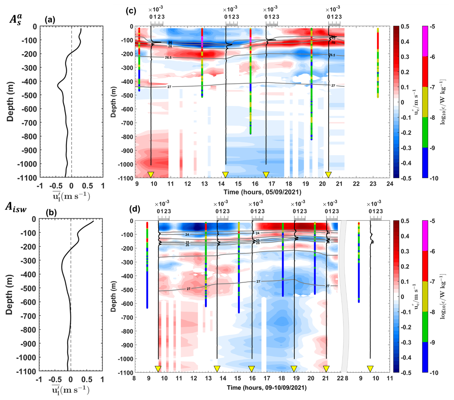
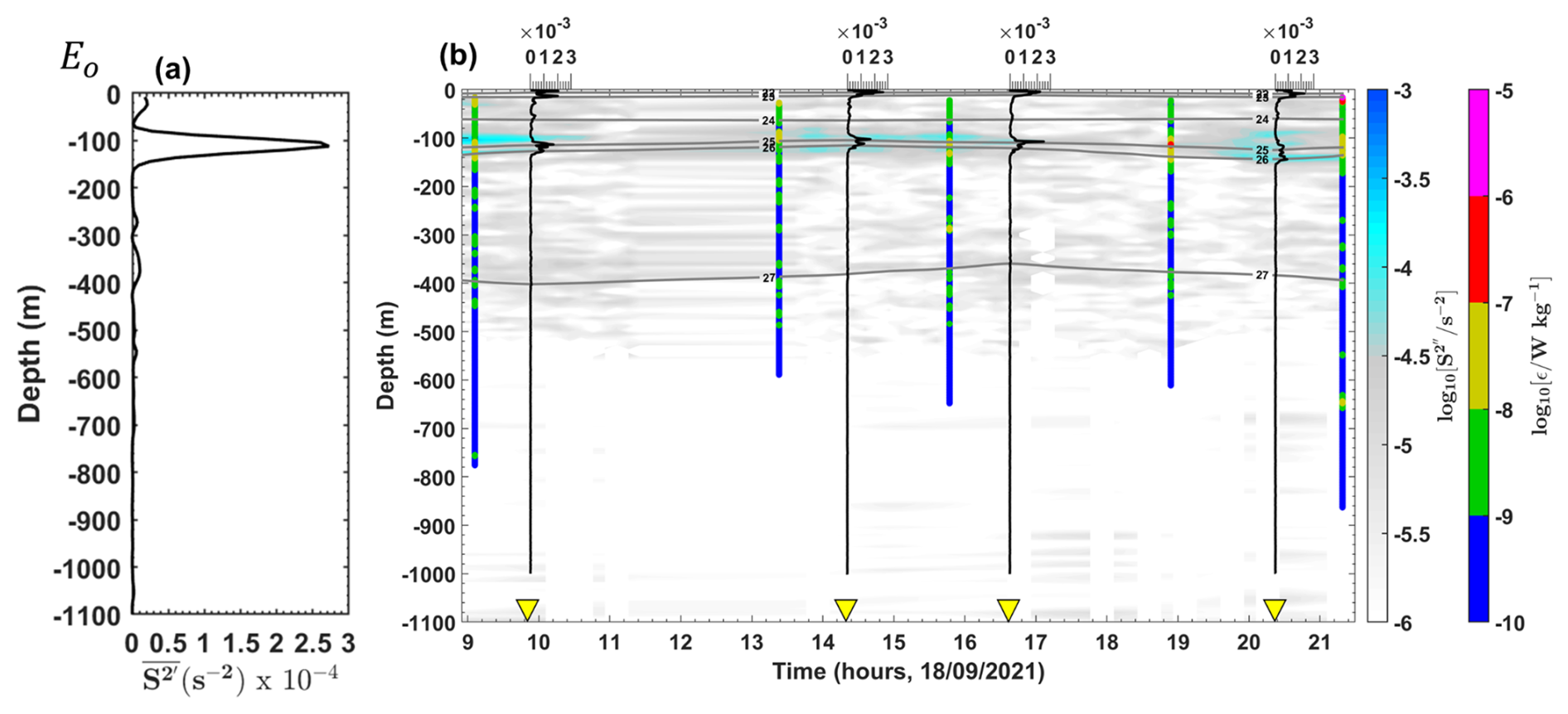
Figure 6 (a, b) Along-shelf mean baroclinic currents ($\stackrel{\mathrm{‾}}{{u^{\prime }}_{\mathrm{l}}}$, in m s⁻¹) and (c, d) cross-shelf semi-diurnal baroclinic currents (${u^{\prime \prime }}_{\mathrm{c}}$, in m s⁻¹) from the ADCP for stations (a, c) $A_{\mathrm{s}}^a$ and (b, d) A_isw. Panels (c) and (d) also show the buoyancy frequency squared (N², in s⁻²) as vertical black lines, potential density (σ_θ, kg m⁻³) as grey contours, and dissipation rate profiles (ε, in W kg⁻¹, logarithmic scale) as vertical colored bars. Yellow triangles mark the measurement times of CTD-O₂/LADCP profiles.

Figure 7 Panels follow the same format as in Fig. 6 but correspond to station E_o.

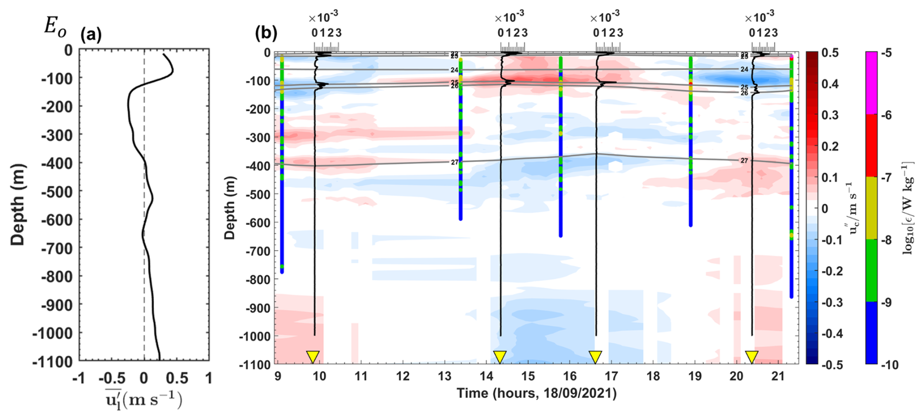
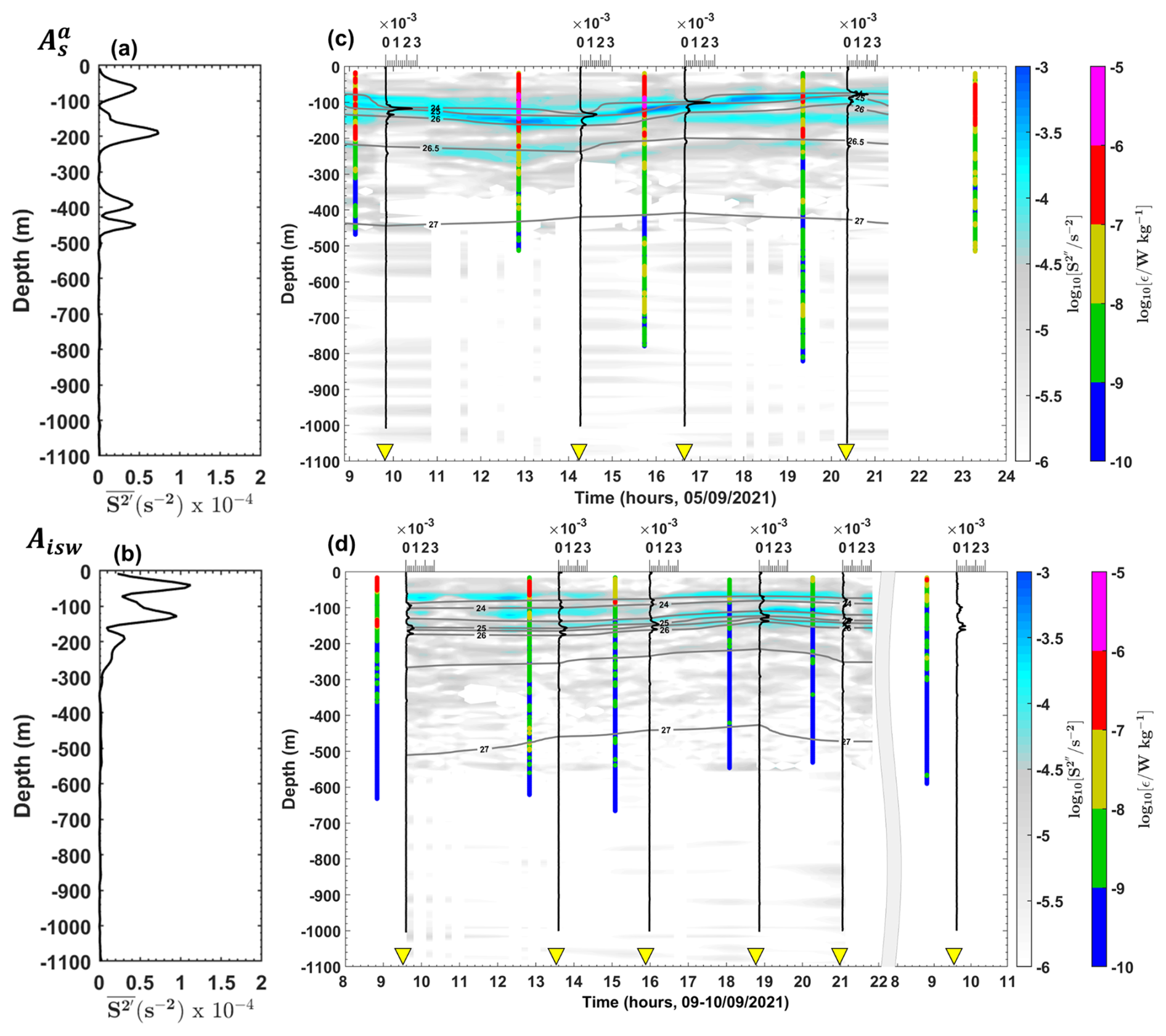
Figure 8 (a, b) Mean baroclinic vertical shear squared ($\stackrel{\mathrm{‾}}{S^{{\mathrm{2}}^{\prime }}}$, in s⁻²) and (c, d) semi-diurnal baroclinic vertical shear squared ($S^{{\mathrm{2}}^{\prime \prime }}$, in s⁻², logarithmic scale) from the ADCP for stations (a, c) $A_{\mathrm{s}}^a$ and (b, d) A_isw. Panels (c) and (d) also show the buoyancy frequency squared (N², in s⁻²) as vertical black lines, potential density (σ_θ, kg m⁻³) as grey contours, and dissipation rate profiles (ε, in W kg⁻¹, logarithmic scale) as vertical colored bars. Yellow triangles mark the measurement times of CTD-O₂/LADCP profiles.

Figure 9 Panels follow the same format as in Fig. 8 but correspond to station E_o.

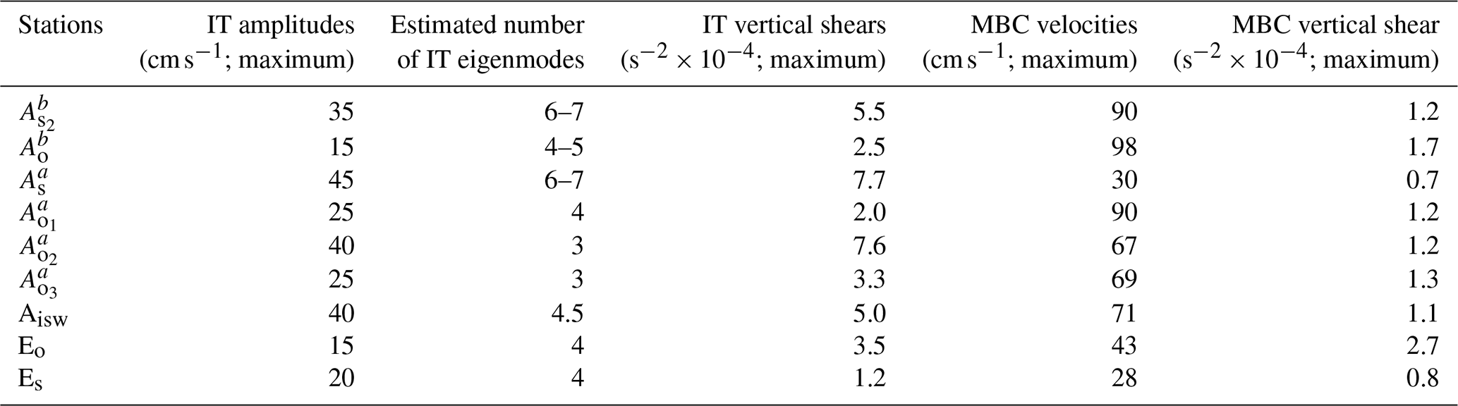
In the upper 200 m (referred to as the surface layer), a northwestward surface flow is observed at all stations except at E_s, where the flow direction is reversed to southeastward. Strong surface flow velocities (67–98 cm s⁻¹; Table C1, Appendix C) are recorded at all stations south of 3° N (e.g., at A_isw; Fig. 6b), except at $A_{\mathrm{s}}^a$, where velocities are reduced (∼30 cm s⁻¹; Fig. 6a). Strong vertical shear ($[\mathrm{1.1},\mathrm{1.7}]\times {\mathrm{10}}^{-\mathrm{4}}$ s⁻²; Table C1, Appendix C) is observed at stations south of 3° N (e.g., at A_isw; Fig. 8b), except at $A_{\mathrm{s}}^a$, where shear is weaker ([10⁻⁵] s⁻²; Fig. 8a) in the surface layer. At stations further north (above 4° N) in the surface layer, lower along-shelf velocities are noted for both northwestward (∼43 cm s⁻¹ at E_o; Fig. 7a) and southeastward flows (∼28 cm s⁻¹ at E_s; Table C1, Appendix C). Strong vertical shear ($\mathrm{2.7}\times {\mathrm{10}}^{-\mathrm{4}}$ s⁻² at E_o; Fig. 8a) is associated with the northwestward flow, while lower vertical shear ([10⁻⁵] s⁻² at E_s; Table C1, Appendix C) is observed for the southeastward flow. Below 200 m, a potential subsurface flow is identified between 200 and 700 m, particularly at stations south of 3° N (e.g., $A_{\mathrm{s}}^a$; Fig. 6a), with weak vertical shear ([10⁻⁵] s⁻²; Fig. 8a).

These findings suggest that the mean background circulation may play a substantial role in driving mixing mechanisms off the Amazon shelf.

3.2.2 Baroclinic tidal current

Second, we focus on baroclinic tidal currents. Following the method described in Sect. 2.2.2 (Eqs. 3 and 4), we examined the vertical structure of tidal currents using the cross-shelf components of semi-diurnal baroclinic velocities. The cross-shelf current is likely the dominant component of IT currents in the region. Note that the along-shelf velocity components were weaker than the cross-shelf components (figures not shown). For the same three contrasting long stations, we present time–depth sections of cross-shelf baroclinic tidal currents (Figs. 6c, d and 7b) and their associated tidal shear (Figs. 8c, d and 9b).

On the slope at $A_{\mathrm{s}}^a$, strong tidal current reversals occur approximately every 6 h within the pycnocline (70–180 m depth; 24–26 kg m⁻³ isopycnals; Fig. 6c), corresponding to the M₂ tidal component. These reversals reach amplitudes of up to 45 cm s⁻¹ (Fig. 6c) and vertically exhibit 6–7 alternating velocity peaks, indicating high vertical eigenmodes (modes 6–7; Fig. 6c). Similar conditions are observed at $A_{{\mathrm{s}}_{\mathrm{2}}}^b$, where tidal amplitudes reach 35 cm s⁻¹ (Table C1, Appendix C) with eigenmodes 6–7. In contrast, reduced amplitudes (20 cm s⁻¹) and slightly lower eigenmodes (mode 4) are recorded at E_s. In the open ocean at E_o, tidal currents are weaker (up to 15 cm s⁻¹; Fig. 7b) with eigenmodes around mode 4. Other open-ocean stations ($A_{{\mathrm{o}}_{\mathrm{1}}}^a$, $A_{{\mathrm{o}}_{\mathrm{3}}}^a$, and $A_{\mathrm{o}}^b$) show weak tidal amplitudes (15–25 cm s⁻¹; Table C1, Appendix C) and lower eigenmodes (modes 3–5). However, exceptions are noted at A_isw and $A_{{\mathrm{o}}_{\mathrm{2}}}^a$, where amplitudes remain high (40 cm s⁻¹; Table C1, Appendix C), particularly near the pycnocline.

On the slope, tidal vertical shear ranges between $[\mathrm{1.2},\mathrm{7.7}]\times {\mathrm{10}}^{-\mathrm{4}}$ s⁻². The strongest shear ($\mathrm{7.7}\times {\mathrm{10}}^{-\mathrm{4}}$ s⁻²; Fig. 8c) occurs at $A_{\mathrm{s}}^a$ within the pycnocline, while the weakest ($\mathrm{1.2}\times {\mathrm{10}}^{-\mathrm{4}}$ s⁻²; Table C1, Appendix C) is at E_s. In the open ocean, shear varies between $[\mathrm{2.0},\mathrm{7.6}]\times {\mathrm{10}}^{-\mathrm{4}}$ s⁻² (Table C1, Appendix C), with lower values ($\mathrm{3.5}\times {\mathrm{10}}^{-\mathrm{4}}$ s⁻²; Fig. 9b) at E_o. Exceptions again occur at A_isw and $A_{{\mathrm{o}}_{\mathrm{2}}}^a$, where baroclinic tidal shear remains relatively strong (between $[\mathrm{5.0},\mathrm{7.6}]\times {\mathrm{10}}^{-\mathrm{4}}$ s⁻²; Fig. 8d, Table C1, Appendix C), particularly near the pycnocline.

Along the slope, baroclinic tidal currents and shear are stronger along the HTE transects compared to LTE. In the open ocean, they are generally weaker, except at A_isw and $A_{{\mathrm{o}}_{\mathrm{2}}}^a$, where they remain high. These tidal currents and their associated shear coincide with strong vertical displacements of N² maxima (Sect. 3.1.1) and high dissipation rates (Sect. 3.1.2), raising the question of whether high mixing activity is primarily driven by IT or mean currents.

3.2.3 Competitive processes to generate mixing

Our aim in this subsection is to associate midwater mixing events with either baroclinic tidal currents or time-averaged (mean) currents. To achieve this, we map depth-integrated and maximum values of station-averaged ε and plot all ε values on a (time-mean shear $\stackrel{\mathrm{‾}}{S^{{\mathrm{2}}^{\prime }}}$, tidal shear $S^{{\mathrm{2}}^{\prime \prime }}$) diagram across five regions (A_s, A_o, A_isw, E_s, and E_o; Figs. 10 and 11). These regions are selected to contrast slope and open-ocean dynamics, with data included from the HTE and LTE transects. All data are collected from below the wind-influenced surface layer (defined as the maximum of XLD or MLD; see Sect. 2.2.1) and above the friction-dominated bottom boundary layer (H_BBL; defined in Sect. 2.2.1). Following the approach described in Sect. 2.2.2, we calculated the relative contributions of tidal shear and mean shear to the total baroclinic shear in order to quantify their role during each dissipation event.

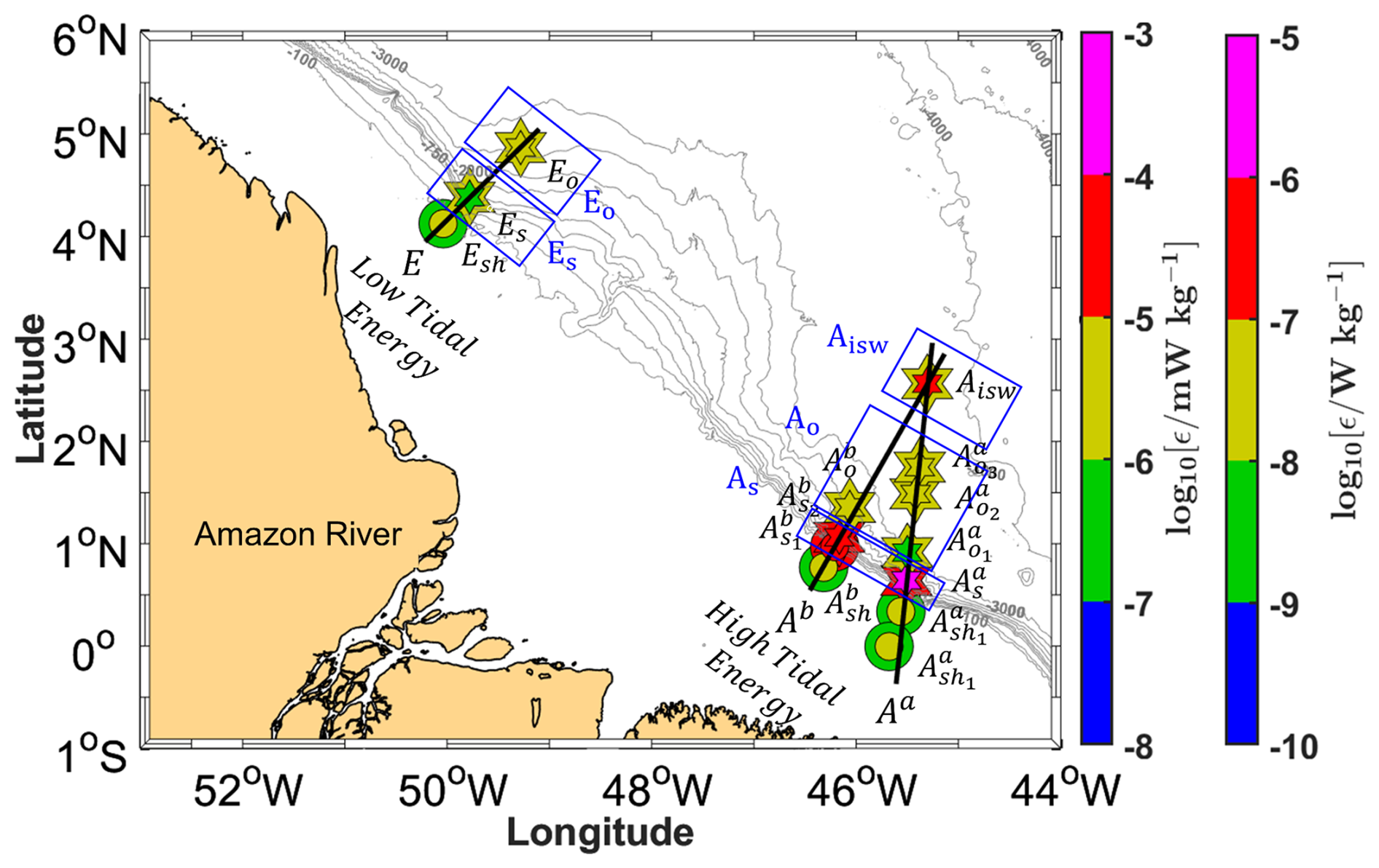
Figure 10 Depth-integrated (in mW kg⁻¹, logarithmic scale) and maximum values (in W kg⁻¹, logarithmic scale) of station-averaged dissipation rates (ε) from VMP measurements during the AMAZOMIX 2021 cruise. Solid black lines depict transects (A^a, A^b, and E) along high tidal energy (HTE) and low tidal energy (LTE) paths. Data are from below the wind-influenced surface layer and above the friction-dominated bottom boundary layer. Colored circles and stars represent short and long stations, respectively. Small and large colored circles indicate depth-integrated and maximum values of ε, respectively, with ranges shown by the color bar. Similarly, small and large colored stars indicate depth-integrated and maximum values of ε, respectively, with ranges shown by the color bar. Stations are grouped into five areas: A_s ($A_{\mathrm{s}}^a$ and $A_{{\mathrm{s}}_{\mathrm{2}}}^b$), A_o ($A_{\mathrm{o}}^b$, $A_{{\mathrm{o}}_{\mathrm{1}}}^a$, $A_{{\mathrm{o}}_{\mathrm{2}}}^a$, and $A_{{\mathrm{o}}_{\mathrm{3}}}^a$), A_isw (A_isw), E_s (E_s), and E_o (E_o). The five blue boxes indicate these defined areas. Subscripts denote locations: “s” for slope (A_s), “o” for offshore (A_o and E_o), and “isw” for ISW regions (A_isw).

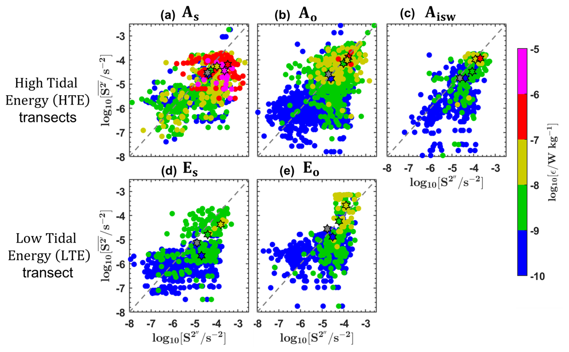
Figure 11 Dissipation rates (ε, in W kg⁻¹, logarithmic scale), measured below the wind-influenced surface layer (max [XLD, MLD]) and above the friction-dominated BBL (H_BBL), plotted as a function of the mean baroclinic vertical shear squared ($\stackrel{\mathrm{‾}}{S^{{\mathrm{2}}^{\prime }}}$, in s⁻², logarithmic scale) and semi-diurnal baroclinic vertical shear squared ($S^{{\mathrm{2}}^{\prime \prime }}$, in s⁻², logarithmic scale). Data are from defined areas: (a) A_s ($A_{\mathrm{s}}^a$ and $A_{{\mathrm{s}}_{\mathrm{2}}}^b$), (b) A_o ($A_{\mathrm{o}}^b$, $A_{{\mathrm{o}}_{\mathrm{1}}}^a$, $A_{{\mathrm{o}}_{\mathrm{2}}}^a$, and $A_{{\mathrm{o}}_{\mathrm{3}}}^a$), (c) A_isw (A_isw), (d) E_s (E_s), and (e) E_o (E_o). ε is represented by colored circles, with their ranges indicated on the color bar. Each panel also includes vertical shear averages for specific ε ranges ([10⁻⁶], [10⁻⁷], [10⁻⁸], [10⁻⁹], and [10⁻¹⁰] W kg⁻¹) depicted as colored stars with black edges, and grey stars with black edges represent the vertical shear averaged across all ε values. Dashed grey lines are included for comparison.

Dissipation hotspots ($\mathit{\epsilon }=[{\mathrm{10}}^{-\mathrm{6}},{\mathrm{10}}^{-\mathrm{7}}]$ W kg⁻¹; magenta and red circles in Figs. 11 and 10) are observed under strong vertical baroclinic shear ([10⁻⁴, 10⁻⁵] s⁻²), driven by either tidal or time-mean currents.

On the slope (A_s and E_s), high ε values in A_s are associated with stronger $S^{{\mathrm{2}}^{\prime \prime }}$ than $\stackrel{\mathrm{‾}}{S^{{\mathrm{2}}^{\prime }}}$ (magenta, red, and grey stars in Fig. 11a correspond to $S^{{\mathrm{2}}^{\prime \prime }}\approx {\mathrm{10}}^{-\mathrm{4}}>\stackrel{\mathrm{‾}}{S^{{\mathrm{2}}^{\prime }}}\approx {\mathrm{10}}^{-\mathrm{5}}$), indicating that tidal shear contributes ∼60 % to high ε values (Table B1, Appendix B). Similarly, in E_s, moderate ε values (yellow and grey stars in Fig. 11d) are primarily driven by tidal shear, which accounts for ∼60 % of the observed dissipation (Table B1, Appendix B).

In the open ocean (A_o, E_o, and A_isw), moderate ε values in A_o and E_o are found when $S^{{\mathrm{2}}^{\prime \prime }}$ is nearly equal to $\stackrel{\mathrm{‾}}{S^{{\mathrm{2}}^{\prime }}}$ (yellow, red, and grey stars in Fig. 11b and e correspond to $S^{{\mathrm{2}}^{\prime \prime }}\approx \stackrel{\mathrm{‾}}{S^{{\mathrm{2}}^{\prime }}}\approx {\mathrm{10}}^{-\mathrm{4}}$ s⁻²), suggesting tidal and time-mean shear each contribute ∼50 % to dissipation (Table B1, Appendix B). An exception is observed in A_isw, where high ε values coincide with slightly stronger tidal shear (red and grey stars in Fig. 11c correspond to $S^{{\mathrm{2}}^{\prime \prime }}\approx \mathrm{2}\times \stackrel{\mathrm{‾}}{S^{{\mathrm{2}}^{\prime }}}\approx \mathrm{2}\times {\mathrm{10}}^{-\mathrm{4}}$ s⁻²), suggesting that tidal shear contributes ∼60 % to dissipation hotspots (Table B1, Appendix B).

These results suggest that dissipation on the slope is slightly dominated by ITs, while offshore dissipation is equally balanced by mean circulation and ITs. However, exceptions exist in the open ocean, particularly at stations A_isw and $A_{\mathrm{o}}^b$, where tidal shear contributes ∼60 % and ∼30 % to dissipation, respectively. The dissipation at $A_{\mathrm{o}}^b$ is attributed to NBC. A key question remains: why does A_isw exhibit strong IT-driven dissipation ∼230 km from IT generation sites, with dissipation hotspots observed at various depths throughout the water column? To address this, we employ ray-tracing techniques to investigate potential IT propagation paths.

3.2.4 IT ray-tracing

In this subsection, IT ray paths are computed for the M₂ tidal frequency, following the method described in Sect. 2.2.3 (Eq. 6). These computations provide insights into linear theoretical energy flux paths in the vertical dimension (Rainville and Pinkel, 2006). The results are compared to previously estimated dissipation rates to explain the intense dissipation hotspot observed at A_isw, which contrasts with values typically found in the open ocean (Gille et al., 2012).

Figures 12 and 13 show that linear IT rays, derived from both model and observed density data, are generated at the critical slope near the 93 and 121 m isobaths on the HTE and LTE transects, respectively. After generation, the rays propagate downward through the water column, reflect at the seabed, and then propagate upward, where they are expected to reflect at the surface. This pattern continues seaward (Figs. 12 and 13). In reality, part of the IT beam may also reflect within the pycnocline. Surface reflections are observed at large distances from the ray generation sites: ∼105 and ∼230 km on transect A^a (Fig. 12a) and ∼100 and ∼220 km on transect A^b (Fig. 12b). These large distances may result from the greater orientation angle between the IT propagation direction and the transects. In contrast, surface reflections on transect E occur at shorter distances (∼80 and ∼205 km; Fig. 13), possibly due to eddy activity (Dossa et al., 2025). The linear rays suggest horizontal wavelengths of ∼90–125 km, consistent with mode-1 IT. Differences between transects may arise from variations in density, ocean depth, or angle between the IT propagation path and the transect orientation. The curvature of the rays becomes more pronounced as they interact with the pycnocline, particularly between 20 and 207 m depth, defined by the upper and lower thermocline depths (UTD and LTD; Figs. 12 and 13).

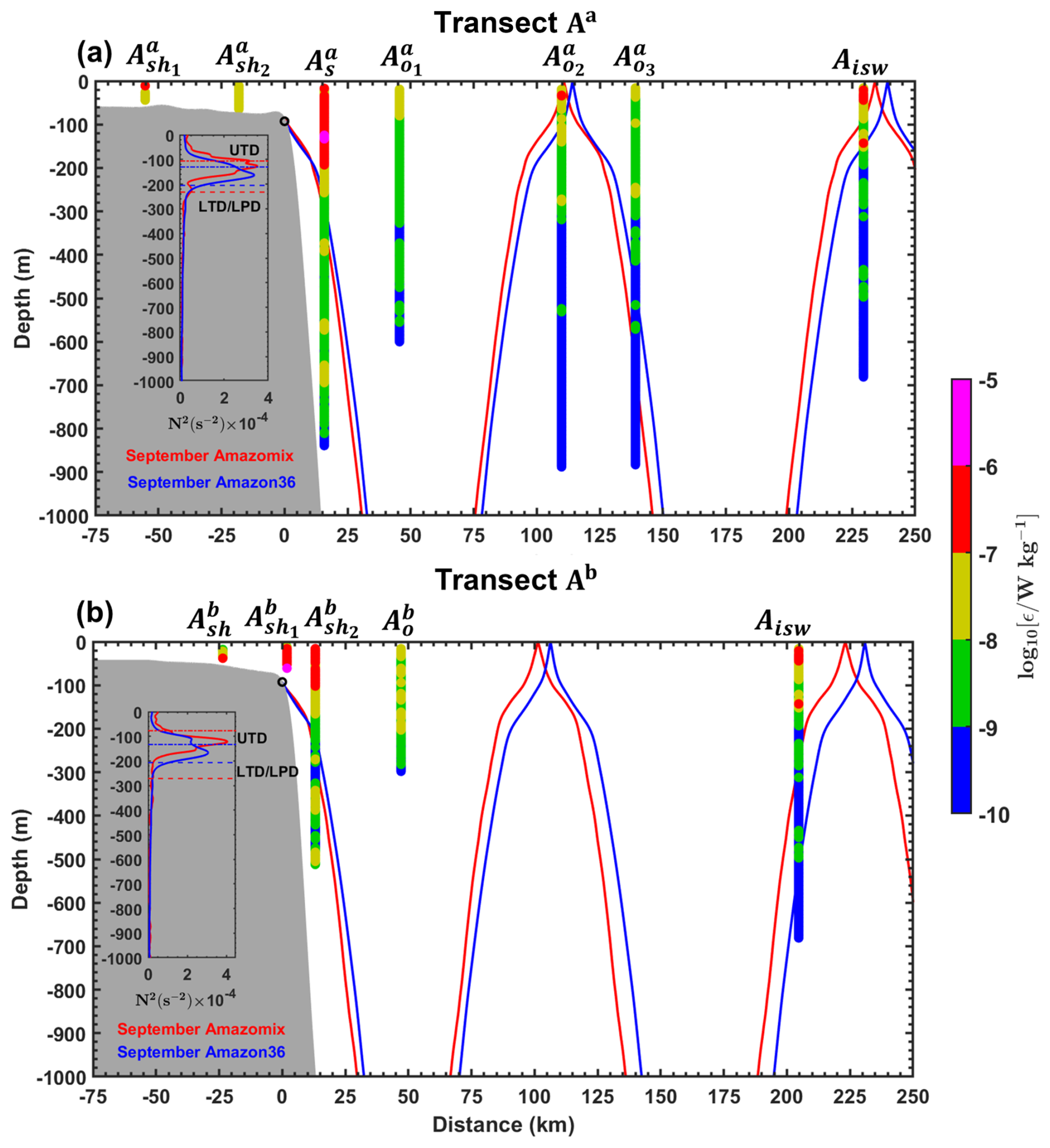
Figure 12 Ray-tracing diagrams for the M₂ constituent of IT along transects (a) A^a and (b) A^b. Ray calculations were performed using the mean buoyancy frequency squared (N², in s⁻²) derived from CTD-O₂ data (red ray) and NEMO-Amazon36 model data (blue ray) for September. Grey areas represent local topography, and black circles indicate the critical topography slopes (ray generation sites). Subpanels show N² profiles from AMAZOMIX (red line) and the NEMO-Amazon36 model (blue line), used for ray-tracing calculations. Upper thermocline depth (UTD, dotted lines) and lower thermocline/pycnocline depth (LTD/LPD, dashed lines) are also indicated in the subpanels.

Figure 13 Panels follow the same format as in Fig. 12 but correspond to transect E.

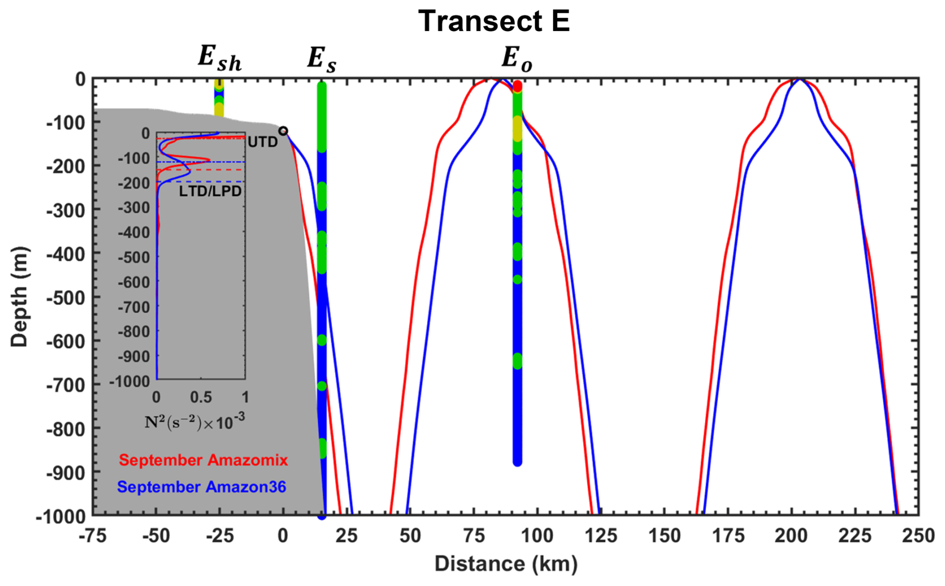
Tracking the IT rays along the transects reveals their possible alignment with dissipation hotspots (Figs. 12 and 13). On the slope, dissipation hotspots (between 60 and 180 m depth; Fig. 12a and b) at $A_{\mathrm{s}}^a$ and $A_{{\mathrm{s}}_{\mathrm{2}}}^b$ and around 15 km at the surface bounce likely result from nonlinear processes involving high-mode IT – such as IT breaking and shear instabilities – that are not captured by linear ray theory. In the open ocean, the surface dissipation (at 34 m depth; Fig. 12a) at $A_{{\mathrm{o}}_{\mathrm{2}}}^a$ may arise from surface reflections of the rays. Meanwhile, dissipation hotspots between 130 and 152 m depth at A_isw could result from either ray interference creating instabilities at multiple depths or the arrival of rays from transect A^a (at 87 and 150 m depth; Fig. 12a) and transect A^b (at 275 and 523 m depth; Fig. 12b) at A_isw.

4 Discussion and conclusion

The AMAZOMIX 2021 cruise provided, to the best of our knowledge, for the first time, direct measurements of turbulent dissipation using a VMP at multiple stations along contrasting IT paths. These measurements enabled the study of mixing processes at the Amazon shelf break and the adjacent open ocean. To capture a full tidal cycle, data on turbulent dissipation rates, hydrography, and currents were collected alternately over 12 h, with four to five profiles taken per station (see Sect. 2). The locations of the 12 h sampling stations were selected based on modeling results that provided realistic maps of IT generation, propagation and dissipation (Fig. 1; Tchilibou et al., 2022). Stations were located along the HTE paths A^a and A^b ($A_{{\text{sh}}_{\mathrm{1}}}^a{A}_{{\text{sh}}_{\mathrm{2}}}^a$, $A_{\mathrm{s}}^a$, $A_{{\mathrm{o}}_{\mathrm{1}}}^a$, $A_{{\mathrm{o}}_{\mathrm{2}}}^a$, $A_{{\mathrm{o}}_{\mathrm{3}}}^a$, A_isw, $A_{\text{sh}}^b$, $A_{{\mathrm{s}}_{\mathrm{1}}}^b$, $A_{{\mathrm{s}}_{\mathrm{2}}}^b$, and $A_{\mathrm{o}}^b$) and LTE path E (E_sh, E_s, and E_o).

4.1 Vertical displacements, homogeneous layers

First, step-like features were found in the density profile that characterized homogenized layers stacked atop one another, indicating intense mixing hotspots at various depths in the water column. Their vertical extent ranged between 4 and 41, consistent with step-like structures observed in other IT regions (Koch-Larrouy et al., 2015; Bouruet-Aubertot et al., 2018). Our results show that along the HTE paths (A^a and A^b), step-like structures were larger in the open ocean (up to 41 m) than over the slope (up to 10 m). In contrast, along the LTE path (E), they were smaller (4 m) and uniform across both the slope and open ocean, indicating weaker mixing.

Second, vertical isopycnal displacements ranged from 10 to 61 m, aligning with observations from other IT regions (Stansfield et al., 2001; Simpson and Sharples, 2012; Bordois, 2015; Koch-Larrouy et al., 2015; Zhao et al., 2016; Bouruet-Aubertot et al., 2018; Xu et al., 2020) that show a similar order of magnitude. On the HTE paths, the strongest displacements occurred over the slope (up to 58 m), with substantial variability in the open ocean (15–52 m). On the LTE path, displacements were weaker (24 m) and confined to the slope.

The differences between the open ocean and slope, as well as between HTE and LTE paths, are seemingly associated with IT propagation, which induces vertical displacements at tidal frequencies, promoting mixing and forming the step-like density features observed.

4.2 Direct measurements of dissipation rates

The station-averaged dissipation rate (ε) ranged from 10⁻¹⁰ to 10⁻⁶ W kg⁻¹, with distinct spatial patterns across paths A^a, A^b, and E. The highest ε values (10⁻⁷ to 10⁻⁶ W kg⁻¹) were observed at slope stations of the HTE paths, while lower ε values (10⁻⁹ W kg⁻¹) were found at slope stations of the LTE path (Fig. 14). Open-ocean ε values were generally lower (10⁻⁸ W kg⁻¹) but still elevated, especially at A_isw, where values reached 10⁻⁷ W kg⁻¹ near the pycnocline. The elevated ε near slopes on the HTE paths aligns with observations from other energetic IT generation sites (e.g., the Hawaiian Ridge, Klymak et al., 2008; Halmahera Sea, Koch-Larrouy et al., 2015; Bouruet-Aubertot et al., 2018). In contrast, lower ε values near slopes on the LTE path are comparable to those in less energetic IT regions (e.g., Takahashi and Hibiya, 2019). In the open ocean, ε values – though lower than slope measurements – remain elevated, particularly at A_isw, where they exceed typical background levels (10⁻¹⁰–10⁻⁸ W kg⁻¹; e.g., Southern Ocean, Gille et al., 2012; Banda Sea, Bouruet-Aubertot et al., 2018). This suggests localized turbulent dissipation, likely driven by ITs or mesoscale currents.

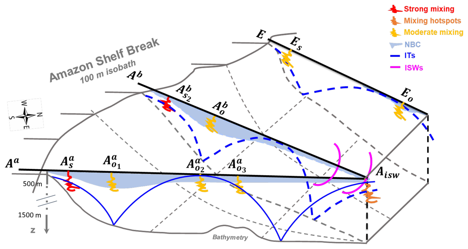
Figure 14 Summary diagram illustrating the key processes driving mixing across the HTE paths (A^a and A^b) and LTE path (E) off the Amazon shelf. At IT generation sites (stations $A_{\mathrm{s}}^a$, $A_{{\mathrm{s}}_{\mathrm{2}}}^b$, and E_s), mixing is generally stronger (red zigzags), except at E_s, where it is moderated (yellow zigzags). At these generation sites, ITs contribute ∼60 % to mixing, exceeding the contribution of the mean circulation (NBC). Away from generation sites in the open ocean (e.g., $A_{\mathrm{o}}^b$, $A_{{\mathrm{o}}_{\mathrm{1}}}^a$, and E_o; yellow zigzags), mixing decreases but remains substantial, driven by nearly equal contributions from ITs and mean circulation. A key observation is the increased mixing ∼230 km from the generation sites, forming a hotspot at A_isw (orange zigzags). This coincides with the surfacing of IT rays (blue lines) from two distinct generation sites on the HTE paths, the vanishing of the NBC (sky-blue shaded areas), and the presence of ISWs (magenta lines). These observations suggest that constructive interference of IT rays may generate ISWs, amplifying mixing at A_isw.

4.3 Enhanced dissipation at the base of the MLD

Near the base of the MLD (15–30 m depth), high ε values ($>{\mathrm{10}}^{-\mathrm{7}}$ W kg⁻¹) were observed at slope stations ($A_{\mathrm{s}}^a$ and $A_{{\mathrm{s}}_{\mathrm{2}}}^b$) and open-ocean stations ($A_{{\mathrm{o}}_{\mathrm{2}}}^a$ and A_isw) along the HTE paths. These findings agree with model results from Tchilibou et al. (2022) and Assene et al. (2024), which identified similar near-surface ε hotspots in the HTE regions.

4.4 Contribution of background circulation and ITs to mixing

To identify the processes driving the observed high mixing activity, we analyzed shear instabilities in both mean and semi-diurnal baroclinic currents and quantified their relative contributions to mixing.

4.4.1 Mean baroclinic current shear

First, we analyzed the along-shelf component of the mean baroclinic current (MBC) as it dominates the mean circulation in the region. MBC was primarily observed in the surface layer (0–200 m depth), driven by a northwestward flow with strong velocities (67–98 cm s⁻¹) and shear instability (between $[\mathrm{1.1},\mathrm{1.7}]\times {\mathrm{10}}^{-\mathrm{4}}$ s⁻²) at all stations south of 3° N. This flow is associated with the NBC, which moves northwestward along the Brazilian coast (Johns et al., 1998; Bourlès et al., 1999). However, at slope station $A_{\mathrm{s}}^a$, NBC velocities were lower (∼30 cm s⁻¹) with weak NBC vertical shear ($\sim {\mathrm{10}}^{-\mathrm{5}}$ s⁻²), likely due to topographic effects that weaken NBC near the continental slope (da Silveira et al., 1994). Further north (above 4° N), the surface layer exhibited weak MBC with low shear instability ($\sim {\mathrm{10}}^{-\mathrm{5}}$ s⁻²) in the open ocean, except near the slope, where MBC reversed to southeastward with strong shear ($\mathrm{2.7}\times {\mathrm{10}}^{-\mathrm{4}}$ s⁻²). This reversal could be related to subsurface eddy activity (Dossa et al., 2025) and the retroflection of the NBC, both common features in the region (Fratantoni and Glickson, 2002). Below the surface layer (200–700 m depth), a potential southeastward flow beneath the NBC was observed, with weak shear instability ($\sim {\mathrm{10}}^{-\mathrm{5}}$ s⁻²), particularly near the slope south of 3° N (e.g., at $A_{\mathrm{s}}^a$). This flow may be associated with a subsurface countercurrent (Dossa et al., 2025).

4.4.2 IT shear

Second, the semi-diurnal (M₂) baroclinic currents were extracted from the total baroclinic current, revealing pronounced IT signatures and associated tidal shear on the slope compared to the open ocean. Tidal amplitudes, eigenmodes, and shear were stronger along the HTE paths compared to the LTE path. At slope stations on the HTE paths, tidal amplitudes were high (35–45 cm s⁻¹) with dominant modes 6–7, whereas at slope stations on the LTE path, amplitudes were reduced (20 cm s⁻¹) with mode 4. In the open ocean, tidal amplitudes and modes were generally lower (15–25 cm s⁻¹; modes 3–5), except at A_isw and $A_{{\mathrm{o}}_{\mathrm{2}}}^a$, where amplitudes remained elevated (40 cm s⁻¹), particularly near the pycnocline. Vertical shear associated with baroclinic tidal currents was also stronger along the HTE paths, with values of 5.5–$\mathrm{7.7}\times {\mathrm{10}}^{-\mathrm{4}}$ s⁻² at slope stations compared to $\mathrm{1.2}\times {\mathrm{10}}^{-\mathrm{4}}$ s⁻² along the LTE path. In the open ocean, shear values were generally weaker (2.0–$\mathrm{3.5}\times {\mathrm{10}}^{-\mathrm{4}}$ s⁻²), except at A_isw and $A_{{\mathrm{o}}_{\mathrm{2}}}^a$, where they remained high (5.0–$\mathrm{7.6}\times {\mathrm{10}}^{-\mathrm{4}}$ s⁻²), particularly around the pycnocline. Strong IT signals – observed in amplitudes, modes, and associated shear – near slopes along the HTE paths align with measurements at other generation sites (e.g., Hawaiian Ridge, Zhao et al., 2016; Ombai Strait and Halmahera Sea, Bouruet-Aubertot et al., 2018). In contrast, slightly weaker IT signals near slopes along the LTE path are consistent with observations from regions of low IT activity (e.g., Banda Sea, Bouruet-Aubertot et al., 2018). Offshore, IT signals are typically weak, consistent with areas distant from generation sites (e.g., Halmahera Sea, Bouruet-Aubertot et al., 2018), except at stations A_isw and $A_{{\mathrm{o}}_{\mathrm{2}}}^a$, where there are IT signal hotspots.

These results suggest that shear instabilities–driven by the mean flow and IT-may lead to mixing off the Amazon shelf, raising the question of whether MBC or IT dominates the mixing process.

4.4.3 IT $/$ MBC ratio

Through direct quantification, we determined the relative contributions of MBC and IT to mixing. The results showed that both IT and MBC shear contribute to mixing, with their relative dominance varying across the HTE paths and LTE path. Near generation sites at slope stations ($A_{\mathrm{s}}^a$, $A_{{\mathrm{s}}_{\mathrm{2}}}^b$, and E_s), IT shear dominated the IT $/$ MBC shear ratio, contributing approximately ∼60 % to mixing. At open-ocean stations farther from generation sites (e.g., at $A_{{\mathrm{o}}_{\mathrm{2}}}^a$, $A_{{\mathrm{o}}_{\mathrm{3}}}^a$, and E_o), the contributions were nearly balanced, with each contributing around 50 %. Exceptions in the open ocean were observed at station A_isw, where IT shear became dominant again (contributing ∼60 %), and at station $A_{\mathrm{o}}^b$, where IT shear contribution decreased to ∼30 %. These results show that strong mixing near IT generation sites is primarily driven by IT shear instability, coherent with other sites (Klymak et al., 2008; Koch-Larrouy et al., 2015; Bouruet-Aubertot et al., 2018). Offshore, weaker mixing along IT paths is due to both IT and mean flow shear instability. This reduced mixing could result from ITs interacting with background flows, which advect energy away, or from effective offshore radiation (Whalen et al., 2012). At $A_{\mathrm{o}}^b$, away from generation sites, the lower IT shear contribution to mixing was attributed to the strong influence of the MBC, dominated by the NBC.

The most relevant finding of this study was an increased mixing near the pycnocline layer, which surfaces at A_isw in the open ocean. This supports the results of Assene et al. (2024) and de Macedo et al. (2025).

4.5 Unexpected strong open-ocean dissipation at A_isw

Along the HTE paths at station A_isw, elevated remote dissipation rates ($\sim {\mathrm{10}}^{-\mathrm{7}}$ W kg⁻¹) were detected ∼230 km from the shelf break. This region has been modeled as a surface-reaching IT dissipation hotspot (Tchilibou et al., 2022; Assene et al., 2024), driving sea surface temperature cooling (Assene et al., 2024). Observations also link this area to chlorophyll blooms (de Macedo et al., 2025; M'hamdi et al., 2025) and the generation of large-amplitude (>100 m) nonlinear IT-induced ISWs (Brandt et al., 2002; de Macedo et al., 2023).

Our key findings quantify dissipation hotspots in the water column at A_isw, including intensified dissipation at the mixed-layer base, providing in situ validation for prior model hypotheses (Tchilibou et al., 2022; Assene et al., 2024). We further propose that IT disintegration into nonlinear, more dissipative baroclinic flux may occur here. At A_isw, IT rays from two distinct generation sites (A^a and A^b) surface alongside documented ISWs, coinciding with the vanishing point of NBC. This interaction zone may foster constructive interference of IT rays, potentially creating higher tidal modes (New and Pingree, 1992; Silva et al., 2015; Barbot et al., 2021; Solano et al., 2023). Such modes could enhance nonlinear ISW generation (e.g., Jackson et al., 2012) and explain the observed elevated dissipation rates (Xie et al., 2013).

Appendix A

The AMAZOMIX measurement sites and stations were systematically named and organized by location. Each site received a unique identifier based on its position along the HTE and LTE paths. Stations were categorized by site and region: superscripts “a” and “b” denoted stations at sites A^a and A^b, respectively, while subscripts indicated location – “sh” for shelf, “s” for slope, “o” for offshore/open ocean, and “isw” for ISW regions (Table A1). This structured naming system ensured clear identification and logical grouping of stations for consistent data analysis.

Table A1 The naming system of the AMAZOMIX cruise measurement sites and stations.

Appendix B

To relate each mixing event with either tidal or mean (time-averaged) currents along the HTE transects (A^a and A^b) and the LTE transect (E), we quantify the relative contributions of mean and semi-diurnal baroclinic vertical shear squared at transect stations (see Table B1).

Table B1 Mixing layer depth (XLD), mixed layer depth (MLD), and contribution (mean and standard deviation) of the semi-diurnal (CSBS) and mean baroclinic (CMBS) shear to total baroclinic shear.

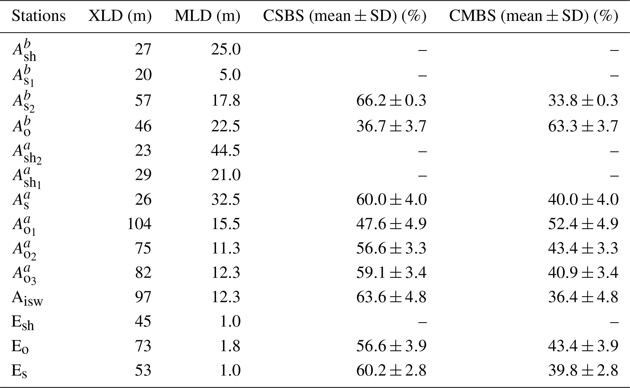
SD = standard deviation.

Appendix C

Following Sect. 2.2.2, we examine the cross-shelf component of baroclinic tidal currents to investigate IT amplitude (current strength) and shear instability around the pycnocline (70–180 m depth; see Table C1). Additionally, the along-shelf component of mean baroclinic currents (MBC) was analyzed to evaluate the strength of the mean flow and its associated shear instability in the upper 200 m (see Table C1).

Table C1 Strength of baroclinic tidal and mean baroclinic currents.