Relating Atlantic meridional deep-water transport to ocean bottom pressure variations as a target for satellite gravimetry missions

The Atlantic Meridional Overturning Circulation (AMOC) is a salient feature of the climate system that is observed with respect to its strength and variability using a wide range of offshore installations and expensive sea-going expeditions. Satellite-based measurements of mass changes in the Earth system, such as from the Gravity Recovery and Climate Experiment (GRACE) mission, may help monitor these transport variations at the large scale, by measuring associated changes in ocean bottom pressure (OBP) at the boundaries of the Atlantic remotely from space. However, as these signals are mainly confined to the continental slope and are small in magnitude, their detection using gravimetry will likely require specialised approaches. Here, we use the output of a fine-resolution ($\mathrm{1}/\mathrm{20}$°) regional ocean model to assess the connection between OBP signals at the western boundary of the North and South Atlantic to changes in the zonally integrated meridional deep-water transport. We find that transport anomalies in the ∼ 1–3 km depth range can be reconstructed using OBP variations spatially averaged over the continental slope, with correlations of 0.75 (0.72) for the North (South) Atlantic and root-mean-square errors of ∼ 1 Sv (sverdrup; 10⁶ m³ s⁻¹), on monthly to inter-annual timescales. We further create a synthetic data set containing OBP signals connected to meridional deep-water-transport anomalies; these data can be included in dedicated satellite gravimetry simulations to assess the AMOC detection capabilities of future mission scenarios and to develop specialised recovery strategies that are needed to track those weak signatures in the time-variable gravity field.

1 Introduction

The Atlantic Meridional Overturning Circulation (AMOC) is a defining element of the three-dimensional ocean general circulation and comprises a fine-structured system of currents. In aggregate, the upper overturning cell transports warm water masses in the near-surface layers of the Atlantic northward. In the Labrador Sea and Nordic Seas, comparatively dense water masses are formed by deep convection and overflows, respectively. The resulting deep-water mass, the so-called North Atlantic Deep Water (NADW), is subsequently transported southward for reasons of continuity and rises in the Southern Ocean (Buckley and Marshall, 2016), e.g. in the Antarctic divergence. Additionally, there is a deep overturning cell that contributes to the AMOC and is associated with the transport of Antarctic Bottom Water (AABW). AABW is formed in the Southern Ocean close to Antarctica, e.g. in the Weddell and Ross seas, where cold and salty water masses are produced and form the deepest water masses in the ocean. Part of the AABW then flows northward along the ocean floor initially west of the Mid-Atlantic Ridge (Lozier, 2010; McCarthy et al., 2020).

Whereas the detailed role of the AMOC in climate change scenarios is still debated, evidence suggests that the AMOC has not only a regional impact on the North Atlantic but also global consequences (Collins et al., 2022). Over the past decades, this has motivated numerous sea-going campaigns and long-term observation arrays to measure variations in meridional transports at various latitudes in the North and South Atlantic (Frajka-Williams et al., 2019; McCarthy et al., 2020), most notably the RAPID array. While these in situ measurements are certainly the most direct approach to monitor the AMOC, they come with significant annual operational costs; therefore, measurement arrays are still relatively sparse.

Instead, using basin-wide measurement arrays, zonally integrated meridional volume transport (MVT) variations can also be inferred through the measurement of ocean bottom pressure (OBP) variations at the sloped lateral boundaries of the Atlantic Basin alone. Under the geostrophic approximation, meridional transport variations can be determined through the difference between the eastern and western boundary pressure. In fact, as shown by Bingham and Hughes (2008), the western pressure signals alone are sufficient to capture almost all of the geostrophic transport variations at 42° N on inter-annual timescales. This physical connection offers the prospect of determining AMOC variations through satellite gravimetry measurements such as those from the Gravity Recovery and Climate Experiment (GRACE) mission (Tapley et al., 2004) and the Gravity Recovery and Climate Experiment Follow-on (GRACE-FO) mission (Landerer et al., 2020), which measure large-scale OBP changes globally at a monthly resolution.

Some success with this approach has indeed been reported by Landerer et al. (2015), who used JPL RL05 GRACE mascon solutions to determine Lower North Atlantic Deep Water (LNADW, depths of 3–5 km) transports at 26.5° N over the 2003–2014 period. The authors found good agreement with in situ measurements from the RAPID array at the very same latitude. These results were met with scepticism by Hughes et al. (2018), who suggested that the transports inferred by Landerer et al. (2015) were not necessarily associated with the western continental slope dynamics. While it may be that the smoothing effect of GRACE measurements allows for the detection of transport-related, spatially coherent OBP signals, studies have indicated that MVT-related OBP anomalies are confined to the narrow continental slope only (Bingham and Hughes, 2008; Roussenov et al., 2008; McCarthy et al., 2020).

There are, however, two considerations that motivate further studies of GRACE-based AMOC variability. Firstly, all attempts so far have relied on “standard” global monthly gravity field solutions, which are in no way tuned for the detection of the narrow OBP signals along the continental slope. Specific, tailored approaches, such as gravity field inversions with averaging times other than monthly or spatial constraints emphasising the continental slope, may lead to better signal-to-noise ratios for the OBP signals caused by AMOC variations. Secondly, several space agencies are currently preparing new satellite gravimetry missions such as the Gravity Recovery and Climate Experiment Continuity (GRACE-C) mission (by NASA and DLR with an expected launch in 2028) and the Next Generation Gravity Mission (NGGM; planned by ESA for 2032), which together will form the Mass-Change and Geosciences International Constellation (MAGIC). MAGIC offers the prospect of resolving much smaller spatial scales than previously accessible from GRACE alone (Pail et al., 2015). Preliminary analyses of the capabilities of MAGIC show that the increase in resolution may be sufficient to capture MVT-related boundary pressure signals in the North Atlantic (Daras et al., 2024). The MAGIC mission requirements document indicates a target resolution and accuracy of 100 km and 1.5 cm equivalent water height at monthly timescales (Haagmans and Tsaoussi, 2020), but detailed end-to-end simulations with the final mission configuration are still to be performed in the near future.

Therefore, we propose to pursue a more thorough assessment of the capabilities of current and future satellite gravimetry missions to monitor AMOC transport variability. In the present work, we analyse the connection between MVT and OBP anomalies between 1000 and 3000 m depth in a high-resolution general circulation model focusing on the North and South Atlantic. We explore how the modelled OBP variations associated with geostrophic MVT can be synthesised in preparation of dedicated end-to-end simulation studies of satellite gravimetry. This, in turn, will allow future studies to design suitable geodetic processing strategies (considering, e.g. various noise contributors including ocean tides) or to assess planned future mission scenarios such as MAGIC. We limit our analyses to periods below 5 years, corresponding to the nominal mission lifetime of gravity missions in low-altitude orbits.

2 Methods

2.1 Inferring MVT variations from OBP

Meridional transports can be related to boundary pressure based on the zonal momentum equation under geostrophic approximation as follows (Roussenov et al., 2008):

$$\begin{array}{}\text{(1)}& fv={\displaystyle \frac{\mathrm{1}}{{\mathit{\rho }}_{\mathrm{0}}}}{\displaystyle \frac{\partial p}{\partial x}},\end{array}$$

where v represents the meridional geostrophic velocity; p is pressure; f=2Ωsin ϕ is the latitude-dependent Coriolis parameter, which depends on Earth's rotational frequency Ω; and ρ₀ the reference density. Integrating in the zonal (x) direction over the entire Atlantic Basin gives the meridional geostrophic transport T:

$$\begin{array}{}\text{(2)}& T(y,z)=\int v\mathrm{d}x={\displaystyle \frac{p_{\mathrm{E}}(y,z)-p_{\mathrm{W}}(y,z)}{f{\mathit{\rho }}_{\mathrm{0}}}},\end{array}$$

where p_E (p_W) is the eastern (western) boundary pressure. As highlighted by Bingham and Hughes (2008), the transport variations in the upper (lower) limb can be reconstructed from western boundary pressures with a skill of 92 % (96 %). As a result, measurements of only the western boundary pressure from in situ recorders (or satellite gravimetry) may be used to infer anomalies of meridional transports via the following expression:

$$\begin{array}{}\text{(3)}& T^{\prime }(y,z)\approx -{\displaystyle \frac{p_{\mathrm{W}}^{\prime }(y,z)}{f{\mathit{\rho }}_{\mathrm{0}}}}.\end{array}$$

The prime notation that we use here indicates that only anomalies are considered, as the absolute transports are not accessible without knowledge of the eastern boundary signals. Instead of the transport at a certain depth, the total transport anomaly over a given depth range can be determined by vertical integration. For the transport anomalies that we focus on here, this gives the following:

$$\begin{array}{}\text{(4)}& T_{\mathrm{MVT}}^{\prime }\left(y\right)\approx -\underset{\mathrm{3000}\mathrm{m}}{\overset{\mathrm{1000}\mathrm{m}}{\int }}{\displaystyle \frac{p_{\mathrm{W}}^{\prime }(y,z)}{f{\mathit{\rho }}_{\mathrm{0}}}}\mathrm{d}z.\end{array}$$

$T_{\mathrm{MVT}}^{\prime }$ now represents the zonally integrated meridional volume transport anomalies. While NADW transport variations are likely a major contributor to these anomalies, there are other water masses involved when considering basin-wide transports. To remain general enough in our terminology, we will simply refer to MVT below.

Implicit to the above considerations are several simplifying assumptions. Firstly, we are presuming that geostrophic balance holds for these large-scale flows, especially when integrating zonally through the Deep Western Boundary Current. As long as the boundary current is narrow and oriented in a north–south direction, the impact of non-geostrophic terms should be minimal (Bingham and Hughes, 2008). In addition, as frictional terms are neglected in the above framework, we cannot trace transport variations in the Ekman layer. Bottom friction can only be neglected when the sidewalls of the basin are sufficiently steep (Little et al., 2019). Secondly, ignoring contributions from the eastern boundary means that the net MVT as well as OBP variations that are homogeneous across the basin are inaccessible (e.g. Stepanov and Hughes, 2006). Despite these limitations, several simulation studies have confirmed the tight connection between the western boundary pressure and MVT variations (Bingham and Hughes, 2008; Roussenov et al., 2008; Bingham and Hughes, 2009).

Because we are interested in inferring variations in the upper overturning cell, there are two water masses to consider. Typically, the overturning at a given latitude is taken to be the maximum of the streamfunction at that particular latitude (McCarthy et al., 2020) and, thus, comprises the northward-flowing upper layer of the ocean up to a depth of about 1000 m. OBP variations associated with this upper limb of the AMOC can, therefore, only be sensed in areas shallower than this threshold, which is the continental shelf region. Alternatively, changes in the overturning can be quantified by variations in the southward-flowing limb at depths below 1000 m and extending as deep as 5000 m (Send et al., 2011), which is, to a good degree, associated with NADW transport anomalies. For this deeper MVT, western boundary pressure variations are found primarily along the continental slope that connects shelf and deep-ocean regions. In principle, both of these approaches should yield equivalent results, as the northward and southward mass transports of the upper overturning cell mostly compensate for the North Atlantic, as shown by studies such as Bingham and Hughes (2008). In the South Atlantic, the flow of AABW somewhat complicates the relation between the northward and southward limb of the upper overturning cell, meaning that the southward return transport does not equal the maximum of the streamfunction anymore.

However, an advantage of considering OBP variations along the continental slope is that the overall variability in OBP in the slope region is significantly smaller than that of the adjoining deep-ocean and continental shelf areas, where either eddy activity or wind-driven circulations dominate (see Fig. 1). Thus, we expect transport-induced variations to make up a larger percentage of the total variability on the continental slope compared to the shelf area. However, this also means that the OBP signals are of a very small horizontal extent, which poses a challenge with respect to detecting them in satellite gravimetry observations.

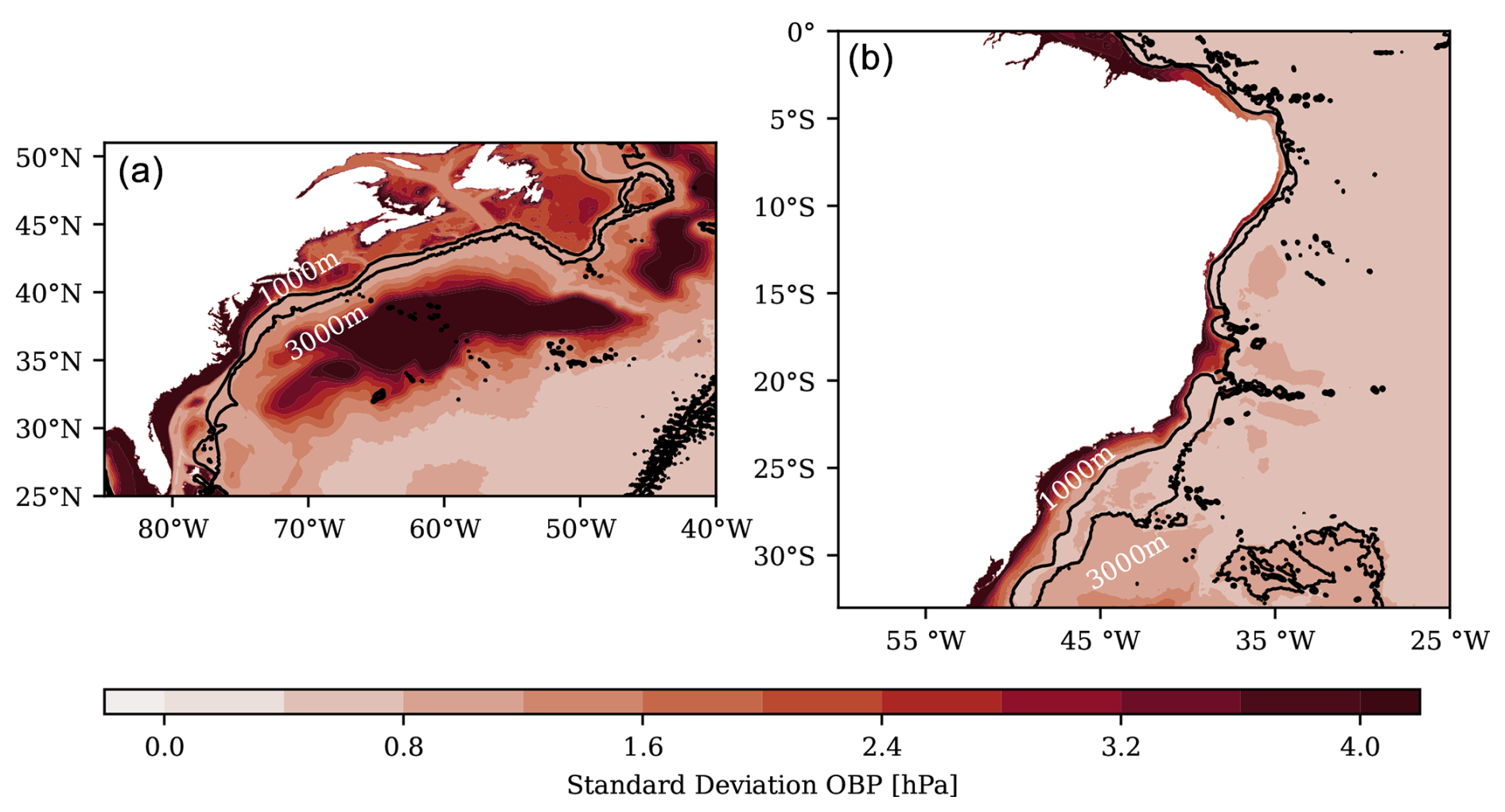
Figure 1 Standard deviation in the ocean bottom pressure (OBP) from VIKING20X for parts of the North Atlantic (a) and South Atlantic (b). The 1000 and 3000 m isobaths are shown as contour lines indicating the continental slope region.

2.2 Ocean model

In this study, we rely on simulations with the ocean–sea ice model VIKING20X, which is based on the NEMO3.6 ocean (Madec et al., 2023) and LIM2 sea ice (Fichefet and Maqueda, 1997) models being executed on the global eddy-permitting ORCA025 tripolar Arakawa-C grid with a nominal resolution of 0.25°. VIKING20X features regional refinement for the Atlantic Ocean from 33.5° S to about 65° N with a nominal horizontal resolution of $\mathrm{1}/\mathrm{20}$° and applies two-way nesting by means of Adaptive Grid Refinement in Fortran (AGRIF; Debreu et al., 2008), which enables an eddy-rich simulation in this specified area. Both the global low-resolution and regional high-resolution grids consist of 46 vertical z layers. The high horizontal resolution in the Atlantic is well suited for the investigation of the boundary pressure changes along the narrow western continental slope. The model run that we employ here, VIKING20X-JRA-OMIP, internally named VIKING20X.L46-KFS003 (Biastoch et al., 2021), extends from 1958 to 2019 and applies JRA55-do atmospheric forcing (Tsujino et al., 2018). From the model output, we derive the Atlantic meridional overturning streamfunction by zonally and vertically integrating the daily mean meridional velocity component. OBP is computed using the cdfbotpressure -ssh2 function of the CDFTOOLS package (, ), i.e. including the weight of the time-varying surface layer thickness (simulated sea surface height) considering the modelled surface density (instead of a constant reference density). We limit our analysis to the simulation years from 1970 onward to avoid potential impacts of model spin-up. Moreover, spurious signals related to long-term model drift were removed through appropriate high-pass filtering of the analysed quantities (see Sect. 3). For further details on the model configuration, we refer the reader to Biastoch et al. (2021).

VIKING20X has previously been evaluated in great detail with respect to its representation of the AMOC (Biastoch et al., 2021), the deep convection in the Labrador Sea (Rühs et al., 2021) and the Deep Western Boundary Current (Handmann et al., 2018). Overall, the model has been found to be compatible with regard to other ocean models (Hirschi et al., 2020). Specifically, validations of the simulated basin-wide circulation with in situ measurements, such as from RAPID, OSNAP west and 11° S sections (Biastoch et al., 2021), show good agreement in terms of the vertical structure and long-term variability. However, on inter-annual timescales, VIKING20X slightly underestimates the variability at 26.5° N. While the upper overturning cell related to the AMOC has a fairly realistic vertical structure, the deeper overturning cell is characterised by a vertical displacement of the transition from a southward-flowing lower NADW to a northward-directed AABW by about 500 m. In terms of the temporal variations, we note, however, that an exact representation of the oceanic state is not necessarily required for satellite simulation studies. Instead, it is vital that the spatio-temporal variations in the overturning are realistic. Thus, the VIKING20X model run, with its high spatial resolution and overall good representation of the AMOC, is well suited for our purposes.

3 North Atlantic

We first investigate the connection between western boundary pressure anomalies and variations in the MVT in the North Atlantic. This is done using (i) the OBP signal at the continental slope of the western boundary at depths between 1000 and 3000 m and (ii) the OBP signals from both the slope and shelf (i.e. above 1000 m). Additionally, we investigate (iii) the deeper ocean region between 3000 and 5000 m connected to the LNADW transport, as examined by Landerer et al. (2015), to test whether the signals reported in that study are reproducible with VIKING20X.

We specifically focus on the region between 25° and 40° N. At the southern margin, this includes the location of the RAPID array at 26.5° N. We choose a northern limit of 40° N for two reasons: firstly, when considering variations in MVT, we need to ensure that we stay clear of the region of deep-water formation in the North Atlantic; secondly, as indicated by Bingham and Hughes (2008), ageostrophic contributions become more relevant when the zonal integral includes a significant along-stream component, which is the case for the North Atlantic Current. Additionally, there is a strong eddy contribution after the Gulf Stream's separation from the coast. Limiting the maximum latitude to 40° N helps to minimise these complications. To illustrate the meridional connectivity in transports over the chosen interval, we show a Hovmöller diagram based on the VIKING20X model transport anomalies in the 1000–3000 m depth range in Fig. 2, where horizontal dashed lines illustrate the latitude band chosen. We find a good latitudinal coherence for both the 1- to 5-year band and periods longer than 5 years. The results concerning the long-term evolution are rather similar to Biastoch et al. (2021), although there are two technical differences: firstly, the mentioned study focuses on the northward component of the upper overturning cell, whereas we focus on the southward part here; secondly, our transport anomalies are averaged in z coordinates, whereas Biastoch et al. (2021) use sigma coordinates, which are more commonly used in studies of the subpolar North Atlantic.

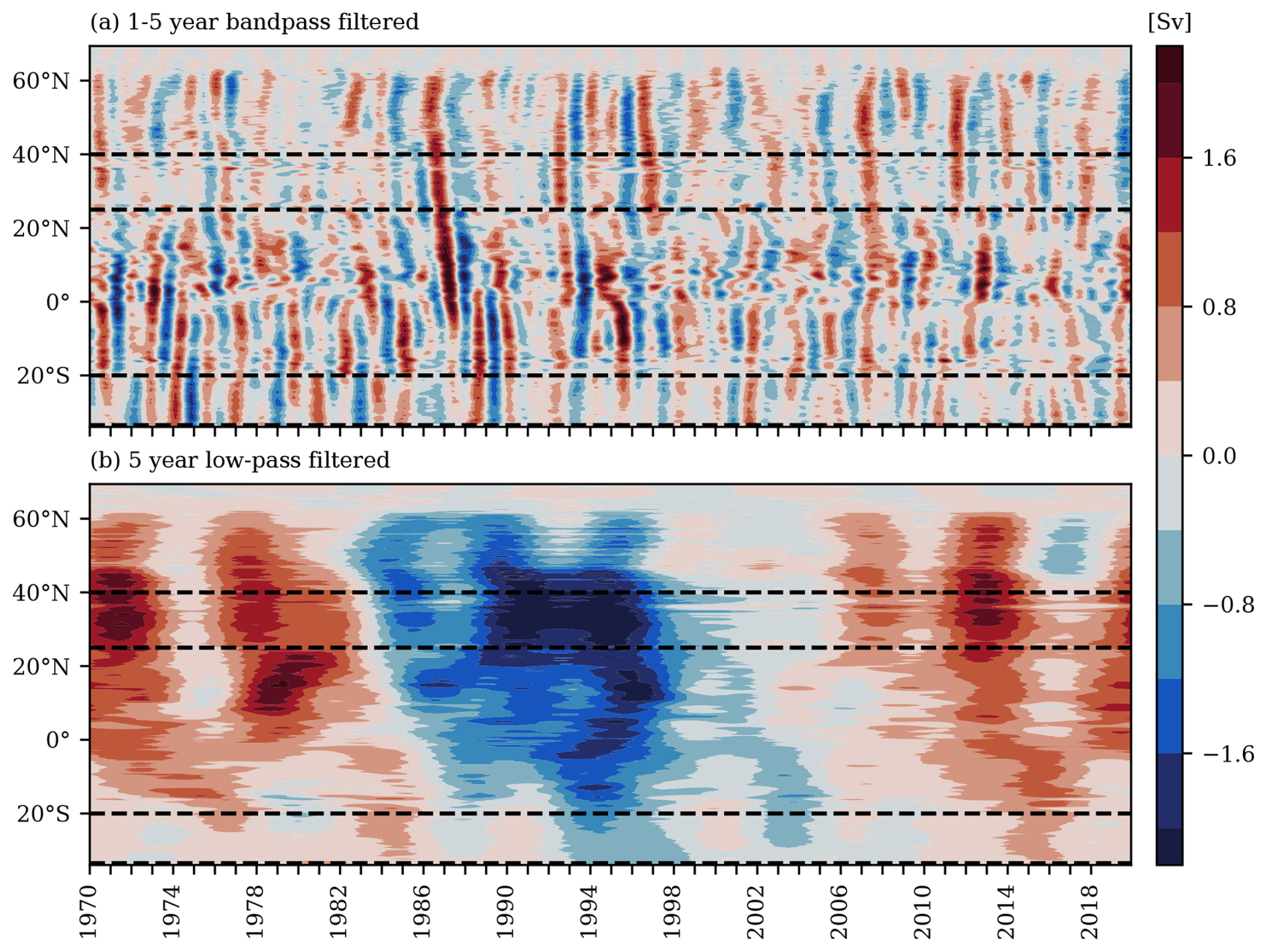
Figure 2 Hovmöller diagrams of the model-true MVT anomalies based on direct VIKING20X transports averaged over the 1000–3000 m depth range that have been filtered with (a) a 1- to 5-year band-pass filter excluding the annual cycle and (b) a 5-year low-pass filter. Horizontal dashed lines indicate the latitude interval considered in the following for both the North Atlantic (25–40° N) and South Atlantic (20–33° S).

For the 25–40° N interval, we derive a single time series of monthly MVT anomalies using the transports derived from the model streamfunction in the 1000–3000 m depth range and subtracting the mean value of 17.3 Sv (sverdrup). The results are shown in Fig. 3 based on a 5-year high-pass filtering (in panel a) and a 1- to 5-year band-pass filtering (in panel b). In the following, we will largely disregard transport variations on timescales longer than 5 years, as satellite missions operating in a low Earth orbit of approximately 500 km usually have a nominal mission lifetime of only 5 years due to atmospheric drag effects. Therefore, inferring variations over longer periods requires connecting measurements from more than one satellite mission, which adds additional challenges and is largely out of the scope of future mission design considerations. Thus, in the subsequent sections, we will primarily use the filtered time series of MVT variations, as shown in Fig. 3a, to investigate the connection to OBP variations along the western North Atlantic.

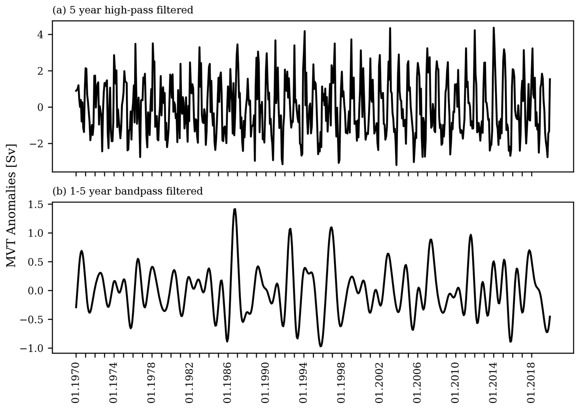
Figure 3 Time series of model-true monthly MVT anomalies in the 1000–3000 m depth range averaged between 25 and 40° N from VIKING20X. Results are shown using a 5-year high-pass filter (a) or a 1- to 5-year band-pass filter (b).

3.1 Integration approach

We now connect the filtered model MVT anomalies to OBP signals along the western continental slope of the North Atlantic. Monthly OBP fields from VIKING20X are filtered in the same way as the MVT using either a 5-year high-pass filter or a 1- to 5-year band-pass filter. Next, we calculate and plot the Pearson correlation between the model transport anomaly time series and the correspondingly filtered OBP anomalies for each grid point in the region of the western continental slope in Fig. 4. Note that we have used the negative of the transport time series here, which essentially just changes the sign of the correlations. This is done for ease of comparison with previous analyses that consider northward-directed transports.

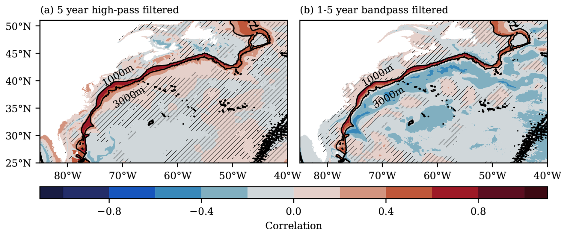
Figure 4 The Pearson correlation between model-true MVT variations in the 1000–3000 m depth range averaged between 25 and 40° N and OBP anomalies in the North Atlantic. Both MVT and OBP are either filtered using a 5-year high-pass filter (a) or a 1- to 5-year band-pass filter (b). Depth contours are indicated by dotted black lines, and regions with a p value over 0.05 are hatched. Note that we use the negative of the transport time series to be consistent with previous analyses, which usually consider northward-directed transports.

The results in Fig. 4 show a strong correlation between the model transport anomalies and OBP that is confined to the steep and narrow continental slope region between 1000 and 3000 m, matching the depth of the transport variations that we are considering here. In addition, the correlations extend farther north than the 40° N limit of the considered model transports. For both frequency bands, we find little correlation between MVT variations and OBP on the continental shelf itself. In the case of the results filtered with a 1- to 5-year band-pass filter, which additionally removes intra-annual variability, there are some modest negative correlations in the deeper ocean below 3000 m. Comparing the correlations from the two frequency bands indicates that seasonal variations are generally accessible as well, as the lower limit of the considered frequency band does not affect the correlations at the continental slope. We additionally mark regions with a low statistical significance (p value > 0.05) using hatching. This differentiation further underpins the robustness and spatial coherence of the $p_{\mathrm{W}}^{\prime }$ signals along the continental slope associated with MVT. In general, results in Fig. 4 are consistent with previous studies such as Roussenov et al. (2008), who, in contrast, assessed the northward-directed upper AMOC transports and, thus, found similar correlations.

Based on the above correlations, we can expect to be able to infer the MVT variations reasonably well from OBP anomalies along the slope. However, as we are considering the MVT between 1000 and 3000 m, based on Eq. (4), OBP anomalies at the western boundary need to be integrated vertically. Performing the integration using OBP anomalies from the western boundary, scaling with $(-f{\mathit{\rho }}_{\mathrm{0}}{)}^{-\mathrm{1}}$ and averaging over latitudes gives the time series shown in blue in Fig. 5a. Additionally, we show the direct model-based MVT anomalies in red for comparison. Note that, for visualisation purposes, we show a short time span from 1990 to 2019 only. Based on the results in Fig. 5a, we conclude that it is possible to reproduce MVT variations (a Pearson correlation of 0.76) with a root-mean-square error (RMSE) of 1.13 Sv, compared to the full transport RMS of 1.62 Sv, which results in an explained variance of 0.51.

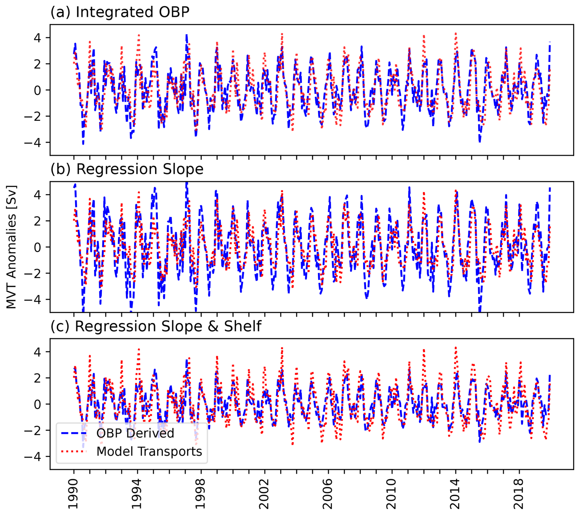
Figure 5 MVT anomalies inferred through OBP anomalies from the western North Atlantic averaged between 25 and 40° N (blue). Panel (a) uses vertically integrated OBP anomalies along the continental slope. Panel (b) considers the spatially averaged OBP anomalies from the slope region with a regression-based scaling factor. Panel (c) uses the average OBP anomalies from the western continental slope and the shelf region with two regression-based scaling factors to best represent transport variations. Model-true transport anomalies are given in red. All time series are filtered with a 5-year high-pass filter.

3.2 Regression approach

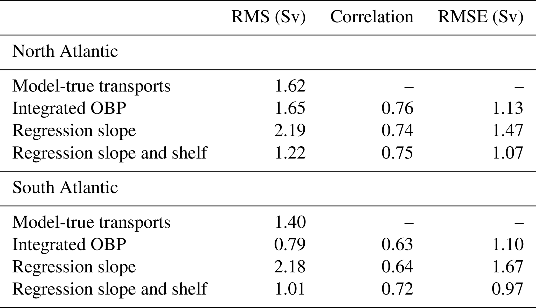
Putting the analyses of the previous section into the context of satellite gravity measurements, however, a numerical integration as performed above based on Eq. (4) will not be feasible, as the smallest spatial scales are dominated by correlated errors. Even for future constellations that will consist of multiple satellite pairs such as MAGIC, the required spatial resolution is beyond reach. Instead, satellite measurements could possibly yield the average mass anomalies over the slope region. The previous studies of Pail et al. (2015) and Daras et al. (2024) have assessed the capabilities of future double-pair satellite gravimetry missions to recover narrow OBP signals in relation to spherical harmonic truncation and noise, indicating that a double-pair mission could provide useful information up to degree and order 60–85. Although this degree of expansion allows for the partial recovery of the slope OBP signals, spatial variations are not accessible. Hence, deriving MVT anomalies will likely require a scaling procedure. One option might be to use model simulations to derive such a scaling relationship. To test the efficacy of such an approach, we average OBP anomalies in the slope region between 25 and 40° N, giving a single time series of OBP anomalies. Next, we fit a single scaling factor such that the OBP time series best reproduces the model MVT anomalies in terms of a simple linear regression. The resulting time series is given in Fig. 5b. The scaling factor derived in this case is −0.24 Sv Pa⁻¹. Using this approach reduces the correlation between scaled OBP anomalies and transport variations only slightly to 0.74 and increases the RMSE by 0.34 Sv, as shown in Table 1. Reconstructing MVT using the average OBP is, thus, still possible but adds some further complication in terms of additional noise and the required scaling factor.

Table 1 Summary statistics for comparisons of modelled and OBP-based MVT anomalies. Tabulated are the RMS values for each time series, along with the Pearson correlation RMSE values between the model transport anomalies and OBP-inferred transports using the integrated OBP based on Eq. (4), the average OBP from the continental slope through a regression, or a regression employing both the slope and shelf OBP. Both the North and South Atlantic are considered.

So far, the analyses have focused exclusively on OBP signals along the continental slope. In principle, this has the advantage that background signal levels are smaller compared to the adjacent deep and continental shelf regions; thus, a larger fraction of variability is related to changes in MVT. The disadvantage is that we focus on a target area with very limited cross-slope extent. As an alternative, signals on the continental shelf offer the possibility to improve the estimation of transport variability, as the OBP variations on the shelf partly reflect the upper northward limb of the upper AMOC cell. As upper and lower limbs should generally compensate for each other on the considered timescales and, hence, share the same variations, adding information from the upper branch might improve our estimate.

Therefore, we modify the regression approach by considering the OBP signals on the continental shelf and the signals at the slope. We do this by calculating averages over the two regions (0–1000 and 1000–3000 m depth between 25 and 40° N), multiplying each by its associated scaling factor and calculating the difference between the two. We use the difference because the OBP signals on the shelf are related to transport variations in the opposite direction. The two scaling factors are determined again through a single regression to best fit the MVT anomalies. The resulting scale factors in this case are $s_{\mathrm{slope}}=-\mathrm{0.13}$ Sv Pa⁻¹ and $s_{\mathrm{shelf}}=\mathrm{4.2}\times {\mathrm{10}}^{-\mathrm{3}}$ Sv Pa⁻¹. The difference in scale between the two does not necessarily mean that there is little weight from the shelf region, as the variability on the continental shelf is of higher amplitude (see Fig. 1). Additionally, because we determine both factors in a single regression, s_slope here deviates from the result in the previous section. We note that the scale factor for the shelf region is rather close to the value of $-\mathrm{5.9}\times {\mathrm{10}}^{-\mathrm{3}}$ Sv Pa⁻¹ found for the shelf by Bingham and Hughes (2009), who considered the upper part of the overturning cell (hence the difference in sign). The differences between the magnitudes of the two values could be explained by the larger amplitude of coastal sea level compared to averaged OBP anomalies. Based on the new scale factors, the inferred upper MVT anomalies are calculated as follows:

$$\begin{array}{}\text{(5)}& T_{\mathrm{OBP}}^{\prime }={\stackrel{\mathrm{‾}}{p}}_{\mathrm{slope}}^{\prime }\cdot s_{\mathrm{slope}}-{\stackrel{\mathrm{‾}}{p}}_{\mathrm{shelf}}^{\prime }\cdot s_{\mathrm{shelf}},\end{array}$$

and they are shown in Fig. 5c. Including the contribution from the shelf region increases the correlation with the model-based MVT time series by 0.01 (to 0.75), whereas the RMSE between the two quantities drops to 1.07 Sv (see Table 1) and the RMS of the transport estimate is reduced to 1.22 Sv. While the additional inclusion of OBP from the shelf region increases the amount of noise, this method has the advantage that the component of the OBP signal that is common to the shelf and slope is partly removed. This is similar to the removal of the depth-average as suggested by Bingham and Hughes (2008), although likely not as effective.

The suitability of this approach for application in satellite gravimetry remains to be tested. While it increases the spatial extent of the mass variations, it comes at the cost of a much higher noise level on the shelf (i.e. OBP signals that are unrelated to changes in MVT). In addition, the target region borders landmasses and, thus, potentially increases adverse impacts of hydrological signal leakage and temporal aliasing – two well-known weaknesses of satellite gravimetry. As a compromise, one could still use the shelf signals but exclude the shallowest waters. Thus, investigating which approach and regional constraint is best suited for satellite applications remains to be explored in end-to-end satellite simulation studies.

3.3 Deep-ocean OBP signals

While the analyses of the previous sections indicate that satellite-based OBP measurements may allow variations in MVT to be monitored, Landerer et al. (2015) presented an analysis based on monthly JPL-GRACE mascon solutions that specifically targeted the transport of LNADW. Focusing on depths between 3000 and 5000 m at 26.5° N, the authors reported good correlation with RAPID-based transports, especially for the anomalously weak MVT during the boreal winter of 2009–2010. However, these results are not uncontested (Hughes et al., 2018), particularly given the effective resolution of the JPL-GRACE mascons (3°). Model-based analyses conducted over longer time periods (Fig. 4, Roussenov et al., 2008; Hughes et al., 2018) show a rather strict confinement of transport-related OBP signals to the continental slope region with overall smaller amplitudes than those analysed by Landerer et al. (2015).

Here, we test whether some of the identified correlations for LNADW and OBP in the deep ocean can be reproduced using VIKING20X. First, we derive a time series of MVT anomalies for that depth range. As the results from Landerer et al. (2015) are based on 26.5° N, we average VIKING20X transports from 26° to 27° N and extract the transports between depths of 3000 and 5000 m (Fig. 6a). Next, we calculate the correlation to OBP for every grid point. The results are shown in Fig. 6 for the full resolution (panel b) and a grid with a reduced resolution of averaged 3° (panel c) to be comparable with the resolution of standard GRACE products.

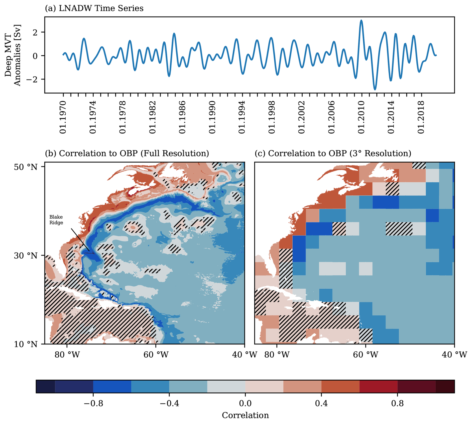
Figure 6 Time series of lower MVT anomalies (3000–5000 m depth) from VIKING20X averaged between 26 and 27° N (a). Also shown are the Pearson correlations with OBP (b, c). Panel (b) shows results using the full resolution from VIKING20X, whereas panel (c) shows the results after reducing the resolution of OBP to 3° to be roughly comparable with current GRACE data. Hatched areas show regions with a p value above 0.05. All time series are filtered using a band-pass filter to only include 1- to 5-year frequencies.

For the high-resolution case, we find the expected negative correlations along the continental slope, although at somewhat greater depths than in Fig. 4. Most pronounced are the correlations around the Blake Ridge at about 30° N. For a coarsened horizontal resolution, there are still some negative correlations around the same region, as the spatial extent is sufficiently large. For most of the rest of the continental slope or the deeper ocean, correlations are either small or patchy. Based on these results, we conclude that strongly reduced MVT transports (e.g. in winter 2009–2010), involving possible extensions of the slope signal to the wider north-western Atlantic (McCarthy et al., 2020), may indeed be observable with satellite gravimetry. However, given the expected confinement of the p_W signals to the slope region, in conjunction with the usually small magnitude of about 1 hPa for a change of 1 Sv, using standard GRACE mascon solutions seems unsuitable for reliable and regular monitoring of deep-water-transport variations. Nevertheless, it suggests that the signals that we are interested in are not totally out of reach and that data analysis approaches targeting precisely the elongated strip along the continental slope of North America are worth pursuing.

4 South Atlantic

So far, all of our analyses on the relation between OBP and MVT have been focused on the North Atlantic, in particular on the region between 25 and 40° N. In principle, however, deep-water transports at other latitudes, such as in the South Atlantic, can be inferred from boundary pressure signals as well. Thus, in this section, we focus on MVT anomalies in the South Atlantic and investigate how well they can be captured by OBP variations.

In particular, we consider the MVT between the latitudes 20 and 33° S. The southern limit of this range is determined rather ad hoc by the geographic extent of the regional refinement in the VIKING20X simulation. Previous studies indicate that the deep western boundary current breaks up into eddies at about 8° S (Dengler et al., 2004). Further south, NADW is transported by propagating eddies that affect OBP variations and could, thus, negatively impact correlations. Reaching the Vitória-Trinidade Ridge at about 20° S, the main part of the NADW flows further south as a reformed deep western boundary current (Garzoli et al., 2015; Vilela-Silva et al., 2023). As a result, we chose 20° S as the northern limit in our investigations.

Similar to the analysis performed for the North Atlantic, we first derive a single time series of MVT anomalies based on the model streamfunction by calculating the average transport between 33 and 20° S. In contrast to the previous section, however, we consider a depth range of 1100–3000 m because the transition between the northward- and southward-directed limbs is about 100 m deeper in the South Atlantic, as suggested by assessments of depth profiles (not shown here). For the same two frequency bands as before, the MVT anomalies are illustrated in Fig. 7. While the amplitude is similar to the MVT time series derived for the North Atlantic, comparing Figs. 7a and 3a indicates that the seasonal variations in VIKING20X are less dominant in the South Atlantic. As before, the time series shown in Fig. 7a for the South Atlantic region is used in the following to assess the relation to OBP anomalies.

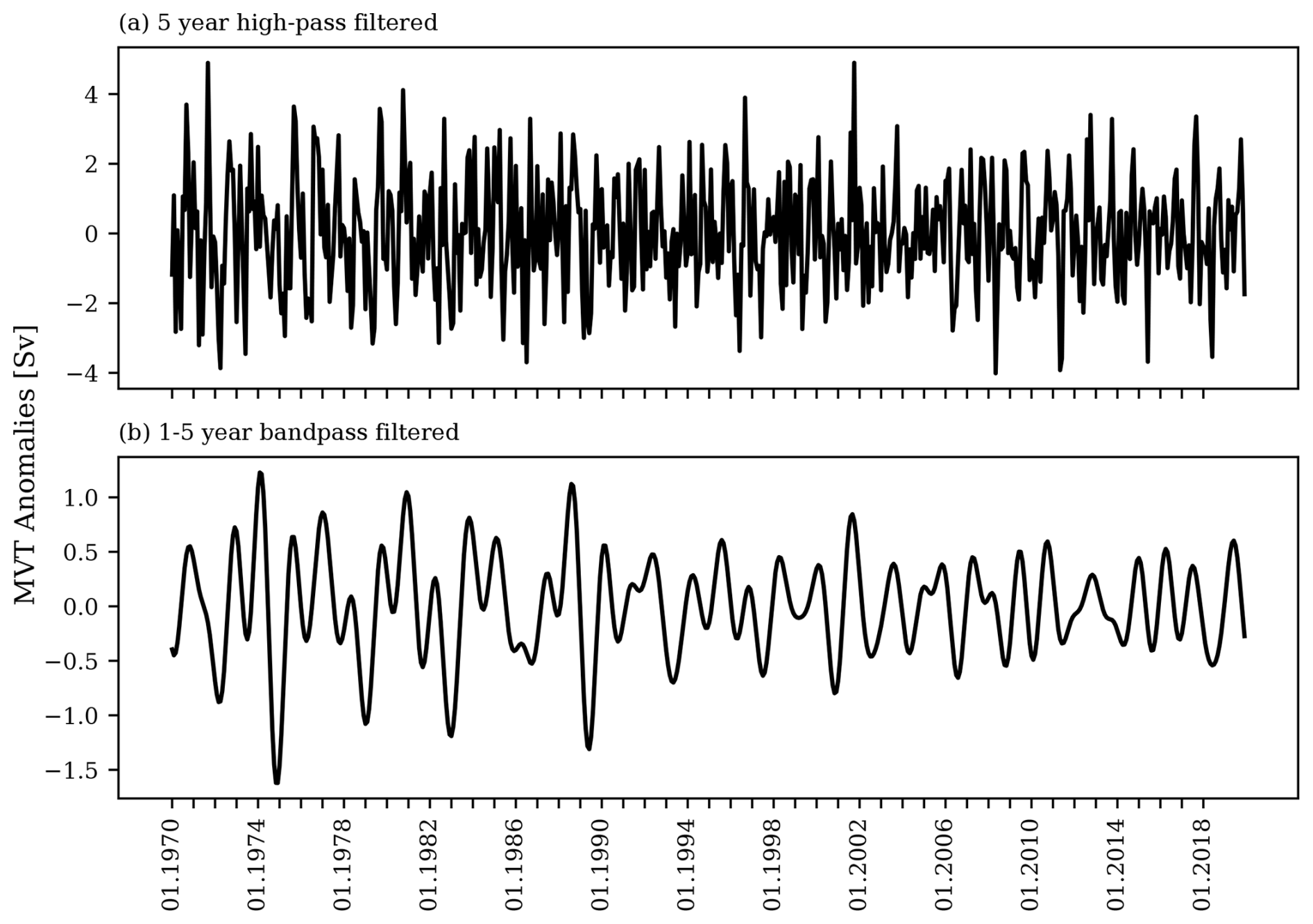
Figure 7 Time series of model-true monthly MVT anomalies in the 1100 m to 3000 m depth range averaged between 20 and 33° S from VIKING20X. Results are shown using a 5-year high-pass filter (a) or a 1- to 5-year band-pass filter (b).

4.1 Integration approach

We repeat the previous analyses, from Sect. 3.1, for the South Atlantic. As a first step, we calculate the correlation between the time series of MVT variations and OBP at the western boundary. Figure 8 shows the Pearson correlation for all grid points with either a 5-year high-pass filter (panel a) or a 1- to 5-year band-pass filter (panel b) applied. For both frequency bands, there is a moderate to strong negative correlation between the transport time series and OBP on the continental slope. Note that the correlations are negative here, as we are in the Southern Hemisphere. In this case, positive correlations are found on the continental shelf and are stronger compared to the North Atlantic. Comparing the two frequency bands, we find higher correlations using the data filtered with a 5-year high-pass filter, which suggests that seasonal signals make up a significant part of the connection between MVT anomalies and $p_{\mathrm{W}}^{\prime }$.

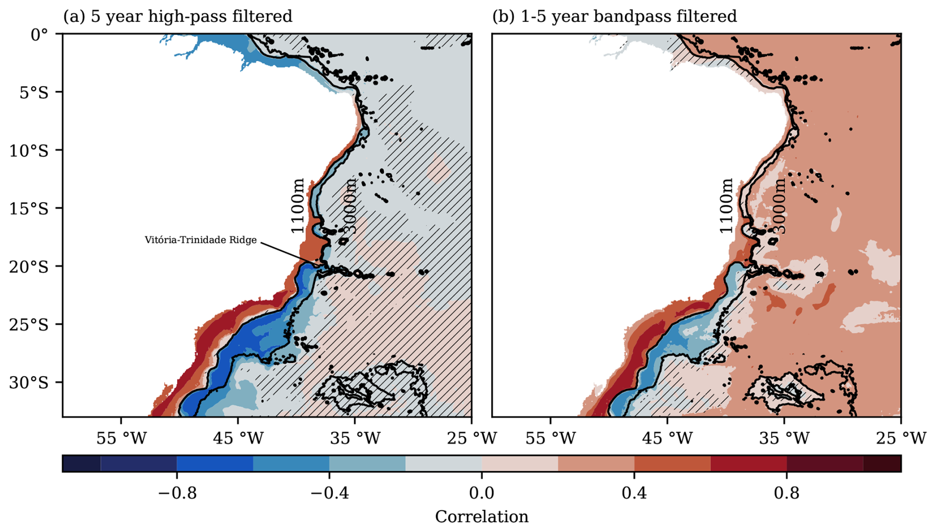
Figure 8 The Pearson correlation between model-true MVT variations in the 1100–3000 m depth range averaged between 20 and 33° S and OBP anomalies in the South Atlantic. Both MVT anomalies and OBP are filtered using either a 5-year high-pass filter (a) or a 1- to 5-year band-pass filter (b). Depth contours are indicated by dotted black lines, and regions with a p value above 0.05 are hatched.

As before, we reconstruct the MVT variations using integrated OBP anomalies on the western slope following Eq. (4). The resulting time series is shown in Fig. 9a together with the model-true MVT time series. Compared to the statistics for the North Atlantic (Table 1), the OBP-inferred time series shows a slightly weaker correlation of 0.63. The RMSE of the OBP-derived transport anomalies (1.10 Sv) is similar to the North Atlantic value, while the RMS of the model-true transport anomalies is smaller (1.40 Sv). Part of the reason for the difference in the statistics between the North and South Atlantic cases may be that the MVT transport variations have a less pronounced seasonality compared to the North Atlantic in Fig. 5a.

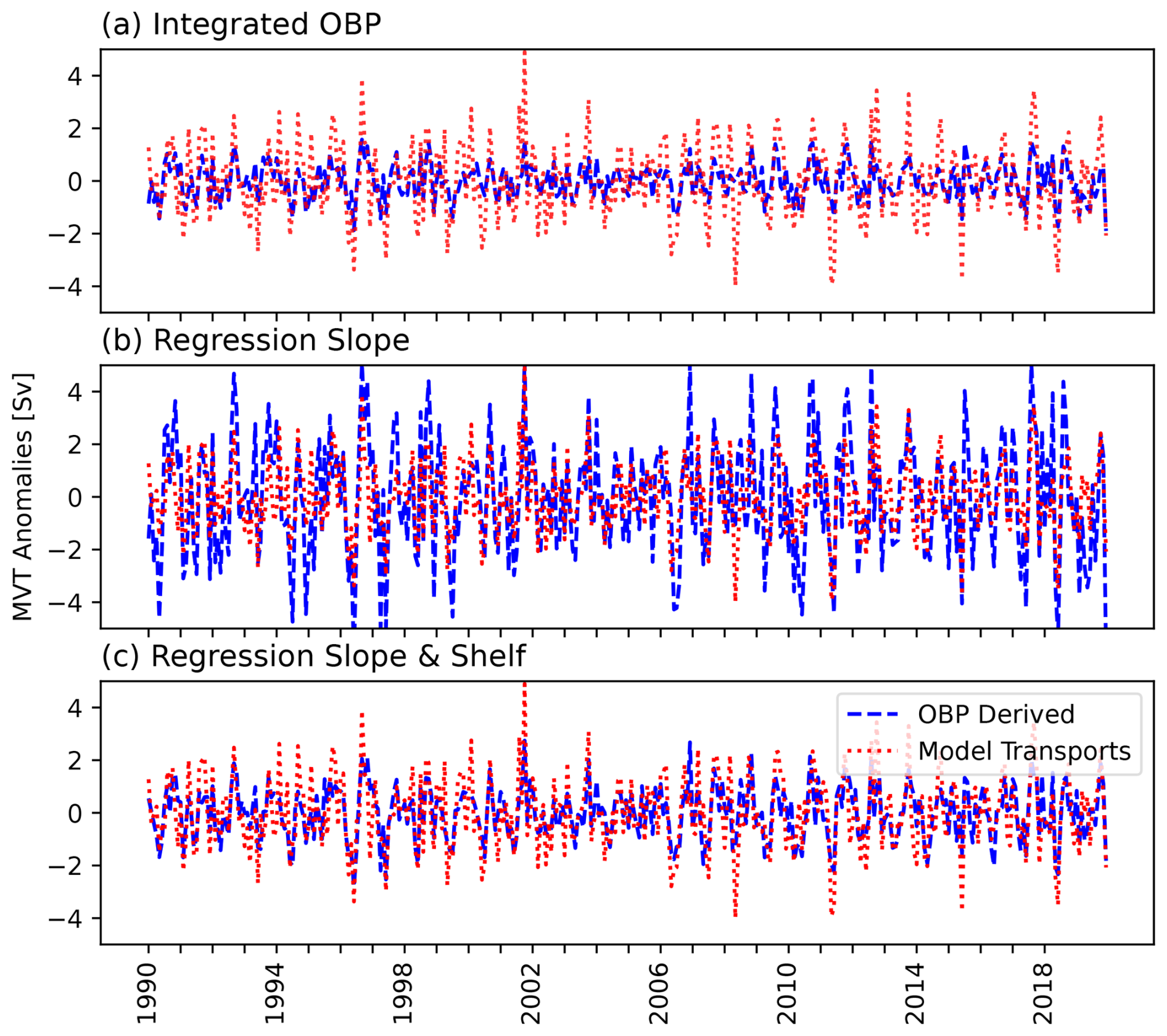
Figure 9 MVT anomalies inferred through OBP anomalies from the western South Atlantic between 33 and 20° S (blue). Panel (a) uses vertically integrated OBP anomalies along the continental slope. Panel (b) considers the spatially averaged OBP anomalies from the slope region with a regression-based scaling factor. Panel (c) uses the average OBP anomalies from the western continental slope and the shelf region with two regression-based scaling factors to best represent transport variations. Model-true transport anomalies are given in red. All time series are filtered using a 5-year high-pass filter.

4.2 Regression approach

The results of the previous section change slightly when considering the average OBP anomalies along the slope, which may be easier to sense with the means of space gravimetry. Upon averaging OBP signals and determining a scale factor to best reproduce the MVT variations (0.72 Sv Pa⁻¹ in this case), we obtain Fig. 9b. Although the correlation remains almost unchanged, the RMSE increases by 0.57 Sv, as shown in Table 1. The amplitude of the inferred MVT variations is now rather overestimated.

Lastly, we also consider the contributions from the continental shelf. As shown in Fig. 8, this region is characterised by significant correlations between the upper MVT and OBP fluctuations. Accordingly, one can expect to see some improvements in recovered transports when incorporating signals on the shelf. As described in Sect. 3.2, we do this by calculating separate averages of OBP for the continental slope and shelf regions. We then compute two scaling factors through a single regression such that the OBP-based MVT time series best reproduces the true model transport signals. In this case, the scaling factors are s_slope=0.24 Sv Pa⁻¹ and s_shelf=0.15 Sv Pa⁻¹, and they show, similar to the correlations in Fig. 8, that the shelf signal is given a significantly higher weight compared to the North Atlantic. The slope scale factor is smaller than in the North Atlantic and of opposite sign, which is to be expected based on Eq. (4) for the Southern Hemisphere. The resulting transport time series is shown in Fig. 9c. Indeed, including OBP anomalies on the continental shelf improves the correlation, as indicated in Table 1, but at the cost of introducing additional noise.

5 Synthetic time series of MVT-induced OBP variations

The analyses that we have presented so far indicate that inferring MVT transport variations through OBP anomalies along the western Atlantic is, in principle, feasible, but it requires careful consideration of the spatial extent of the region considered and the incurred noise. However, whether the variations can also be reliably tracked with future satellite gravimetry missions is not yet clear. Such tracking would involve several questions. These include the exact region to be considered as the target, the development of specific processing strategies to deal with the limited spatial resolution and possible spatial leakage, and the identification of a future mission concept that can indeed sense these OBP signals in the presence of other mass redistributions in the Earth system. Answering these points requires full end-to-end satellite simulations which offer direct control in terms of the target signal and the ability to consider adverse effects like sensor noise or aliasing artefacts in a sequential manner. To facilitate such simulations, AMOC-induced OBP anomalies need to be prepared to be compatible with existing end-to-end satellite simulation setups. In this section, we describe how such a preparation can be done based on simulated VIKING20X MVT and OBP anomalies.

The input to the simulations will be a time series of OBP anomalies for the two regions discussed above. In order to assess satellite mission concepts and develop processing strategies, it is necessary to have control over factors that complicate the signal retrieval, such as OBP signals that are unrelated to changes in MVT. We propose utilising a synthetic data set containing mostly transport-related OBP signals as opposed to the full OBP output from an ocean model. Separating the transport-related OBP signals on the slope and shelf from other OBP signals from the general circulation would allow, as a first step, for the simulation of the recovery of true transport signals and, thus, offer the simplest test case, which can then be extended by adding sources of noise.

Because the VIKING20X OBP anomalies also contain non-transport-related signals, we create a synthetic OBP time series that meets both of these requirements. We do this by performing a regression of transport variations to OBP. In essence, this is the inverse approach to the regressions presented in the previous sections. For both the North and South Atlantic regions, we take the single time series of model-true transport variations, as shown in Figs. 3 and 7a, and perform a fit to the OBP time series at each grid point determining a scaling factor for each location. Next, we multiply the regression-based scaling factor at each grid point with the model-based transport time series to create a synthetic OBP time series. The resulting data set mainly represents the OBP variations due to MVT variations at each grid point, characterised by realistic amplitudes as derived from VIKING20X. That is, the synthetic data combine the temporal behaviour of the model transports with the correct signal strength of the OBP anomalies in the model but contain no other OBP signals. Although this approach potentially includes OBP signals that correlate with – but are not dynamically linked to – transport variations, such contributions should be small and not interfere with the application of the synthetic data in satellite simulation studies.

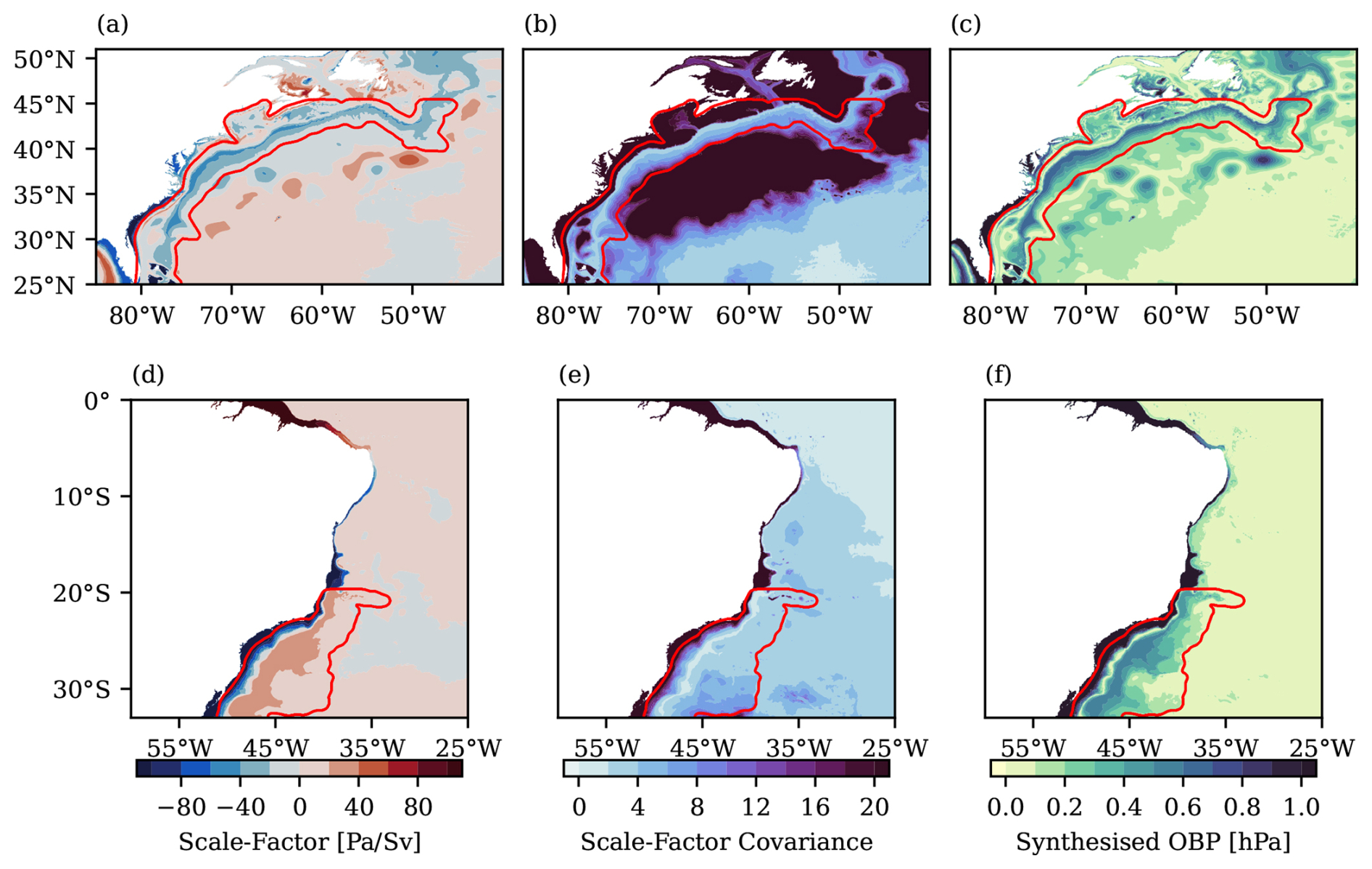
Figure 10 Results of the regression to derive a synthetic OBP time series that represents MVT variations in the North Atlantic (a, b, c) and South Atlantic (d, e, f). The scale factor from the regression of the MVT time series to OBP is given on the left, the associated uncertainty from the regression is given in the middle, and the standard deviation of the synthetic OBP time series is given on the right. All panels include a possible selection of the region of interest as a red contour.

The results of these computations for the North Atlantic are depicted in the top row of Fig. 10. The calculated scaling factor in Fig. 10a essentially reproduces the results from Fig. 4. The uncertainty in the regression is shown in Fig. 10b. Smaller values, which indicate a better fit and, thus, a more reliable result, are found mainly in the continental slope region. On the shelf and in the deeper ocean, the regression is not reliable. The standard deviation of the resulting synthetic OBP time series is given in Fig. 10c. This strip of variability along the slope is the target signal in satellite gravimetry simulation studies. In all panels in Fig. 10, we include a possible selection of the region to be supplied to simulation studies as a red outline. This region is determined by selecting the area down to depths of 4000 m, including the slope region, and applying a Gaussian smoothing to create a single coherent area. As a result, the selected region contains the continental slope as the main target as well as the signals on the continental shelf that may be of interest when considering the regression based on both regions. We base this selection on depth contours and not on the regression uncertainty, as we want to include the shelf region in the end-to-end satellite simulations because OBP on the shelf may improve the reproduction of transport variations.

Similarly, the scale factor, uncertainty and standard deviation for the South Atlantic are shown in Fig. 10d–f. Notably, the target signal for satellite gravimetry appears to be slightly wider due to the smaller gradient of the continental slope. The greater spatial extent is also reflected in the region outlined in red, in which the data are to be supplied to simulation studies. The region is determined in the same way as in the North Atlantic.

6 Conclusions

Deep-water transports can be approximated through bottom pressure anomalies at the western boundary of an ocean basin, thereby providing an opportunity to monitor these transports through satellite gravimetry missions. That said, reliable estimates from this approach will likely remain elusive with standard GRACE/GRACE-FO monthly solutions, mainly due to the limited spatial resolution of the resulting time-variable gravity fields and derived bottom pressure anomalies. However, future gravity missions, especially those consisting of multiple satellite pairs such as planned in MAGIC, may allow monitoring of MVT anomalies from space. One can expect trans-basin moorings (e.g. RAPID) to continue delivering highly accurate transport determinations, but the necessary arrays are costly and tend to be sparse, such that satellite-based observations may help to fill gaps in spatial coverage and provide continuous large-scale monitoring, provided that satellite gravimetry becomes operational.

Work toward this objective will require dedicated end-to-end simulation studies to assess the capabilities of the missions, develop processing strategies or even refine requirements for future mission scenarios. Here, we have assessed the connection between western OBP and southward-directed MVT anomalies, which, in part, reflect NADW anomalies, in the VIKING20X model for the North and South Atlantic. Correlations with OBP in the region of the western continental slope confirm previous model-based studies in that the connection is strong mainly along the slope (Bingham and Hughes, 2008; Roussenov et al., 2008; McCarthy et al., 2020). While a theoretically precise estimation of MVT variations requires a spatial integration of OBP across the slope, almost identical results can also be achieved using the average OBP anomaly from the slope region that might be accessible through satellite measurements by applying an empirically derived scaling factor. Correlations between OBP-derived and direct model transports calculated in this way are 0.74 for the North Atlantic and 0.64 for the South Atlantic. Including average signals from the continental shelf region can improve results for both the North and South Atlantic. Although the improvement in correlation for the North Atlantic is only modest (0.01), it is more significant in the South Atlantic where the correlation increases by 0.08. This would suggest that inferring MVT anomalies through OBP is not only worth investigating in the North Atlantic, as is often considered, but could also be attempted in the South Atlantic, albeit with increased levels of noise.

Based on the results using the VIKING20X data, we have also estimated a synthetic time series of OBP anomalies that can be used in satellite simulation studies. To that end, we have performed a regression of modelled MVT anomalies to OBP at each grid point. This way, the resulting synthetic OBP data include mainly the variations due to transport variations while also having realistic OBP amplitudes. In addition, we have delineated a spatial mask for the region of interest based on depth contours.

Although our results suggest that there is a connection between OBP and deep-water-transport anomalies in VIKING20X, there are additional complications that are not considered here. For one, we base our analyses on high-pass-filtered data that still include the seasonal signal. While inter-annual variations are likely of more interest, the reduced signal amplitudes make retrieval through satellite gravimetry more challenging. Thus, in order to assess the easiest test case in simulation studies, we have included the seasonal variations in our analyses. Further, we have focused on western boundary pressures, as they contain most of the transport-related OBP signals. Neglecting eastern signals introduces small errors in the transport determinations and precludes the full removal of pressure signals associated with basin-wide modes or ocean mass changes (Bingham and Hughes, 2008). In principle, a regression approach considering both the slope and shelf region can mitigate some of these OBP signals, but some impact will remain. As a result, estimates of p_W may include signals unrelated to overturning. As the synthetic OBP data to be provided for satellite simulation studies only contain overturning-related signals, this additional complication would not be captured in the simulation studies. Nonetheless, we believe that feasibility tests in satellite simulations should initially start with a clearly defined target signal, leaving the treatment of somewhat secondary aspects for later stages of refinement.

We have also not considered trend signals in MVT in view of the nominal satellite mission lifetime of just 5 years. Therefore, assessing whether trends are accessible through satellite measurements or sensitivity estimates is not possible. While this question may become more relevant in the future, estimating subtle trend signals from satellite gravimetry is generally a matter of delicacy due to superimposed signals from, e.g.  regionally variable barystatic sea level rise and glacial isostatic adjustment of the solid Earth (Chen et al., 2022).

Lastly, connecting average OBP from the western continental slope to MVT variations requires an empirically derived scaling based on the actual model transports. While such an approach is of course feasible for simulated satellite observations, deriving such a scaling suitable for actual measurements will require more careful assessments. Despite these challenges, the work presented here allows for the inclusion of transport-related OBP signals in synthetic time-variable gravity field data sets, such as the ESA Earth System Model (Dobslaw et al., 2015). This, in turn, can lay the groundwork for the thorough, albeit optimistic, assessment of future satellite gravimetry mission capabilities to monitor deep-water transports and AMOC variability and for upcoming mission performance evaluation studies for MAGIC.