Understanding uncertainties in the satellite altimeter measurement of coastal sea level: insights from a round-robin analysis

The satellite radar altimetry record of sea level has now surpassed 30 years in length. These observations have greatly improved our knowledge of the open ocean and are now an essential component of many operational marine systems and climate studies. But the use of altimetry close to the coast remains a challenge from both a technical and scientific point of view. Here, we take advantage of the recent availability of many new algorithms developed for altimetry sea level computation to quantify and analyze the uncertainties associated with the choice of algorithms when approaching the coast. To achieve this objective, we did a round-robin analysis of radar altimetry data, testing a total of 21 solutions for waveform retracking, correcting sea surface heights and finally deriving sea level variations. Uncertainties associated with each of the components used to calculate the altimeter sea surface heights are estimated by measuring the spread of sea level values obtained using the various algorithms considered in the round-robin for this component. We intercompare these uncertainty estimates and analyze how they evolve when we go from the open ocean to the coast. At regional scale, complementary analyses are performed through comparisons with independent tide gauge observations. The results show that tidal corrections and uncertainties in the mean sea surface can be significant contributors to uncertainties in sea level estimates in many coastal regions. However, improving the quality and robustness of the retracking algorithm used to derive both the range and the sea state bias correction is today the main factor to bring accurate altimetry sea level data closer to the shore than ever before.

1 Introduction

Since the early 1990s, satellite altimetry has routinely observed the ocean surface topography, resulting in a more than 30-year-long record of accurate and nearly global sea level data. These observations have greatly improved our knowledge of the open ocean and are now a key climate indicator of global warming and an essential component of many operational marine systems (International Altimetry Team, 2021).

But in coastal regions, satellite altimetry encounters different technical issues that make it difficult to derive accurate measurements of sea level within tens of kilometers from the land (for example see Vignudelli et al., 2011, for a complete review). Firstly, in the coastal band of a few kilometers width (corresponding to the altimeter footprint size, i.e., up to about 10 km depending on the satellite altimetry mission), land contamination leads to complex radar waveforms that are difficult to interpret in terms of geophysical parameters through the common process called retracking (Deng and Featherstone, 2006; Gommenginger et al., 2011). The other main limitation is related to the geophysical and environmental corrections that need to be applied to the altimeter measurements to compute the height of the ocean surface (e.g., wet troposphere, ionosphere, sea state bias, inverse barometer, high-frequency wind effect and tides) and that often become inaccurate close to the coast (e.g., Vignudelli et al., 2005; Andersen and Scharroo, 2011). Finally, the traditional use of sea level anomalies (SLAs) in oceanography applications requires the removal of a time average of the height of the ocean surface, called the mean sea surface height (MSSH). In near-shore areas, the MSSH is contaminated by the same suite of retracking and correction errors as those that arise in the process of computing the height of the ocean surface (Andersen and Scharroo, 2011; Gómez-Enri et al., 2019).

Filling the altimetry data gap in the coastal zone is needed to explain, estimate, and plan for coastal impacts associated with sea level changes induced by ongoing global warming and has motivated a number of coastal altimetry studies, inducing significant progress during the last decade (Cipollini et al., 2017; Birol et al., 2021). In order to address the limitations mentioned above, new retracking algorithms have been developed to reduce the contamination of spurious signal components in the coastal zone (Passaro et al., 2014; Peng et al., 2018; Thibaut et al., 2021). In parallel, significant improvements have also been achieved in altimeter corrections (e.g., wet-tropospheric and ocean tide corrections, sea state bias), allowing more accurate altimetry-derived coastal sea level data to be obtained (Fernandes et al., 2015; Lyard et al., 2021; Passaro et al., 2018). New MSSH products are also available (Sandwell et al., 2017; Schaeffer et al., 2023). These efforts improve the performance of altimetry in the coastal ocean with respect to the standard solutions provided by space agencies and operational altimetry services. Some of the new algorithms developed are progressively introduced in the operational processing baselines. However, the metrics used to measure the performance improvement and the coastal area generally change from one study to the other, making it difficult to provide an objective comparison of their relative merits.

Today, several algorithms are available for calculating the range, for most of the geophysical corrections and for the MSSH used to derive coastal SLAs from altimetry measurements. The main objective of this paper is to take advantage of them to better understand the sources of uncertainties linked to the processing algorithms in the sea level computation when approaching the coast. Particular attention is also paid to the transition between the open ocean and coastal ocean. To this end, a round-robin exercise has been done for the components of the altimetric SLAs for which several solutions existed. In each case, as many algorithms as possible were tested with similar metrics to have a common analysis methodology. For each component, we can then objectively discuss the relative performance of the different algorithms in terms of the selected diagnostics. But, assuming that the differences between algorithms reflect the associated uncertainties, we can also analyze and compare how these uncertainties are then reflected in the calculation of the SLA data as we get closer to the coast.

This paper is organized as follows: the objectives and the data used in the round-robin analysis are described in Sect. 2. The methodology is presented in Sect. 3. Results and discussions for each of the sea level components evaluated are provided in Sect. 4. Section 5 summarizes the main results and gives some perspectives.

2 Objectives and input data of the round-robin analysis

2.1 General goals

Altimetry technologies have considerably evolved in recent years with the delay-Doppler mode (or SAR for synthetic aperture radar) and the SAR interferometric (SARIn) mode. Here, we have chosen to focus on the conventional low-resolution mode (LRM) technique only because it has the largest time span and number of altimetry missions, with seamless continuity from the first generation of climate reference altimeters (in the 1990s) until today. For this reason, it also provides the largest number of algorithms available to derive geophysical parameters from corresponding altimetry measurements, including some specific developments to improve the data quality near the coast (Fernandes et al., 2015; Passaro et al., 2014). Note then that the results presented below are specific to LRM altimetry data.

The round-robin exercise presented in this study was implemented to intercompare algorithms used to calculate the SLAs from LRM altimetry measurements in order to evaluate their accuracy. In what follows, we will not go into the technical details of the radar altimetry techniques, as it is thoroughly explained elsewhere (e.g., Fu and Cazenave, 2001). In summary, satellite altimetry is based on a radar altimeter sending/receiving pulses/echoes towards/from the overflown surface. By analyzing the backscattered echoes (the so-called waveform), we can deduce the altimeter range (i.e., the distance between the satellite's center of mass and the mean reflected surface) through a process called retracking. The transformation from the range into SLAs then requires knowledge of auxiliary information (e.g., satellite altitude, atmospheric and geophysical corrections, MSSH). Finally, the SLA is computed according to Eq. (1):

$$\begin{array}{}\text{(1)}& \begin{array}{rl}\text{SLA}& =\text{altitude of satellite}-\text{altimeter range}\\ & -\text{ionospheric correction}\\ & -\text{dry tropospheric correction}\\ & -\text{wet-tropospheric correction}\\ & -\text{sea state bias correction}\\ & -\text{solid earth tide correction}\\ & -\text{geocentric ocean tide correction}\\ & -\text{geocentric pole tide correction}\\ & -\text{dynamic atmospheric correction}\\ & -\text{mean sea surface height}\end{array}\end{array}$$

Each of the terms of Eq. (1) will be called “SLA component” hereinafter. Any systematic error in any of these terms directly results in errors in the SLA estimates. The SLA components are all derived from numerical or empirical models or from altimetry or auxiliary observations. For most of them, different solutions exist. When available, we have included solutions developed specifically for the coastal environment (see Sect. 2.2). The algorithms are then intercompared with common metrics (see Sect. 2.3).

This study focuses on altimetry data of the coastal zone, whose definition varies widely from one study to the other (Laignel et al., 2023). Here, to take a broad reference, we define the global coastal zone as the geographical area between the coastline and 200 km offshore, at global scale (Fig. 1). Because they provide SLA data closer to the coast (Birol et al., 2021), we consider along-track altimetry measurements at the original high-frequency sampling rate (20 Hz).

Coastal conditions being different from one region to the other, the uncertainty sources in altimetry sea level may have a marked geographical dependency. It was consequently decided to carry out this study at both global and regional levels. For this purpose, three coastal areas were chosen because of their very different coastal and oceanographic contexts and because of the availability of regional ocean tide corrections (Sect. 2.2): the Mediterranean Sea, the northeast Atlantic Ocean and eastern Australia (Fig. 1).

Moreover, in order to estimate the degree of agreement of our results from one altimeter to another, we consider data from the two reference missions Jason-2 and Jason-3 as they flew on the same nominal orbit (see below).

Finally, note that the focus of this round-robin study is the comparison of different processing solutions in order to gain insight into the associated sources of uncertainties in sea level data when approaching the shoreline. Even though we compare the algorithms against each other with a set of performance assessment criteria, we do not aim to identify here the “best” algorithm among all those tested to compute SLAs. The ranking of algorithms depends mainly on user needs, which in turn define the best set of metrics to use in that particular case. The final choice for a given application can then only be a trade-off between different criteria (e.g., computational cost, availability of the algorithm/solution, continuity between altimetry missions, improvement of long scales over white noise).

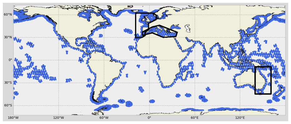
Figure 1 In blue, geographical domains and segments of altimetry tracks (blue dots) considered in the round-robin study. The northeast Atlantic, eastern Australia and the Mediterranean Sea used in the regional analyses are indicated by black squares. All of them comprise the [0–200] km coastal band except the Mediterranean Sea, which is complete; the Black Sea is excluded.

2.2 Overview of the selected algorithms

To achieve the objectives of this study, it was crucial to have access to as many algorithms as possible, including those used in the operational sea level products (i.e., the level 2 Geophysical Data Record or GDR products; see https://www.aviso.altimetry.fr, last access: 8 November 2024). To collate all the data, we used the CNES (French Space Agency) internal altimetry database that contains all the operational Jason-2 and Jason-3 GDR products (CNES, 2024), where we could add project-oriented datasets that were made available for the purpose of this study (e.g., outputs of the ALES and Adaptive retrackers, regional tide solutions; see Table 1 for complete information). For an objective evaluation of the results from the metrics computed for both Jason-2 and Jason-3, we have selected 3 years of data (i.e., 111 cycles) for each of these altimetry missions. For Jason-2, cycle 193 (start: 27 September 2013) to cycle 303 (end: 2 December 2016) have been chosen. For Jason-3, the dataset covers cycle 1 (start: 17 February 2016) to cycle 111 (end: 22 February 2019).

Concerning the SLA components of Eq. (1), the altitude of satellite, dry tropospheric correction and the dynamic atmospheric correction were not be included in the round-robin because only one solution was available for each of them. The solid earth tide height and the geocentric pole tide height were also discarded because they are considered very accurate and non-critical for coastal sea level calculations (Andersen and Scharroo, 2011). For the other components, the main criterion to select the algorithms was the availability of the corresponding dataset at global scale and for the whole study time period (i.e., 27 September 2013 to 22 February 2019). A few exceptions have been made for specific reasons explained below.

The altimeter range and the sea state bias correction (SSB) derived from the ALES retracker (Passaro et al., 2014) are part of the ESA Climate Change Initiative (CCI) Coastal Sea Level product (Cazenave et al., 2022). These datasets are not global but cover a large part of the coastal ocean (except latitudes above 60° N; Japan, Alaska, and the Okhotsk Sea and Bering Sea zones in the north; and New Zealand, Antarctica and some small islands in the south, as shown in Fig. 1 of Cazenave et al., 2022). Because the ALES retracker has been shown to improve coastal altimetry sea level retrieval in comparison with the standard MLE4 (maximum likelihood estimator) retracking algorithms (Passaro et al., 2015), this study would not be complete without its inclusion. As a consequence, all the algorithms concerning the altimeter range and the SSB will be evaluated only where ALES data are available.

The geocentric ocean tide is one of the main contributors to the sea level variations in regions with strong tidal motions, which is the case of a large part of the global ocean continental shelves. Tides must be removed from satellite altimetry data using hydrodynamic models in order to avoid aliasing issues with other ocean dynamic signals (Chelton et al., 2001). Even if tidal modeling benefited from many improvements these last years, the most recent global models still show errors of several centimeters in coastal regions (Stammer et al., 2014; Lyard et al., 2021). The development of regional models at higher resolution improves the estimation of ocean tides on the continental shelves and consequently provides more accurate altimetry corrections (Cancet et al., 2018). Including such regional tidal models in this study allows us to analyze the uncertainties associated with the use of global tidal models in computing altimetry coastal sea level. The ocean tide correction from the regional tidal model is, by definition, available only in its geographical area. For this project, regional tidal corrections were made available by CNES–NOVELTIS for the Mediterranean Sea, the northeast Atlantic and eastern Australia regions. The evaluation of all the algorithms concerning the ocean tide correction will then be done only at regional scale. For comparisons at global scale, readers can for example refer to Stammer et al. (2014) and Lyard et al. (2021).

Concerning the SSB, some of the most recent datasets (i.e., MLE4 2D 20 Hz, MLE4 3D 20 Hz, Adaptive 3D 20 Hz) currently exist as prototypes only for Jason-3 and not for Jason-2. Given that the SSB is identified as a large source of uncertainty in altimetry sea level retrieval, particularly 10–15 km from the coast (Andersen and Scharroo, 2011; Passaro et al., 2018), it was decided to include these algorithms in this study. As a consequence, the metrics concerning the SSB will be computed only for Jason-3.

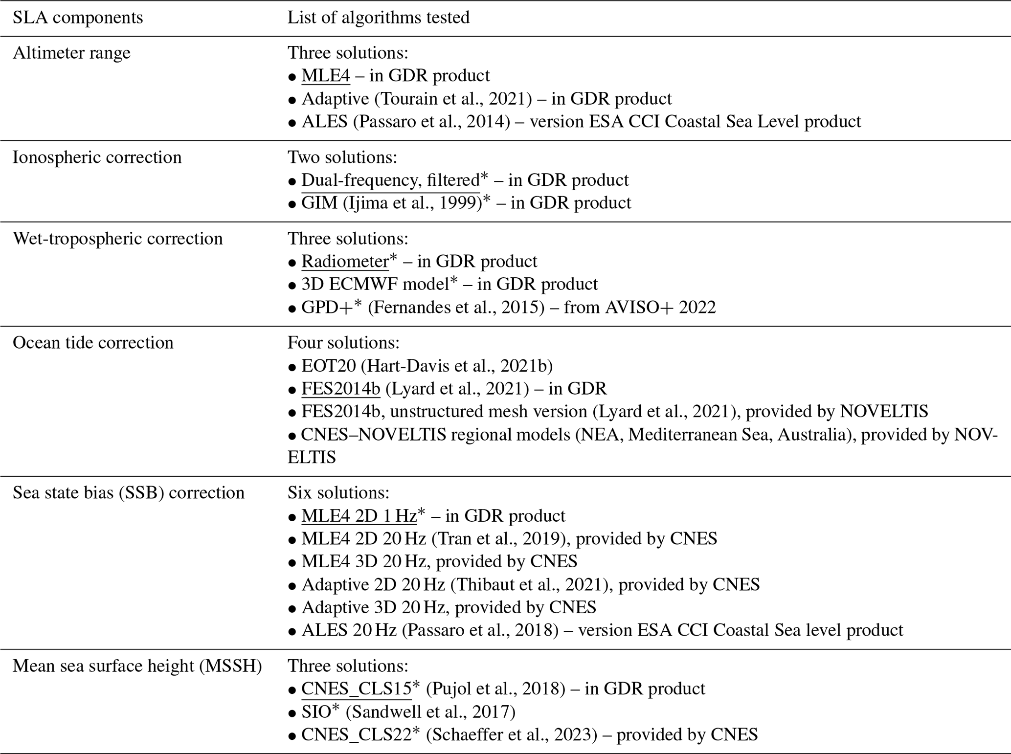
Finally, the SLA components and algorithms used in this round-robin are listed in Table 1. They represent a total of 6 components and 21 algorithms.

Table 1 SLA components included in the round-robin exercise (column 1), with the list of algorithms tested for each one (column 2). The reference algorithms currently used in operational sea level products for each component are underlined. The fields marked with an asterisk (^*) were provided at 1 Hz only and have been linearly interpolated to 20 Hz for the purposes of this study; the others were at 20 Hz. GDR is the official Geophysical Data Record product distributed by the space agencies (version D for Jason-2 and version F for Jason-3).

2.3 Tide gauge data

At regional scale, some of the metrics used to estimate the accuracy of altimetry coastal sea level derived with the different algorithms listed in Table 1 are based on comparisons with independent hourly sea level observations from tide gauges. Tide gauge measurements from the following databases have been used:

• Mediterranean Sea – CMEMS (https://marine.copernicus.eu, last access: 15 October 2021), Refmar (http://refmar.shom.fr/, last access: 15 October 2021) and ISPRA (https://www.mareografico.it/, last access: 15 October 2021);

• northeast Atlantic Ocean – BODC (https://www.bodc.ac.uk/, last access: 15 October 2021), Refmar (http://refmar.shom.fr/en/home, last access: 15 October 2021) and UHSLC (https://uhslc.soest.hawaii.edu/, last access: 15 October 2021);

• eastern Australia region – UHSLC (https://uhslc.soest.hawaii.edu/, last access: 15 October 2021) and BOM (http://www.bom.gov.au/, last access: 15 October 2021).

For all these databases, the tide gauge stations selected for this study had to meet the following selection criteria (all of them must apply):

• quality data available over the whole study period (2013–2019, but time series with many data gaps longer than 5 d were not considered)

• stations located at a distance shorter than 50 km from a Jason-2 or Jason-3 nominal track, avoiding locations sheltered by islands or inside estuaries, so that the ocean dynamic signals captured by the in situ instrument and the satellite altimeter are as similar as possible.

From all the considered databases, 13 stations met these criteria in the northeast Atlantic region, 12 in the Mediterranean Sea and 8 in the eastern Australia region (see Fig. 2).

To compare the altimetry and tide gauge sea level measurements, the tidal signal has been removed from the tide gauge sea level time series using a harmonic analysis approach. The effect of atmospheric pressure and wind on the tide gauge sea level has been removed using the same correction as for the altimetry observations (dynamic atmospheric correction from MOG2D solution; LEGOS/CNRS/CLS, 1992; Carrère and Lyard, 2003).

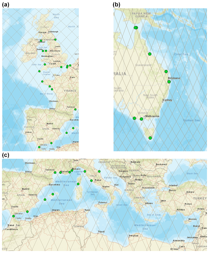
Figure 2 Jason-2 and Jason-3 nominal tracks (dashed black lines) and tide gauge stations (green dots) used in this round-robin study in the northeast Atlantic (a), eastern Australia (b) and Mediterranean Sea (c).

3 Methodology

The basic principle of this round-robin study is to compare all the selected SLA components and algorithms using the same metrics so that their impact on the coastal sea level computation can be assessed in the same way. In order to measure the consistency of all the results between different altimetry missions, the same analysis has been done for both Jason-2 and Jason-3 (with the exception of the SSB component; see Sect. 2.2) at global and regional scales (i.e., in the three regional domains shown in Figs. 1 and 2). For each SLA component, the accuracy is investigated by analyzing the dispersion of SLA values we obtain using the various corresponding algorithms mentioned in Table 1, with a focus on the coastal ocean. At regional scale, the analysis is completed with a comparison to independent tide gauge observations.

In practice, the study has been organized by SLA component. At global scale, for each of them, the different algorithms have been first intercompared in terms of data availability (spatial pattern of the data availability, data availability as a function of distance to the coast) and general statistics (mean, standard deviation, histograms of values). Then, the impact on the SLA calculation has been analyzed for each algorithm tested for this component. Therefore, only one term (algorithm) of the SLA definition (Eq. 1) changes at a time. All the other SLA components are the state of the art of the operational sea level products at the time this study was conducted (see algorithms that are underlined in Table 1). They are considered here as the reference algorithms. At regional scale, the intercomparison between the different algorithms has been done not only in terms of data availability and general statistics, but also in terms of comparison to the tide gauge measurements (statistics and local altimetry data availability).

Before carrying out statistical analyses, because original altimetry measurements are not sampled exactly at the same points at each cycle, all the along-track sea level components and SLA values were binned along average ground tracks of the Jason missions with a resolution of 20 Hz (i.e., ∼ 0.3 km). When computing metrics on the SLA components, no editing was applied and all values available in the dataset were used. For the metrics on the SLA itself, values outside the window [−3 m; 3 m] were systematically discarded everywhere. In the Mediterranean Sea, associated with generally lower SLA variations, a stricter window [−1 m; 1 m] was applied. For each SLA point time series, outliers outside a 4σ window have also been removed from the computations, σ being the standard deviation of the SLA time series. Finally, altimetry points have been binned considering their distance to the coast (Figs. 3, 5, 6, 9, 10, 11). To ensure robust global or regional statistics, we considered a fixed number of altimetry points in each bin, with the bin size varying from about 300 m at the coast to 1.2 km at 200 km from the coast, as the distribution of altimetry points as a function of the distance to the coast shows a higher density of points close to the coasts due to the presence of islands and to the tracks' configuration.

Concerning the comparison between altimetry and in situ SLAs, for each tide gauge station, the nearest satellite track to the station is selected. Only altimetry data located at a distance to the coast shorter than 20 km and at a distance to the tide gauge station shorter than 40 km are used.

In the end, we have evaluated 21 algorithms at global scale and for the three study regions for both the Jason-2 and Jason-3 missions (when possible). The total number of intercomparison diagnostics reaches several hundred. As it represents a considerable amount of work that can be useful for purposes other than those of our study, they all have been made available at https://www.aviso.altimetry.fr/en/data/ (last access: 8 November 2024) so that colleagues can use them for other applications. In the following section, we will only show some of the results obtained in line with the objectives of this study.

4 Results

4.1 Ionospheric correction

The commonly used method to compute and correct the altimeter range for the delay effects due to the ionosphere is the linear combination of data measured at two different radar frequencies (Chelton et al., 2001). The corresponding dual-frequency correction is considered less accurate in coastal areas due to altimeter echoes and a required along-track filtering (Fernandes et al., 2014), and both can be altered by land contamination in these areas. A second method consists of using external models, and the GNSS-based global ionospheric maps (GIMs; Komjathy and Born, 1999) are the most commonly used corrections for single-frequency altimeters and for coastal and inland applications (Dettmering and Schwatke, 2022). In the following, we estimate the relative uncertainties of these two solutions for the ionospheric correction as they approach the coast by comparing their respective statistics.

Here, only the example of Jason-2 is presented. Figure 3 shows the global mean of the standard deviation (SD) of the SLA computed with each of the two corrections (top and middle panels a and b) and the spread of the differences in these SDs of SLAs (bottom panel c), as a function of the distance from the coast. Note that the increase in the SD values below 10 km from the coast (Fig. 3b, middle) is generally observed in this type of diagnostic and is largely related to an increase in the SLA errors near the coastlines (Andersen and Scharroo, 2011). It integrates the errors in all the different SLA components and does not necessarily reflect firstly those of the ionospheric correction. However, between the two solutions, we observe a difference of 0.1 cm in SD beyond 20 km from the coast, which then increases up to ∼ 0.75 cm in the last 5 km.

The standard deviation of the differences obtained between the SLA solutions (Fig. 3c) also clearly increases when approaching the coast. The corresponding spread values remain below 0.2 cm in the open ocean up to 40 km from the coast, then range between 0.2 and 0.7 cm between 10 and 40 km, and finally increase up to 2.8 cm in the last 10 km. These numbers can be considered an estimate of the SLA uncertainty due to the ionospheric correction.

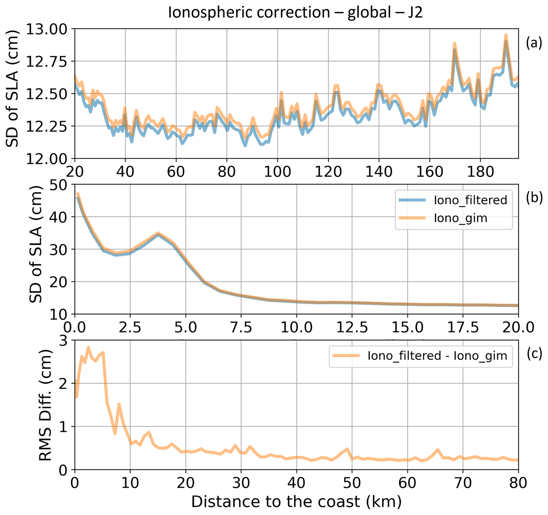
Figure 3 (a, b) Global mean of standard deviation values (in cm) of the SLA along all Jason-2 tracks for the period 27 September 2013 to 2 December 2016 when applying different ionospheric corrections (dual-frequency filtered in blue, GIM in orange). Results are represented as a function of the distance to the coast (in km) between 200 and 20 km (a) and between 20 and 0 km from the coast (b). (c) Global standard deviation of the differences in standard deviation values (in cm) of the SLA when applying the different ionospheric corrections between 80 and 0 km from the coast.

Figure 4 illustrates that this average result at global scale presents some geographical features, with lower/larger SLA SD values generally obtained with the dual-frequency solution below/over 15–20° N/S. These latitudinal patterns are very consistent with the large-scale features of the mean and variability of the ionospheric corrections (Fernandes et al., 2014). When analyzing the tide gauge comparison statistics, no significant differences were found between the two SLA datasets (not shown here, but see the reports under the link provided at the end of Sect. 3). This could be due to the fact that the regions considered in our study show small differences between the ionospheric solutions (see northeast Atlantic (NEA), Mediterranean Sea and eastern Australia in Fig. 4), as the associated uncertainties in SLA potentially do.

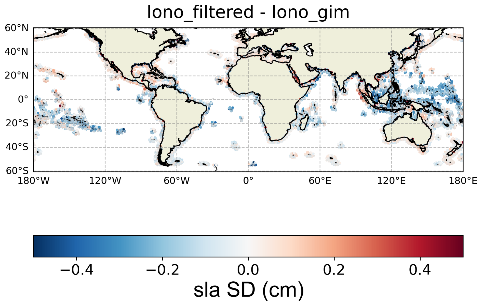
Figure 4 Map of the differences in standard deviation of the SLA (in cm) along all Jason-2 tracks for the period 27 September 2013 to 2 December 2016 when applying the dual-frequency ionospheric correction compared to when using the GIM model. Results are only shown between 200 and 0 km from the coast.

4.2 Wet-tropospheric correction

The wet-tropospheric correction (WTC) is related to the path delay in the altimeter return signal due to cloud liquid water and water vapor in the atmosphere. It can be derived either from meteorological models or from a microwave radiometer on board the altimetry mission. Due to the large space–time variability in this correction (0–50 cm), the latter is generally considered the best option over the ocean (Obligis et al., 2011). Lázaro et al. (2020) report an associated reduction of 1.2–2.2 cm² in the SLA variance on average between 0 and 200 km from the coast. However, because of the radiometer footprint, this WTC is known to decrease in quality starting at ∼ 50 km from the coast, leading to errors of several centimeters in the SLA (Andersen and Scharroo, 2011; Obligis et al., 2011). The importance of coastal zones has recently motivated the development of dedicated strategies to solve the WTC issue in land–sea transition areas (Obligis et al., 2011; Cipollini et al., 2017; Maiwald et al., 2020). One approach consists of combining data from several sources through objective analysis to estimate the WTC where it is invalid or not defined. The most mature global dataset based on this approach and available for many altimetry missions is the so-called GPD+ (GNSS-derived path delay) product (Fernandes et al., 2015). Here, we compare the metrics obtained with three WTC solutions: the radiometer-derived correction, the correction computed from the ECMWF model and the GPD+ correction. Again, only the example of Jason-2 is presented since the numbers obtained with Jason-3 are globally the same.

In Fig. 5a and b, representing the global mean of the SD of SLAs associated with the three WTC corrections as a function of the distance from the coast, we observe that the differences between the three solutions are ∼ 0.1 cm up to the coast. They can reach several centimeters very locally (not shown). The GPD+ and radiometer solutions are very close and allow us to reduce the SD of SLAs in comparison to ECMWF, which confirms the results of Lázaro et al. (2020). Here again we use the spread of the differences in SDs of SLAs for each pair of SLA solutions as a proxy to the SLA uncertainty associated with the wet-tropospheric correction (Fig. 5c). In general, the results are very stable between 200 km and about 7.5 km from the coast, with values below 0.3–0.5 cm. A clear increase occurs in the last 7.5 km, with maximum values reaching 1.7 cm. The GPD+ and radiometer solutions show the best agreement from 200 to 12 km to the coast, with spread values of around 0.2 cm. While the spread between GPD+ and ECMWF solutions remains relatively constant, the radiometer solution starts to disagree with the two others at about 7.5 km from the coast, with maximum values of spread reaching 1.7 cm. As for the ionospheric correction, no significant differences were found in tide gauge comparison statistics.

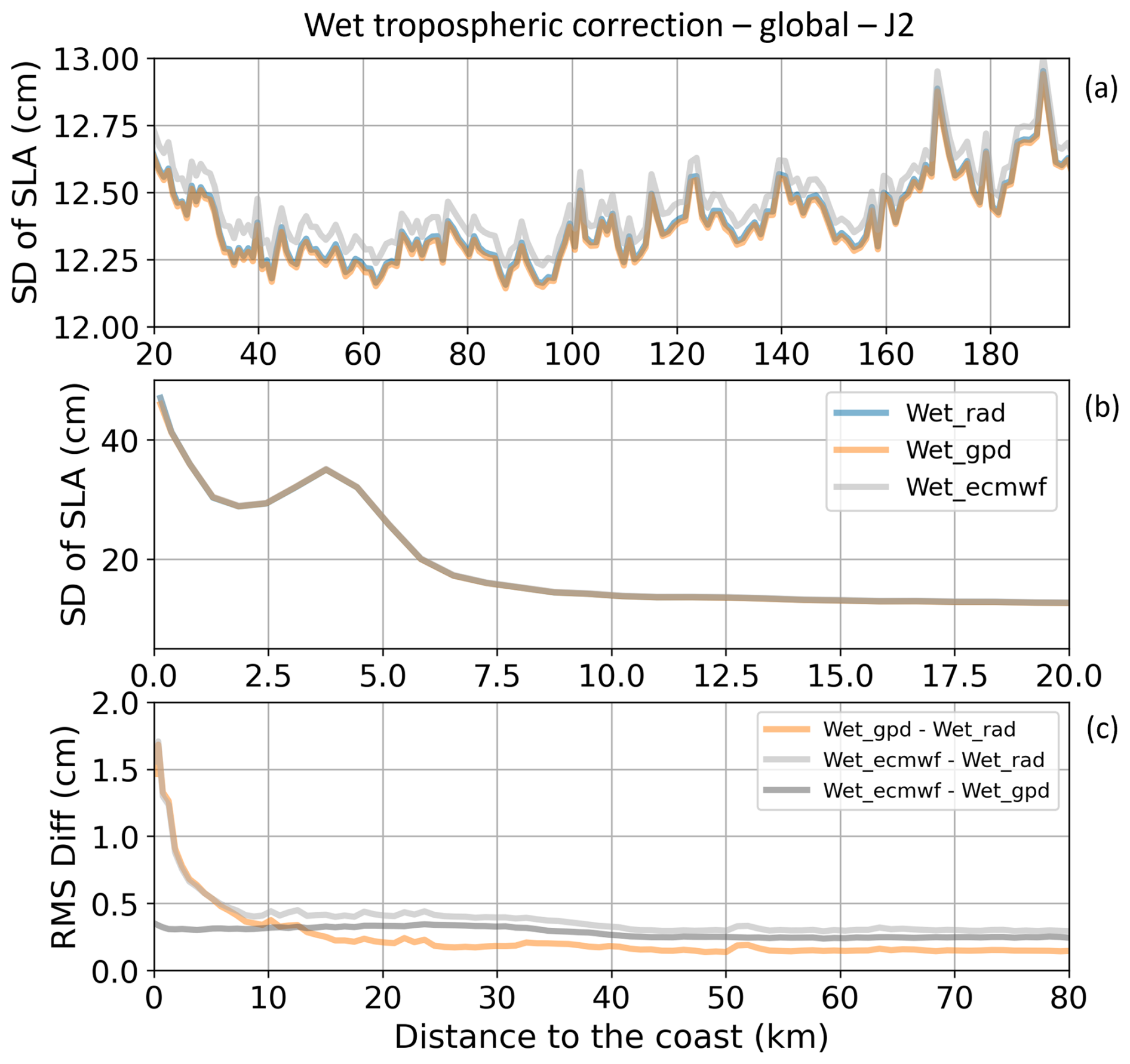
Figure 5 (a, b) Global mean of standard deviation values (in cm) of the SLA along all Jason-2 tracks for the period 27 September 2013 to 2 December 2016 when applying different WTC corrections. Results are represented as a function of the distance to the coast (in km) between 200 and 20 km (a) and between 20 and 0 km from the coast (b). (c) Global standard deviation of the differences in standard deviation values (in cm) of the SLA when applying different WTC corrections between 80 and 0 km from the coast.

As a conclusion of this section, Fig. 5 illustrates the progress that has been made in the WTC quality in nearshore regions. In 2011, Andersen and Scharroo (2011) reported a deterioration of half its quality at 30 km from the coast. Our results show that today, WTC uncertainties increase only 10 km from the coast (on average). Note however that this conclusion must be modulated by one consideration. The results associated with the radiometer solution might be different for altimetry missions which have not been reprocessed recently with the GDR product versions used here (see Table 1).

4.3 Ocean tide correction

Tides must be removed from altimetry measurements of sea level to avoid aliasing effects, as the satellite sampling period (9.9 d at best) does not allow us to resolve them. For this purpose, solutions from several global models can be used (a comprehensive summary can be found in Stammer et al., 2014, and in Zaron and Elipot, 2020, for more recent models). Global tidal models have largely evolved since the early days of altimetry, and today they all reproduce open-ocean tides with an accuracy of approximately 1–2 cm (Andersen and Scharroo, 2011). However, in shallow waters, they show larger differences (Ray et al., 2011) and may have errors larger than 10–20 cm (Ray, 2008) due to poorly resolved bathymetry and more complex tidal hydrodynamic features that are difficult to model. Different studies have shown that regional tidal models generally show better performances in coastal areas compared to global models (Cancet et al., 2018, 2022).

Here, in order to investigate this correction in coastal areas, we intercompare two global tidal models (EOT20 – Hart-Davis et al., 2021b; FES2014b – Lyard et al., 2021) and a CNES–NOVELTIS regional solution for the Mediterranean Sea, NEA and eastern Australia (Cancet et al., 2022). Because the resolution of the tidal model grid can have an impact on the tidal estimates in coastal regions, where the tidal spatial features are smaller, two versions of the global FES2014b model have been considered: interpolated (1) on a regular $\mathrm{1}/\mathrm{16}$° grid (i.e., about 7.5 km) as it is officially distributed and used in the operational altimetry products and (2) on the native unstructured grid, whose resolution is between ∼ 4 and ∼ 15 km in coastal regions. This part of the study has been restricted to the three regions where the regional solutions are available. Here we mainly present results for the NEA region, which is one of the coastal zones where the tides are the strongest and one of the most difficult to model in the world. Hence the results are more in contrast than for the two other regions. We only show results for Jason-2; all the results for the three regions and the two missions are available online (https://www.aviso.altimetry.fr/en/data/, last access: 8 November 2024).

Figure 6a and b show the SD of SLAs when applying each of the four tidal corrections in the NEA region. EOT20 is systematically about 0.5 to 2.5 cm above all the other solutions (the maximum of 2.5 cm is reached at 6–7 km from the coast, relative to the regional solution). In the open ocean, the difference between the three other solutions is below 0.5 cm, and this value increases towards the coast, reaching 1 cm at 3 km from the coast. The systematic difference between EOT20 and the other models may be at least partly due to its tidal spectrum which is smaller (17 tidal components available, 15 used for this study for reasons of incompatibility with the dynamic atmospheric correction; Hart-Davis et al., 2021a) than that of the FES2014b and regional models (all with 34 tidal components), thus removing less tidal signal from the altimetry SLA data. Indeed, the tidal components omitted in EOT20 are secondary, nonlinear elements that generally have larger amplitudes (at the millimeter or centimeter level) in shallow waters than in the deep waters of the open ocean (sub-millimeter).

The spread between the different SLA solutions obtained with these four tidal corrections is spatially variable, ranging between 1 and 2 cm up to 20 km from the coast (Fig. 6c). Below this distance the spread increases, with values reaching about 4 cm when considering only tidal solutions with the same spectrum and 5 cm when considering also the EOT20 model.

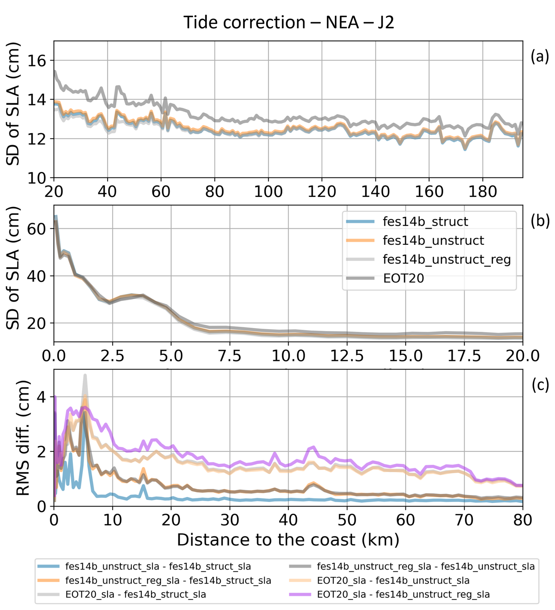
Figure 6 (a, b) Regional mean of standard deviation values (in cm) of the SLA along all Jason-2 tracks for the NEA region and for the period 27 September 2013 to 2 December 2016 when applying different ocean tide corrections. Results are represented as a function of the distance to the coast (in km) between 200 and 20 km (a) and between 20 and 0 km (b). (c) Regional standard deviation of the differences in standard deviation values (in cm) of the SLA in the NEA region when applying different tide corrections between 80 and 0 km from the coast.

Figure 7 represents the regional structure of the differences in the SD of SLAs corrected with the regional tidal solution and with the FES2014b global solution on the native unstructured grid (regional model minus global model). In reddish regions, FES2014b decreases the SD of SLAs more significantly; in blueish regions, it is the regional solution that reduces the SD of SLAs the most. The differences are on the order of a few millimeters in most parts of the NEA region, except in shallow areas where the tidal amplitudes are the largest (English Channel, Celtic Sea, southern part of the North Sea). In these regions, the differences provide negative values that vary significantly in space, from ∼ 1 cm to more than 3 cm.

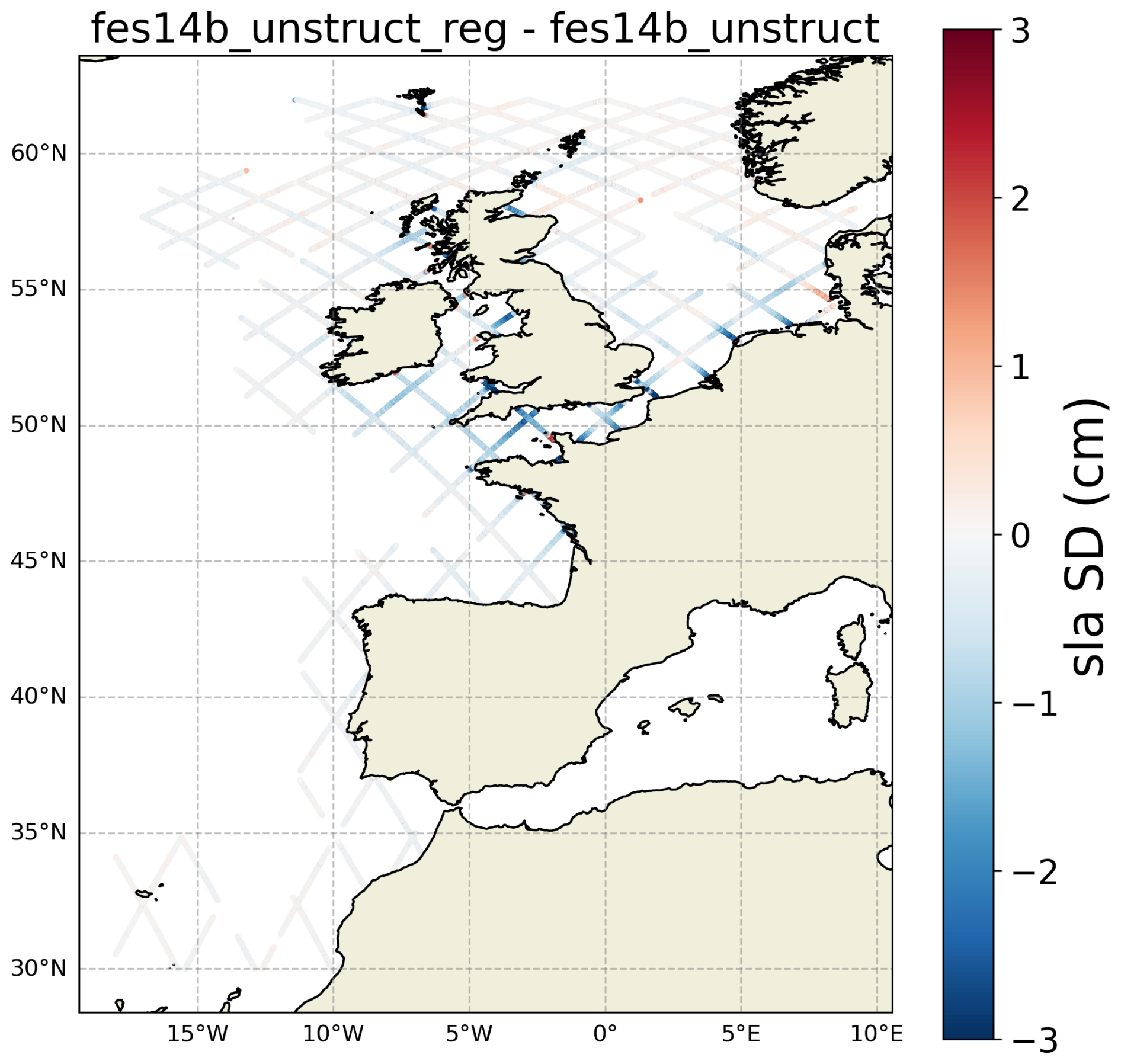
Figure 7 Regional map (NEA coastal area) of the differences in standard deviation values (in cm) of the SLA along all Jason-2 tracks for the period 27 September 2013 to 2 December 2016 when applying the CNES–NOVELTIS regional model compared to applying the FES2014b global tidal model on its native unstructured grid (regional model minus global model).

These results illustrate that although very significant progress has been made since studies such as Ray (2008), large uncertainties remain in ocean tidal corrections in coastal regions, linked to the model accuracy, but also for other reasons such as the tidal spectrum used. These uncertainties have complex spatial structures, associated with the tidal signal itself, which makes it meaningless to estimate them on a global scale. They are local in nature and can be a few millimeters in the Mediterranean Sea, a few centimeters in the Tasman Sea and on the northeastern Australian shelf (not shown), or even larger (English Channel).

To further quantify these geographical disparities, the four SLA solutions were compared with the equivalent series of sea level variations from tide gauges in the three study regions (see Sect. 2.3 and Fig. 2 for the details on the tide gauge selection). Here again, the comparison is made in terms of statistics: correlation and root mean square (rms) differences between the altimetry and in situ SLA observations (Fig. 8). The statistics are calculated for each 20 Hz altimetry point corresponding to the selection criteria specified in Sect. 2.3 and then averaged by tide gauge and by region. The results show that the choice of the tidal model in the SLA calculation has more impact in the NEA than in the two other regions. The Mediterranean Sea is a micro-tidal zone. However, concerning the Australia region, this result could be affected by the choice of tide gauge stations used for the analysis. Indeed, for our study we could select eight stations close to the Jason-2 and Jason-3 nominal ground tracks that happened to be located in regions with rather low tidal signatures. That may thus not be representative of other Jason-2 or Jason-3 ground tracks (or even other missions) that may sample the Australia region with larger tidal signals and larger uncertainties in the models.

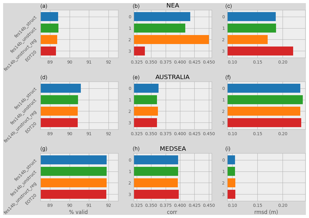
Figure 8 Regional averages of (a, d, g) the percentage of altimetry SLA data available in the time series for all the coastal zones selected, (b, e, h) correlation values, and (c, f, i) rms of the differences between the altimetry and in situ SLA observations.

4.4 Mean sea surface height

MSSH models correspond to the relative steady-state sea level and are obtained by time averaging and interpolating the instantaneous sea surface height data observed by the different altimeters over a finite period (Andersen and Knudsen, 2009). The precision and grid size of the existing MSSH solutions have been gradually improved and enhanced with the development of satellite altimetry. For wavelengths shorter than 250 km, their error is on the order of 1–2 cm² (Pujol et al., 2018), but it can become larger near the coasts where MSSH solutions suffer from the decrease in the quality and quantity of SLA data used to calculate them.

The investigation of the impact of coastal MSSH errors in the corresponding altimetry SLA data here involves comparing three models: CNES_CLS15 (Pujol et al., 2018), SIO (Sandwell et al., 2017) and CNES_CLS22 (Schaeffer et al., 2023). Figure 9a and b show the global average of the SD of SLAs as a function of the distance to the coast, applying each of the three MSSH solutions. The three plots are almost identical. Concerning the spread between the SLA solutions, it is below 0.5 cm in the open ocean (Fig. 9c). It starts to increase between 20 and 8 km from the coast, with values between 0.5 and 1 cm, and then rapidly amplifies in the last 8 km to the coast, with values reaching about 4 cm. It highlights that discrepancies between the MSSH solutions are concentrated in the coastal regions. We note that, close to the coast, the spread between the two CNES-CLS MSSH solutions is lower (2 cm) than the spread with the SIO MSSH model (4 cm).

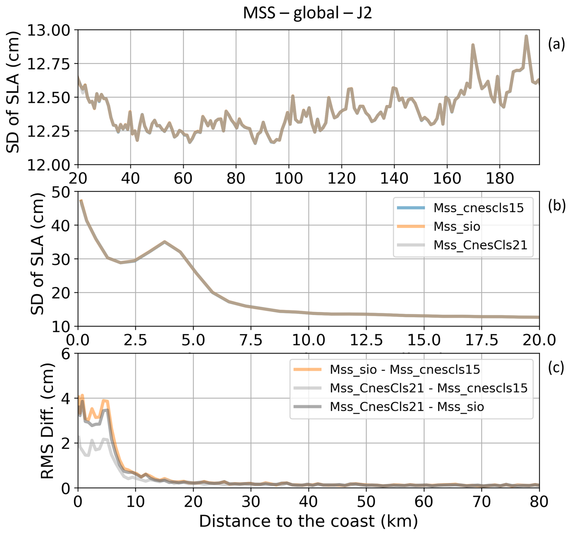
Figure 9 (a, b) Global mean of standard deviation values (in cm) of the SLA along all Jason-2 tracks for the period 27 September 2013 to 2 December 2016 when applying different MSSH solutions. Results are represented as a function of the distance to the coast (in km) between 200 and 20 km (a) and between 20 and 0 km from the coast (b). (c) Global standard deviation of the differences in standard deviation values (in cm) of the SLA when applying different MSSH solutions between 80 and 0 km from the coast.

4.5 Altimeter range and SSB

The accuracy of the altimeter range is directly related to the retracking method used. The latter consists of an analytical model fitted to the satellite waveform in order to derive geophysical information (the so-called retracking), including the range, the significant wave height and the wind speed. The SSB aims to correct the error in the satellite altimetry sea level measurements that is due to the presence of ocean waves at the ocean surface (Tran et al., 2021). Its estimation is based on empirical models (Gaspar et al., 2002) computed from the significant wave height and wind speed estimated during the retracking step. The altimeter range and the SSB used in the SLA calculation are then necessarily dependent since they are derived from the same analytical model. In the coastal zone, they are both impacted by the presence of more complex altimetry waveforms at about 10–15 km from the shore due to land contamination. This results in noisier fields at the output of the retracker (Andersen and Scharroo, 2011; Gommenginger et al., 2011). The SSB computation is also more complex in coastal areas because of the changing shape of the wave and wind fields (Dodet et al., 2019). In this section, these two SLA components (i.e., range and SSB) will first be analyzed together. We will then focus on the SSB alone for which several calculation methods exist for a given retracker.

The MLE4 2D retracking algorithm (Thibaut et al., 2010) is the standard method used for the operational processing of LRM altimetry waveforms over the ocean. However, when approaching the coast, as mentioned above, the presence of signals coming from land in the altimetry waveforms impacts the ability of MLE4 to retrieve accurate geophysical variables. Different algorithms have been developed during the past years to improve the SLA data retrieval in nearshore areas. This is the case of the ALES (Passaro et al., 2014) and Adaptive (Poisson et al., 2018) retracking algorithms. In this section, we will analyze the differences in SLA obtained when using the range and SSB derived from these three retrackers (MLE4, ALES and Adaptive) and the way they behave when approaching the coastline. Here we only show results for Jason-3 because, unfortunately, it turned out that a significant number of Jason-2 cycles were missing in the Adaptive dataset.

First, we compare the SLA estimates computed with the range–SSB couple associated with each of the retracking algorithms considered in the round-robin. For the MLE4 retracking, the SSB version considered here is the 2D dataset at 1 Hz (GDR standard) interpolated at 20 Hz. For the Adaptive and ALES retracking algorithms, the 2D SSB solution directly was computed at 20 Hz. For Jason-3, the global mean of the SD of SLAs is 14, 13.8 and 14.1 cm for MLE4, Adaptive and ALES, respectively (for more details and plots, see https://www.aviso.altimetry.fr/en/data/, last access: 8 November 2024). However, when we represent the SD of SLAs for the three retrackers as a function of the distance to the coast (Fig. 10a and b), we see that these average numbers can mask significant spatial differences, particularly in the last 10 km to the coast. Note that the statistics associated with MLE4 are not completely comparable to those of the other retracking algorithms below 10 km because the number of data available at the output of the MLE4 retracker drops by about 20%, whereas the number of data available at the output of ALES and Adaptive remains stable up to about ∼ 4–5 km from the coast (Fig. 10c).

Here again, the spread between the SLA solutions obtained with these three retracking algorithms (Fig. 10d) clearly increases when approaching the coast, reflecting an increase in the SLA uncertainty associated with uncertainties in range and SSB. The associated SD values of the differences are below 0.5 cm in the open ocean up to 60 km from the coast, then they range between 0.5 and 1.5 cm between 10 and 60 km, and they finally increase up to 4 cm in the last 10 km.

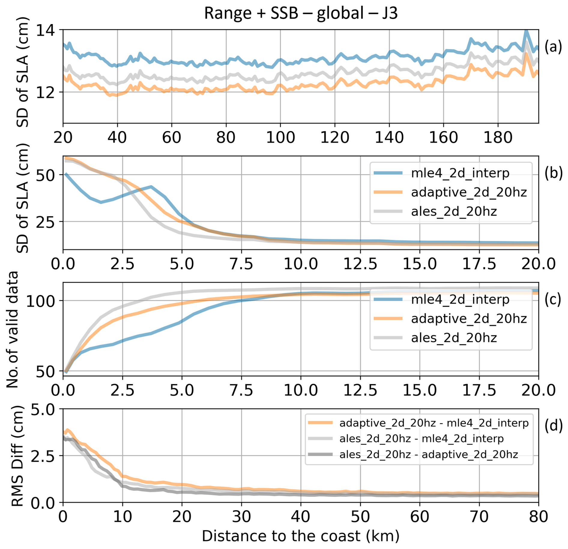
Figure 10 (a, b) Global mean of standard deviation values (in cm) of the SLA along all Jason-3 tracks for the period 17 February 2016 to 22 February 2019 when applying different retracking solutions for the range and the SSB corrections. Results are represented as a function of the distance to the coast (in km) between 200 and 20 km (a) and between 20 and 0 km from the coast (b). (c) Number of valid SLA data for each retracking algorithm between 20 and 0 km from the coast. (d) Global standard deviation of the differences in standard deviation values (in cm) of the SLA when applying different retracking solutions for the range and the SSB between 80 and 0 km from the coast.

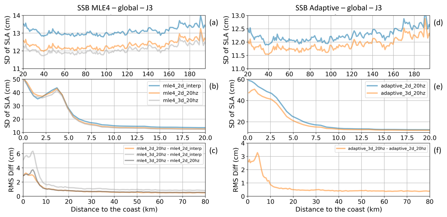
Figure 11 (a, b, d, e) Global mean of standard deviation values (in cm) of the SLA along all Jason-3 tracks for the period 17 February 2016 to 22 February 2019 when applying different solutions for the SSB corrections associated with the MLE4 (a, b) and Adaptive (d, e) retracking algorithms. Results are represented as a function of the distance to the coast (in km) between 200 and 20 km (a, d) and between 20 and 0 km from the coast (b, e). (c, f) Global standard deviation of the differences in standard deviation values (in cm) of the SLA when applying different SSB corrections associated with the MLE4 (c) and Adaptive (f) retracking algorithms between 80 and 0 km from the coast.

We now focus on the SSB correction. In the operational SLA processing, the reference correction is the MLE4 SSB calculated at 1 Hz and then interpolated at a higher rate (20 Hz). Passaro et al. (2018) showed that the computation of the SSB correction directly at 20 Hz improves the accuracy of the SLA estimate. Moreover, according to Tran et al. (2021), by using a 3D version of the SSB correction instead of the standard 2D version, we obtain an SLA variance reduction for the high-frequency signals. Here, we will intercompare the impact of 5 SSB solutions on the SLA computation as we approach the coast (Fig. 11). Three are associated with MLE4: the 2D version of the SSB computed at 1 Hz and interpolated at 20 Hz, the 2D version of the SSB directly computed at 20 Hz, and the 3D version of the SSB computed at 20 Hz (Fig. 11a, b, c). The two other solutions are associated with the Adaptive retracker: the 2D version of the SSB computed at 20 Hz and the 3D version of the SSB computed at 20 Hz (Fig. 11d, e, f). Note that we do not consider the ALES solution here as we want to focus on the impact of the SSB separately from that of the range. Hence we can only intercompare SSB solutions associated with a given retracker (only one ALES SSB solution available).

For the entire study area considered, for MLE4, the mean SD of the SLA obtained is 14 cm for the 2D SSB at 1 Hz, 13.2 cm for the 2D SSB at 20 Hz and 12.9 cm for the 3D SSB at 20 Hz (see https://www.aviso.altimetry.fr/en/data/products/, last access: 8 November 2024). For Adaptive, it reaches 13.8 and 12.8 cm for the 2D SSB at 20 Hz and 3D SSB at 20 Hz, respectively. These results show the strong impact of the SSB processing on the SLA estimates on a global scale and particularly the consequence of the interpolation from 1 to 20 Hz, as is commonly done when using the operational altimetry products, on the resulting SD values.

If we represent the SD of SLAs for the various SSB solutions as a function of the distance to the coast (Fig. 11a, b, d and e), we can see differences on the order of 1 cm between the solutions in the open ocean up to about 10 km from the coast. In the last 10 km, larger discrepancies are observed among the curves, showing different shapes from the values of SD of SLAs increase close to the coast.

The spread between the SLA solutions obtained with the various SSB corrections (Fig. 11c and f) provides an estimate of the uncertainties associated with the SSB, ranging from 1.8 to 6.2 cm in the last 10 km to the coast. This means that the available SSB solutions strongly disagree very close to the coast. However, the largest coastal discrepancies (more than 6 cm) are observed between the oldest (MLE4 SSB 2D 1 Hz interpolated at 20 Hz) and the newest (MLE4 SSB 3D directly computed at 20 Hz) approaches. When considering the 2D and 3D SSB solutions directly computed at 20 Hz, the maximum discrepancies are lower, on the order of 3.5 to 4 cm for both the MLE4 and Adaptive algorithms. The most recent approaches to calculating SSB thus appear to reduce the SLA uncertainty, and we can expect some further reductions in the future as works are still ongoing to improve this correction.

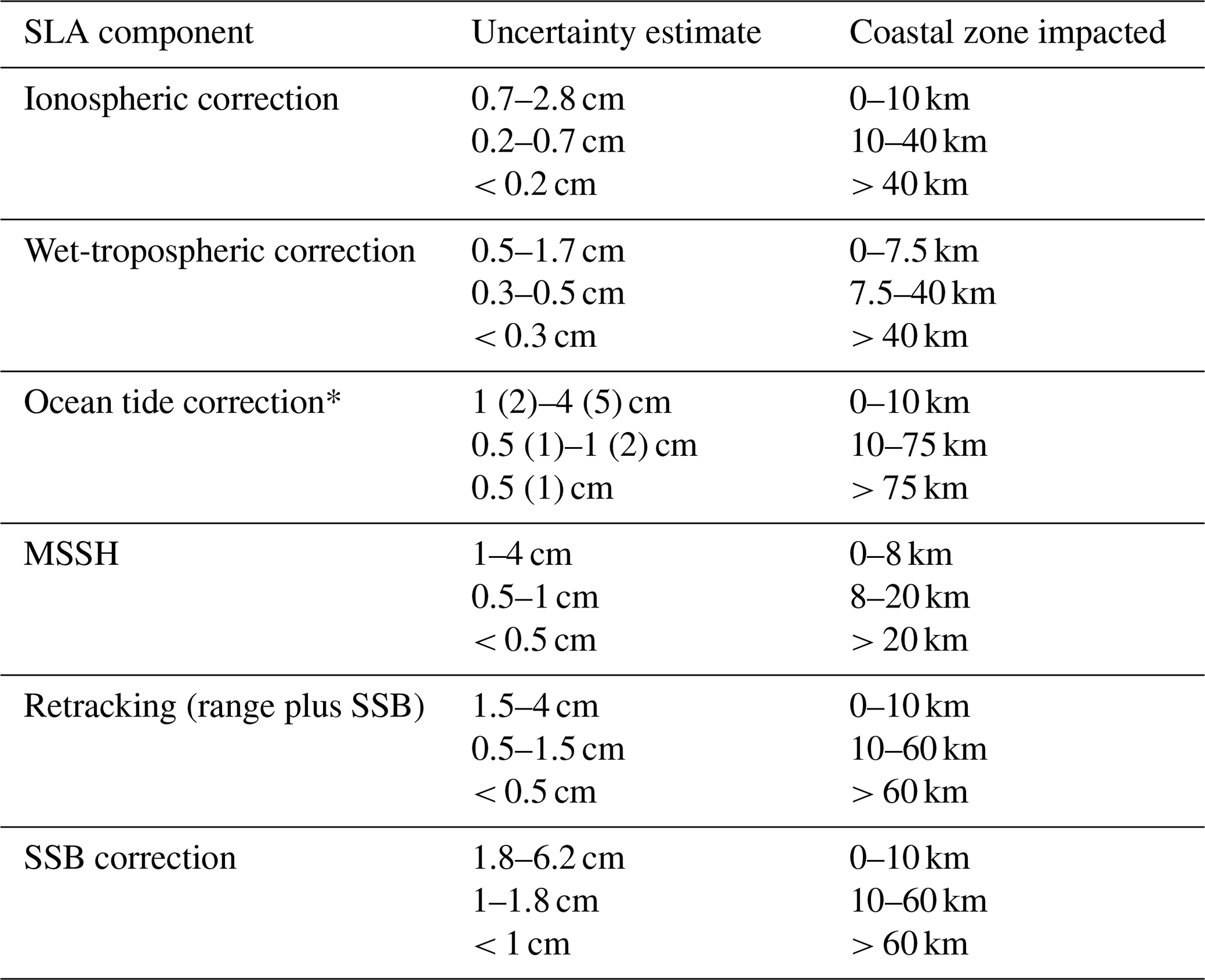
Table 2 SLA components included in the study (column 1), maximum spread of the differences in the SD (SLA) (uncertainty estimate) observed when we change the solution for this component (column 2) and oceanic region where these differences are observed (column 3). ^* For the ocean tide correction, the values in brackets correspond to uncertainty estimates considering the EOT20 model, while the other values correspond to the FES2014 and regional models only.

4.6 Synthesis of the results

We summarize in Table 2 the main results found in this study for the different SLA components. Beyond the near-coastal region, the biggest contributors to uncertainty in the LRM altimeter SLA are the SSB and the range, both associated with the retracker algorithms, generating an uncertainty of about 1 cm. Then comes the tidal correction with an associated uncertainty between 0.5 and 1 cm, depending on the tidal models that are considered (in particular, the extent of the tidal model spectra is a key player in the estimation of the associated uncertainties, as more tidal signal is removed from the altimeter SLA when using models with a richer spectrum). The MSSH also contributes on the order of 0.5 cm to the uncertainties in the estimated SLA in the open ocean. For the other components (ionospheric and wet-tropospheric corrections), the solutions tested generated difference envelopes of less than 0.3 cm.

For all components, the uncertainties in the estimated SLA start to slightly increase at some distance to the coast (75 km for the tides, 60 km for the range and SSB, 40 km for the ionospheric and wet-tropospheric corrections, 20 km for the MSSH), reaching between 0.5 cm (ionospheric correction) and about 2 cm (SSB, tides) at about 10 km from the coast. The largest uncertainties in the estimated SLA associated with these components are all observed in the last 7.5 to 10 km to the coast, where the spread between all the SLA estimates strongly increases, reaching several centimeters for all the components, from about 2 cm for the ionospheric correction to about 6 cm for the SSB.

In addition, these average uncertainty values mentioned in Table 2 hide significant spatial variations with levels that can be locally higher, for instance in areas of strong bathymetric gradient for the MSSH and of large tidal amplitudes or complex features for the tidal correction (Fig. 7). For the wet-tropospheric correction, this result is true provided that a recent version of the radiometric correction is used.

When we get very close to the coast, at around 10–15 km from land, the availability of the SLA components can play an important role in the statistics, with for instance some artificial drops in the SD of SLAs due to a lower amount of available data, as can be noticed for the altimeter range and SSB (Fig. 10b), with possible differences of several tens of centimeters that are beyond the amplitude of the oceanographic signals we want to observe. The choice of the retracker algorithm thus becomes really critical if we want to use altimeter data in the nearshore area.

It is also important to note that these uncertainty estimates are interlinked from one component to the other and are not independent from each other, as most of them are also based on satellite altimetry observations (e.g., SSB, MSSH, tidal models). The total uncertainty associated with all the components thus cannot be estimated as the direct sum of the uncertainty for each component.

Finally, this study does not aim to assess the accuracy of the SLA. It would only be possible by using co-located tide gauge observations as a reference. The results reflect the uncertainties in the estimated SLA related to errors in the processing and calculation algorithms. These uncertainties are quantified through the analysis of the SD of SLAs obtained using different approaches in the calculation. In altimetry, this is a classical diagnosis of the algorithm performance, considering that a solution performs well when it reduces the variability in the SLAs. As this study covers a wide range of algorithms, including the most recent and efficient algorithms available today to compute altimetry SLAs, it probably represents the best we can currently do in estimating altimeter uncertainties.

5 Conclusions

The contribution of satellite altimetry to scientific advances in the field of ocean dynamics is unique in the history of Earth observation from space (International Altimetry Team, 2021). It is now critical to improve and understand sea level observations from altimetry in coastal areas so that they can play a major role in coastal oceanography. This requires an understanding of the current sources of uncertainty in the data and then their reduction. In this study, we take advantage of the availability of several algorithms for most of the terms/corrections used in the calculation of the altimeter SLA to estimate the uncertainties associated when approaching the coast. We are focusing on LRM altimetry, which has the largest data history and the longest number of processing algorithms available. A round-robin exercise testing a total of 21 solutions for retracking radar altimeter data, correcting sea surface heights and finally deriving sea level variations has been performed. All solutions are evaluated through the same metrics, at both global and regional scales, and as a function of the distance to the coast. The results show that SLA uncertainties remain low and stable beyond 40–60 km from the coast, making them very reliable to use in this area. Within this distance, uncertainty values start to increase gradually. They can still be used with caution, especially if the ocean signal studied is larger than a few centimeters, up to 10 km from the coast. Then, they reach levels of magnitude above most ocean dynamic signals. In terms of origin, uncertainties in ocean tide models and in mean sea surface height models significantly contribute to the coastal SLA uncertainty budget in some regions. Concerning tidal models, despite major progress, the spatial resolution remains inadequate to take account of the dynamics of the most coastal tide (Hart-Davis et al., 2024). Concerning MSSH solutions, they are still poorly constrained near the coast due to the lack of SLA data to calculate them and their poorer quality (Pujol et al., 2018). The altimeter range and the SSB appear to be large contributors to SLA uncertainties in the open ocean, but within 10 km from the coastline, they become the limiting factor in the use of altimetry data. This is due to the complexity of radar echoes near the coast, which makes them much more difficult to model. If the result is that coastal users should give preference to altimetry datasets based on retrackers developed for coastal objectives, such as Adaptive and ALES, the remaining uncertainty levels underline the importance of further improvements in this domain.

Finally, it is important to keep in mind that the findings of this study are intrinsically related to the algorithms currently available to compute the altimeter SLA. They may significantly evolve in the future thanks to new methods and algorithms. We believe this work is important for better understanding and characterizing the current sources of errors and uncertainties in the altimetry measurements in coastal sea areas. This is the reason why the results obtained have already been transferred to the CNES operational computing center. In parallel, based on this study, we have started to work on the computation of sea level uncertainties that can be added to coastal altimetry products. This should greatly facilitate the use of these datasets by a wider scientific community. Note that even if this work was carried out with LRM altimetry data, part of the conclusions should also contribute to modern altimetry techniques such as SAR and SARIn, as all satellite altimetry missions share some common correction terms, such as tidal and MSSH models. Even with their increased observational capabilities, which are favorable for monitoring coastal zones, the way these new types of altimetry observations are processed and the methodologies used to calculate the various geophysical corrections remain critical steps to derive accurate and precise geophysical information.