An evaluation of the Arabian Sea Mini Warm Pool's advancement during its mature phase using a coupled atmosphere–ocean numerical model

A coupled atmosphere–ocean numerical model is used to examine the relative contributions of atmospheric and oceanic processes in developing the Arabian Sea Mini Warm Pool (MWP). The model simulations were performed for three independent years, 2013, 2016, and 2018, through April–June, and the results were compared against observations. The model-simulated sea surface temperature (SST) and sea surface salinity (SSS) bias were less than 1.75 °C and 1 psu, respectively; this bias was minimal in the MWP region. Moreover, the model simulated results effectively represented the presence of the MWP across the three different years. The mixed-layer heat budget analysis indicated that the net surface heat flux raised the mixed-layer temperature tendency of the MWP by a maximum of 0.1 °C d⁻¹ during its development phase. The vertical processes exerted a cooling impact on the temperature tendency throughout May and June with a maximum of −0.08 °C d⁻¹. Nonetheless, the decrease of net surface heat flux emerged as the dominant factor for the dissipation of the MWP. Further, four sensitivity numerical experiments were performed to investigate the comparative consequences of the ocean and atmosphere on the advancement of the MWP. The sensitivity experiments indicated that pre-April ocean conditions in years with a strong MWP resulted in a 136 % increase in MWP intensity in years when MWP SST was close to the climatology, which shows the primary role of oceanic preconditioning in determining MWP strength during strong-MWP years. Once the oceanic preconditions are met, the atmospheric conditions of weak-MWP years lead to an 82 % reduction in MWP intensity relative to normal years, highlighting the detrimental impact of atmospheric forcing under such circumstances. Atmospheric conditions, particularly wind, are critical in influencing the spatial evolution and dissipation of the MWP in the southeastern Arabian Sea (SEAS). A wind shadow zone, characterized by less production of turbulent kinetic energy that does not exist during weak-MWP years, facilitates the spatial expansion of the MWP in SEAS during moderate to strong-MWP years.

1 Introduction

The north Indian Ocean (NIO) associated ocean–atmosphere dynamics, including monsoons and cyclones, are well explored by researchers. One of the primary determinants in this interconnected process is the sea surface temperature (SST). During the pre-monsoon season, the southern region of the Arabian Sea experiences SST exceeding 28 °C, which is associated with the larger Indo-Pacific Warm Pool. However, the highest temperature is observed in the southeastern Arabian Sea (SEAS) from late April to May, before the onset of the Indian summer monsoon. These patches of warm water in the SEAS are often referred to as the Arabian Sea Mini Warm Pool (MWP) (Joseph, 1990; Rao and Sivakumar, 1999; Seetaramayya and Master, 1984; Shenoi et al., 1999). The MWP SST remains 0.5 to 1 °C higher than the surroundings during this time. Because the MWP SST stays at more than 30 °C, well above the minimal criteria for deep convection, it is thought to play a significant role in the Indian summer monsoon characteristics over Kerala (Deepa et al., 2007; Masson et al., 2005; Neema et al., 2012; Rao and Sivakumar, 1999).

Extensive studies have been conducted on the seasonal and interannual evolution of the MWP due to its noteworthy impact on regional climate dynamics (Akhil et al., 2023; Durand et al., 2004, 2007; Kurian and Vinayachandran, 2007; Mathew et al., 2018; Nyadjro et al., 2012; Rao and Sivakumar, 1999; Shenoi et al., 1999). According to Rao and Sivakumar (1999), the East India Coastal Current brings low-salinity water to the SEAS in winter, which causes strong stratification and leads to the formation of the MWP the following May. Shankar and Shetye (1997) explained the formation of the MWP in terms of the wave propagation phenomenon. The downwelling coastal Kelvin wave travels along India's east coast after the summer monsoon has passed, eventually reaching the SEAS in November–December. Later, it is deflected westward by the Rossby Wave, forming the “Laccadive High” (Bruce et al., 1994, 1998; Shankar and Shetye, 1997). The East India Coastal Current, triggered by the coastal Kelvin wave on India's east coast, brings low-salinity water to the SEAS and recirculates along the downwelling Laccadive High eddy in November and December. This low-salinity water leads to the formation of a barrier layer in the SEAS (Gopalakrishna et al., 2005; Hareesh Kumar et al., 2009; Masson et al., 2005; Murty et al., 2006; Shenoi et al., 1999). The barrier layer prevents the mixing of water above and below the thermocline (Lukas and Lindstrom, 1991) and traps the incoming shortwave radiation during the pre-monsoon season within the top few meters and thus increases the SST and leads to the MWP formation in next May (Hastenrath and Greischar, 1989). Masson et al. (2005) reported that the wintertime barrier layer intensifies the SST of the MWP by approximately 0.5 °C.

Hareesh Kumar et al. (2009) investigated the development of the MWP using the Princeton Ocean Model. They stated that salinity has a significant impact on the formation of the MWP. Using an ocean general circulation numerical model, Kurian and Vinayachandran (2007) discovered that the orographic influence of the Western Ghats acts as a wind barrier, increasing net surface heat flux and, hence, MWP intensity. According to Mathew et al. (2018), latent heat flux and incoming shortwave radiation, rather than wintertime freshening, influence the formation of the MWP. Recently, Akhil et al. (2023) found that subsurface dynamics during the preceding winter have very little influence on the development of the MWP.

Warm water can negatively affect the ocean ecosystem, particularly coral reefs (Abram et al., 2003; Doval and Hansell, 2000; Sarma, 2006). Given its proximity, any sudden increase in the intensity of the MWP could impact biological activity in the Laccadive High region. The MWP's impact also affects sound propagation dynamics (Hareesh Kumar et al., 2007). Despite the evident importance, the formation mechanism of the MWP remains a topic of ongoing scientific debate. The complex interplay of factors contributing to the genesis of the MWP, including winter salinity stratification and the presence of the Western Ghats, has been investigated in previous studies (Durand et al., 2004; Gopalakrishna et al., 2005; Hareesh Kumar et al., 2009; Kurian and Vinayachandran, 2007; Masson et al., 2005; Nyadjro et al., 2012). However, recent findings by Akhil et al. (2023) suggested that the influence of winter salinity stratification on the MWP genesis might be less significant than previously thought. Moreover, a limited number of studies have focused on the air–sea interaction during the mature phase of the MWP, highlighting the need for further research in this area. Hareesh Kumar et al. (2009) and Mathew et al. (2018) have explored these interactions, but comprehensive analyses remain sparse. Li et al. (2023) recently examined the Arabian Sea warm pool during its mature phase, emphasizing its seasonal and interannual variability using reanalysis datasets. While these studies contribute valuable insights, they primarily address variability over time rather than the specific processes driving the MWP's development and dissipation.

In this study, we examine the impact of the air–sea interaction on the progression of the Arabian Sea Mini Warm Pool using a coupled atmosphere–ocean numerical model. The coupled model employed in this study is calibrated for precise application on a seasonal timescale, which imposes limitations on the duration of simulations. Therefore, long-term simulations in each year are not feasible. Consequently, the present study focuses on configuring a regional coupled atmosphere–ocean numerical model to study the region-specific expansion and dissipation of the MWP. We also aim to elucidate the contribution of oceanic and atmospheric conditions to its growth over the years with distinct MWP intensity. The primary framework of the study is as follows: Sect. 2 provides an in-depth discussion of the data and methodology, including a detailed explanation of the coupled numerical model. Section 3 demonstrates the results along with the coupled model's ability to simulate temperature, salinity, and currents. Further, a few model sensitivity experiments have been incorporated to explore MWP characteristics and the influence of atmospheric and oceanic conditions across three different MWP events. Section 4 discusses the results and concludes the study with key findings.

2 Data and methodology

2.1 Data

We utilized the Advanced Very High Resolution Radiometer (AVHRR) SST dataset, which is a part of the NOAA Climate Data Record program product suite. This dataset combines in situ and satellite data from 1981 to the present using the optimal interpolation approach and is available at a daily timescale with a spatial resolution of 0.25° (Banzon et al., 2016). In this study, the coupled model's simulated SST is compared with the daily AVHRR SST data for the years 2013, 2016, and 2018. We used weekly sea surface salinity (SSS) data from the European Space Agency's Sea Surface Salinity Climate Change Initiative (CCI) to validate the model's simulated sea surface salinity (SSS). This global Level 4 dataset is derived from a multi-sensor combination (SMOS, Aquarius, and SMAP). It spans from 2010 to 2020, offering a horizontal resolution of 50 km and a weekly temporal frequency (Boutin et al., 2021). The model's ability to reproduce ocean surface currents is confirmed using OSCAR surface current data with a horizontal resolution of 0.33° and a temporal resolution of 5 d (Bonjean and Lagerloef, 2002). The numerical model-simulated vertical temperature and salinity are compared against AD10 buoy measurement data. AD10 is a moored buoy, and the National Institute of Ocean Technology (NIOT) is entrusted to deploy and collect the moored buoy data, later made available via the Indian National Centre for Ocean Information Services (INCOIS) data portal (https://incois.gov.in/portal/datainfo/mb.jsp, last access: 6 June 2024). The vertical resolution of the buoy data varies with depth.

2.2 Model details

The coupled atmosphere–ocean numerical model consists of the atmospheric model Advanced Research Weather Research and Forecasting (WRF–ARW) and the ocean model Regional Ocean Modeling System (ROMS). Both models are part of the Coupled Ocean–Atmosphere–Wave–Sediment Transport Modeling System (COAWST) (Warner et al., 2010). The model coupling toolkit (MCT) is used to couple the atmospheric model WRF-ARW and ocean model ROMS (Jacob et al., 2005). Previously, this coupled numerical model was used to study the air–sea interaction during tropical cyclones (Chakraborty et al., 2022; Prakash et al., 2018; Prakash and Pant, 2017, 2020; Zambon et al., 2014), coastal processes (Carniel et al., 2016; Olabarrieta et al., 2011, 2012; Ricchi et al., 2016), and monsoon deep depressions over the Bay of Bengal (Chakraborty et al., 2023).

The ROMS model is a free-surface, hydrostatic, three-dimensional primitive equation (i.e. Reynolds-averaged Navier–Stokes equation) ocean model widely used in estuarine, coastal, and basin-scale research. The primitive equations in the ROMS model are solved using boundary-fit orthogonal curvilinear coordinates on a staggered Arakawa C grid (Arakawa and Lamb, 1977). This model employs a terrain-following vertical sigma coordinate system (Haidvogel et al., 2000; Phillips, 1957; Song and Haidvogel, 1994) and incorporates a variety of advection techniques, such as second- and fourth-order center differences and third-order upstream biased method. Vertical mixing in ROMS is handled using either the local generic length scale closure technique (Umlauf and Burchard, 2003) or the nonlocal k-profile boundary layer formulation (Large et al., 1994). Horizontal mixing of momentum and tracers can occur at vertical levels or geopotential or isopycnal surfaces. Due to its very accurate and efficient physical and numerical algorithms, the ROMS model has been widely used to investigate the coastal, open-ocean, and biogeochemical processes (Nigam et al., 2018; Paul et al., 2023; Sandeep et al., 2018; Seelanki et al., 2021).

The WRF–ARW atmospheric model is a non-hydrostatic fully compressible model that predicts mesoscale processes using boundary layer physics schemes and various physical parameterizations (Skamarock and Klemp, 2008; Skamarock et al., 2008). On a horizontal Arakawa C grid and a vertical sigma-pressure coordinate, WRF–ARW estimates the wind momentum components, surface pressure, longwave and shortwave radiative fluxes, dew point, precipitation, surface sensible and latent heat fluxes, relative humidity, and air temperature. WRF is intended to serve and support atmospheric research and operational forecasting needs (Dai et al., 2013). Parameterization schemes are available in microphysics, cumulus parameterization, planetary boundary layer, surface layer, land surface, and longwave and shortwave radiations, with multiple options for each process. In the COAWST modeling system, the WRF code was modified to provide improved bottom roughness when computing bottom stress over the ocean (Warner et al., 2010). In addition to WRF and ROMS, the COAWST modeling framework also consists of wave and sediment transport models; however, these components are not used in this study.

2.3 Model configuration and experiment design

The atmospheric component of the coupled numerical model (i.e. WRF model) supports a variety of parameterization schemes. In our WRF configuration, we have incorporated the WRF Single-Moment 6-Class Scheme (Lim and Hong, 2010) as microphysics parameterization to represent grid-scale precipitation processes, the New Tiedtke scheme for cumulus parameterization that illustrates sub-grid-scale convection and cloud detrainment (Zhang and Wang, 2017), the Yonsei University Scheme (Hong et al., 2006) for planetary boundary layer physics, and the MM5 Similarity Scheme (Paulson, 1970). We have used the Unified Noah Land Surface Model (Tewari et al., 2004). At each time step, the atmospheric and land surface models calculate exchange coefficients and surface fluxes of the land or ocean layer and send them to the Yonsei University planetary boundary layer (Hong et al., 2006). The Dudhia shortwave scheme (Dudhia, 1989) is used for shortwave radiation parameterization, and the RRTM scheme (Mlawer et al., 1997) is used for longwave radiation parameterization. The WRF domain has an outer domain resolution of 60 km (18° S to 38° N and 25 to 95° E) and a nested domain with a 1:3 ratio (Fig. 1). It consists of 40 levels in the vertical direction. WRF is initialized with ERA5 data (Hersbach et al., 2020). The outer domain's lateral boundary condition is taken from ERA5 at 3 h intervals.

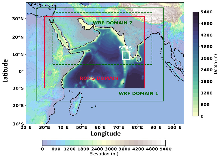
Figure 1 WRF and ROMS model domains. The WRF domain is the green box, while the red box shows the ROMS model domain. Two domains of WRF are shown in solid and dashed green lines. The white box is the southeastern Arabian Sea (core area of the MWP). Land elevation and ocean depth are shown in two different contours.

The ocean model ROMS employed in this study covers the Arabian Sea spanning 10° S–30° N and 30–85° E with a horizontal resolution of $\frac{\mathrm{1}}{\mathrm{6}}$. A terrain-following sigma coordinate system with 40 vertical levels was used, 20 of which are concentrated in the upper 200 m. The ETOPO2 with 2 arc min resolution data has been used to create the bathymetry data over the ROMS grid. The surface and bottom stretching parameters for sigma coordinates were set to θ_s=7 and θ_b=1.5, with a critical depth of 10 m. The initial conditions and lateral boundary forcings for ROMS were derived from SODAv3.4.2 (Carton et al., 2018) data, with a horizontal resolution of 0.5°×0.5° and a temporal availability of 5 d interval. Momentum and tracer particles were mixed horizontally along the geopotential surface. The nonlocal K-profile parameterization scheme (Large et al., 1994), which integrates the different unresolved processes associated with vertical mixing, was used to deal with vertical mixing. Horizontal and vertical advection of momentum were treated using third-order upstream and fourth-order centered advection schemes, respectively. The ROMS model employed 60 s baroclinic and 30 s barotropic time steps. Open boundary conditions for momentum and tracers on the southern and eastern boundaries used radiation schemes, allowing remote forcings from the Bay of Bengal and the southern Indian Ocean to influence the domain. Northern and western boundaries were closed in the ROMS model. Both models were initialized from April and simulated until June. A 1-month spin-up period was sufficient to establish the mixed-layer dynamics (the MWP extends till the mixed-layer depth; see Fig. S10).

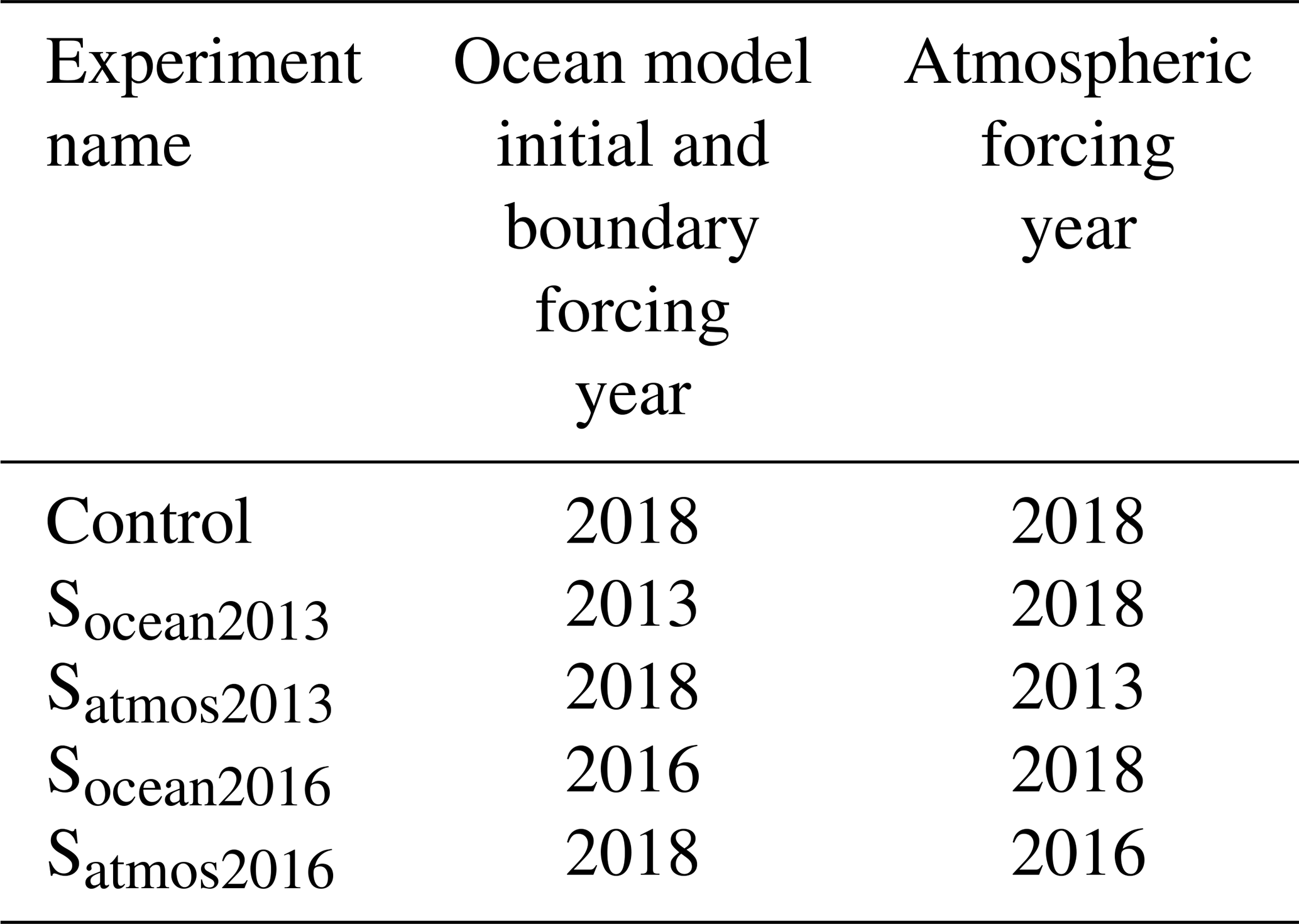
From the previous studies and our own experience (based on our several background experiments), we have observed that the coupled atmosphere–ocean numerical model (part of the COAWST model) would be more accurate if the simulation was up to the seasonal scale. Therefore, to assess the MWP using this coupled model, we ran the model for about 80 d for three independent years (2013, 2016, and 2018) which had distinct MWP characteristics (based on the interannual variation of the MWP area; see Fig. S1 in the Supplement). At every 15 min, the WRF and ROMS models interchange variables. While SST is the sole variable that is transferred from ROMS to WRF, other parameters, including 2 m air temperature, mean sea level pressure, 10 m u and v wind velocity, longwave and shortwave radiation, rainfall, and relative humidity, are exchanged between WRF and ROMS (readers are referred to Warner et al., 2010, for more details regarding the coupled model). Each run is initialized separately on 1 April and run to 20 June each year, and the output is saved at a daily frequency. The first month of each simulation was used for spin-up and is not included in the analysis (except for the mixed-layer heat budget analysis; Fig. 11). We named this set of runs the control experiment (CNTRL), where we used the SODA and ERA5 data for actual oceanic and atmospheric conditions. Later, to investigate the factors contributing to the evolution of the MWP, we designed and performed four idealized numerical experiments using the coupled atmosphere–ocean model with a one-way coupling mode. We modified the oceanic and atmospheric conditions in these experiments as detailed in Table 1. In 2018, the MWP area was closer to climatology (Fig. S1). Hence, this year is used as the base year, and in all four sensitivity experiments, the forcings of the two other years are fed into the 2018 control run.

Table 1 List of model sensitivity experiments.

2.4 Mixed-layer heat budget

The mixed-layer heat budget provides a detailed analysis of factors that can contribute to the change in the mixed-layer temperature and is calculated using the formula outlined in Akhil et al. (2023), Foltz and McPhaden (2009), Girishkumar et al. (2017), Nyadjro et al. (2012), Prakash and Pant (2017), Stevenson and Niiler (1983), and Vialard et al. (2008), and it is given as follows:

$$\begin{array}{}\text{(1)}& \begin{array}{rl}{\displaystyle \frac{\partial T}{\partial t}}=& {\displaystyle \frac{Q_{\mathrm{net}}}{\mathit{\rho }{C}_{p}h}}-\left(u{\displaystyle \frac{\partial T}{\partial x}}+v{\displaystyle \frac{\partial T}{\partial y}}\right)+H\left[W_{-h}+{\displaystyle \frac{\partial h}{\partial t}}\right]\\ & \left[{\displaystyle \frac{T_h-T}{h}}\right]+\mathrm{residuals}.\end{array}\end{array}$$

Different terms in the above equation's right-hand side (RHS) contribute to temperature tendency differently; the first term on the RHS is the contribution from net surface heat flux, the second is from horizontal advection, and the third is from vertical process and entrainment. T is the average temperature of the mixed layer, t is the time (in days), and h is the mixed-layer depth (MLD). Meridional and zonal velocities at MLD are given by u and v. Q_net is the net surface heat flux. Here, we have not considered the penetrative shortwave radiation below the MLD. H is the Heaviside step function and is expressed as H=0 if $\left[W_{-h}+\frac{\partial h}{\partial t}\right]<\mathrm{0}$ or H=1 if $\left[W_{-h}+\frac{\partial h}{\partial t}\right]>\mathrm{1}$. W_−h is the vertical velocity. T_h is the temperature just below (5 m) the depth of the MLD. The residual term represents contributions from other processes, such as diffusion. The units of all the terms here are in °C d⁻¹. In this study, the depth at which the subsurface temperature decreases by 1 °C as compared to the surface is used as the isothermal-layer depth (ILD) (Kara et al., 2000; Shee et al., 2019; Sprintall and Tomczak, 1992). The MLD is calculated following Shee et al. (2019) as follows:

$${\mathit{\sigma }}_{t(z=h)}={\mathit{\sigma }}_{t(z=\mathrm{0})}+\mathrm{\Delta }T{\displaystyle \frac{\mathrm{d}{\mathit{\sigma }}_t}{\mathrm{d}T}},$$

where ΔT is the 1 °C temperature criteria for ILD and $\frac{\mathrm{d}{\mathit{\sigma }}_t}{\mathrm{d}T}$ is the coefficient of thermal expansion.

2.5 The production of turbulent kinetic energy (P_TKE)

The production of turbulent kinetic energy (P_TKE) is used to understand the convective mixing caused by the relative contributions of wind stress (wind-forced momentum flux), freshwater flux (E−P) (haline buoyancy flux), and net surface heat flux (thermal buoyancy flux) (Shankar et al., 2016). P_TKE is calculated using the expression given in Han et al. (2001) and Rao et al. (2002) and expressed as follows:

$$\begin{array}{ll}{\displaystyle }{P}_{\mathrm{TKE}}=& {\displaystyle }\mathit{\rho }{u}_{*}^{\mathrm{3}}+\left[-{\displaystyle \frac{\mathit{\alpha }\mathrm{0.5}gk\mathrm{ML}D{Q}_{\mathrm{net}}}{C_p}}+\mathrm{0.5}\mathit{\rho }gk\mathrm{ML}D\mathit{\beta }\right.\\ {\displaystyle }& {\displaystyle }\left.(E-P)S_{\mathrm{0}}\right],\end{array}$$

where $u_{*}=\sqrt{\frac{\mathit{\tau }}{\mathit{\rho }}}$ is the frictional velocity, τ is the wind stress, ρ is the density of the seawater (1026 kg m⁻³), k=0.42 is the von Kármán constant, and g is the acceleration due to gravity. E is the evaporation rate, and P is the precipitation. S₀ is the salinity of the ML. Q_net is the net surface heat flux. The thermal expansion coefficient (α) and haline contraction coefficient (β) are taken to be $\mathit{\alpha }=-\mathrm{0.00025}$ K⁻¹ and β=0.00785 psu⁻¹, respectively, following studies by Shankar et al. (2016) and He et al. (2020). C_p (=4187 J kg⁻¹) is the ocean's specific heat capacity. The first term on the right-hand side of the above equation represents P_TKE due to wind stirring. The first term in the bracket is the P_TKE due to thermal buoyancy representing the effect of net surface heat flux, and the second term is P_TKE due to the haline buoyancy, which indicates the impact of freshwater change. The wind-stirring term, by definition, cannot be negative. A positive thermal buoyancy flux implies that heat is lost from the ocean, which causes MLD to deepen. On the other hand, the positive haline buoyancy flux causes more evaporation, which leads to an increase in MLD due to increased salinity (He et al., 2020; Shankar et al., 2016; Shee et al., 2019).

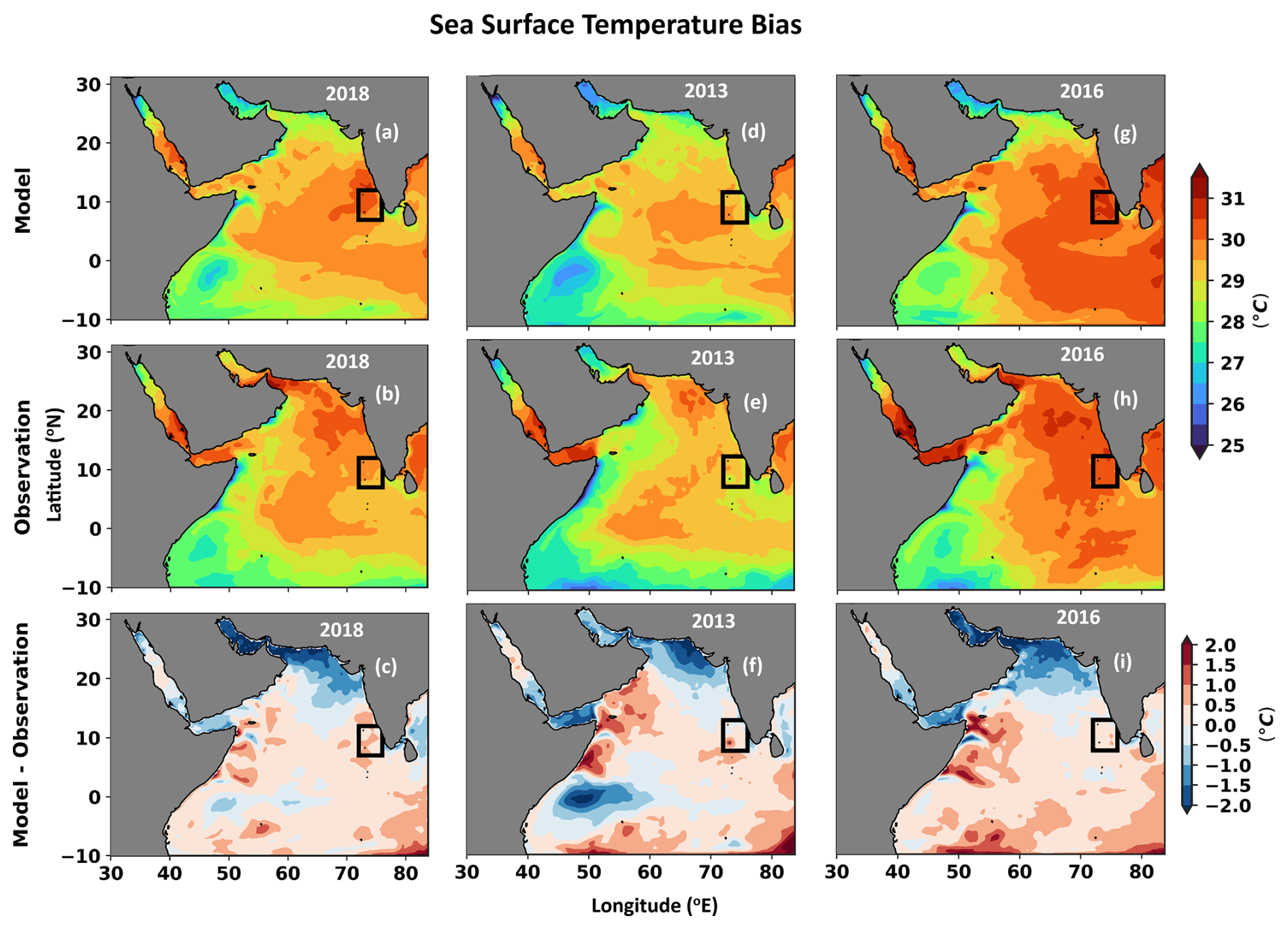
Figure 2 Comparison of model-simulated sea surface temperature (SST) and NOAA-AVHRR surface temperature. Panels (a), (d), and (g) depict model-simulated SST for the years 2018, 2013, and 2016, respectively. Panels (b), (e), and (h) display NOAA-AVHRR SST for the corresponding years. Panels (c), (f), and (i) illustrate the SST difference between model output and observation. The black box delineates the domain of interest, i.e. the MWP core region. The mean results and bias are shown for each of the three years, averaged from 1 May to 20 June.

3 Results

3.1 Model validation

Figures 2–4 compare the coupled model's simulated SST, SSS, and current to observation data in 2018, 2013, and 2016. The mean results and bias are then shown for each of the three years from 1 May to 20 June. The simulated SST effectively captured the cold SST along the Somali coast across all the examined years, firmly aligning with AVHRR SST data (Fig. 2). The SST bias remained within 1.5–2 °C in all three experiments except in the northern Arabian Sea and along the Somali coast. In the north Arabian Sea, a cold SST bias and a warm SST bias near the Somali coast of more than 1 °C are observed. In the tropical western Indian Ocean, a cold SST bias was also witnessed in 2013. Despite this, the SST bias remained consistent across the study period, with a minimal bias in the SEAS region (black box in Fig. 2). The model-simulated surface salinity revealed a pronounced high-salinity tongue in the northern Arabian Sea, a feature similarly observed in the ESA salinity data (Fig. 3). The coupled model effectively reproduced the low-salinity water in the SEAS, with the salinity bias being primarily within 0.5 psu across the entire domain, except for a few isolated areas reaching 1 psu. The Indian Ocean is well known for its seasonally reversing monsoon current. The West India Coastal Current (WICC) transports high-salinity water from the northern to the southern Arabian Sea in May and June and is the primary driver of inter-basin mass transport (Schott et al., 2009; Schott and McCreary, 2001; Shankar et al., 2002). The model-simulated surface currents accurately captured the WICC between May and June for all three years (Fig. 4). Furthermore, the representation of the summer monsoon current in the simulation was commendable (not shown here).

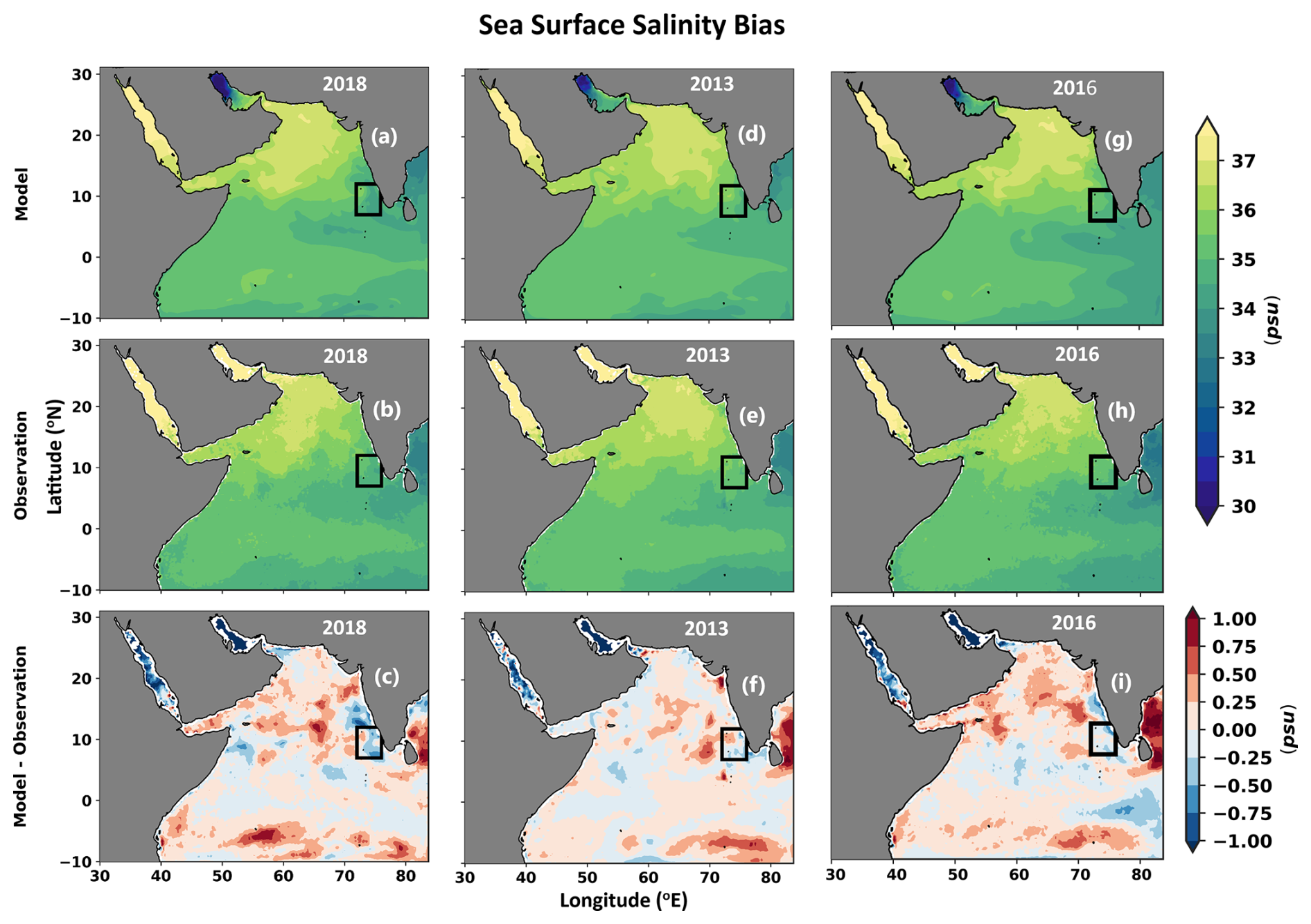
Figure 3 Comparison of model-simulated sea surface salinity (SSS) and ESA-observed SSS. Panels (a), (d) and (g) depict model-simulated SSS for the years 2018, 2013, and 2016, respectively. Panels (b), (e), and (h) display observed SSS for the corresponding years. Panels (c), (f), and (i) illustrate the SSS difference between the model output and observation. The black box delineates the domain of interest, i.e. the MWP core region. The mean results and bias are shown for each of the three years, averaged from 1 May to 20 June.

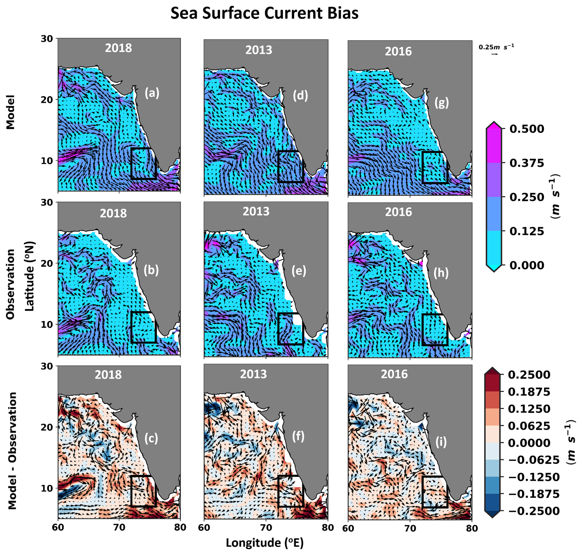
Figure 4 Comparisons of model simulated currents against OSCAR surface current. The first column from the left (a–c) is for 2018, the second is for 2013 (d–f), and the last is for 2016 (g–i). As the MWP forms near the western coast of India, the current patterns are shown in the adjacent region and not the whole model domain. Panels (c), (f), and (i) illustrate the difference between the resultant current and the direction between model output and observation. The black box delineates the domain of interest, i.e. the MWP core region. The mean results and bias are shown for each of the three years, averaged from 1 May to 20 June.

The coupled model's temperature and salinity profiles were confirmed against buoy measurements at the AD10 location (10.25° N, 72.25° E) (Fig. S2). We utilized the model's nearest point to the AD10 location to serve this purpose. Before validation, the model-simulated data are interpolated to the vertical resolution of the AD10 buoy data. The AD10 buoy data were available at an hourly timescale from 2012 to 2020 and at a 3 h frequency in 2021. Except for 2016, the AD10 temperature contains data gaps (Figs. S3–S5). In 2018, the model temperature had a cold bias below 50 m depth at the buoy location. In 2013 and 2016, the model's simulated temperature had a positive bias of less than 1 °C within the top 50 m. Although the vertical temperature is consistent with the AD10 buoy data, the model-simulated salinity data indicated more discrepancies in 2018. Aside from that, the model's represented salinity stayed within 1 psu bias in 2013 and 2016, with only a few areas exceeding this limit in 2013. The MWP does not extend beyond the mixed-layer depth (Akhil et al., 2023, and Fig. S10), and our model-estimated temperature and salinity remain in excellent accord within this depth. To further examine the vertical temperature performance of the model, we conducted a detailed temporal correlation analysis of the simulated temperatures for three distinct control experiments corresponding to the years 2018, 2013, and 2016. This analysis is performed against observational data obtained from the AD10 buoy location, with calculations made at various depths, specifically at 1, 5, 10, 15, 20, 30, 50, and 100 m. The results of this statistical assessment are graphically represented in a Taylor diagram (Fig. 5). The points at 50 m depth are out of the range of axes for 2013. Across all three control experiments, the standard deviation of the simulated temperature values generally ranged between 0.3 and 1.5, with a few exceptions at certain depths. Additionally, the correlation coefficient between the model simulations and the buoy observations varied from 0.5 to 0.98, indicating a moderate to strong agreement depending on the depth considered.

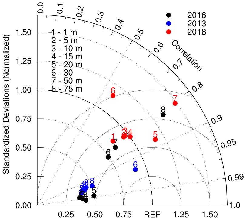
Figure 5 Taylor diagram showing the temporal correlation and standard deviations of the model-simulated temperature profile from the three years of model experiments with respect to measurements at the buoy AD10.

3.2 Ocean surface characteristics during various phases of the Arabian Sea Mini Warm Pool

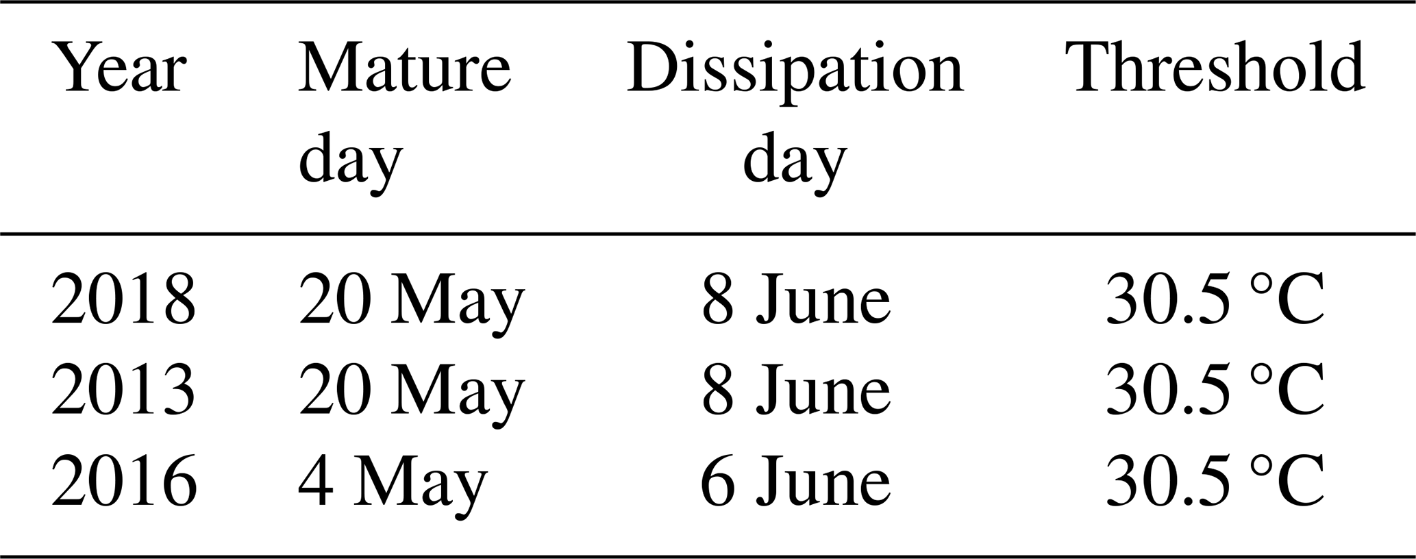
Figure 6 shows the model-simulated SST, wind stress, and salinity during the mature and dissipation days of the MWP. The mature day of the MWP is characterized by the day when SST within the MWP core (shown by the white box in Fig. 1) reaches its highest magnitude in May (Table 2). The dissipation day is determined when the MWP SST equates that of the surrounding water following its mature phase. In addition, the days from the mature to the dissipation day are termed the dissipation phase. Previous studies (Li et al., 2023; Rao and Sivakumar, 1999; etc.) have used 30 °C to identify the MWP. A consistent bias of 0.5 °C is noticed in SEAS; hence, our study used a threshold of 30.5 °C to detect the MWP. In 2018, the SST within the MWP core reached above 31 °C on 20 May, after which it gradually decreased (Fig. 6a–c). During the mature day in 2018, wind stress over the SEAS was low compared to its surroundings, but wind speed increased considerably afterward. Subsequently, the MWP SST matched the temperature of the surrounding sea by 8 June. Despite the absence of the MWP in 2013, the same MWP mature and dissipation day as in 2018 was used for demonstrative purposes (as shown in Fig. 6d–f). In 2016, the MWP matured on 4 May with a larger spatial area than the previous two years (Fig. 6g–i). During the mature day, the wind stress was minimal in the southern Arabian Sea (Fig. 6g). Once the wind stress escalated, the MWP entirely dissipated by 6 June 2016 (Fig. 6h and i).

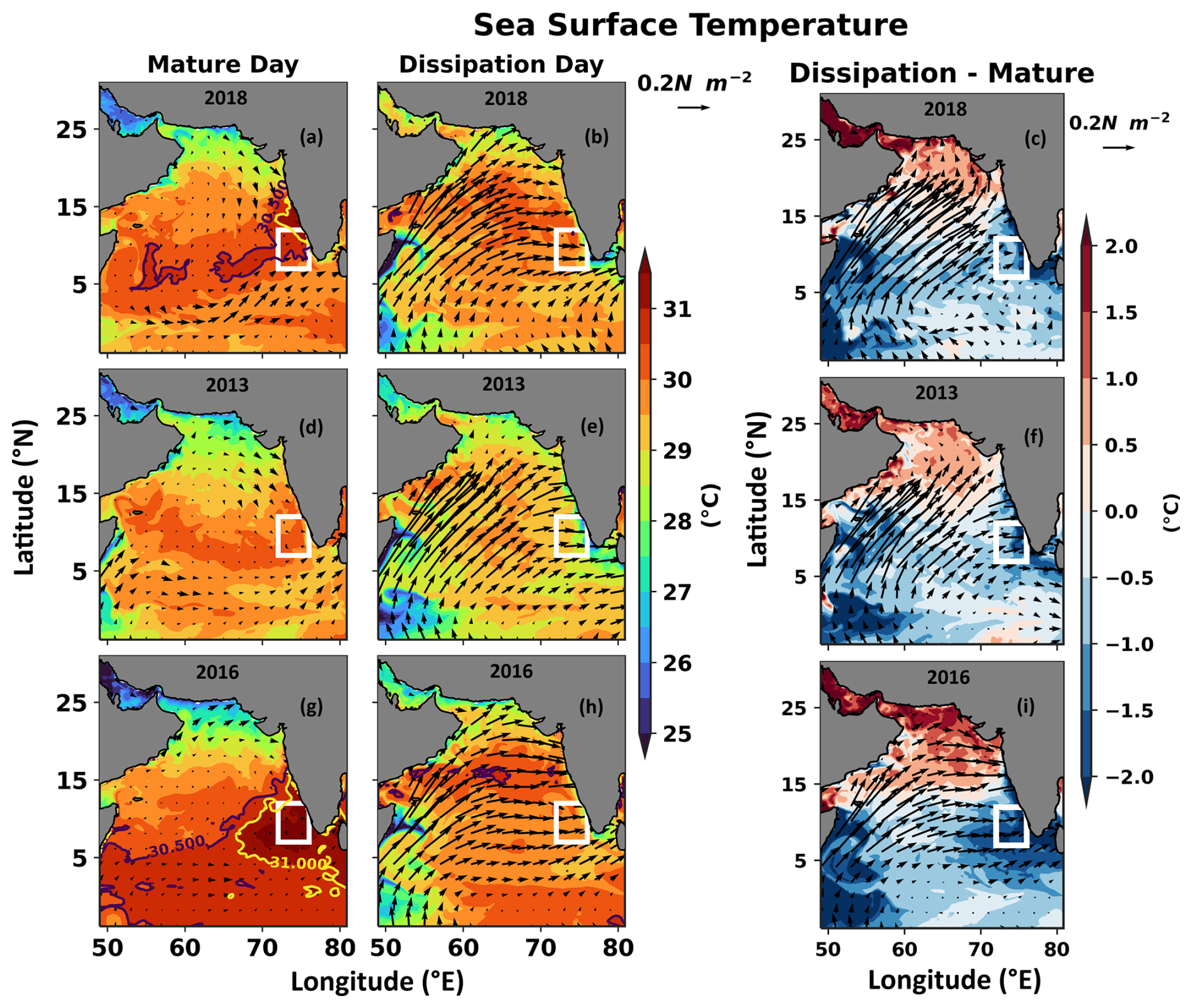
Figure 6 Comparison of SST overlaid by wind stress on mature and dissipation days (see Table 2 for details) in 2018 (a–c) (MWP strength close to climatology), 2013 (d–f) (MWP was absent), and 2016 (g–i) (MWP was intense). (c), (f), and (i) show the distinction between dissipation and mature days. The MWP's mature days are 20 May 2018, 20 May 2013, and 4 May 2016. The MWP's dissipation days are 8 June 2018, 8 June 2013, and 6 June 2016. The black and yellow contours represent 30.5 and 31 °C, respectively. The white box is the core MWP region.

Table 2 Details of mature and dissipation days in each year with the threshold used to identify the MWP.

Salinity in the vicinity of the MWP was lower during its mature day (<34 psu except in 2013) but increased during its dissipation day (>35.2 psu) (Fig. 7a–i). In the MWP core region, salinity was notably lower in 2018 compared to the other two years (Fig. 7a). In 2016, while the MWP was in its mature stage, low-salinity water (less than 34 psu) was detected south of SEAS, slightly outside the core MWP area (Fig. 7g). The salinity was higher in the SEAS during the mature day in 2013 as compared to 2016 and 2018.

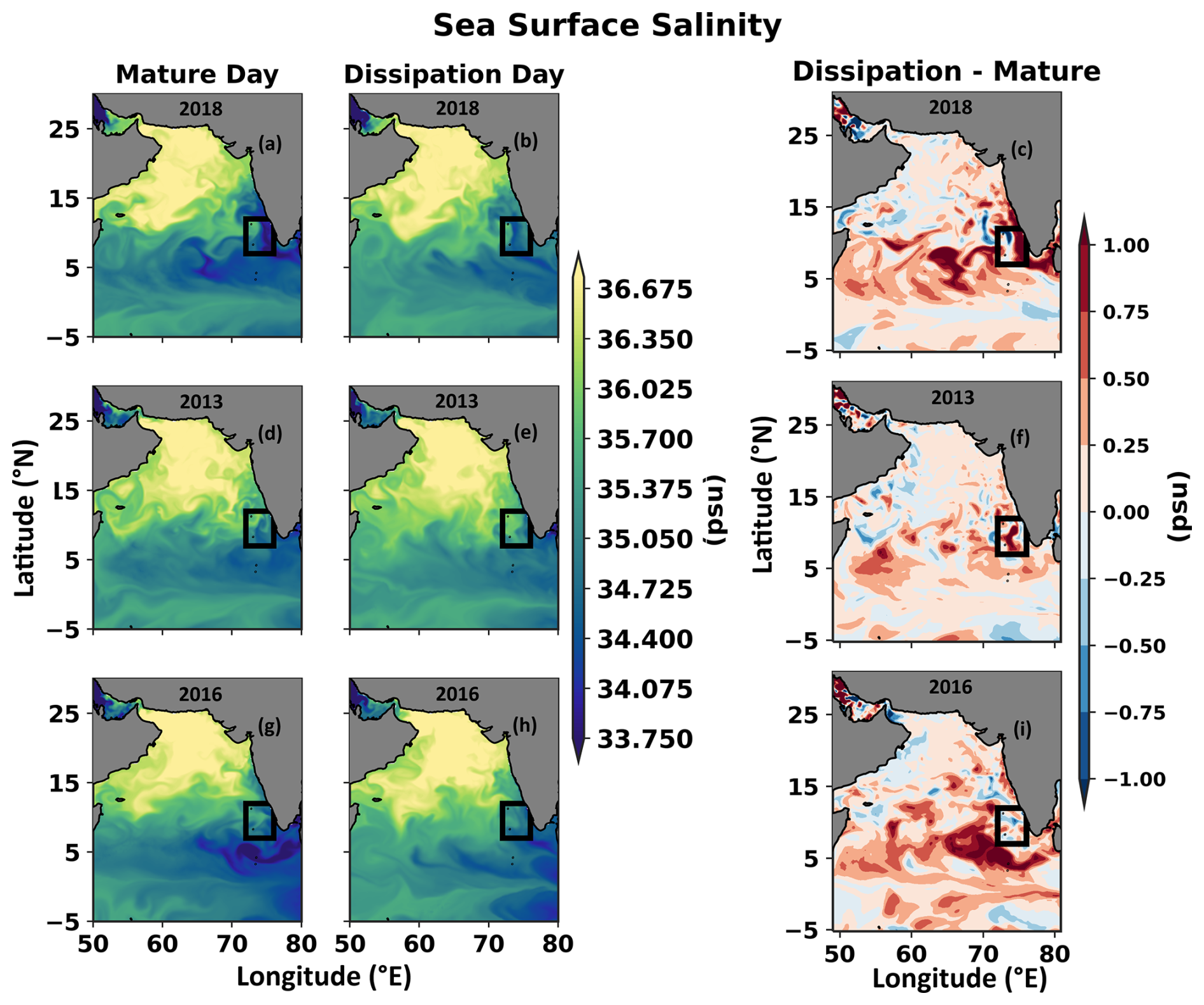
Figure 7 Comparison of sea surface salinity on mature and dissipation days (see Table 2 for details) in 2018 (a–c) (MWP strength close to climatology), 2013 (d–f) (MWP was absent), and 2016 (g–i) (MWP was intense). (c), (f), and (i) show the distinction between dissipation and mature day. The MWP's mature days are 20 May 2018, 20 May 2013, and 4 May 2016. The MWP's dissipation days are 8 June 2018, 8 June 2013, and 6 June 2016. The black box is the core MWP region.

On the mature day of the MWP, there was a positive net surface heat flux across the Arabian Sea except for its southern flank (Fig. 8a, d, and g). However, as wind stress intensified during the dissipation phase, the net surface heat flux in the Arabian Sea transitioned to negative values in all the years (Fig. 8c, f, and i). Subsequently, four elements of the net surface heat flux are examined to understand its impact on the regional growth of the MWP in SEAS (Figs. S6–S9). The shortwave radiation flux was positive and contributed majorly to the net surface heat flux. Because of the clear sky, the shortwave radiation was higher in April–May (Li et al., 2023). However, once the southwesterly wind strengthened, the subsequent cloudiness blocked the incoming shortwave radiation flux. Consequently, the shortwave radiation flux in the SEAS reduced on dissipation day (Fig. S6c, f, and i). The exchange of energy between the atmosphere and ocean is facilitated by turbulent processes, such as sensible and latent heat flux (Large and Pond, 1981). As the wind speed increased, the loss of the latent heat flux increased from the mature to the dissipation day in all the years (Fig. S8c, f, and i).

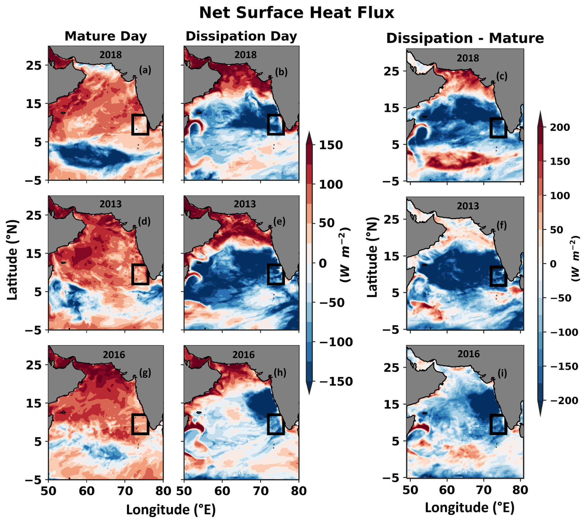
Figure 8 Same as Fig. 7 but for net surface heat flux.

3.3 Causative factors

3.3.1 The role of the atmosphere and ocean in the formation of the MWP

This section examines the relative contributions of the ocean and atmosphere to the development of the MWP through four sensitivity experiments (see Table 1 for details). In the S_ocean2013 and S_ocean2016 experiments, the ocean initial and boundary conditions from 2013 and 2016 replace those in the 2018 control experiment, respectively. The MWP remains very strong (weak) in the S_ocean2016 (S_ocean2013) experiment and reaches its maximum extent on 20 May (Fig. 9a and b are compared with Fig. 9c). An intense MWP was developed in the 2016 control experiment, and a similar MWP is also seen in S_ocean2016. The initial mean pre-April ocean temperature in SEAS (initial condition temperature is averaged within the white box in Figs. 9 and 10 and to the MLD) was 0.35 °C higher in 2016 (0.15 °C lower in 2013) compared to 2018. Following the initial conditions, the MWP core temperature within the MLD was 0.6 °C higher in S_ocean2016 (0.3 °C lower in S_ocean2013) compared to the 2018 control simulation during the mature day (Fig. S10d and e are compared with Fig. S10a). These results indicate that the pre-April ocean conditions strongly influence the intensity of the MWP.

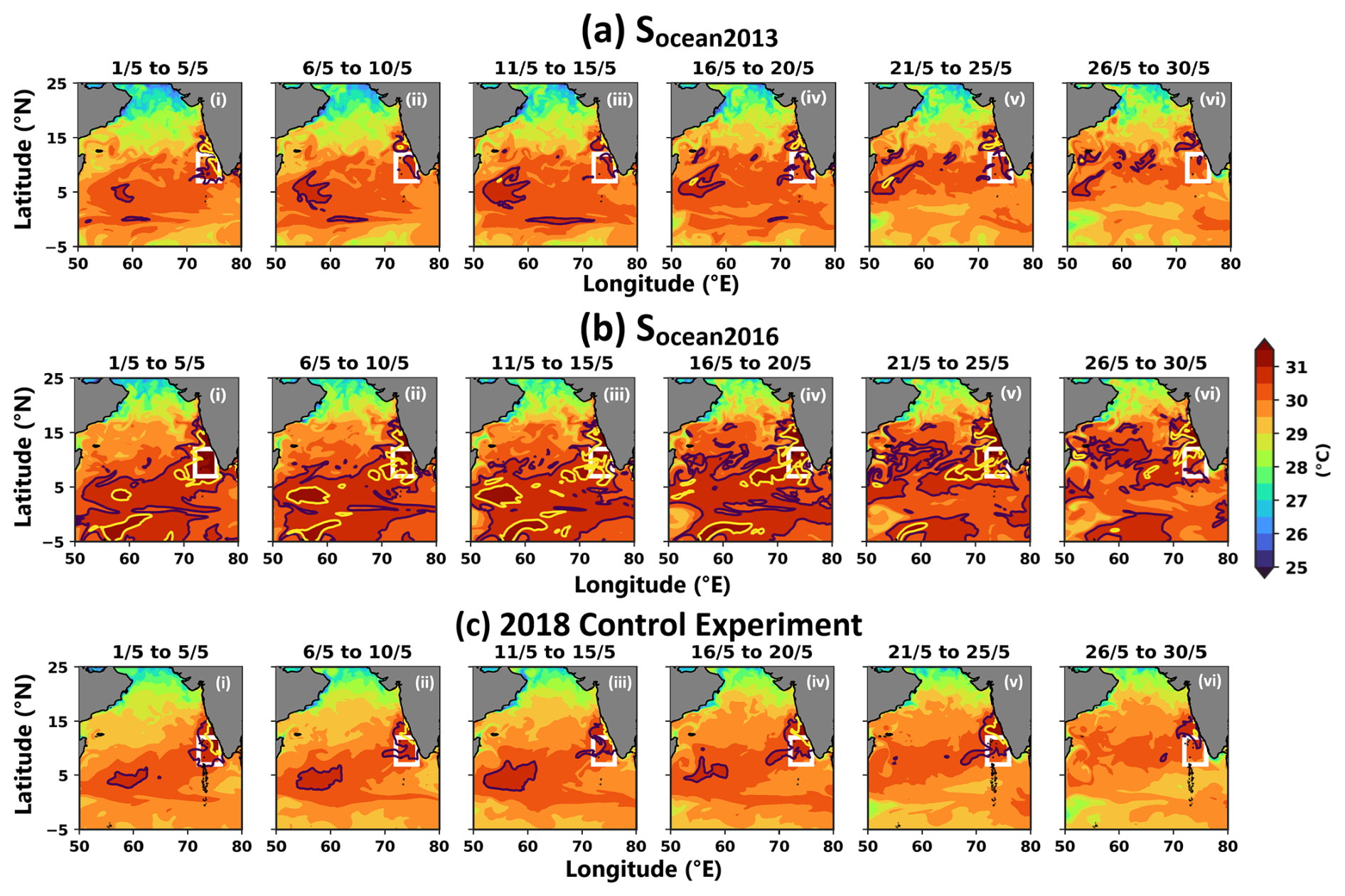
Figure 9 The 5 d average evolution of SST from 1 to 30 May for the (a) S_ocean2013, (b) S_ocean2016, and (c) 2018 control experiments. In the S_ocean2013 and S_ocean2016 experiments, the ocean's initial condition was replaced to 2013 and 2016 in the 2018 control experiment. See Table 1 for further details about the experiments. The black and yellow contours represent 30.5 and 31 °C, respectively. The days associated with mean evolution are displayed at the top of each panel. The white box is the core MWP region.

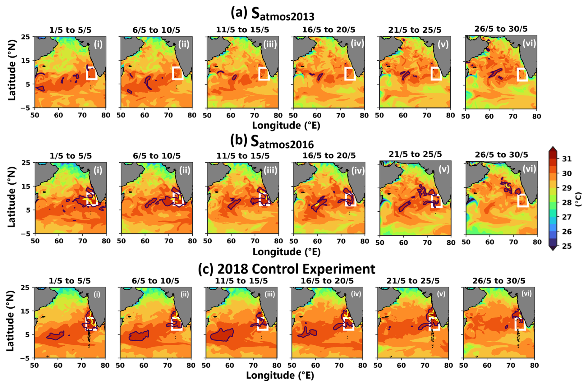
Figure 10 The 5 d average evolution of SST from 1 to 30 May for the experiment (a) S_ocean2013, (b) S_ocean2016, and (c) 2018 control experiments. In the S_ocean2013 and S_ocean2016 experiments, the atmospheric condition was replaced in 2013 and 2016 in the 2018 control experiment. See Table 1 for further details about the experiments. The black and yellow contours represent 30.5 and 31 °C, respectively. The days associated with mean evolution are displayed at the top of each panel. The white box is the core MWP region.

Later, in the S_atmos2013 experiment, the 2013 atmospheric conditions were replaced with the 2018 control experiment's atmospheric conditions. The MWP is absent in the 2013 control and S_atmos2013 experiments (Figs. 10a and 6d). Similarly, the 2016 atmospheric conditions replace those used in the 2018 control experiment, which is termed the S_atmos2016 experiment. A strong MWP was observed in the S_atmos2016 experiment (Fig. 10b), albeit with a lower intensity than in the 2016 control (Fig. 6g) and S_ocean2016 (Fig. 9b) experiment, indicating that pre-April ocean conditions were responsible for the formation of an intense MWP in the 2016 control experiment. In the S_atmos2016 and 2016 control experiments, the MWP matured on 4 May. Similarly, the S_ocean2016 and 2018 control experiments have analogous atmospheric conditions, and the MWP matures on 20 May (Fig. 9b and c). These findings suggest that the atmospheric variables determine the spatial variability in the MWP as well as the day of maturation.

The mixed-layer heat budget in the core region of the MWP (72–76° E and 7–13° N) is analyzed to allow for a better understanding of the factors contributing to its expansion and dissipation. The atmospheric conditions remain unchanged in the S_ocean2013, S_ocean2016, and 2018 control experiments. A dip in the net surface heat flux from 0.1 to −0.07 °C d⁻¹ is noticed on 8 May in these three experiments. Later, this net surface heat flux supplied to the mixed-layer temperature tendency with a maximum of 0.1 °C d⁻¹ from 15 to 18 May (Fig. 11a, d, and e), and the MWP matured on 20 May thereafter. During the dissipation phase of the MWP, the net surface heat flux had an adverse impact on the temperature tendency in S_ocean2013, S_ocean2016, and 2018 control experiments. The vertical processes also had a cooling effect on the temperature tendency, which peaked at −0.09 °C d⁻¹ on 26 May in S_ocean2013, S_ocean2016, and 2018 control experiments. Even if the MWP was not apparent in the 2013 and S_atmos2013 experiments (both of these experiments have similar atmospheric conditions), the net surface heat flux caused a gain of 0.05 °C in temperature within the mixed layer on 20 May (Fig. 11b and f). Once the MWP reached its mature day, the vertical processes and the net surface heat flux had a detrimental effect on the temperature tendency in the S_atmos2016 and 2016 control experiments (Fig. 11c and g). In all control and sensitivity experiments, the temperature tendency is negatively impacted by the vertical processes during May and June; nevertheless, the net surface heat flux is the primary driver behind the variation of the temperature tendency from the mature to the dissipation day. The horizontal advection had very minimal influence on the temperature tendency. Thus, atmospheric conditions modulate the mature and dissipation of the MWP.

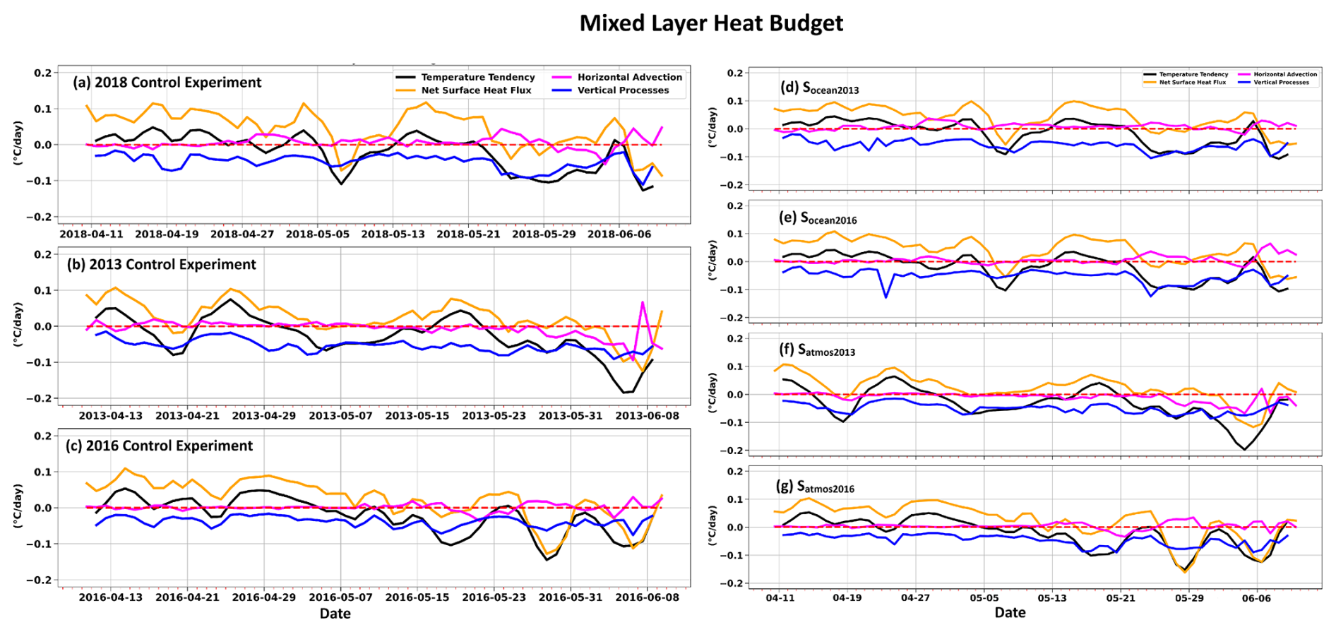
Figure 11 Area-averaged (72–76° E and 7–13° N, i.e. the white box shown in Fig. 1) mixed-layer heat budget for three control experiments – (a) 2018 control experiment, (b) 2013 control experiment, and (c) 2016 control experiment – and four sensitivity experiments – (d) S_ocean2013, (e) S_ocean2016, (f) S_atmos2013, and (g) S_atmos2016. In the sensitivity experiments, the oceanic and atmospheric conditions have been changed to various years; thus, only the day and month are kept on the x axis (d–g). For better understanding, the mixed-layer heat budget is shown from 10 April even though we consider 1 to 30 April the spin-up time.

To better assess the atmosphere's and ocean's relative contribution to the MWP intensity across different experiments, we introduced the MWP intensity index. This index is defined as follows:

$$\mathrm{MWP}\mathrm{intensity}\mathrm{index}=\mathrm{MWP}\mathrm{area}\mathrm{on}\mathrm{mature}\mathrm{day}\times \mathrm{\Delta }{T}_{\mathrm{avg}}$$

where ΔT_avg represents the average temperature change within the MWP area from its initial condition to the mature day.

In the 2016 control experiment, the MWP intensity index reached its highest value, corresponding to the warmest MWP SST and the most extensive area (Fig. 12). In contrast, the MWP was weak in the 2013 control experiment, and so was the MWP intensity index. In the S_ocean2013 experiment, where the ocean's initial and boundary conditions were modified from 2018 to 2013, the MWP intensity index decreased by 8.5 % compared to the 2018 control experiment. However, a substantial reduction of 82 % in the MWP intensity index was found when the atmospheric forcings were altered to 2013 in the S_atmos2013 experiment, highlighting the adverse effect of the atmospheric environment on the formation of the MWP.

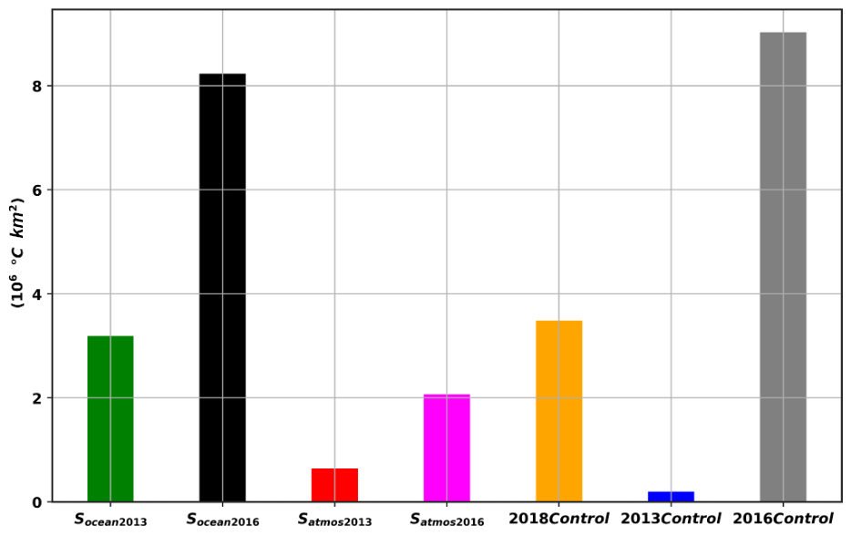
Figure 12 A comparison between the MWP intensity index in all three experiments during the respective mature-phase days in different years. In S_ocean2013, S_ocean2016, S_atmos2013, 2013 control experiment, and 2018 control experiment, the mature day was 20 May. In the S_atmos2016 and 2016 control experiments, the mature day was 4 May.

Conversely, the S_ocean2016 experiment, which replaced the 2018 oceanic initial and boundary condition with that of 2016, showed a 136 % rise in the MWP intensity index compared to the 2018 control experiment. However, when the atmospheric condition was adjusted to 2016 in the S_atmos2016 experiment, the MWP intensity index decreased by 41 %, indicating that the ocean precondition was the primary factor in the genesis of the intense MWP in 2016 and that the atmospheric condition later favored its development (Fig. 12).

3.3.2 Impact of ocean surface flux on the formation of the MWP

Once the ocean precondition was met, the atmospheric factors, including net surface heat flux, wind, and freshwater flux, played a leading role in shaping the spatial extent of the MWP. The relative importance of net thermal flux, freshwater flux, and wind on mixing is examined here using production of turbulent kinetic energy (P_TKE). Contrary to wind stirring, the P_TKE by haline and thermal buoyancy flux was of smaller magnitude in all the experiments, indicating that the wind was the driver for the mixing in SEAS in May (Fig. 13). The atmospheric conditions were similar in the 2018 control, S_ocean2013, and S_ocean2016 experiments (see Table 1 for experiment details). From 1 to 5 May, the average P_TKE caused by wind stirring was more than 8 W m⁻²; however, in the SEAS, a small wind shadow zone was formed with a very low P_TKE (Fig. 14a). Subsequently, the mixing reduced, and expansion of MWP SST was observed within this wind shadow zone in 2018 control, S_ocean2013, and S_ocean2016 experiments. A similar but much wider wind shadow zone was developed in the SEAS from 17 to 20 May, resulting in the largest MWP expansion in 2018 control, S_ocean2013, and S_ocean2016 experiments. Once the southwesterly wind strengthened, the P_TKE increased, and the ocean lost heat at the surface (Figs. 13a and 14a). In the 2013 control and S_atmos2013 experiments, atmospheric conditions were identical, and the ocean gained heat (Fig. S11b). The wind-induced P_TKE was higher in SEAS, and no such wind shadow zone was developed (Fig. 14b). Subsequently, the MWP was absent in these two experiments. In the 2016 control and S_atmos2016 experiments, the wind shadow zone was expanded over a comparatively large area from 1 to 8 May (Fig. 14c). Besides, the ocean received heat during this time in SEAS, creating favorable conditions for the development of the strong MWP (Fig. S11c).

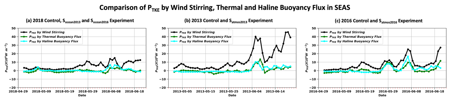
Figure 13 Comparison of the production of turbulent kinetic energy by wind, thermal, and haline buoyancy flux averaged in the SEAS (72–76° E and 7–13° N) from 1 May to 20 June. The values shown here are after multiplying by 10⁴.

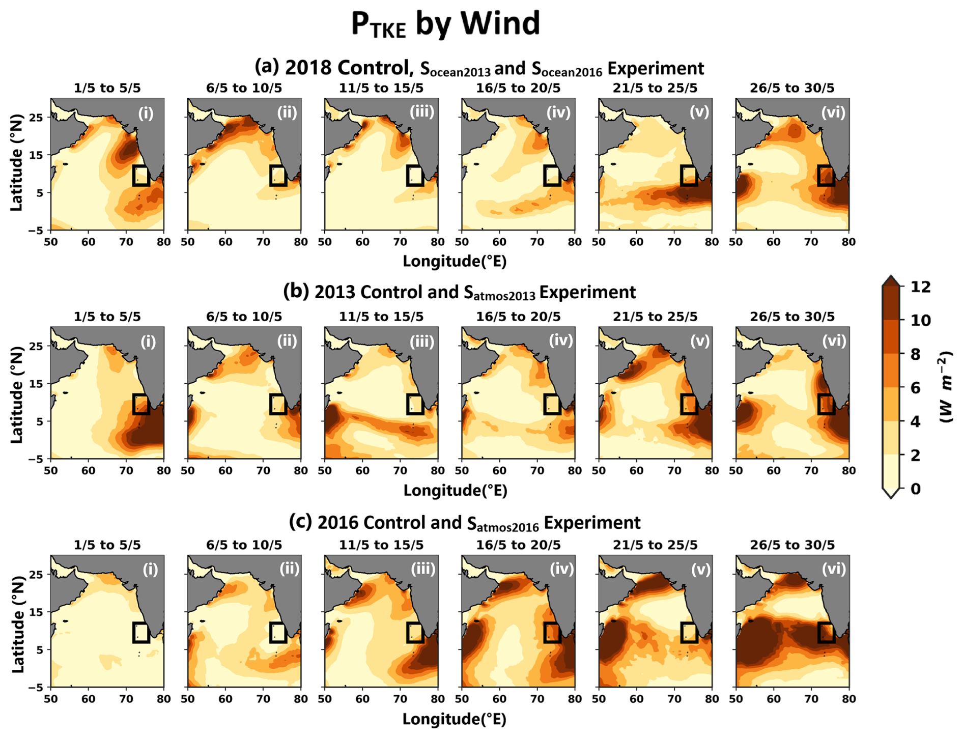
Figure 14 The 5 d average evolution of wind-induced production of turbulent kinetic energy for all control and sensitivity experiments. The fill values are shown after multiplying 10⁴. Atmospheric forcings are identical for the 2018 control, S_ocean2013, and S_ocean2016 experiments. Likewise, the wind-induced production of turbulent kinetic energy remains the same across all three experiments (a). Similarly, the wind-induced production of turbulent kinetic energy owing to thermal buoyancy flux in the 2013 control experiment and S_ocean2013 (b) and the 2016 control experiment and S_ocean2016 (c) are identical. Table 1 shows details from the sensitivity experiments. The days associated with mean evolution are listed at the top of each panel.

4 Conclusion

A coupled atmosphere–ocean numerical model has been employed to investigate the formation and evolution of the MWP in the SEAS. The model is simulated for three independent years: 2013, 2016, and 2018. The simulated results can reproduce the MWP features and showed good agreement with satellite and buoy data (Figs. 2–5 and S2–S5). The evolution of the atmospheric and ocean features near the SEAS from the mature to the dissipation day is well represented in the model. Four sensitivity experiments further elucidated the roles of oceanic and atmospheric conditions in the MWP formation. The changes in ocean initial conditions substantially impacted the magnitude of the MWP core temperature, resulting in 0.6 °C higher temperature in S_ocean2016 and 0.3 °C lower temperature in S_ocean2013 compared to the 2018 control experiment (Fig. S10d and e are compared with Fig. S10a), indicating the influence of the ocean initial condition in the MWP intensity. Analysis of the mixed-layer heat budget (Fig. 11) revealed that net surface heat flux is the primary driver of the MWP development, contributing significantly to the increase in mixed-layer temperature in the control and sensitivity experiments. It contributed more than 0.1 °C d⁻¹ to the increased temperature just before the MWP matured on the day of 2018. Vertical processes negatively affected temperature tendencies and could reach as high as −0.08 °C d⁻¹. As the moisture-rich southwesterly wind strengthened in late May to early June, it caused cloudiness, blocking the incoming shortwave radiation and the loss of latent heat flux in the SEAS (Figs. S6 and S8). Thus, the net surface heat flux, along with vertical processes, emerges as the primary driver behind the dissipation of the MWP (Fig. 11).

The atmospheric conditions remain the same in the 2018 control experiment, S_ocean2013, and S_ocean2016 experiments. Since the wind governs the MWP's advancement from mature to dissipation day by primarily controlling the net surface heat flux and the vertical processes, we have observed an identical contribution of the net surface heat flux and the vertical processes on the temperature tendency in these three experiments (Fig. 11a, d, and e). The MWP did not emerge in 2013, and when we replaced the atmospheric (ocean) condition of the 2018 control experiment with the 2013 control experiment in the S_atmos2013 (S_ocean2013) sensitivity experiment, we saw an 82 % reduction (8.5 % reduction) in MWP intensity index when compared to the 2018 control experiment. This suggested that in the weak-MWP year, although the ocean preconditions were met, the atmospheric forcing restricted the development of the MWP in SEAS. The MWP intensity index also revealed that the shuffling of the atmospheric forcings and oceanic initial conditions of the strong-MWP year to the year of the MWP whose intensity was identical to climatology (S_atmos2016 and S_ocean2016 experiments) resulted in a substantial decrease of 41 % and increase of 136 % in the MWP intensity index (Fig. 12), which demonstrated that in the strong-MWP year, the pre-April ocean condition played a considerable role in the development of the MWP in May, which was further supported by the prevailing atmospheric conditions.

Later, P_TKE was computed to study the mixing in the SEAS. The influence of wind-induced P_TKE on mixing surpassed that of P_TKE caused by thermal and haline buoyancy flux (Fig. 13). Further, a wind shadow zone with a lower P_TKE was witnessed in SEAS. The MWP advanced within this zone (Fig. 14). However, this shadow zone was absent in experiments such as the 2013 control and S_atmos2013 experiments. The MWP did not develop in these two experiments, although the ocean preconditions were met, indicating that the wind shadow zone was a key factor in the MWP's advancement within the SEAS.

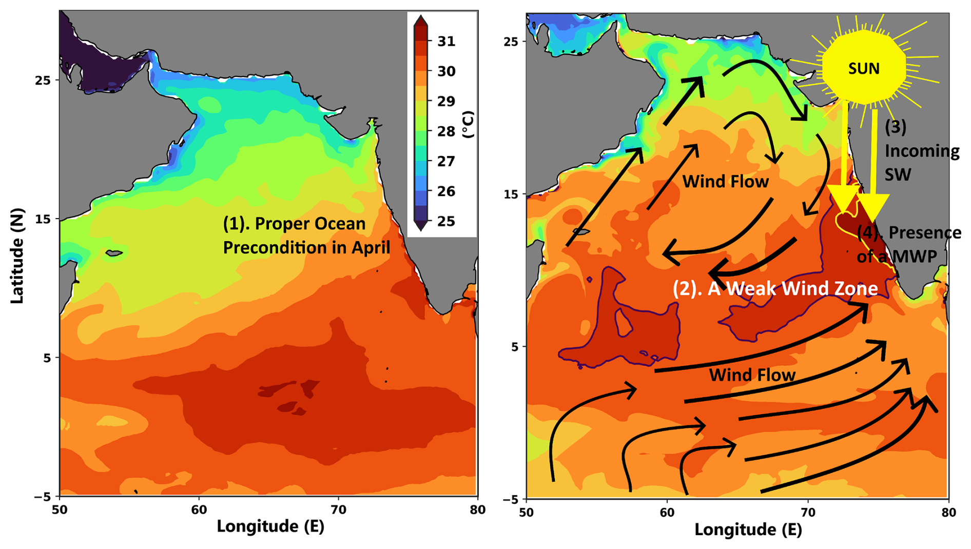
Figure 15 Schematic of the atmospheric and oceanic conditions associated with the formation of the MWP. The numbering denotes the importance of that process in the formation of the MWP. For instance, the ocean precondition (1) is the first requirement for MWP's genesis. Later, a weak wind zone (2) with less mixing traps the incoming shortwave radiation (3) in SEAS, which results in the formation of the MWP (4). Both panels have the same color bar levels. The black and yellow contours represent 30.5 and 31 °C, respectively.

In conclusion, once the ocean conditions before April have laid the foundation (1 in Fig. 15), the prevailing atmospheric conditions develop a weak wind zone in SEAS in May (2 in Fig. 15), and the incoming shortwave radiation flux under the clear sky is trapped within this zone (3 in Fig. 15). Subsequently, the MWP advances inside this area. Thus, a strong MWP can only occur in SEAS if all of these requirements are met (Fig. 15). After the MWP matures, the strong southwesterly wind in SEAS creates cloudiness and increases P_TKE, which blocks incoming shortwave radiation and causes the MWP to dissipate as the net surface heat flux decreases. The current study seeks to understand the impact of the ocean and atmosphere on the MWP during its mature phase and the factors that contribute to its dissipation. We concluded that atmospheric conditions such as wind influence the spatial variability in the MWP. Nonetheless, ocean preconditions before April have a substantial effect on MWP strength. Given the importance of ocean preconditioning in MWP genesis, it would be interesting to analyze the warming chronology of the southeastern Arabian Sea before the formation of a strong MWP, such as in 2016, which serves as the future scope of the current study. Besides, the wind shadow zone appears during a year with high MWP SST, and we hypothesize that this shadow zone and the resulting increase in MWP SST is linked with the onset of the Indian summer monsoon. However, further investigation is necessary, which is beyond the scope of the present study.