Dual-tracer constraints on the inverse Gaussian transit time distribution improve the estimation of water mass ages and their temporal trends in the tropical thermocline

Quantifying the mean state and temporal change of seawater age is crucial for understanding the role of ocean circulation and its change in the climate system. One commonly used technique to estimate the water age is the inverse Gaussian transit time distribution method (IG-TTD), which applies measurements of transient abiotic tracers like chlorofluorocarbon 12 (CFC-12). Here, we use an Earth system model to evaluate how accurately the IG-TTD method infers the mean state and temporal change of true water age from 1981 to 2015 in the tropical thermocline (on isopycnal layer σ₀=25.5 kg m⁻³). To this end, we compared the mean age of IG-TTD (Γ) derived from simulated CFC-12 with the model “truth”, the simulated ideal age. Results show that Γ underestimates the ideal age of 46.0 years by up to 50 %. We suggest that this discrepancy can be attributed to imperfect assumptions about the shapes of the transit time distribution of water parcels in the tropics and the short atmospheric history of CFC-12. Moreover, when only one transient tracer (CFC-12) is available, temporal trends in Γ might be an unreliable indicator and, due to uncertainties in the mixing ratio, may even be of opposite sign to temporal trends in the ideal age. The disparity between Γ and ideal age temporal trends can be significantly reduced by incorporating an additional abiotic tracer with a different temporal evolution, which we show by constraining Γ with sulfur hexafluoride (SF₆) in addition to CFC-12.

1 Introduction

Ocean ventilation, i.e., the processes transporting surface water and its associated properties including heat, nutrients, oxygen, and other gases such as carbon dioxide (CO₂) to the ocean interior, is of great importance to marine ecosystems and the climate system. Under current transient climate conditions, ventilation slows down the increase in surface air temperature and the rise in atmospheric CO₂ by transporting excessive heat and CO₂ absorbed at the ocean surface into the ocean interior (e.g., Waugh et al., 2004; Sabine et al., 2004; Banks and Gregory, 2006; Sabine and Tanhua, 2010; Khatiwala et al., 2013). Moreover, ventilation supplies oxygen-rich surface water into the aphotic (light-deprived) interior of the ocean, where oxygenic photosynthesis does not occur, thereby enabling aerobic organisms to thrive and reproduce in the deep ocean. This is particularly important as many of these organisms, including fish, have significant ecological and economic value, particularly as a global food supply.

One method to determine the ventilation strength is by estimating the passage time (the time elapsed since a water parcel was last in contact with the atmosphere, i.e., water age). This property cannot be measured directly in the ocean, but it can be diagnosed from measurements of transient abiotic tracers (e.g., Jenkins, 1980; Weiss et al., 1985), such as sulfur hexafluoride (SF₆) and chlorofluorocarbons (CFCs, e.g., CFC-11 and CFC-12), which are purely non-natural and have well-defined source functions in the atmosphere (Bullister, 2015). The concept of water mass age has been widely used to estimate the storage of anthropogenic CO₂ in the ocean interior (Gruber, 1998; Waugh et al., 2004; Khatiwala et al., 2009) and to quantify rates of biogeochemical processes, such as oxygen utilization rates (OURs; Jenkins, 1987; Sonnerup et al., 2013, 2015; Koeve and Kähler, 2016; Guo et al., 2023). Various techniques have been developed to derive water age from these tracers, with the transit time distribution (TTD) method being one of the well-established approaches (Haine and Hall, 2002; Waugh et al., 2003). In contrast to alternative methods like the CFC-12 tracer concentration age (Doney and Bullister, 1992), the TTD method accounts for the fact that water parcels in the deep ocean comprise fluid elements with different origins and pathways, thus representing a spectrum of transit times from the ocean surface to the interior location of consideration. One common assumption with respect to the spectrum of individual transit times is the inverse Gaussian, which results from one-dimensional transport and mixing. We, and other previous studies, referred to this TTD as IG-TTD (see details in Sect. 3).

Previous studies using the IG-TTD approach have shown evidence of regional changes in ocean ventilation due to climate change (Waugh et al., 2013; Jeansson et al., 2023). In the Southern Ocean, the IG-TTD mean age of the Subantarctic Mode Water (SAMW) has decreased and the IG-TTD mean age of Circumpolar Deep Water (CDW) has increased over the past decades due to the strengthening and poleward shift in the westerly winds (Waugh et al., 2013). In the Nordic Seas, Jeansson et al. (2023) found overall enhanced ventilation in the upper 1500 m from the 1990s to the 2010s and reduced ventilation in the deeper waters. Monitoring and understanding these changes is crucial to assess their consequences on ecosystems and predict future responses to climate change.

However, the IG-TTD studies mentioned above usually assume (i) a prescribed constant ratio of mixing and advective transport in the ocean ($\mathrm{\Delta }/\mathrm{\Gamma }$, i.e., the ratio between the width, Δ, and mean, Γ, of the age spectrum) and (ii) 100 % saturation of transient tracers during water mass formation. Uncertainties regarding the validity of these assumptions can induce uncertainties in the TTD-derived estimates of ventilation and its temporal changes under a changing climate. Even though the limitations of the IG-TTD technique related to the above assumptions have been studied intensively over the past decade (e.g., Peacock et al., 2005; Shao et al., 2013, 2016; He et al., 2018; Raimondi et al., 2021, 2023), most of these studies have only focused on the subtropical gyres, whereas very few have focused on the tropics (see details in Sect. 3). Moreover, available observations of CFC-12 and SF₆ in the tropics (Lauvset et al., 2022) can potentially contribute to our understanding of the ocean's ventilation state and its temporal change in this region. Therefore, we evaluate the IG-TTD technique in the tropical ocean in this study.

While the true (ideal) age in the real ocean can not be measured directly and is, hence, not known, numerical ocean models provide the possibility to simulate this property as an explicit tracer, along with simulated transient tracers such as CFC-12 and SF₆. Therefore, comparing the IG-TTD ages derived from the latter with simulated ideal age provides the possibility to investigate the implication of the assumptions inherent in the IG-TTD method for age estimates. Here, we employ an Earth system model (ESM) to investigate whether and the extent to which the mean age computed from the IG-TTD method is able to represent the ideal age and the temporal changes in the ideal age under global warming in the upper tropical thermocline. Section 2 describes the model, the Flexible Ocean and Climate Infrastructure (FOCI), and the experimental setup. In Sect. 3, the IG-TTD concept and the commonly used assumptions are introduced. Section 4 shows IG-TTD biases and relates these to the applied assumptions. We discuss the IG-TTD application's possible limitations and recommendations for possible improvements in Sect. 5.

2 Model description

The Flexible Ocean and Climate Infrastructure (FOCI; Matthes et al., 2020) ESM is used in this study. FOCI uses the latest release of the European Centre Hamburg general circulation model (ECHAM6.3) with a nominal resolution of 1.8 × 1.8° as the atmospheric component. The Nucleus for European Modelling of the Ocean (NEMO3.6; Madec and the NEMO System Team, 2016) is used for its ocean circulation component and is coupled with the Model of Oceanic Pelagic Stoichiometry (MOPS) ocean biogeochemistry model (Kriest and Oschlies, 2015; Chien et al., 2022). The Louvain-la-Neuve sea Ice Model (LIM2) is the sea ice module, and the Jena Scheme for Biosphere–Atmosphere Coupling in Hamburg (JSBACH) is the land surface component. The ocean, atmosphere, and land components are coupled via the OASIS3-MCT coupler (Valcke, 2013).

CFC-12 and SF₆ are simulated as passive tracers in NEMO3.6 with a 0.5 × 0.5° global tripolar grid. The model is vertically discretized on 46 geopotential levels with thickness ranging from 6 m at the surface to 250 m in the deep ocean. Two-step flux-corrected transport, namely the total variance dissipation (TVD) scheme (Zalesak, 1979), is used for tracer advection to ensure positive definite values. Tracer diffusion is aligned along isopycnals, with diffusivity set as 600 m² s⁻¹. In the upper ocean, the mixed-layer depth is diagnosed by turbulent kinetic energy (TKE) (Blanke and Delecluse, 1993) and vertical mixing is increased for unstable water columns, representing convection in regions of deep and bottom water formation. The relatively coarse resolution does not allow for the resolution of mesoscale eddies; therefore, the eddy-induced transport is parameterized using the Gent and Mcwilliams (1990) scheme.

An additional tracer, the idealized age tracer, is also included in the ocean component. The idealized age tracer works like a “clock”, set to zero at the sea surface and elapsing at a rate of 1 d d⁻¹ below the surface layer (Thiele and Sarmiento, 1990; England, 1995; Koeve et al., 2015). In other words, the ideal age is the mean age of water parcels that contribute to a grid point in the model but without the constraint of a particular shape (i.e., IG) of the TTD. In this paper, the ideal age serves as a “model truth” of the seawater age.

2.1 Experimental setup

Details of the model setup have been described by Chien et al. (2022); thus, we provide only a brief description here. Firstly, the “physics-only” model (FOCI) was spun up for 1500 years under constant preindustrial (PI) forcing conditions (e.g., 280 ppm CO₂ and seasonally prescribed aerosol concentrations; Matthes et al., 2020). The physics-only model was initialized from rest with temperature and salinity fields from version 2.1 of the Polar science center Hydrographic Climatology (PHC2.1; Steele et al., 2001) and sea ice from an uncoupled ocean-only hindcast simulation (“WEAK 05” experiment; Behrens et al., 2013). After the 1500 years of physical spin-up, the coupled ESM including ocean biogeochemistry was further integrated for 500 years under PI forcing conditions, followed by a 250-year (drift) period with zero CO₂ emissions during which atmospheric CO₂ concentrations were computed prognostically. The biogeochemical tracers phosphate, nitrate, and oxygen were initialized using the World Ocean Atlas 2013 (WOA2013; Garcia et al., 2013a, b) dataset, and preindustrial dissolved inorganic carbon and alkalinity were initialized by GLODAPv2.2016b (Lauvset et al., 2016). The ideal age followed the same spin-up strategy as the biogeochemical tracers but was initialized with zeros everywhere in the ocean. Because an age tracer starting from age zero requires up to several thousand years to reach an equilibrium state in the ocean (Wunsch and Heimbach, 2008), the idealized age tracer was still drifting significantly after the 750-year spin-up for fully coupled FOCI, albeit mainly in the deep ocean. At our focus regions in the upper thermocline, the drift of the idealized age tracer was negligible, as detailed in Sect. 4.1.

Branching off from the spin-up state, we performed the historical and preindustrial experiments following the Coupled Model Intercomparison Project 6 (CMIP6) protocol for the emission-driven experiments (Eyring et al., 2016). The historical (equivalent to “esm-hist” in CMIP6) and preindustrial control (equivalent to “esm-piControl” in CMIP6) simulations were each carried out for 165 years (1850–2014). The esm-hist simulation uses historical CO₂ emissions and prescribed historical time series of non-CO₂ greenhouse gas (e.g., methane and nitrous oxide) concentrations and land use (Meinshausen et al., 2017). The esm-piControl simulation is integrated with zero emissions of CO₂ and a prescribed constant non-CO₂ greenhouse gas concentration, and it employs land use conditions that are representative of the Earth around the year 1850 (Eyring et al., 2016).

Implementation of the transient tracers follows the CMIP6 protocol (Orr et al., 2017). Boundary conditions for atmospheric transient tracers are prescribed for the time period from 1936 to 2015 with exactly the same time evolution in the esm-piControl and esm-hist runs (Fig. S1 in the Supplement; Bullister, 2015), assuming slightly differing tropospheric surface mixing ratios of CFC-12 and SF₆ for the Northern Hemisphere and Southern Hemisphere, respectively. Air–sea gas exchange is computed following Eqs. (1)–(2):

$$\begin{array}{}\text{(1)}& {\displaystyle }{\mathrm{flux}}_{\mathrm{a}-\mathrm{o}}=(\mathrm{1}-f_{\mathrm{ice}})\cdot k_{\mathrm{w}}\cdot (C_{\mathrm{equilibrium}}-C_{\mathrm{o}}),\text{(2)}& {\displaystyle }{k}_{\mathrm{w}}=a\cdot U^{\mathrm{2}}\cdot {\left({\displaystyle \frac{\mathit{Sc}}{\mathrm{660}}}\right)}^{\mathrm{2}}.\end{array}$$

Here positive flux_a−o is the flux from the atmosphere to the ocean; f_ice represents the fraction of sea ice in the respective grid cell; C_equilibrium is the saturation concentration of CFC-12 and SF₆, determined using sea surface temperature, salinity, and the corresponding atmospheric partial pressure of tracers (Warner and Weiss, 1985; Bullister et al., 2002; Bullister, 2015); and C_o is the simulated concentration of transient tracers in seawater at the ocean surface. The gas transfer velocity (k_w) is determined by a quadratic function of 10 m wind speed (U) and by using the revised Schmidt number (Sc) of individual transient tracers (Wanninkhof, 1992, 2014). The value of the constant a is 0.251 (cm h⁻¹) (m s⁻¹)⁻² (Wanninkhof, 2014)

2.2 Model validation

The skill of FOCI with respect to representing the real ocean ventilation patterns in the thermocline and intermediate waters (${\mathit{\sigma }}_{\mathrm{0}}=\mathrm{25.5}\pm \mathrm{0.5}$ kg m⁻³) is evaluated by comparing the mixing ratio of CFC-12 (in units of part per trillion – ppt) in the model ocean and the real ocean. We derived the mixing ratio by dividing the CFC-12 concentration by temperature- and salinity-dependent solubility (Warner and Weiss, 1985). For the real ocean, we used the Global Ocean Data Analysis Project products (GLODAPv2.2022; https://www.ncei.noaa.gov/access/ocean-carbon-acidification-data-system/oceans/GLODAPv2_2022/, last access: 9 February 2023, Lauvset et al., 2022), which provide temperature, salinity, and concentrations of transient tracers and other biogeochemical tracers. For model simulations, we convert the unit of model output of CFC-12 concentration from picomoles per cubic meter (pmol m⁻³) to picomoles per kilogram (pmol kg⁻¹; unit in the observational product) by dividing by 1025 kg m⁻³, i.e., using a constant density of seawater. Moreover, we subsampled the monthly mean model outputs according to when and where the data were measured.

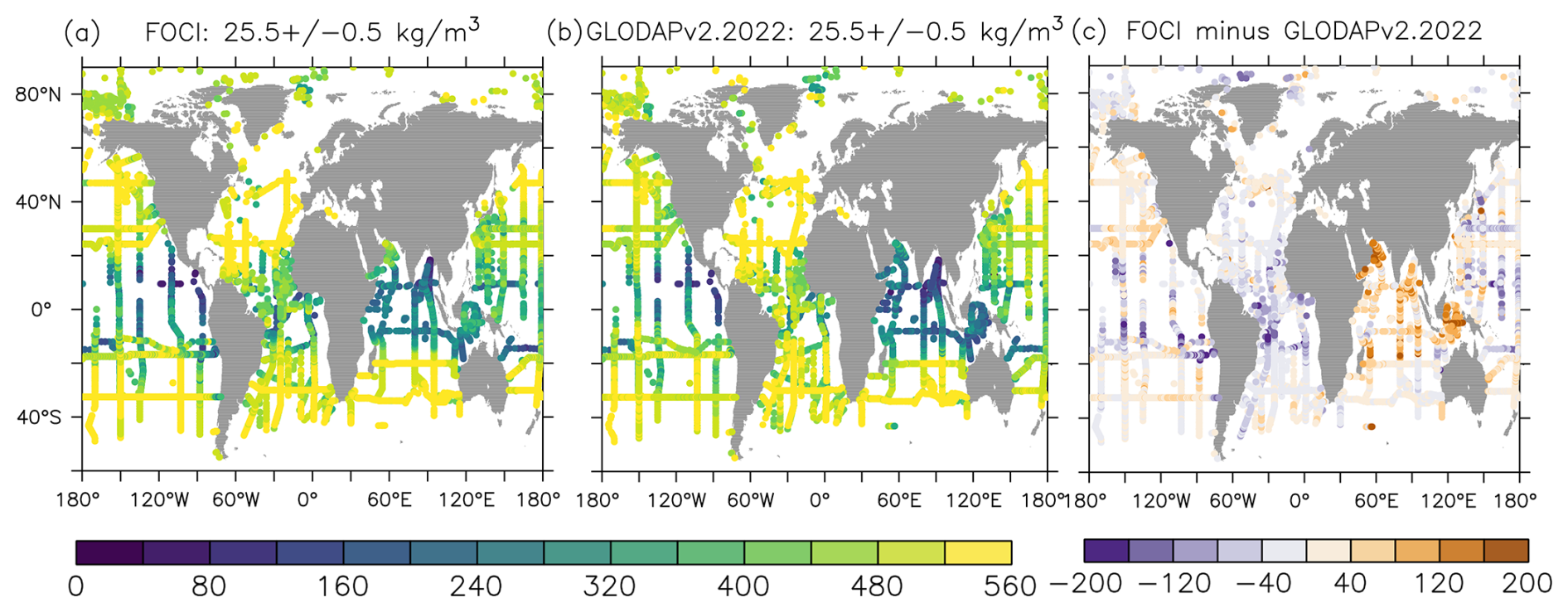
Figure 1 Distribution of (a) the subsampled simulated CFC-12, (b) the observed CFC-12 mixing ratio, and (c) their difference on the isopycnal layer ${\mathit{\sigma }}_{\mathrm{0}}=\mathrm{25.5}\pm \mathrm{0.5}$ kg m⁻³ (in units of parts per trillion – ppt).

The broad agreement on the distribution of CFC-12 mixing ratios between the model simulation and observations in the thermocline and intermediate waters suggests that the model represents the ventilation of the upper ocean reasonably well (Fig. 1). The pattern correlation coefficient between our subsampled model outputs and observation is 0.868, and the bias is −2.84 ppt (model minus observation, equivalent of −0.59 % of observation). Both simulations and observations show a high partial pressure of CFC-12 in the subtropics (and further north in the Atlantic Ocean) and a low partial pressure in the tropics, especially in the eastern North Pacific Ocean where direct contact with the atmosphere is restricted by ocean circulation. This region is known as the ocean “shadow zone” of the ventilated thermocline (Luyten et al., 1983). Relatively high negative biases occur in the tropical South Atlantic and northwest tropical Pacific, which suggest models' underestimation of ventilation in these regions.

3 IG-TTD approach

TTD is a distribution of the transit times of water masses from the ocean surface to the interior considering a combination of advective and diffusive transport pathways (Haine and Hall, 2002; Waugh et al., 2003). In brief, the concentration of any passive tracer, c(r,t), at location r and time t can be related to its surface history and its transit time distribution as follows:

$$\begin{array}{}\text{(3)}& c(\mathit{r},t)=\underset{\mathrm{0}}{\overset{\propto }{\int }}{c}_{\mathrm{0}}(t-\mathit{\xi })G(\mathit{r},\mathit{\xi })\mathrm{d}\mathit{\xi },\end{array}$$

where c₀(t−ξ) is the history of the tracer concentration at the surface ocean ξ years before the time of observation t. For CFC-12 and SF6 used in this study, their atmospheric history has been observed from 1936 to 2015 (Bullister, 2015), which provides the boundary condition c₀. G(r,ξ) is the transit time distribution at location r. Assuming that the TTD takes the shape of an inverse Gaussian (IG) function (Waugh et al., 2003), G(r,ξ) can be written as follows:

$$\begin{array}{}\text{(4)}& G(\mathit{r},\mathit{\xi })=\sqrt{{\displaystyle \frac{{\mathrm{\Gamma }}^{\mathrm{3}}}{\mathrm{4}\mathit{\pi }{\mathrm{\Delta }}^{\mathrm{2}}{\mathit{\xi }}^{\mathrm{3}}}}}\exp \left({\displaystyle \frac{-\mathrm{\Gamma }(\mathit{\xi }-\mathrm{\Gamma }{)}^{\mathrm{2}}}{\mathrm{4}\mathrm{\Delta }\mathit{\xi }}}\right).\end{array}$$

The shape of G(r,ξ) is determined by the mean age (Γ) and the variance of the distribution of age scales, i.e., “age spectral width” (Δ), which are expressed as follows:

$$\begin{array}{}\text{(5)}& {\displaystyle }\mathrm{\Gamma }=\underset{\mathrm{0}}{\overset{\propto }{\int }}\mathit{\xi }G(\mathit{r},\mathit{\xi })\mathrm{d}\mathit{\xi },\text{(6)}& {\displaystyle }\mathrm{\Delta }={\displaystyle \frac{\mathrm{1}}{\mathrm{2}}}\underset{\mathrm{0}}{\overset{\propto }{\int }}(\mathit{\xi }-\mathrm{\Gamma }{)}^{\mathrm{2}}G(\mathit{r},\mathit{\xi })\mathrm{d}\mathit{\xi }.\end{array}$$

Assuming the inverse Gaussian form (Eq. 4) with the two unknown parameters Γ and Δ will imply an unlimited number of (Γ, Δ) pairs, given a measured interior concentration of a single transient tracer. Making assumptions with respect to the Δ $/$ Γ ratio will reduce the number of unknowns to 1 and, thereby, allows the estimation of both Γ and Δ from the measurement of a single transient tracer. The Δ $/$ Γ ratio reflects the relative importance of diffusive and advective processes for the ventilated water mass (Waugh et al., 2003). A Δ $/$ Γ of 0 represents a purely advective flow, whereas a Δ $/$ Γ>1 indicates a predominantly diffusive transport. The Δ $/$ Γ ratio can, theoretically, be constrained by applying two tracers with different input functions coming from their atmospheric time histories (e.g., Waugh et al., 2003; Sonnerup et al., 2015). A tracer pair measured and used for this purpose is CFC-12–SF₆ (e.g., Tanhua et al., 2008; Stöven et al., 2016). Theoretically, the Δ $/$ Γ ratio can vary over a large range in nature. However, when Δ $/$ Γ exceeds 1.8, the water age cannot be well constrained by the CFC-12–SF₆ pair (Waugh et al., 2003; Stöven et al., 2015). Effectively, the search range of Δ $/$ Γ is therefore restricted to be smaller than 1.8, which is also the case in this study.

Additional uncertainty in the TTD-based mean age arises from the assumption of constant (usually 100 %) saturation of transient tracers at the time of water mass formation (Shao et al., 2013; Stöven et al., 2015; He et al., 2018; Raimondi et al., 2021; Jeansson et al., 2023; Raimondi et al., 2023). A 100 % saturation assumption is not generally realistic in deep-water formation regions, and it causes the tracer-derived age to be older than with a more realistic, undersaturated boundary condition (Shao et al., 2013; He et al., 2018; Raimondi et al., 2021). Moreover, the saturation levels of transient tracers in high-latitude regions increased from 1940 onwards (He et al., 2018; Raimondi et al., 2021). These changes include variations in the mixed-layer depth, growth rates of atmospheric partial pressure, and warming-driven adjustment in solubility (Shao et al., 2013). Considering such imperfect saturation levels, TTD-derived water ages range from being 0.5 years younger in the upper ocean to 15 years younger in the deep ocean, compared to estimates based on a constant 100 % saturation level (He et al., 2018).

Here, we calculate the IG-TTD-based mean age from simulated CFC-12, implementing (1) a range of globally homogeneous Δ $/$ Γ values (0.8, 1.0, 1.2, and 1.4) (Sect. 4.2), (2) regionally and temporally varying Δ $/$ Γ values constrained by simulated CFC-12 and SF₆ (Sect. 4.3), and (3) different saturation level assumptions (100 % saturation and time-varying saturation) (Sect. 4.4). Instead of choosing one specific point in time, we focus on the time series of Γ for the period from 1981 to 2015 when CFC-12 concentrations were intensively measured in the real ocean. We target the isopycnal layer encompassing the thermocline and intermediate waters (σ₀=25.5 kg m⁻³ at about 40–450 m depth; Fig. 2c), which is specifically of interest due to the oxygen minimum zones located in this density range. Moreover, the ideal age on this layer is younger than 200 years, which is in the range where CFC-12-based IG-TTD is supposed to be functional with its limited (around 80 years) time history (Sulpis et al., 2021). We use the ideal age as a reference measure to evaluate whether Γ derived from a CFC-12-informed IG-TTD is able to adequately reflect the ventilation processes and their temporal changes.

4 Results

4.1 Idealized age tracer and apparent oxygen utilization

The simulated preindustrial ventilation pattern via the ideal age on the σ₀=25.5 kg m⁻³ isopycnal is depicted in Fig. 2a. From the outcrops at midlatitudes to the tropics, the ideal age increases from 1 to 80 years. Upwelling, which brings older water from the ocean interior to the upper ocean, might also contribute to elevated ages near the Equator. The oldest waters on the σ₀=25.5 kg m⁻³ isopycnal, with ages of around 150 years, appear in the eastern North Pacific Ocean where direct contact with the atmosphere is restricted by ocean circulation. Apparent oxygen utilization (AOU; i.e., the difference between the saturated oxygen concentration and the measured oxygen concentration) shows a similar spatial pattern to the ideal age (i.e., the AOU is high in old waters and vice versa) (Fig. 2b). However, low-AOU (i.e., oxygen-rich) waters are found in the tropical Atlantic Ocean, where the depth of the isopycnal layer is shallower than 80 m; hence, these low-AOU waters are observed within a depth range where oxygen production via photosynthesis may occur. Importantly, the global averages of the ideal age and AOU (Fig. 2d, e) show very little drift in esm-piControl simulations ($-\mathrm{0.016}\pm \mathrm{0.012}$ yr yr⁻¹ and $-\mathrm{0.030}\pm \mathrm{0.031}$ mmol m⁻³ yr⁻¹, respectively); i.e., the drift of the ideal age and AOU is negligible.

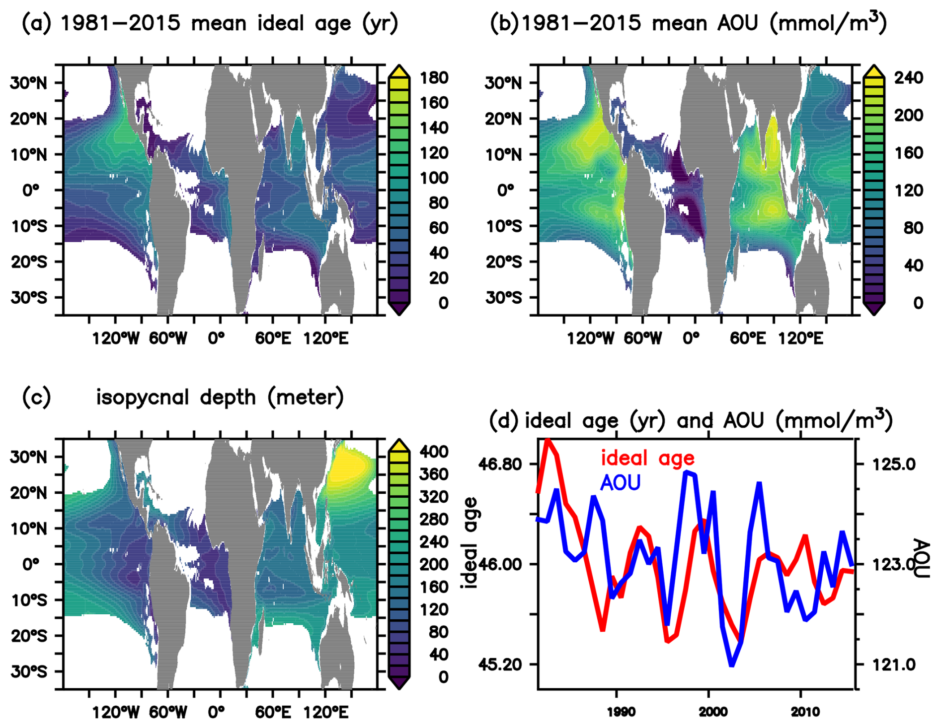
Figure 2 Distribution of the (a) ideal age (in years), (b) apparent oxygen utilization (AOU, in mmol m⁻³), and (c) depth (in meters) averaged from 1981 to 2015 at isopycnal layer σ₀=25.5 kg m⁻³ in the esm-piControl simulations. Waters shallower than the local winter mixing depth have been excluded. Panel (d) presents the temporal evolution of the ideal age (red line, left y axis) and AOU (blue line, right y axis) averaged at the isopycnal layer σ₀=25.5 kg m⁻³ in the esm-piControl simulation.

4.2 IG-TTD with spatially homogenous Δ $/$ Γ assumptions in the esm-piControl simulations

Due to the lack of SF₆ measurements before 1996 (Lauvset et al., 2022) and deliberate tracer release experiments that injected SF₆ into the deep ocean and the subsequent spreading of this SF₆ in parts of the ocean (e.g., the Nordic Seas; Watson et al., 1999; Tanhua et al., 2005; Jeansson et al., 2009), only CFC-12 is available for the IG-TTD calculation for certain regions; therefore, fixed, spatially homogeneous Δ $/$ Γ ratios are often assumed when computing the IG-TTD (commonly Δ $/$ Γ = 1±0.2; e.g., Waugh et al., 2004; Jeansson et al., 2023). Here, we evaluate the uncertainties in IG-TTD arising from different Δ $/$ Γ value assumptions (i.e., 0.8, 1.0, 1.2, and 1.4).

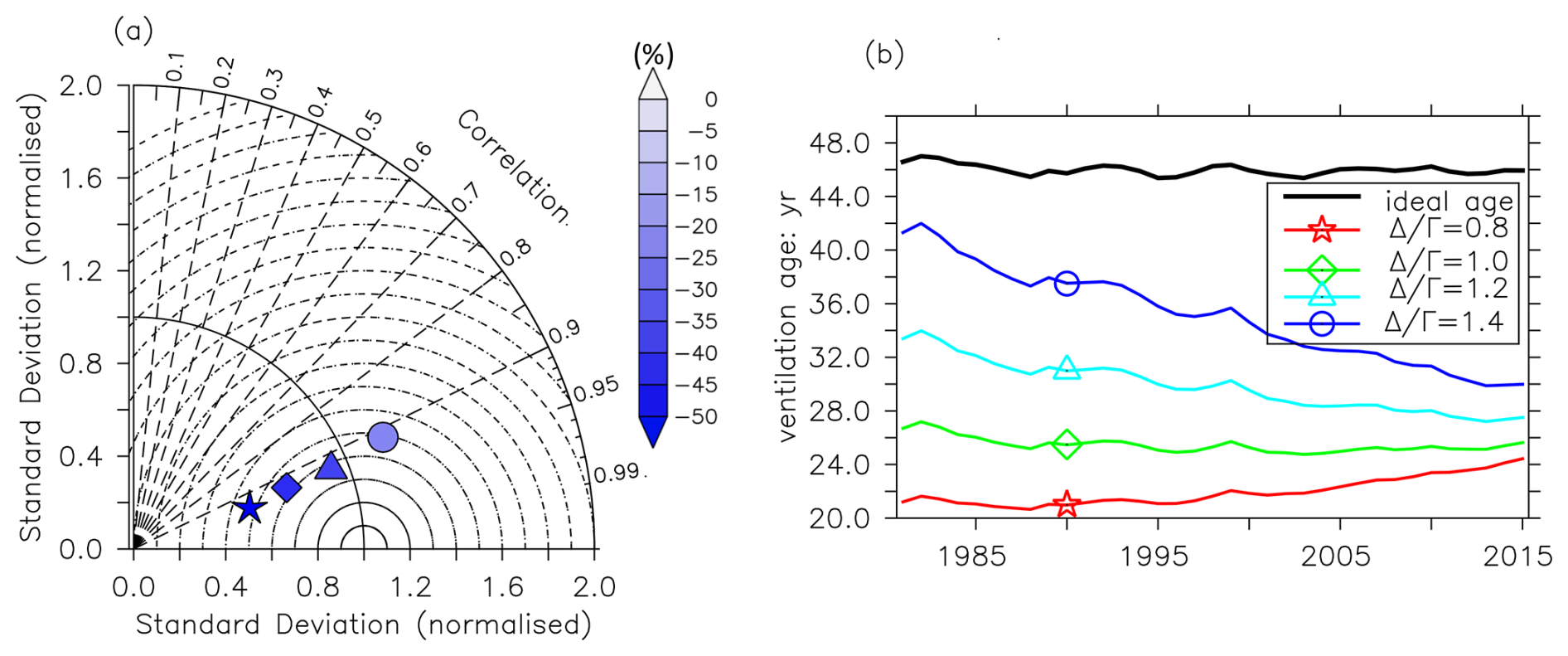
Figure 3 For the preindustrial control run, panel (a) presents the Taylor diagram between the mean age of IG-TTD averaged over 1981–2015 and the ideal age (as a reference) at isopycnal layer σ₀=25.5 kg m⁻³; the color bar on the right provides the bias (in percent). The star, diamond, triangle, and circle markers indicate that respective Δ $/$ Γ values of 0.8, 1.0, 1.2, and 1.4 were applied in the IG-TTD calculation. Panel (b) shows the globally averaged ideal age (black) and the mean age with a Δ $/$ Γ value of 0.8 (red), 1.0 (green), 1.2 (cyan), and 1.4 (blue) from 1981 to 2015.

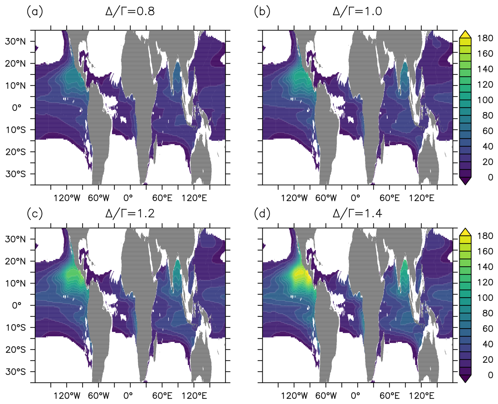
Figure 4 Panels (a), (b), (c), and (d) show the mean age of IG-TTD (Γ) averaged over 1981–2015 in the preindustrial control simulation at σ₀=25.5 kg m⁻³ with respective Δ $/$ Γ values of 0.8, 1.0, 1.2, and 1.4. The Γ value calculated here is derived from the CFC-12 in the esm-piControl simulation with a 100 % saturation state assumption.

In our esm-piControl simulation, the global mean Γ inferred from CFC-12 is consistently smaller than the ideal age on the σ₀=25.5 kg m⁻³ isopycnal, regardless of the Δ $/$ Γ assumption (Fig. 3b, Table S1). However, the difference between Γ and the ideal ages varies with different Δ $/$ Γ values. Assuming a low Δ $/$ Γ value (0.8), the horizontally averaged Γ value (22.0±2.0 years) is only 48 % of the respective ideal age value (46.0±0.8 years). This suggests that the ventilation strength in the upper thermocline is overestimated by the IG-TTD approach with this assumption. On the other hand, when assuming a higher Δ $/$ Γ value (1.4), i.e., a more diffusion-dominated transport, the mean Γ becomes larger (35.1±6.9 years), but it is still significantly smaller than the ideal age. It is also noteworthy that, besides the old waters in the northeast tropical Pacific and the Bay of Bengal with Δ $/$ Γ ratios above 1.0, the mean age of IG-TTD always underestimates the ideal age (Fig. S2). Moreover, the relative difference between the ideal age and the mean age is slightly higher in young waters.

The pattern of 1981–2015 time-averaged Γ generally agrees with the distribution of the ideal age on σ₀=25.5 kg m⁻³, i.e., a low age in subtropical regions and a high age in tropical areas (Fig. 4). For all Δ $/$ Γ assumptions, the correlation coefficient between Γ and the ideal age is above 0.9 globally. However, the spatial variability in Γ substantially differs from the simulated ideal age and is sensitive to the assumed Δ $/$ Γ (Fig. 3a). More precisely, the spatial variance in Γ increases with a higher Δ $/$ Γ, with 1.2 being the most representative of the spatial variation in the ideal age.

The CFC-12-derived Γ value shows temporal trends from 1981 to 2015 at σ₀=25.5 kg m⁻³ in our esm-piControl simulations. Such trends also depend on the assumed Δ $/$ Γ (Fig. 3b, Table S1). Horizontally averaged Γ increases at a rate of 0.091±0.016 yr yr⁻¹ assuming a Δ $/$ Γ ratio of 0.8. Moreover, Γ tends to increase more slowly or decrease faster assuming a higher Δ $/$ Γ ratio. For a Δ $/$ Γ ratio of 1.4, the globally averaged Γ decreases at a rate of $-\mathrm{0.340}\pm \mathrm{0.018}$ yr yr⁻¹ from 1981 to 2015. However, such temporal trends in Γ are not caused by changing ventilation, as the seawater age is supposed to remain stable in the esm-piControl simulation with stable external forcings. Such constant ventilation is consistent with the much more stable ideal age and AOU (Fig. 2d, e). To this end, the trends in Γ derived from CFC-12 measurements and fixed Δ $/$ Γ should be treated with more caution.

4.3 IG-TTD inferred by CFC-12 and SF₆ in the esm-piControl simulations

The CFC-12–SF6 tracer pair has been used to constrain Δ $/$ Γ in the real ocean when measurements of both tracers were available and in regions where the impact of SF₆ released in local tracer release experiments is negligible (Watson et al., 1999; Tanhua et al., 2008; Sonnerup et al., 2015; Stöven et al., 2016). To constrain the Δ $/$ Γ, we calculate Γ separately from simulated CFC-12 and from SF₆ using Δ $/$ Γ from 0.2 to 1.8 for every 0.1 interval, and we select the ratio that minimizes the difference between CFC-12-inferred Γ and SF₆-inferred Γ. During the constraining process, we chose the CFC-12 and SF₆ simulated in the esm-piControl experiment in the years 2000, 2005, 2010, and 2015, aiming to test the temporal consistency of constrained Δ $/$ Γ. We assume the 100 % surface saturation of both tracers for this calculation.

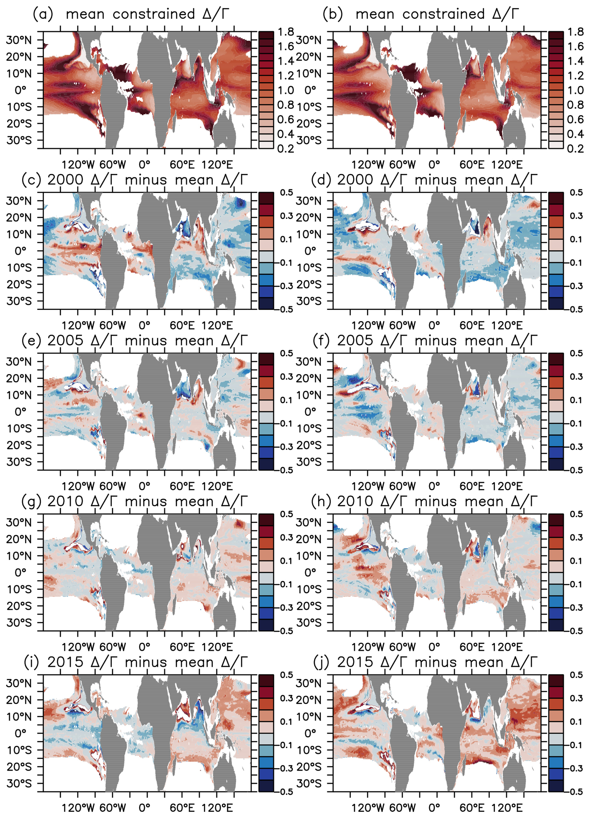
Figure 5 The Δ $/$ Γ constrained by the simulated concentration of CFC-12 and SF₆ on isopycnal layer σ₀=25.5 kg m⁻³ under preindustrial and historical forcing conditions. Panels (c), (e), (g), and (i) show Δ $/$ Γ constrained in 2000, 2005, 2010, and 2015 minus the temporal mean Δ $/$ Γ (a) in the esm-piControl experiment. Panels (d), (f), (h), and (j) show Δ $/$ Γ constrained in 2000, 2005, 2010, and 2015 minus the temporal mean Δ $/$ Γ (b) in the esm-hist experiment. During the calculation, we assumed 100 % surface saturation of both tracers.

The Δ $/$ Γ ratio constrained by both CFC-12 and SF₆ in the esm-piControl simulations shows substantial spatial differences but, somehow, temporal consistency (Fig. 5a, c, e, g, i). Small Δ $/$ Γ ratios, i.e., corresponding to weak water mass mixing, are diagnosed mainly in the subtropical gyres of the Southern Hemisphere, whereas high Δ $/$ Γ ratios are diagnosed in the tropical areas where different water masses mix along the isopycnal. The temporal consistency of the constrained Δ $/$ Γ ratios reflects the validity of the essential steady-state assumption of the TTD method under preindustrial conditions. It allows for the application of Δ $/$ Γ constrained by the CFC-12–SF₆ pair over the past in the IG-TTD calculation. For instance, given that SF₆ measurements are primarily available post-2000, whereas CFC-12 measurements have been extensively recorded since 1980, we can use the CFC-12–SF₆ pair to constrain the Δ $/$ Γ ratio in 2000 or later. Subsequently, we can employ this ratio, along with CFC-12 measurements before 2000, to calculate the IG-TTD. However, under a transient climate state with internal variation and underlying trends, the Δ $/$ Γ ratios show slightly more temporal changes (Fig. 5b, d, f, h, j).

Applying a constrained Δ $/$ Γ ratio to the full time series in the esm-piControl simulation still leads to systematic underestimates of the simulated ideal age by IG-TTD, but it helps to find robust temporal trends and variability in the water age (Fig. 6b, Table S1 in the Supplement). Results show that globally averaged Γ underestimates the simulated ideal age by around 43 %, which is similar to the performance of IG-TTD when using Δ $/$ Γ=1. In terms of temporal variability, the correlation coefficient of the globally averaged Γ and ideal age is above 0.9. Moreover, the temporal trend in Γ overlaps with the trend in ideal age at the 95 % confidence interval (Table S1).

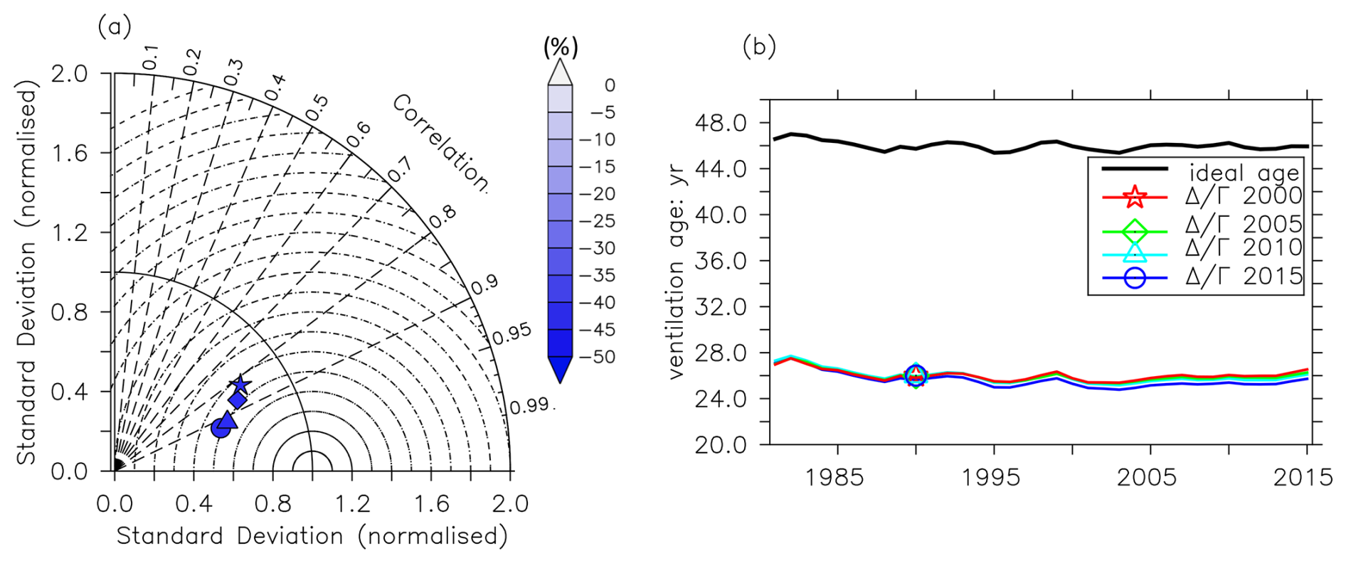
Figure 6 The same as Fig. 3 but with a different assumption regarding the IG-TTD calculation. Here, we use the Δ $/$ Γ constrained by CFC-12 and SF₆ in different years. Symbols reveal the year in which the Δ $/$ Γ is constrained: a star indicates 2000, a diamond indicates 2005, a triangle indicates 2010, and a circle indicates 2015. Panel (b) shows time series of the globally averaged ideal age (black) and mean age of IG-TTD with Δ $/$ Γ constrained in 2000 (red), 2005 (green), 2010 (cyan), and 2015 (blue).

4.4 IG-TTD with time-varying surface saturation of tracers in the esm-piControl simulations

As Eq. (3) suggests, the IG-TTD at location r is solved with the ocean interior tracer concentration c(r,t) and its surface history c₀(t,ξ), where the latter is determined not only from the atmospheric tracer history but also from the tracer saturation state. The latter is usually assumed to be 100 % (e.g., Waugh et al., 2004); however, this assumption is not realistic everywhere, especially in high-latitude regions. Both observations and model simulations have shown considerable undersaturation in deep-convection regions due to the entrainment of older, subsurface water masses that typically have lower concentrations of anthropogenic transient tracers (Tanhua et al., 2008; Shao et al., 2013; He et al., 2018; Raimondi et al., 2021). Moreover, the saturation state also evolves with time due to changes in factors such as the atmospheric partial pressure of transient tracers, the re-entrainment of young waters, the oceanic mixed-layer depth, and ocean warming. The assumption of tracer saturation constitutes a considerable uncertainty in IG-TTD applications in such regions (Shao et al., 2013; Stöven et al., 2015).

In order to explicitly account for the time-varying saturation of CFC-12 and SF₆ in the TTD calculation, we adjusted the mixing ratio histories of CFC-12 and SF₆. These adjustments were made based on the simulated saturation of CFC-12 and SF₆ at outcrops under hemispheric winter conditions, i.e., March in the Northern Hemisphere and September in the Southern Hemisphere, given that water mass formation (ventilation) takes place in early spring. Here, the term “outcrop” refers to the place in which an isopycnal (or potential density layer) emerges at the surface and exchange with the atmosphere occurs. The CFC-12 and SF₆ surface saturation values calculated for σ₀=25.45 kg m⁻³ to 25.55 kg m⁻³ along the outcrops in the Atlantic Ocean, Pacific Ocean, Indian Ocean, Arctic Ocean, and Southern Ocean range from 80 % to 100 % (Fig. S3). Finally, IG-TTD applying adjusted mixing ratio histories of CFC-12 and SF₆ are calculated and compared with the ideal age (see details in Text S1 in the Supplement).

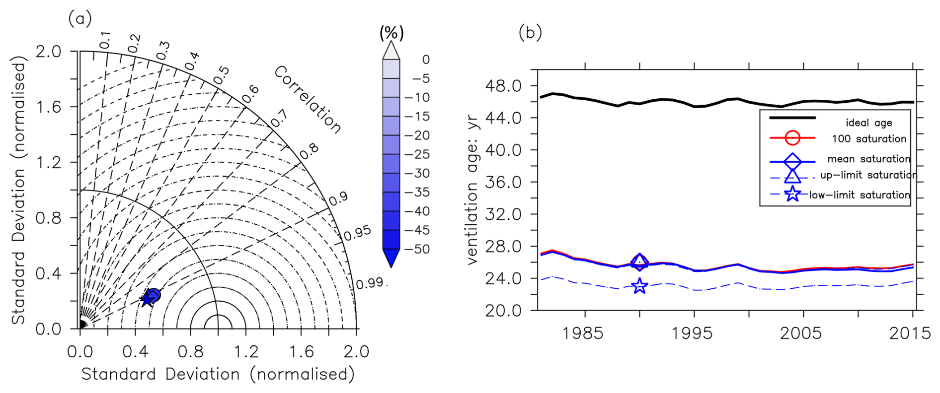
Figure 7 The same as Fig. 3 but with a different assumption regarding the IG-TTD calculation. Here, we use the Δ $/$ Γ constrained by CFC-12 and SF₆ in 2015, considering 100 % surface saturation (circle) and the time-varying surface saturation of CFC-12 and SF₆ (mean saturation state: triangle; upper-limit saturation state: diamond; lower-limit saturation state: star) in all ocean basins. Panel (b) shows time series of the globally averaged ideal age (black), the mean age under a 100 % saturation assumption (red), and the solid values of the mean age of IG-TTD considering the mean temporal change in the CFC-12 saturation over outcrops (solid blue) and the change in the upper-limit (upper blue dash) and lower-limit CFC-12 (lower blue dash) saturation state.

Considering temporally varying saturation of CFC-12, the Γ value is systematically younger than that assuming 100 % saturation (Fig. 7), as suggested by other studies (Shao et al., 2013; He et al., 2018). The Γ value calculated with a 100 % saturation assumption is 0.14 years (with the upper limit of actual surface saturation) and 2.49 years (with the lower limit of actual surface saturation) older than the Γ value considering temporally varying saturation. The difference between a 100 % saturation mean age and a temporally varying saturation mean age is supposed to be larger in the deeper ocean because of the more pronounced undersaturation state in the higher-latitude regions (He et al., 2018). Notably, the assumption of 100 % saturation is, however, a minor contributor to the bias of the mean age from IG-TTD compared with the ideal age in the upper tropical thermocline. This finding aligns with other independent model studies conducted by Shao et al. (2016) and He et al. (2018).

Moreover, the assumption of 100 % surface saturation has minimal impact on the spatial pattern, temporal variability, or trends in horizontally averaged Γ in the upper thermocline σ₀=25.5 kg m⁻³ (Fig. 7). The spatial correlation coefficients between Γ and the ideal age are all around 0.9 under various surface saturation assumptions. The Pearson correlation coefficients between the mean age of IG-TTD assuming 100 % surface saturation, upper-limit surface saturation, mean surface saturation, lower-limit surface saturation, and ideal age are all above 0.8. Except for Γ considering the mean surface saturation of both tracers, the trends in Γ are the same as the temporal trend in ideal age at the 95 % confidence interval. Considering the mean surface saturation state of CFC-12 and SF₆, Γ changes at a rate of $-\mathrm{0.050}\pm \mathrm{0.013}$ yr yr⁻¹, which is slightly different from the trend in the ideal age ($-\mathrm{0.016}\pm \mathrm{0.012}$ yr yr⁻¹).

4.5 IG-TTD trends in esm-hist simulations

One application of the mean age of TTD derived from CFCs and SF₆ is to monitor potential changes in ventilation under transient climate conditions, which can be caused, for example, by changes in wind or upper-ocean stratification, as shown in Waugh et al. (2013) for the Southern Ocean and in Jeansson et al. (2023) for the Nordic Seas. Here, we present the trends in the ideal age and TTD-based mean age in our esm-hist simulation, where anthropogenic forcings have been incorporated in the fully coupled FOCI ESM. We assume either spatially homogeneous Δ $/$ Γ ratios (0.8, 1.0, 1.2, and 1.4) or CFC-12- and SF₆-constrained Δ $/$ Γ ratios as well as a 100 % surface saturation assumption for both tracers to calculate the IG-TTD.

Under the assumption of a spatially homogeneous Δ $/$ Γ (0.8, 1.0, 1.2, and 1.4), our results suggest that Γ constrained by CFC-12 alone is not able to detect the ideal age change in the esm-hist simulation (Fig. 8a, Table S2). The ideal age and the AOU increase at respective rates of 0.056±0.019 yr yr⁻¹ and 0.122±0.013 mmol m⁻³ yr⁻¹ (not shown) during the period from 1981 to 2015, indicating an overall weakening ventilation at the upper isopycnal layer σ₀=25.5 kg m⁻³. The single-tracer-constrained Γ effectively captures the slowdown in ventilation during the years 1990 and 2006 (the small spikes in the ideal age and in all mean ages in Fig. 8a). However, globally averaged Γ assuming spatially homogeneous Δ $/$ Γ changes at rates of 0.115±0.020 yr yr⁻¹ (Δ $/$ Γ=0.8), $-\mathrm{0.009}\pm \mathrm{0.020}$ yr yr⁻¹ (Δ $/$ Γ=1.0), $-\mathrm{0.151}\pm \mathrm{0.022}$ yr yr⁻¹ (Δ $/$ Γ=1.2), and $-\mathrm{0.313}\pm \mathrm{0.026}$ yr yr⁻¹ (Δ $/$ Γ=1.4); i.e., temporal trends in Γ significantly differ from that of the ideal age in the esm-hist simulation (Table S2). Our earlier finding of strong trends in Γ under stable climate conditions (the esm-piControl experiment; Fig. 3b, Table S1), where no trend is expected, supports the conclusion that the respective single-tracer Γ trends in esm-hist are artificial and unreliable.

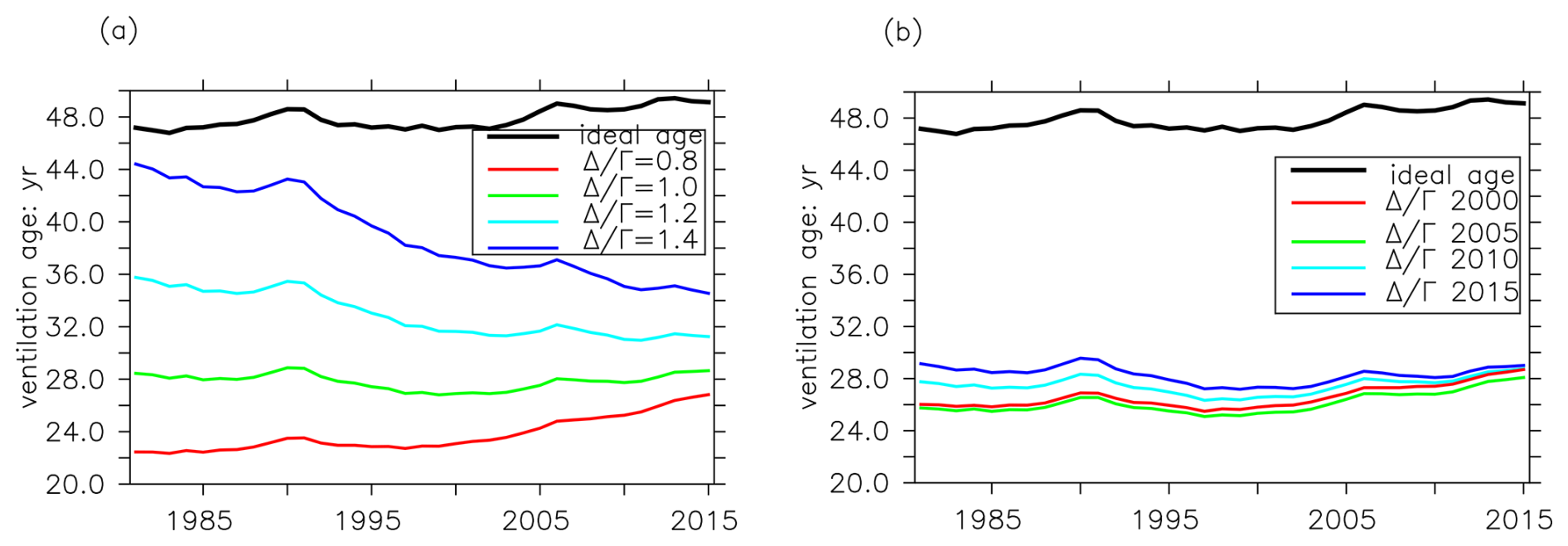
Figure 8 Trends in the globally averaged ideal age and Γ for various Δ $/$ Γ assumptions for the esm-hist experiment at the density layer σ₀=25.5 kg m⁻³. (a) Globally averaged ideal age (black) and mean age from CFC-12-based IG-TTD using spatially homogenous Δ $/$ Γ values (red: 0.8; green: 1.0; cyan: 1.2; and blue: 1.4) from 1981 to 2015 in the historical simulation. (b) The globally averaged ideal age (black) and mean age of IG-TTD using CFC-12- and SF₆-constrained Δ $/$ Γ values. In panel (b), the line color represents the year in which the Δ $/$ Γ ratio has been constrained (red: 2000; green: 2005; cyan: 2010; blue: 2015). A value of 100 % surface saturation of both CFC-12 and SF₆ is assumed for all calculations.

Using Δ $/$ Γ constrained by the CFC-12–SF₆ tracer pair in the esm-hist simulations, the difference between the temporal trends in the globally averaged Γ and the ideal age becomes significantly narrower (Fig. 8b, Table S2). Using Δ $/$ Γ constrained in 2000 and 2005, the temporal trends in Γ are 0.064 ± 0.019 and 0.055±0.020 yr yr⁻¹, respectively, which is in line with the temporal trend in the ideal age at the 95 % confidence interval. Furthermore, the Pearson correlation coefficients between the respective globally averaged Γ and the ideal age are 0.947 and 0.949. In other words, the mean age from constrained IG-TTD is able to detect the temporal variability and trend in the simulated ideal age. In contrast, when using Δ $/$ Γ constrained in 2010 and 2015, globally averaged Γ values indicate no significant trend (0.017±0.021 and $-\mathrm{0.016}\pm \mathrm{0.021}$ yr yr⁻¹, respectively) but still show better performance than when using a spatially homogeneous Δ $/$ Γ ratio.

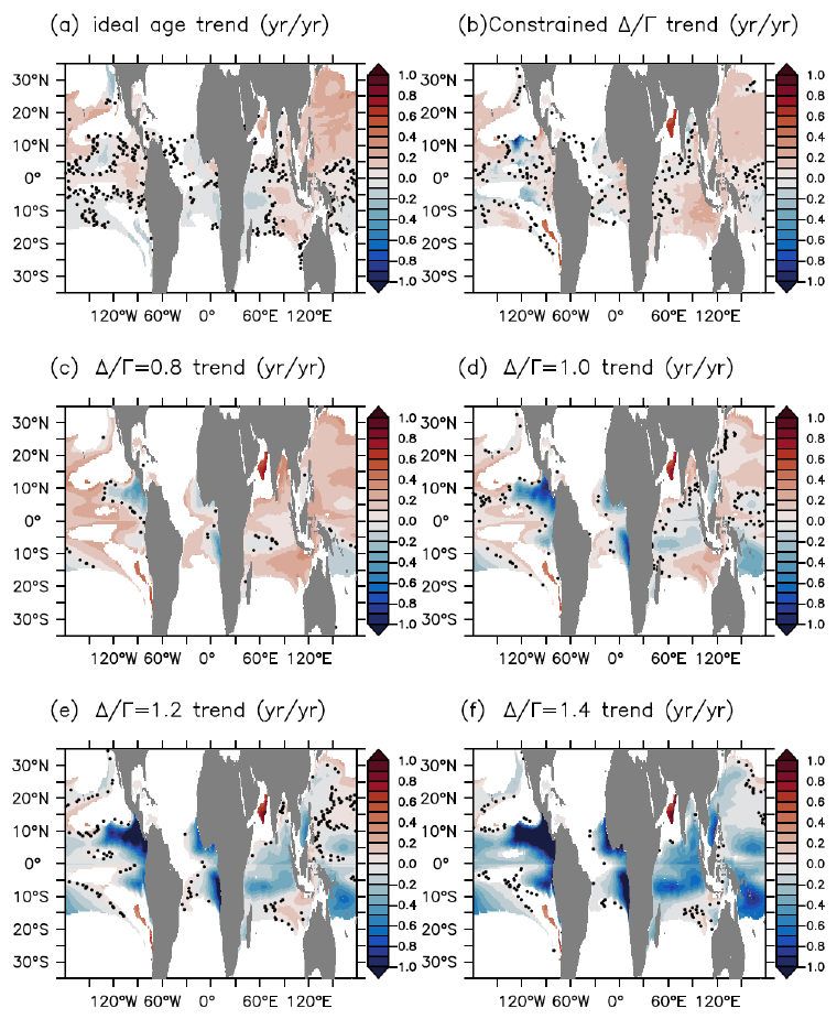
Figure 9 Temporal trends in the ideal age (a, in unit of yr yr⁻¹) and the mean age of IG-TTD with different assumptions with respect to the value of Δ $/$ Γ (b–f, in unit of yr yr⁻¹) on isopycnal layer σ₀=25.5 kg m⁻³ in the esm-hist simulation. Stippling designates areas in which the ratio of the standard deviation and mean of the regression slope of the ideal age (or mean age) against time exceeds 1 (i.e., no significant trends).

It is noteworthy that the dual-tracer-constrained IG-TTD demonstrates superior performance with respect to discerning the spatial patterns and magnitude of temporal changes in the ideal age compared to the single-tracer-constrained IG-TTD (Fig. 9). The single-tracer-constrained IG-TTD is very sensitive to the chosen value of Δ $/$ Γ, commonly showing a spurious age increase with low values of Δ $/$ Γ and an age decrease with high values of Δ $/$ Γ across all ocean basins (Fig. 9c–f). While the dual-tracer method exhibits some spurious trends in the eastern tropical Atlantic and western tropical Indian Ocean, it generally provides a more accurate representation of the spatial patterns and magnitudes of true ideal age trends. Notably, it correctly identifies regions with no significant trends in the ideal age (Fig. 9a, b).

5 Discussion

Over the last 4 decades, extensive measurements of dissolved anthropogenic gases, such as CFCs and SF₆, have been conducted in the global ocean (Lauvset et al., 2022) through programs like the World Ocean Circulation Experiment (WOCE) and the Global Ocean Ship-Based Hydrographic Investigation Program (GO-SHIP). These measurements provide valuable data for diagnosing the spatial patterns and temporal changes in seawater age, anthropogenic carbon storage, and biogeochemical processes, such as respiration, using the IG-TTD technique. A recent study by Jeansson et al. (2023) shows overall stronger ventilation in the Greenland Sea from the 1990s to the 2010s, in line with the results revealed by the AOU. As for biogeochemical processes, many field studies use the mean age of IG-TTD as the seawater age (Álvarez-Salgado et al., 2014; Sonnerup et al., 2013, 2015; Sulpis et al., 2023) to diagnose regionally averaged oceanic aerobic respiration rates by calculating the OUR (i.e., the slope of the least-squares regression of the AOU and seawater age on potential density surfaces) (Jenkins, 1987; Guo et al., 2023).

Nevertheless, uncertainties associated with the IG-TTD technique, including its ability to accurately represent the climatological mean, spatial variance, and temporal trends in the “true” seawater age, may hinder its direct applicability. Our study suggests that, across all tested assumptions, the mean age derived from the IG-TTD method tends to underestimate the ideal age within the upper thermocline. Such underestimation is also the case for the simple CFC-12 and CFC-11 mixing ratio age (Thiele and Sarmiento, 1990; Mecking et al., 2004). This discrepancy could potentially affect the estimation of ocean heat uptake and anthropogenic carbon storage when relying on IG-TTD mean ages in certain oceanic regions. Additionally, uncertainties in the spatial variance of the mean age of IG-TTD might further limit the application for OUR computation, as the OUR is calculated from spatial gradients of Γ and the AOU in the real ocean. The third caveat of the IG-TTD technique is that the temporal trend in the mean age might not faithfully reflect the temporal changes in the ocean ventilation unless the Δ $/$ Γ ratio can be constrained by dual transient tracers (whenever available). We have shown that applying an additional tracer (SF₆) with a different input function in the IG-TTD technique improves the estimate of temporal changes in the ocean ventilation strength. Moreover, in the Nordic Seas, where SF₆ has been deliberately released in the past, potential future measurements of Argon-39 combined with CFC-12 measurements may be used to locally constrain the Δ $/$ Γ ratio (Ebser et al., 2018).

Why does the mean age of IG-TTD tend to underestimate the ideal age? Firstly, the IG-TTD technique assumes a spectrum of transit timescales of water parcels following a unimodal IG distribution. However, this might not be an accurate assumption in oceanic regions with complex circulation. Studies by Haine and Hall (2002), Peacock and Maltrud (2006), Shao et al. (2016), and Chouksey et al. (2022) suggest that TTD distributions often exhibit a bimodal or multimodal structure in upwelling and downwelling regions as well as in regions where multiple source water masses converge (such as the equatorial region and the Southern Ocean). For example, Peacock and Maltrud (2006) compared the concentration of a CFC-like tracer via the convolution of the ocean surface CFC boundary condition with the model-simulated TTD (“actual” CFC) and the one derived from the same boundary condition with the IG-TTD (“predicted” CFC). Both TTD and IG-TTD share the same Γ and Δ. They found that the predicted CFC-like concentrations are only half of the actual values at a depth of 245 m in the tropical regions (see their Fig. 13). In other words, to achieve the same abiotic transient tracer concentration inferred from model-simulated TTD, the IG-TTD mean age would need to be reduced; i.e., the mean age of IG-TTD is smaller than the mean age of the real TTD with the same CFC partial pressure. To narrow down the discrepancy between the ideal age and mean age of TTD, linear combinations of IG distributions can be used (Eq. 7), as proposed by Waugh et al. (2003) and Steinfeldt et al. (2024). However, incorporating additional source water masses in the analysis requires additional transient tracers with different atmospheric histories to constrain the Δ $/$ Γ ratios, as well as the respective water fractions characterizing the multimodal IG distribution, as mentioned by Stöven et al. (2016). With a limited number of transient tracers available from observations and in our model experiments, the multimodal TTD cannot be solved in this study.

Another potential reason for the disparity between the ideal age and mean age of IG-TTD is the limited atmospheric history length of CFC-12 and SF₆ (Shao et al., 2016). These gases were released into the atmosphere after 1936 and 1953, respectively, currently providing a historical span of only 88 years for CFC-12 and 71 years for SF₆ (Bullister, 2015). Therefore, the extended tail of older ages in the spectrum cannot be adequately constrained by these tracers alone. Incorporating additional age tracers with longer atmospheric histories or lifetimes, such as Argon-39 with a half-life of 269 years, might offer better constraints on older water components in the transient age spectrum and help reduce the disparity between the IG-TTD and ideal age. To provide more details, a set of simulations of CFC-12, SF₆, Argon-39, and ideal age is required.

$$\begin{array}{}\text{(7)}& \begin{array}{rl}G(\mathit{r},\mathit{\xi })& ={\mathit{\alpha }}_{\mathrm{1}}{G}_{\mathrm{1}}({\mathrm{\Gamma }}_{\mathrm{1}},{\mathrm{\Delta }}_{\mathrm{1}})+{\mathit{\alpha }}_{\mathrm{2}}{G}_{\mathrm{2}}({\mathrm{\Gamma }}_{\mathrm{2}},{\mathrm{\Delta }}_{\mathrm{2}})+\mathrm{\dots }\\ & +{\mathit{\alpha }}_n{G}_n({\mathrm{\Gamma }}_n,{\mathrm{\Delta }}_n)\end{array}\end{array}$$

Continuous measurements of CFC-12, SF₆, and (hopefully) additional transient tracers (e.g., ³⁹Ar) with a different and longer atmospheric history, along with techniques for separating source water masses, might help to better quantify ocean ventilation. Our study confirms the better performance of IG-TTD when dual transient tracers (CFC-12 and SF₆) are utilized, compared to the case of using only a single tracer (CFC-12), and that measurements of transient tracers that have longer atmospheric histories might further improve the performance of TTD with respect to representing old waters (Shao et al., 2016). Water fractions, required in Eq. (7), can be derived by applying the optimal multiparameter (OMP) analysis (Karstensen and Tomczak, 1998).

6 Conclusion

Our study evaluates the inverse Gaussian transit time distribution (IG-TTD) method by comparing the mean age of IG-TTD (Γ) and a ground truth measure of water age, the ideal age on the isopycnal layer σ₀=25.5 kg m⁻³ within an Earth system model. Our results suggest the following:

• i.

  Γ substantially underestimates the ideal age of 46.0 years by up to 24.3 years. Such a difference might arise from the assumption that the transit time distribution of water parcels follows the unimodal inverse Gaussian distribution and from the limited atmospheric history length of CFC-12 and SF₆, which cannot well constrain the long tail towards high ages in the spectrum.

• ii.

  Possibly incorrect assumptions about surface saturation of CFC-12 and SF₆ do not resolve the discrepancy between Γ and the ideal age.

• iii.

  When only CFC-12 is used (assuming spatially homogeneous Δ $/$ Γ of 0.8, 1.0, 1.2, and 1.4), the derived Γ shows significantly different trends from 1981 to 2015 compared to the ideal age, indicating a misrepresentation of temporal change in the ocean ventilation inferred by the IG-TTD technique in this case.

• iv.

  When dual tracers (CFC-12 and SF₆) are used in the IG-TTD techniques, Γ can correctly detect temporal variability and trend in the true water age in the upper tropical thermocline.