A global summary of seafloor topography influenced by internal-wave-induced turbulent water mixing

Turbulent water motions are important for the exchange of momentum, heat, nutrients, and suspended matter, including sediments in the deep sea. The motions occur in a deep sea that is generally stably stratified in density. To maintain ocean–density stratification, an irreversible diapycnal turbulent transport is needed. The geological shape and texture of marine topography are important for water mixing, as most deep-sea turbulence is generated via internal waves breaking at sloping seafloors. For example, slopes of semidiurnal internal tidal characteristics can “critically” match the mean seafloor slope. In this paper, the concept of critical slopes is revisited from a global internal-wave turbulence viewpoint using seafloor topography and moored high-resolution temperature sensor data. Observations suggest that turbulence generation via internal-wave breaking at 5 % ± 1.5 % of all seafloors is sufficient to maintain ocean–density stratification. However, most, >90 %, turbulence contributions are found at supercritical, rather than the more limited critical, slopes measured at 1^′ scales that cover about 50 % of seafloors at water depths <2000 m. Internal tides (∼60 %) dominate over near-inertial waves (∼40 %), which is confirmed by comparison of northeastern Atlantic data and eastern Mediterranean data (weak tides) at the same mid-latitude. Seafloor elevation spectra show a wavenumber (k) falloff rate of k⁻³, which is steeper than what was found previously. The falloff rate is even steeper, resulting in less elevation variance in a 1-order-of-magnitude bandwidth around k_T=0.5 cycle km⁻¹. The corresponding length is equivalent to the internal wave excursion length. The reduction in seafloor elevation variance seems to be associated with seafloor erosion by internal wave breaking. The potential robustness of the seafloor and internal wave interaction is discussed.

1 Introduction

The present ocean has existed for millions of years, and so seemingly have its seafloor shape and water flows, including properties like the stable vertical stratification in density from heating by the Sun. Because sedimentation and erosion of suspended matter in the ocean are subject to water flows that partially depend on interaction with the seafloor, one may question the stability or variability of seafloor shape and water flow properties. Compared with geological timescales of variation (sedimentary: years; rocks: centuries or millennia), water flows in the deep ocean are fast-fluctuating (mesoscale eddies: weeks or months; tides: hours or days). However, this does not preclude potential interactions between water flows and topographic bedforms with local results such as sand ripples and sediment waves (e.g., Trincardi and Normark, 1988; Puig et al., 2007).

As seafloor erosion by resuspension is mainly driven by intense water turbulence and seafloor deposition by weak turbulence, seafloor shaping such as contourite morphology (e.g., Rebesco et al., 2014; Chen et al., 2022) depends on dominant ocean turbulence generation processes. Following, e.g., Wunsch (1970), Eriksen (1982), Thorpe (1987), Klymak and Moum (2003), Hosegood et al. (2004), and Sarkar and Scotti (2017), ocean turbulence above sloping seafloors is predominantly generated by the breaking of internal water waves. The turbulence produced by the breaking of internal waves is considered vital for the global ocean meridional overturning circulation (e.g., St. Laurent et al., 2012). Such waves are mainly supported by the stable vertical density stratification. Their effects on shaping the ocean's seafloor morphology cannot be overstated (Rebesco et al., 2014).

More generally, balanced feedback interaction leading to a quasi-stable equilibrium is expected between the slopes of seafloor topography and long-lasting ubiquitous water flows, e.g., generated by internal waves that are notably driven by oscillating tides and the waves' density stratification support. In their pioneering works, Bell (1975a, b) from an internal wave generation perspective, Cacchione and Wunsch (1974) and Eriksen (1982, 1985) from an internal wave breaking perspective, and Cacchione and Southard (1974) from a geological formation perspective suggested that a “critical” match exists between the mean angles of deep-sea topography slopes and those of internal wave “characteristics”.

Because internal water waves are essentially three-dimensional (3D) phenomena, which distinguishes them from 2D surface waves, their energy propagates along characteristics, i.e., paths that slope to the horizontal as a function of wave frequency, latitude, and stratification. Internal waves can reflect off a seafloor slope, but due to angle preservation with respect to gravity instead of bottom normal, internal wave energy is thought to build up when two slopes are identical, yielding potential propagation parallel to a critical seafloor slope (Cacchione and Wunsch, 1974). When the seafloor slope is larger than the internal wave slope, it is supercritical, and when it is smaller than the internal wave slope, it is subcritical (for that particular wave frequency under given stratification conditions).

While Bell (1975a, b) considered seafloor elevation statistics on internal wave generation, the works of Cacchione and co-authors considered seafloor shaping by internal wave motions. It was found that the average seafloor slope amounts to 3 ± 1°, which matches the characteristic slope of the energy propagation direction of internal waves at a semidiurnal tidal frequency for stratification from around 1700 m below the sea surface, which is about half the average water depth.

While the above finding is remarkable and has led to numerous investigations into critical reflection of internal waves, it is challenged by various perspectives. This is because, first, exactly matching “critical” slopes for dominant internal tides are few and far between and cannot persist in space and time as the ocean stratification varies in space and time. Second, internal waves mostly break above sloping topography and very little in the ocean interior (Polzin et al., 1997). Third, most ocean seafloors, i.e., 75 % by area and 90 % by volume (Costello et al., 2010, 2015), are located between 3000 and 6000 m water depths, where density stratification is relatively weak. Fourth, about 40 % of the total internal wave energy is estimated at near-inertial frequencies (e.g., Wunsch and Ferrari, 2004).

Near-inertial waves are generated as transients following geostrophic adjustment of the rotating Earth, e.g., after passing atmospheric disturbances or frontal collapses (LeBlond and Mysak, 1978). Their occurrence shows strong variability with location, e.g., demonstrating large near-surface generation in western boundary flows and much weaker generation in eastern ocean basins (Watanabe and Hibiya, 2002; Alford, 2003). As near-inertial waves have a quasi-horizontal component, virtually all of the seafloor slopes are steeper: they are supercritical (for near-inertial waves). These observations demand further investigation of the seafloor–internal wave turbulence interaction, also considering the potential impact on climate variability and the contribution of oceans to distributing heat therein.

Detailed ocean observations indicate that most of the intense turbulence and sediment resuspension over sloping seafloors is not generated by frictional (shear) flows (as suggested by, e.g., Cacchione et al., 2002) but by nonlinearly deformed internal wave breaking (e.g., Klymak and Moum, 2003; Hosegood et al., 2004). Such nonlinear internal wave breaking predominantly generates buoyancy-driven convection turbulence. Growing evidence suggests that most breaking occurs at slopes that are just supercritical (e.g., van Haren et al., 2015; Winters, 2015; Sarkar and Scotti, 2017).

Any interaction between seafloor shape and texture and water flow turbulence is expected to vary on geological timescales, because, besides deep-sea topography, ocean-internal vertical density stratification has existed as long as oceans have. The ocean is not and has not been a pool of stagnant cold water underneath a thin layer of circulating warm water heated by the Sun (Munk and Wunsch, 1998). The question is how stable the balance of such an interaction can be, e.g., between internal waves that are supported by varying stratification and seafloor topography. Is the balance an optimum or rather a marginal equilibrium, like the marginally stable stratification supporting maximum destabilizing internal shear in shelf seas (van Haren et al., 1999)? Especially given relatively rapid changes, such as Earth surface heating attributed to humans, does a balance buffer any modifications to topography (long timescale), vertical density stratification (medium timescale), and/or water flow (short timescale)? Prior to being able to (mathematically) predict any potential tipping point of a balance, the physical processes that contribute to a balance need to be understood. Amongst other deep-sea processes, this involves understanding the physics of internal wave formation and breaking into turbulence generation upon interaction with topography and re-stratification of density.

In this paper, we discuss the (im)possibility of relating seafloor statistics to open-ocean density stratification and internal wave breaking as observed in recent measurements. We revisit the concepts of deformation, erosion, and sedimentation as well as deep seafloor topography in interaction with internal waves, vertical density stratification, turbulence, and ocean heating or cooling, and we consider the (in)stability of these interactions. Instead of the Bell (1975a, b) perspective of internal wave generation, above the northeastern Pacific abyssal hills, we adopt the perspective of internal wave breaking and turbulence generation through moored high-resolution temperature “T”-sensor observations from mean results above a wide variety of deep-ocean topographies and detailed results of two representative mid-latitude sites (φ=37° N) (Fig. 1). We also adopt a geological seafloor topography perspective using some detailed multibeam echo sounder and global seafloor elevation repository data. An attempt is made to consider the statistical spread of the different variables.

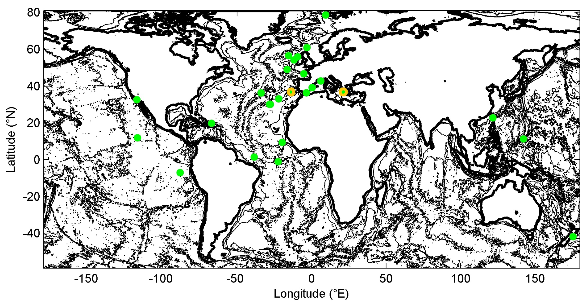
Figure 1 Global map of seafloor topography (1^′ version of Smith and Sandwell, 1997) with contours every 1500 m, together with sites (green dots) of NIOZ T-sensor moorings for deep-sea turbulence and internal wave research, of which contributions to the mean values are used in this study. The two orange encircled sites are discussed in some detail.

2 Internal wave–topography interactions

2.1 Some considerations on ocean variability and internal wave–topography interactions

Large variability of over 2 orders of magnitude exists in stable ocean–density stratification (∼N²), though a gradual not constant decrease with increasing depth is observed in buoyancy frequency N, which is a measure of stability of a stratified fluid to vertical displacements (e.g., Wüst, 1935; Wunsch, 2015). This gradual decrease with depth results in a corresponding increase in the slope β to the horizontal along which internal wave energy characteristics propagate. For general ocean stratification, this slope is approximately inversely proportional to N (e.g., LeBlond and Mysak, 1978),

$$\begin{array}{}\text{(1)}& \mathit{\beta }={\sin }^{-\mathrm{1}}\left(\right({\mathit{\omega }}^{\mathrm{2}}-f^{\mathrm{2}}{)}^{\mathrm{1}/\mathrm{2}}/(N^{\mathrm{2}}-f^{\mathrm{2}}{)}^{\mathrm{1}/\mathrm{2}}),\end{array}$$

for freely propagating linear internal waves at frequency ω. Here, f denotes the inertial frequency or Coriolis parameter, which is the vertical component of planetary vorticity. Internal waves and subinertial water flows deform the stratification locally, thereby making N a function of time and space $N=N(x,y,z,t)$. The consequences of variability for β will be explored from the observations in Sect. 4.

Several global internal wave statistics can be given. The rms-mean deep-sea topography slopes of 3 ± 1° (Bell, 1975b; Cacchione et al., 2002) roughly match the mean slope of (linear) semidiurnal internal tide characteristics, provided the latter are computed using in Eq. (1) a value of $N\approx \mathrm{2}\times {\mathrm{10}}^{-\mathrm{3}}$ s⁻¹ for mid-latitude locations. Such an N is found around approximately $z=-\mathrm{1700}$ m in the open ocean, which has a mean seafloor depth of H=3900 m outside shelf seas (Wunsch, 2015). In these open-ocean mid-depth waters, internal wave breaking and thus turbulence generation are sparse (e.g., Gregg, 1989; Polzin et al., 1997; Kunze, 2017).

Observational evidence suggests that vigorous turbulent mixing by internal wave breaking is only found at a limited height of h=100–200 m (e.g., Polzin et al., 1997) above the seafloor, coarsely estimated to occur over only 5 %–15 % of all seafloor slopes to maintain the ocean stratification (e.g., van Haren et al., 2015). As for the relevant length scales, although satellite altimetry observations demonstrate low-mode internal tides with wavelengths O(100) km (e.g., Dushaw, 2002; Ray and Zaron, 2016), the excursion length of internal tides is typically O(1) km, which may prove important for turbulence generation and thus sediment erosion of seafloor texture and topography.

The smaller length scale O(1) km especially may fit the spectral analysis of northeastern Pacific seafloor elevation, which is found to fall off with a horizontal wavenumber (k) like k^−2.5 (Bell, 1975a); this was later corrected to k⁻² (Bell, 1975b). The latter is interpreted as a random distribution of hills in which the energy of the formation is distributed uniformly over all sizes. Internal wave generation was found by Bell (1975a, b), mainly in the interval $\mathrm{0.33}<k<\mathrm{3}$ cpkm (short for cycles per kilometer). Here, we add that this roughly matches a band with an increased spread of topographic height variance in the interval $\mathrm{0.15}<k<\mathrm{1}$ cpkm, which is visible in the presented data but not mentioned by Bell (1975a, b).

Geomorphology influences water flow and turbulence, and these in turn influence sediment erosion and deposition and thus (fine-tuning) geomorphology. So, if enough time is available (after all, geologists think in terms of millions of years), one will eventually reach an equilibrium. The major geomorphological processes occur on a much longer timescale than the adaptation of water flows, and any ocean will “always” be in an equilibrium situation because the flows adapt relatively quickly to a slow geological change.

Thus, following variations in ocean internal wave turbulence, the seafloor topography will adapt. However, the ocean also interacts with a faster adaptive or varying system: the atmosphere. Temperature changes in water are slower than in air because of the larger heat capacity of the former. Nevertheless, a direct correspondence to changes in vertical density (temperature) stratification is not evident, as greater stratification can support more internal waves and thus potentially more turbulent wave breaking that may restore a balance.

The dominant sources of ocean internal waves are tides (e.g., Wunsch and Ferrari, 2004). The local seafloor slope γ, computed over a certain horizontal distance, is supercritical for linear freely propagating semidiurnal lunar internal tidal waves at ω=M₂, when γ>β_M2 using ${\mathit{\omega }}_{M\mathrm{2}}=\mathrm{1.405}\times {\mathrm{10}}^{-\mathrm{4}}$ s⁻¹ in Eq. (1).

A secondary source is near-inertial waves at ω≈f, which generally have a near-horizontal slope of characteristics. Only with very weak stratification N=O(f) may some near-inertial slopes become large enough to distinguish between various subcritical slopes for such waves. However, under weakly stratified conditions, terms involving the horizontal Coriolis parameter are no longer negligible, and two distinctly differently sloping characteristics μ_± of internal wave energy propagation result (e.g., LeBlond and Mysak, 1978; Gerkema et al., 2008):

$$\begin{array}{}\text{(2)}& {\mathit{\mu }}_{\pm }=(B\pm (B^{\mathrm{2}}-AC{)}^{\mathrm{1}/\mathrm{2}})/A,\end{array}$$

where $A=N^{\mathrm{2}}-{\mathit{\omega }}^{\mathrm{2}}+f_s^{\mathrm{2}}$, B=ff_s, $C=f^{\mathrm{2}}-{\mathit{\omega }}^{\mathrm{2}}$, and f_s=f_hsin α. α is the angle to φ. The slopes of μ_± indicate directions to the horizontal in a more general way than the single slope (Eq. 1) obtained using the traditional approximation. The variation of Eqs. (1) and (2) as a function of N will be compared with statistics of seafloor slopes computed at various length scales in Sect. 4.

For large N≫f, the slopes of the two characteristics in Eq. (2) approach each other, and their slopes approach β in Eq. (1). Under conditions N<10f and latitudinal propagation ($\mathit{\alpha }=\mathit{\pi }/\mathrm{2}$), one of the characteristics in Eq. (2) becomes quasi-horizontal, for which virtually all seafloor slopes are supercritical, and the other becomes more steeply sloping.

The impact of Eq. (2) may also not be ignorable for semidiurnal tides in weakly stratified waters around mid-latitudes. With the full non-approximated Eq. (2) and a stratification of about N=8f, which is typical in waters near the 3900 m mean depth of the ocean seafloor, the slope Eq. (1) of β_M2=9.1° rather becomes 10.3 and 7.9° for up-going and down-going characteristics μ_± (for $\left|\mathit{\phi }\right|=\mathrm{37}\mathit{°}$).

This spread of about ±13 % is a substantial addition to variation in seafloor slope criticality and becomes larger at weaker stratification (N<8f) and smaller at stronger stratification (N>8f). Although the vertical density stratification is generally a monotonic decreasing function with increasing depth, deviations occur, such as in some, e.g., equatorial areas around 4000 m, where a larger N is found than above and below and which is attributed to the transition between deep Arctic waters overlying most dense Antarctic waters (King et al., 2012).

The ubiquitous linear internal waves at various frequencies $f\le \mathit{\omega }\le N$ (for N>f) provide ample options for wave–wave and wave–topography interactions. While some interactions seem too slow, the wave–topography interactions above a sufficiently steep topography show strongly nonlinear wave deformation (e.g., Hosegood et al., 2004), resulting in convection turbulence when the ratio of particle velocity (u) over phase speed (c) amounts to $u/c>\mathrm{1}$, which is a fast process. Propagation of such highly nonlinear internal waves is beyond the scope here, but the turbulence dissipation rate of internal wave energy affecting seafloor sediment is not.

Although the ocean and deep seas are overall turbulent in terms of large bulk Reynolds numbers Re exceeding Re>10⁴ and more generally Re=O(10⁶), it is a challenge to study the dominant turbulence processes. As the ocean is mainly stably stratified in density, which hampers the vertical size evolution of fully developed three-dimensional isotropic turbulence, it is expected that, in the deep sea and in strained thick layers, stratification will be much weaker, resulting in near-neutral conditions of (almost) homogeneous waters in which N≈f. Under such conditions, turbulent overturns may be slow and large and may govern the convection turbulence process more rather than the shear turbulence process that dominates under well-stratified conditions N≫f across thin layers in the interior and in frictional flows over the seafloor.

2.2 Internal wave energy dissipation perspective

According to Wunsch and Ferrari (2004), following up from Munk and Wunsch (1998), the current best estimate for global internal wave power to be dissipated is 0.8 TW (1 TW=10¹² W) for internal tides and about 0.5 TW for wind-enforced (mainly) near-inertial waves. These numbers are determined to within an error of a factor of 2, although this error range is probably smaller for internal tides (owing to the rather precise determination of energy loss of the Moon–Earth system).

If we distribute this amount of power over the entire global ocean with a surface of 3.6×10¹⁴ m² (e.g., Wunsch, 2015), the vertically integrated dissipation rate amounts for internal tides are

$$\begin{array}{}\text{(3)}& \mathrm{2.2}\times {\mathrm{10}}^{-\mathrm{3}}\mathrm{W}{\mathrm{m}}^{-\mathrm{2}}=\int \mathit{\rho }\mathit{\epsilon }\mathrm{d}z,\end{array}$$

and inertial waves have 67 % of that value. In Eq. (3), ρ=1026 kg m⁻³ denotes an average density of ocean water and ε the kinetic energy turbulence dissipation rate.

If we suppose that Eq. (3) is distributed over the entire vertical water column at a mean water height of H=3900 m (Costello et al., 2010; Wunsch, 2015), a global mean rate to dissipate the internal tidal energy is required of

$$\begin{array}{}\text{(4)}& {\mathit{\epsilon }}_H=\mathrm{6}\times {\mathrm{10}}^{-\mathrm{10}}{\mathrm{m}}^{\mathrm{2}}{\mathrm{s}}^{-\mathrm{3}}.\end{array}$$

Near-inertial waves have 67 % of this value. As a result, the entire global-mean turbulence dissipation rate of all internal waves (generated by internal tides and near-inertial waves) is about 10⁻⁹ m² s⁻³. This is equivalent to the mean value found after evaluation of 30 000 ocean profiles from internal wave turbulence observations (Kunze, 2017).

Given a mean mixing efficiency of Γ=0.2 for values distributed over 1 order of magnitude (Osborn, 1980; Oakey, 1982; Dillon, 1982) and $N=\mathrm{1.5}\times {\mathrm{10}}^{-\mathrm{3}}$ s⁻¹ found in the open ocean around $z=-\mathrm{1900}$ m, one arrives at a vertical (actually diapycnal) turbulent diffusivity of $K_z=\mathrm{\Gamma }\mathit{\epsilon }{N}^{-\mathrm{2}}={\mathrm{10}}^{-\mathrm{4}}$ m² s⁻¹ for the above, global internal-wave-induced dissipation rate. This is the canonical K_z value proposed by Munk (1966) and Munk and Wunsch (1998) to maintain the ocean stratification and to drive the meridional overturning circulation.

However, according to measurements using extensive shipborne water column profiling (e.g., Gregg, 1989; Kunze, 2017) and some moored high-resolution T-sensors (van Haren, 2019), the average open-ocean dissipation rate amounts to 4 ± $\mathrm{2}\times {\mathrm{10}}^{-\mathrm{10}}$ m² s⁻³, which is less than half of the required value for maintaining the ocean stratification. Locations are thus sought where turbulent mixing is sufficiently strong to cover at least $\mathrm{6}\times {\mathrm{10}}^{-\mathrm{10}}$ m² s⁻³ for the insufficient turbulent mixing by sparse internal wave breaking in the open-ocean interior.

It has been suggested that >99 % of the overall internal-wave-induced ε can be found for $-\mathrm{2000}<z<-\mathrm{380}$ m (Kunze, 2017), reasoning that, in this depth zone stratification, $N^{\mathrm{2}}\propto \mathit{\epsilon }/K_z$ is largest. However, ε and K_z are not necessarily (un)related, and more complex correspondence has been observed between the three parameters ε, K_z, and N, e.g., in Great Meteor Seamount (van Haren and Gostiaux, 2012a) and Mount Josephine northeastern Atlantic Ocean (Fig. 1) moored T-sensor data (van Haren et al., 2015). Above particularly sloping seafloors, a tidally averaged turbulence dissipation rate is found to increase with depth up to $\mathit{\epsilon }=O\left({\mathrm{10}}^{-\mathrm{7}}\right)$ m² s⁻³ near the seafloor (e.g., van Haren and Gostiaux, 2012a; van Haren et al., 2015, 2022; Kunze, 2017), with consequences for the outcome of general ocean circulation models and predicted subtle effects on upwelling near the seafloor (Ferrari et al., 2016). The internal wave breaking potency above the abundant seafloor topography led Armi (1979) and Garrett (1990) to propose that 1.5 orders of magnitude larger turbulence than found in the ocean interior would be needed in a layer O(100) m above all seafloors. This suggestion did not include the particulars of the dependency of internal wave turbulence intensity on stratification, slopes, and wave nonlinearity.

Internal waves, in particular internal tides, have amplitudes of several tens of meters, which in the vicinity of sloping topography may grow to over 50 m, where they deform nonlinearly (van Haren et al., 2015, 2022, 2024). So, if we suppose a breaking zone of h=100 m, we need above all seafloor local turbulence intensity of the value of ε_H augmented by a factor of $H/h=\mathrm{3900}/\mathrm{100}$:

$$\begin{array}{}\text{(5)}& {\mathit{\epsilon }}_h=\mathrm{2.3}\pm \mathrm{0.7}\times {\mathrm{10}}^{-\mathrm{8}}{\mathrm{m}}^{\mathrm{2}}{\mathrm{s}}^{-\mathrm{3}}.\end{array}$$

This value has been observed above a (semidiurnal tidal) critical slope of around H=2500 m on Mount Josephine (van Haren et al., 2015). However, not all seafloor slopes show the same level of internal wave breaking, and variations in the turbulence dissipation rate by a factor of 100 have been observed between subcritical and supercritical slopes over horizontal distances of only O(10) km.

Potential high-turbulence locations are supercritical slopes (Winters, 2015; van Haren et al., 2015; Sarkar and Scotti, 2017) and canyons (van Haren et al., 2022, 2024), irrespective of latitude, where moored observations demonstrate tidally averaged values 1 order of magnitude larger than ε_h of

$$\begin{array}{}\text{(6)}& {\mathit{\epsilon }}_{h_{\mathrm{o}}}=\mathrm{3.5}\pm \mathrm{1}\times {\mathrm{10}}^{-\mathrm{7}}{\mathrm{m}}^{\mathrm{2}}{\mathrm{s}}^{-\mathrm{3}}\end{array}$$

due to internal tidal and near-inertial wave breaking across a greater observational height of h_o=200 ± 50 m above seafloors around H=1000 ± 200 m. About 60 % of the turbulence dissipation rate occurs in 30 min during the passage of an upslope-propagating bore with 50 m averaged peak intensities of 10⁻⁵ m² s⁻³ (van Haren and Gostiaux, 2012b).

If such turbulence intensity as in ${\mathit{\epsilon }}_{h_{\mathrm{o}}}$ occurs in $\mathrm{250}/\mathrm{3900}$ of mean water depth, it needs to occur over only 5 % ± 1.5 % of all slopes to sustain 1.67 times ε_H. The percentage value is the mean of the statistical distribution accounting for errors. This ∼5 % is still a considerable portion of the ocean's seafloors. If just from internal tides, because virtually all seafloors are supercritical for near-inertial waves, supercritical slopes are required to comprise 3 % ± 1 % of slopes, according to ε_H. In half-shallower waters of H=1900 m, these percentages of slopes are reached for a similar turbulence intensity over h=125 m, but these shallower water depths represent only about 10 % of the ocean seafloor area (Costello et al., 2010, 2015). We elaborate on slope statistics in Sect. 4. It is notable that we require (just) supercritical slopes for intense turbulent internal wave breaking, not critical slopes that are limited to (much) smaller areas and prone to varying more with space and time than supercritical slopes.

2.3 Variability in linear internal waves

Considering the limited occurrence of critical slopes, we address the variability in internal (tidal) wave slopes (Eq. 1), i.e., $\mathit{\beta }=\mathit{\beta }(\mathit{\omega },f,N,t)$. At a fixed mooring location, planetary f “f^p” has zero variability, but a relative rotational vorticity of up to $f^{\mathrm{r}}=\pm \mathrm{0.05}{f}^{\mathrm{p}}$ may be introduced by (sub)mesoscale eddy activity, so f should be replaced by the 5 % variable local effective Coriolis parameter $f^{\text{eff}}=f^{\mathrm{p}}+f^{\mathrm{r}}$ (e.g., Kunze, 1985). Likewise, different semidiurnal tidal internal wave frequencies lead to a variation of slopes. Because solar frequency S₂ differs by 3.5 % from lunar M₂, Δβ(ω) varies by about 6 % around the mean β. (It is noted that the internal M₂ cannot propagate freely very far poleward of $\left|\mathit{\phi }\right|=\mathrm{74.5}\mathit{°}$ under stratified conditions using non-approximated equations: to $\left|\mathit{\phi }\right|<\mathrm{76.5}\mathit{°}$ for N=2f, <75° for N=4f, and <74.5° for N=100f.) Natural variability in density stratification can be caused by a complex of varying flows at the internal-wave, (sub)mesoscale, seasonal, and decadal scales. This leads to variations in the 100 m scale N of 5 %–10 % and to local variations of up to 20 % in small-scale stratification layers: a lot depends on the particular vertical length scale used in the computation of N. It is noted that stable stratification should last at least a buoyancy period, and better an inertial period, to be distinguished from destabilizing turbulent overturns.

In summary, overall variations of 10 % in β are common for linear semidiurnal internal tides. The associated variation of the characteristic slope angle of 0.5°, for the mean N=10f, yields a vertical variation O(100) m over a horizontal distance of 10 km. These amounts double when nontraditional effects (Eq. 2) are considered. A precise localization of persistent “critical” slopes is therefore not possible.

From a geological perspective, one may question how and in what stable equilibrium the shape of the topography exists, as internal waves depend on frequency and latitude but, foremost, underwater vertical density stratification. In addition, (linear) internal tides can deform after interaction with other internal waves, such as those generated at over-tidal (harmonic), near-inertial, and near-buoyancy frequencies.

2.4 Sedimentary topography–slope perspective

According to Cacchione et al. (2002), following up from Cacchione and Southard (1974), internal tides are the prime candidate for shaping the ocean's underwater topography, notably its average slope, which has approximately the same value as the slope of internal tide characteristics. This is reasoned from the observation that, beyond continental shelves, the average seafloor slope closely (critically) matches internal tidal characteristic slopes for a mean of $N\approx \mathrm{2}\times {\mathrm{10}}^{-\mathrm{3}}$ s⁻¹ around the mid-latitudes. Cacchione et al. (2002), mainly considering the upper 1000 m of the ocean, assume that N is constant at greater depths, which ignores the continued gradual decrease with increasing depth. However, as will be demonstrated in Sect. 4, the ocean's volume-weighted mean N is 3 times smaller than the mean value above.

Cacchione et al. (2002) postulated that sediment erosion and prevention of sediment deposition occur at slopes where the semidiurnal internal tidal slope critically matches that of the topography. The internal wave model of Cacchione and Wunsch (1974) suggests that, for such matching slopes, the near-bottom flow is strongest. However, their 1D model is based on low-vertical-mode linear internal waves, adopting only bed shear stress as a means of (inhibition of) resuspension of sediment. Thereby, the effect of plunging breaking waves is not considered (for the effects on sedimentation resuspension due to better-known surface wave breaking, see Voulgaris and Collins, 2000), in addition to neglect of spring–neap variability, stratification variability, and 3D effects of topography.

As for the seafloor topography, the advancement of observational techniques, including multibeam acoustic echo sounder and satellite altimetry, has considerably improved mapping (e.g., Smith and Sandwell, 1997). Using such maps, a global ocean seafloor indexation was compiled to an overall resolution of 1^′ (1852 m in latitude) by Costello et al. (2010). An interesting finding of theirs concerns the separation of ocean area and volume per depth zone. (A correction for area and volume calculations was published by Costello et al., 2015, including a proper definition of the depth zone.) Whilst 11 % of the ocean area and <1 % of its volume are occupied by water depths <1000 m, the remarkable results are for the deep sea. It is found that 75 % of the area and 90 % of its volume are in the depth zone with water depths in the interval $\mathrm{3000}<H<\mathrm{6000}$ m. A large part of this depth zone can be found in the abyssal hill's areas of the Pacific and Atlantic oceans. Only 4.4 % of the ocean area and 1.9 % of its volume are occupied by the depth zone with water depths in the interval $\mathrm{1000}<H<\mathrm{2000}$ m. So, too little topography is in the depth zone of the mean N to maintain ocean stratification following the reasoning around ${\mathit{\epsilon }}_{h_{\mathrm{o}}}$. Expanding to a depth zone of $\mathrm{100}<H<\mathrm{2000}$ m, the values are 10 % and 2.3 %, respectively. We recall that it is the sloping seafloor where most internal waves break and generate turbulence, not the ocean interior.

3 Materials and methods

The foundation of topography-internal wave interaction leading to our ocean turbulence investigation has been an almost 3-decade observational program of traveling mooring, including instrument development and manufacturing. At some 25 sites (Fig. 1) distributed over the global ocean of varying topographic slopes, one or more vertical mooring lines were deployed using custom-made, high-resolution, and low-noise T-sensors (van Haren, 2018). The sites showed great variety in seafloor topography, from abyssal plains to steep canyons, deep trenches, fracture zones, narrow ridges, large continental slopes, and seamounts. Here, sites shallower than continental shelves are not considered, and specific topics like internal wave interaction with sediment waves are not treated (for an example, see van Haren and Puig, 2017).

3.1 Moored T-sensors

Some northeastern Atlantic sites like Mount Josephine (e.g., van Haren et al., 2015), Rockall Trough (van Haren et al., 2024), and the Faroe–Shetland Channel (Hosegood et al., 2004) were occupied multiple times with one or more moorings. The mooring lengths varied between 30 and 1130 m strings with a range of 30–760 standalone T-sensors at 0.5–2 m intervals, starting from 0.5 to 8 m above the seafloor. The duration of underwater deployment was at least 5 d, typically several months, and up to 3 years. The typical mooring was 100–150 m high with 100 T-sensors and was underwater for several months, sampling at a rate of once per second and resulting in the resolution of most energy-containing internal wave and turbulence scales. This allowed for calculation of turbulence values that were averages over most of the relevant scales, in the vertical, and over at least inertial and tidal periods, including the spring–neap cycle. All of the moorings were held tautly upright after optimizing sufficient buoyancy and low-drag lines for near-Eulerian measurements. All T-sensors were synchronized every 4 h to a standard clock, so that vertical profiles were measured almost instantaneously within 0.02 s.

The main purpose of the moored T-sensors was to infer turbulence values using the sorting method of Thorpe (1977) over deep-sea topography under varying conditions of elevation, stratification, and local water flow. The moored instrumentation and data processing are described extensively elsewhere (e.g., van Haren and Gostiaux, 2012b; van Haren, 2018). Average turbulence dissipation rate values are used in Sect. 2.

Near every mooring, one or more shipborne water column profiles were created using a conductivity–temperature–depth (CTD) package, mainly SeaBird-911. The CTD data are used to establish the local temperature–density relationship around the depth range of moored T-sensors and for reference for absolute temperature and large-scale stratification.

3.2 Seafloor elevation data

Topographic data are retrieved from external data depositories following pioneering works by Smith and Sandwell (1997). Such depositories are GEBCO (https://www.gebco.net, last access: 20 June 2015) and EMODnet (https://emodnet.ec.europa.eu/en/bathymetry, last access: 20 June 2015). These data are distributed to grids, e.g., GEBCO_2023 to 15^′′ (463 m in latitude, north–south direction), and are composites of data from satellite altimetry, shipborne single-beam and multibeam acoustic echo sounders, and numerical estimates. Progress is made from manual soundings of a century ago, using acoustic single-beam echo sounder profiling tracks used by Bell (1975a, b), to present-day multibeam mapping and composite global mapping of 1^′ (Costello et al., 2010) and smaller. Although the depositories fill rapidly with new high-resolution topographic data following modern multibeam surveys, less than 25 % of the seafloor has been mapped at a resolution of O(10−100) m so far. The UN decade initiative SEABED2030 (https://www.seabed2030.org, last access: 20 June 2025) aims to complete seabed mapping of the entire ocean before 2030, a challenging goal. It will take at least several decades before the entire seafloor has been mapped at this resolution, if ever. It is noted that the 1^′ resolution in some remotely sampled areas results from extrapolated data, while other areas are sampled at 10–100 times higher resolution.

Here, following the general mean results from multiple sites in Sect. 2, we investigate in some detail the topography at two specific sites (Fig. 2), i.e., the northeastern Atlantic Mount Josephine, about 400 km west of southern Portugal, and the eastern Mediterranean, about 20 km west of the Peloponnese. The two sites are around the same mid-latitude, which represents most of our moored T-sensor observations (Fig. 1), and a comparison is possible at the same inertial frequency. Their latitude is between 30 and 45° N. Except for the same mid-latitude, the two sites are distinctly different (Fig. 2). The northeastern Atlantic is known for dominant semidiurnal internal tides and near-inertial waves smaller in amplitude by 1 order of magnitude (van Haren et al., 2016). The eastern Mediterranean lacks substantial tides, so that internal waves are dominant at near-inertial frequencies only. For detailed topography, a variety of 15^′′ GEBCO data is used in conjunction with 3.75^′′ (116 m in latitude) EMODnet data and about 1.6^′′ (50 m in latitude) and 0.375^′′ (11 m in latitude) multibeam data. The latter are obtained locally around the T-sensor mooring sites only. Our multibeam data are despiked and somewhat smoothed, reducing the original sampling rate by a factor of approximately 2. The scale variations allow for limited investigation of slope dependence on horizontal scales.

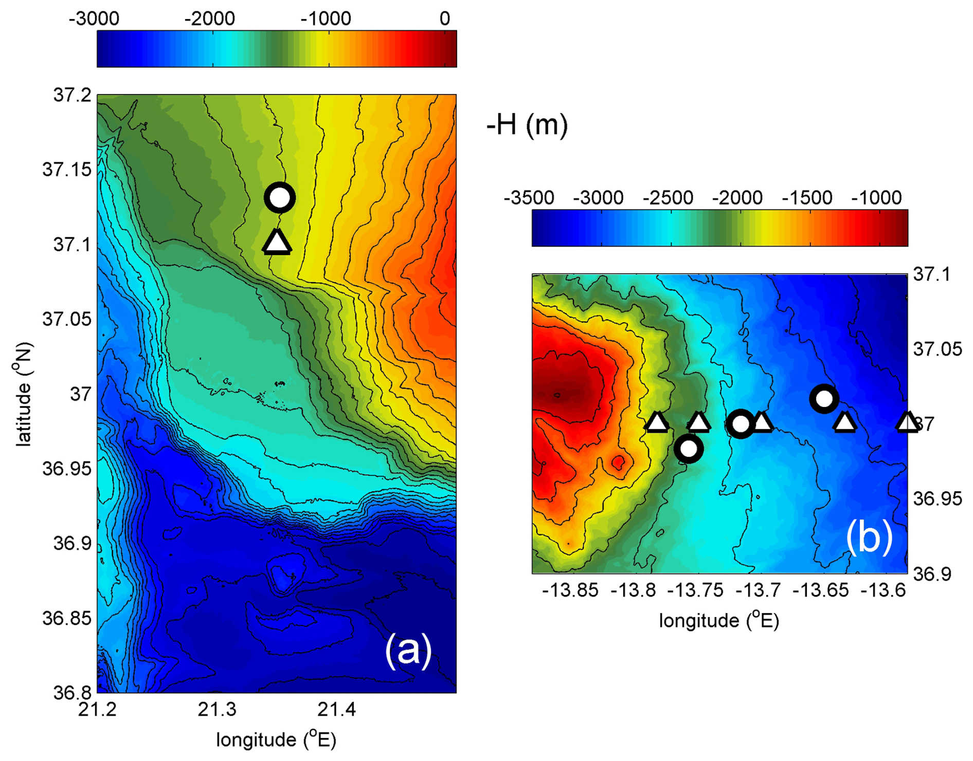
Figure 2 Two detailed maps made by the shipborne multibeam echo sounder. (a) Part of the western Peloponnese continental slope, Greece, eastern Mediterranean Sea, from R/V Meteor. The circle indicates the moored T-sensor location, and the triangle indicates the yo-yo CTD station. Black contours are drawn every 100 m. (b) Part of the eastern slope of Mount Josephine, northeastern Atlantic Ocean, from R/V Pelagia. The circles indicate the moored T-sensor locations, and the triangles indicate CTD stations during various years. Black contours are drawn every 250 m.

Although the multibeam echo sounder surveys were only a supporting part of the research cruises and therefore do not cover large areas, their extent is sufficient to resolve all internal wave scales. As a bonus, multibeam data processing also provides information on the reflective properties of the substrate for acoustic backscatter strength. This information was used by van Haren et al. (2015) to demonstrate that, over Mount Josephine, hard substrates consisting of coarse grain sizes and/or compacted sediment were almost exclusively found in areas with seafloor slopes that were supercritical for semidiurnal internal tides. Less reflective soft substrates consisting of fine grain sizes and/or water-rich sediment were found at subcritical slopes.

The x–y 2D gridded (essentially 3D with z included) seafloor elevation data from the above sources will be investigated spectrally for comparison with the 1D single-track (essentially 2D with z included) data from the northeastern Pacific hills explored by Bell (1975a, b). Some slope statistics are also pursued after computation of the proper slopes at all of the 2D gridded data points to characterize the ratio (percentage) of slopes exceeding a particular value. From the total number n_tot of 2D gridded data points per area, we calculate for a particular seafloor slope angle value γ_n the “ratio slope occurrence” $n/n_{\text{tot}}$ of the number n of slopes for which γ>γ_n. Its distribution will be compared with that of the theoretical internal wave, in this case the semidiurnal internal tide, characteristics (Eqs. 1 and 2) as a function of N in Sect. 4. A distribution of the measured N and these measured internal wave characteristics at all seafloor data points is impossible, also because of the natural variability as outlined in Sect. 2.3.

3.3 Analysis methods

Excursion length,

$$\begin{array}{}\text{(7)}& L_{\mathrm{e}}=UT/\mathit{\pi },\end{array}$$

is induced by oscillatory particle velocities $U\sin (\mathrm{2}\mathit{\pi }t/T)$ over time t, where U and T represent the flow speed and period, respectively. As the near-inertial wave period T_f varies with latitude, the two sites for detailed study demonstrate that

$$\begin{array}{}\text{(8)}& T_f\left(\right|\mathrm{37}\mathit{°}\left|\right)=\mathrm{1.8}{T}_{M\mathrm{2}}.\end{array}$$

As a result, for the given identical flow speed, the inertial excursion length will be 1.8 times that of the semidiurnal internal tide. Nonlinear waves may have different lengths. Excursion lengths will be compared with topography elevation spectra in Sect. 4.

As internal wave propagation depends strongly on N, for a given latitude and wave frequency, seafloor slope occurrence statistics should be compared with the ocean's volume-weighted stratification instead of using a vertically averaged N. For ocean volume V(z) per depth zone $[z+\mathrm{0.5}\mathrm{\Delta }z,z-\mathrm{0.5}\mathrm{\Delta }z]$ roughly every Δz=1000 m as defined in Costello et al. (2010, 2015), a volume-weighted buoyancy frequency N_v is calculated as

$$\begin{array}{}\text{(9)}& N_{\mathrm{v}}\left(z\right)=N\left(z\right)V\left(z\right)/\langle V\rangle ,\end{array}$$

where 〈…〉 denotes the averaging over the entire vertical water column.

4 Results

4.1 Vertical profiles

The shipborne water column CTD observations demonstrate moderately stratified and seldom homogeneous waters in the lower 300 m above the seafloor when N=N₁₀ is computed over small 10 m vertical scales (Fig. 3a). The variability with time is considerable, as can be inferred from the repeated CTD profiling over one inertial period. To get some idea of the variability of the layering in the ocean, N=N₁₀₀ 100 m profiles are given for comparison for different seafloor slopes and depths of the northeastern Atlantic area in Fig. 3b. Such variability in length-scale-dependent layering is similar in the lower 400 m above the seafloor of CTD profiles in the two areas, despite the considerable difference in seafloor depths.

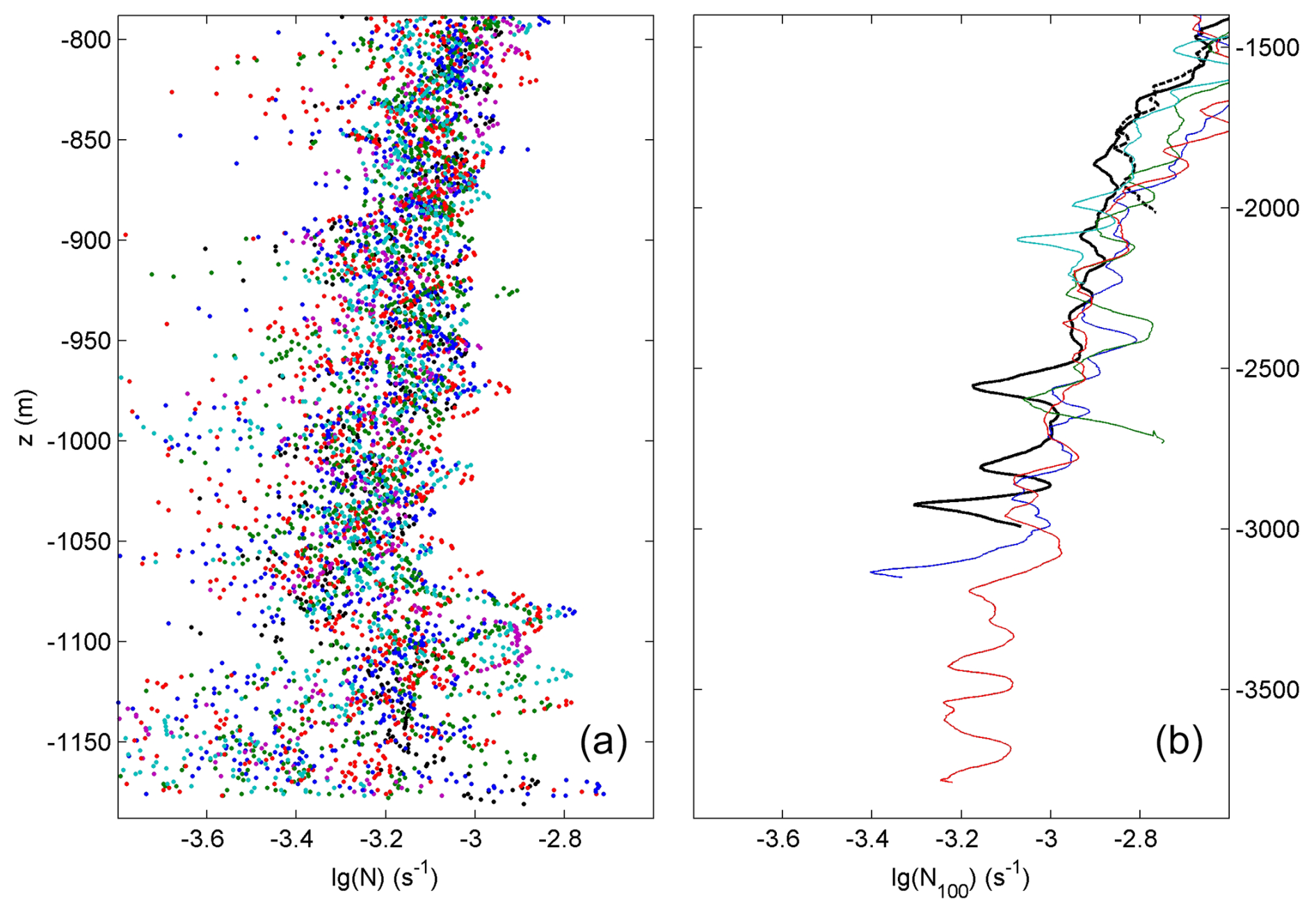
Figure 3 Logarithm base 10 (in mathematical notation) of the buoyancy frequency from the shipborne water column CTD. (a) One inertial period of 400 m yo-yo CTD hourly profiles, for 19 in total. Computations are made over 10 m vertical scales from a fixed location at H=1180 m water depth in the eastern Mediterranean. For clarity, the small-scale profiles are given by the colored dots. (b) Vertical range of 2500 m of the profiles from the area in van Haren et al. (2015). Computations are made over 100 m vertical scales down to 10 m from various seafloor depths and slopes on the eastern side of Mount Josephine in the northeastern Atlantic. The x axis scale is identical, but the y axis scale is different compared to panel (a).

In the lower 250 m above the seafloor of the eastern Mediterranean site, the variability in the N profiles becomes larger than in the interior above, with average values slowly decreasing with depth (Fig. 3a). This reflects larger internal wave breaking and re-stratification activity. In the lower 100 m above the seafloor, the variability in stratification is largest, both in the vertical and in time. The lower 400 m above the seafloor demonstrate averaged values of 〈N₁₀〉=7 ± $\mathrm{6}\times {\mathrm{10}}^{-\mathrm{4}}{\mathrm{s}}^{-\mathrm{1}}\approx \mathrm{8}f$, with a gradual decrease in values from 8 to $\mathrm{6}\times {\mathrm{10}}^{-\mathrm{4}}$ s⁻¹ towards the seafloor.

Similar mean N values are observed above Mount Josephine at 3 times greater depth. At H=3900 m, 〈N₁₀₀〉=7 ± $\mathrm{2}\times {\mathrm{10}}^{-\mathrm{4}}$ s⁻¹ is observed in the lower 400 m above the seafloor (Fig. 3b). The observed variations in N are about twice as high as sketched out in Sect. 2.2. At a given pressure level, however, the northeastern Atlantic site is about 0.5 orders of magnitude more stratified and 2 to 3 times larger in buoyancy frequency compared to the eastern Mediterranean and may thus support more internal wave energy and shear.

At the deepest northeastern Atlantic site considered here, whilst having the mean ocean water depth, the bottom slope is generally subcritical for internal tides (van Haren et al., 2015). This results from the gradual decrease in stratification with depth that leads to a steepening of internal wave characteristics following Eqs. (1) and (2), while the seafloor slope generally becomes smaller for concave topography. To become (super)critical for semidiurnal internal tides, the local slope would need to be (larger than) about 10°.

The (semidiurnal tidal) supercritical portion found above Mount Josephine in the interval $\mathrm{1000}<H<\mathrm{2300}$ m (van Haren et al., 2015) may be part of the 5 % of the surface area required to maintain the ocean stratification following ε_H. However, it is not sufficient on its own, as this required 5 % is larger than, albeit within 1 standard deviation from, the global total of 4 % surface area of the depth zone $\mathrm{1000}<H<\mathrm{2000}$ m (Costello et al., 2010, 2015). Because not all slopes between 1000 and 2000 m are expected to be supercritical (for semidiurnal internal tides, even under $N>\mathrm{2}\times {\mathrm{10}}^{-\mathrm{3}}$ s⁻¹; recall that basically all slopes are supercritical for particularly directed near-inertial waves), other supercritical slopes are sought. Supercritical slopes are more easily found at relatively shallow depths of 100–2300 m, given the statistically larger N and thus smaller internal wave slopes (Eqs. 1 and 2), resulting in sufficient turbulence caused by internal wave breaking.

How and where do internal waves shape the seafloor? Either the seafloor shape is concave and formed by erosion mid-slope, which, given the general mean stratification profile, leads to less likelihood of turbulent mixing due to internal wave breaking in the deep ocean, or it is convex through erosion above and below, which may favor deeper, supercritical slopes and associated enhanced stretches of mixing. Following nonlinear internal wave 2D modeling, no distinct difference in turbulence intensity is found between internal wave breaking at convex, concave, or planar slopes (Legg and Adcroft, 2003). However, their model results show relatively large values of energy dissipation at subcritical slopes, which are not found in ocean observations (e.g., van Haren et al., 2015). It is noted that the above modeling is based on 2D spatial shapes and that the ocean topography is essentially 3D, as in internal wave propagation and turbulence development. It is thus more generalizing to use full 3D seafloor elevation, i.e., full 2D slope statistics, and evaluate internal wave breaking with that. While near continental margins (where the continental shelf dives into the continental slope around H=200 m) the seafloor generally has a convex shape, it generally becomes concave at greater depths. Such topography would favor relatively shallow supercritical slopes (for semidiurnal internal waves).

4.2 Seafloor spectra

The multibeam echo sounder data (Fig. 2) allow for local seafloor investigations, in particular into scale size and slopes, that go beyond those of Bell (1975a, b), who used single-beam echo sounder data resolving height elevations at horizontal scales O(100) m, with a cutoff at a Nyquist wavenumber of about k_Nyq=2.5 cpkm. Bell (1975a, b) established a general seafloor elevation spectral falloff rate of kⁿ, $-\mathrm{2}<n<-\mathrm{5}/\mathrm{2}$ for $k_{\mathrm{0}}<k<k_{\text{Nyq}}$, with a smaller slope $-\mathrm{1}<n<\mathrm{0}$ for $k=k_{\mathrm{0}}<\mathrm{0.1}$ cpkm and a flattening n=0 for k<0.01 cpkm.

Our multibeam EMODnet and GEBCO datasets show a significantly steeper general falloff rate in elevation spectra (Figs. 4a and 5a) than in Bell (1975a, b), with dominant low-wavenumber falloff at a rate of about k⁻³ and saturation of noise values for k>10 cpkm. The steeper spectral falloff rates may be interpreted as a deviation from random distribution of seafloor elevation, in which energy is no longer distributed uniformly but is favored on the low-wavenumber side and reduced on the high-wavenumber side. It has an intermittent appearance (Schuster, 1984).

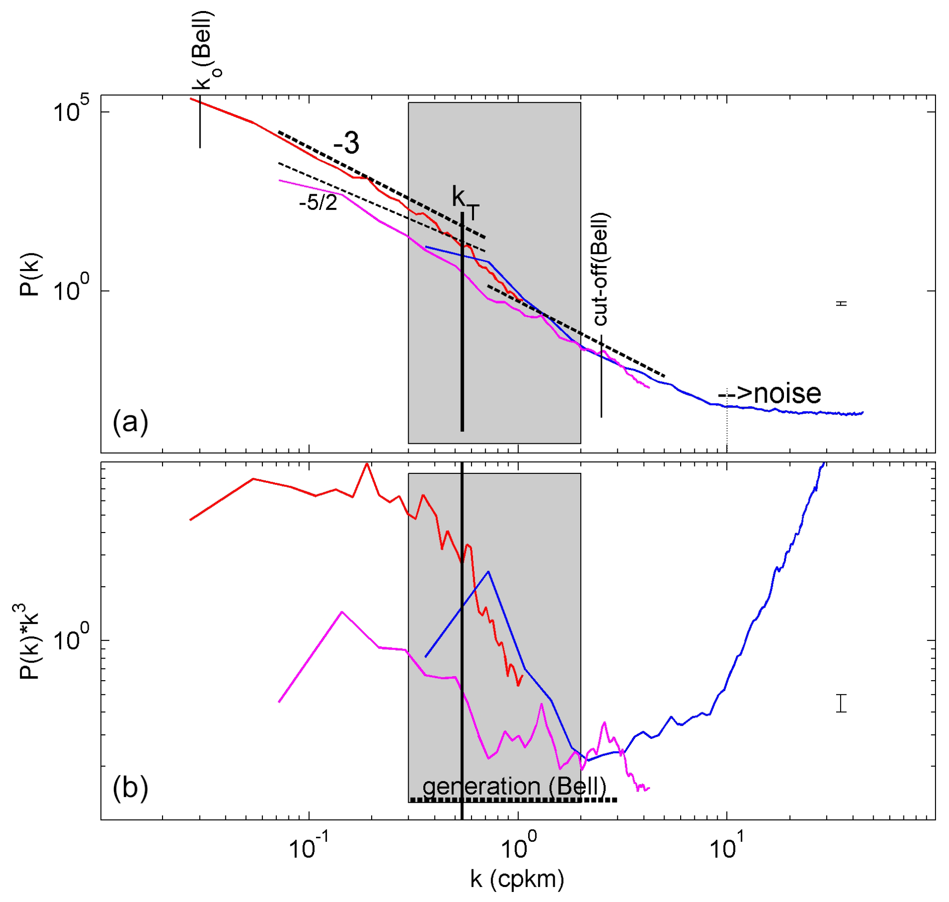
Figure 4 Spectral analysis of seafloor elevation as a function of the horizontal wavenumber k (the inverse of the horizontal length scale L). (a) On the log–log plot matching k⁻³ (−3 on the log–log plot), spectral slopes are represented by straight lines, with $k^{-\mathrm{5}/\mathrm{2}}$ ($-\mathrm{5}/\mathrm{2}$) being the slope reported by Bell (1975a). Bell's low-wavenumber cutoff k₀ is indicated, albeit barely resolved, as well as high-wavenumber roll-off to noise. The central vertical line at transient wavenumber k_T indicates a wavelength of 1852 m (1^′ in latitude). The three spectra are for the eastern Mediterranean averages in Fig. 2a: ${\mathrm{0.375}}^{\prime \prime }=\mathrm{11}$ m sampled multibeam data (blue), ${\mathrm{3.75}}^{\prime \prime }=\mathrm{115}$ m sampled EMODnet data (magenta), and ${\mathrm{15}}^{\prime \prime }=\mathrm{463}$ m sampled GEBCO data (red). The grey shading indicates the steep-slope range in which $n<-\mathrm{3}$ for kⁿ. (b) Same as panel (a) but for spectra scaled with k⁻³, the dominant low-wavenumber slope. The Bell (1975a, b) 1-decade range of internal wave generation of Pacific abyssal hills is indicated.

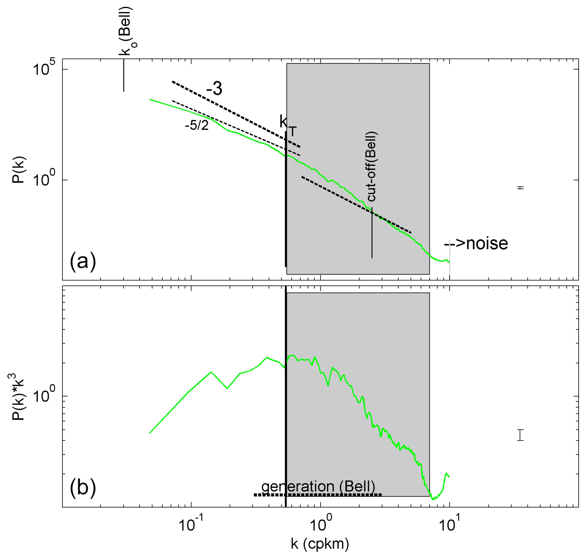
Figure 5 As in Fig. 4 but for the ${\mathrm{1.6}}^{\prime \prime }=\mathrm{49}$ m sampled Mount Josephine (northeastern Atlantic) multibeam data averaged in Fig. 2b. All of the straight lines are the same as in Fig. 4, but the shaded area is not.

In detail, the range $\sim \mathrm{0.3}<k<\sim \mathrm{2}$ cpkm shows the steepest falloff rates kⁿ, $n<-\mathrm{3}$ in the eastern Mediterranean (Fig. 4), and there are extended steep slopes in the interval $\sim \mathrm{0.55}<k<\sim \mathrm{6}$ cpkm in the northeastern Atlantic (Fig. 5). The shift from a steep slope range to higher wavenumbers in the northeastern Atlantic area corresponds approximately to the shorter excursion lengths for semidiurnal tides compared with inertial waves when following Eqs. (7) and (8) for the same flow speeds. The roll-off to weaker slopes for low wavenumbers is barely resolved, although the spectra do show the same tendency as in Bell (1975a, b). Extended GEBCO_2023 data across the Mid-Atlantic Ridge do resolve and show the roll-off at low wavenumbers (not shown).

The steepest falloff rate is most clearly visible after scaling the spectra with k⁻³ in Figs. 4b and 5b to better indicate this slump-down in seafloor elevation. Noting that this slump-down does not indicate a spectral gap, the observed range of strong (steeper) deviation before resuming $n=-\mathrm{2.5}$ or −3 centers around the “transition wavenumber” k_T≈0.5 cpkm, i.e., a wavelength of L_T≈2 km. It lies in the range of elevation variance spread that is visible in the data of Bell (1975a, b) and that overlaps the range of internal wave generation in the abyssal northeastern Pacific.

k_T is an indicator of a loss of seafloor topography variance at wavenumber k>k_T by about 1 order of magnitude, measuring the wavenumber range between the two $n=-\mathrm{3}$ spectral slopes in Figs. 4 and 5. As k_T is associated with the largest internal wave (excursion) scales, one may speculate that the loss of slope elevation relative to the general falloff rate is mainly related to low-frequency internal waves, semidiurnal internal tides, or near-inertial waves with longer periods (Eq. 8) than the M₂ tides at $\left|\mathit{\phi }\right|=\mathrm{37}\mathit{°}$, and their erosive turbulence generation smoothens out topography sizes. The spectral slump-down around k_T is statistically significant. However, it also varies significantly between different sites, shifting about 0.5 orders of magnitude to higher wavenumbers at Mount Josephine. This may be related to the dominance of the 1.8 times longer excursion length (∼ inverse wavenumber) of near-inertial waves in the eastern Mediterranean for a fixed flow speed. Possibly, the excursion length of nonlinear breaking internal waves is different for each site and different with dominant wave frequencies, being inertial or tidal. Excursion length perhaps varies most with local flow speed in other areas. For general GEBCO_2023 data from across the Mid-Atlantic Ridge in comparison with our data, one also finds a strict k⁻³ spectral falloff rate, and the spectral slump-down shifts by 0.5 orders of magnitude to lower wavenumbers (not shown).

4.3 Slope statistics

The mean slope of the seafloor topography calculated by Bell (1975a, b) at >100 m scales is 3 ± 1°. In our two small areas around the same latitude (Fig. 2), the slope distribution varies with the length scale; at slopes >3°, the shorter the length scales, the steeper the slopes that are calculated (Fig. 6). The 3° slope is the median seafloor slope value for our small eastern Mediterranean site, irrespective of the scales used (Fig. 6a). The median seafloor slope value for our small northeastern Atlantic site varies per scale and is about 4° at 1^′ resolution and 5° at 0.25^′ resolution (Fig. 6b). These median slopes are found for the common mean N at $z>-\mathrm{2000}$ m.

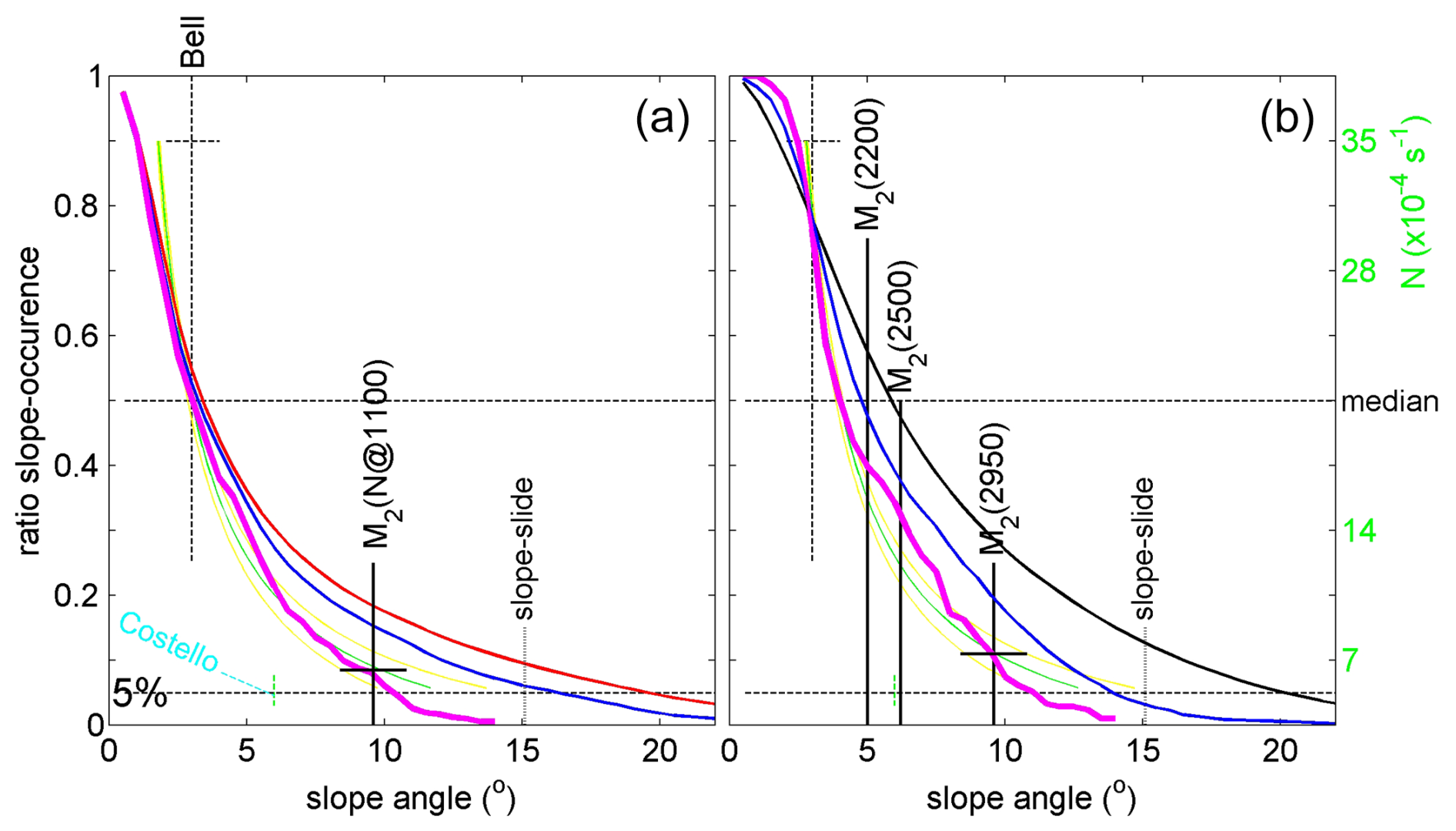
Figure 6 Seafloor statistical curves of the ratio of slope occurrence to the percentage of slopes larger than a particular slope angle (Sect. 3.2), for different seafloor elevation sampling scales. For comparison, graphs are plotted for theoretical M₂ internal tide characteristic slopes as a function of N, scale to the right, one in green using Eq. (1) and two in yellow using Eq. (2). The horizontal center dashed line indicates the median, and the lower horizontal dashed line indicates the 0.05 (5 %) level that is required for (just) supercritical slopes to generate sufficient global turbulence. The vertical black dashed lines indicate the Bell (1975b) average slope of northeastern Pacific abyssal hills and the maximum slope before collapse of sediment packing “slope slide”. (a) From the eastern Mediterranean map of Fig. 2a using three different scales for elevation slope computations: $L={\mathrm{1}}^{\prime }$ (magenta), 15^′′ (blue), and 3.75^′′ (red). The Costello et al. (2010) range of percentages is indicated in light blue (see the text). The semidiurnal lunar (M₂) internal tide slope is indicated for the local N at H=1100 m, with a corresponding error spread in characteristic values. (b) From the northeastern Atlantic map of Fig. 2b using $L={\mathrm{1}}^{\prime }$ (magenta), 14.5^′′ (blue), and 1.6^′′ (black). The M₂ slopes for the three different mooring sites are indicated as a function of their H (m).

For most of the global ocean using 1^′ resolution, Costello et al. (2010) found that 9.4 % of the seafloors have a slope between 2 and 4°, 8.2 % have a slope >4°, and 4.5 % have a slope >6°, from which we conclude that 3.7 % have a slope between 4 and 6°. Recall that 75 % of the ocean area and 90 % of its volume have seafloors between 3000 and 6000 m, where most of these slope percentages are. From the slope statistics of Costello et al. (2010), it is noted that the mean and standard deviation values do not vary significantly in the interval $-\mathrm{7500}<z<-\mathrm{1500}$ m but are significantly lower and higher than the averages at $z>-\mathrm{1500}$ m and $z<-\mathrm{7500}$ m, respectively.

At our two sites, slopes are slightly steeper at 1^′ resolution, and 5 % of the seafloors have slopes >10° and are supercritical for semidiurnal tidal and thus also inertial frequencies for the local mean N. The statistical distribution of the semidiurnal internal tidal wave characteristic slope as a function of N follows that of seafloor slopes at 1^′ resolution. For the eastern Mediterranean, at 1^′ resolution the (semidiurnal tidal) critical slope is 9.6° for the local $N=\mathrm{6.6}\times {\mathrm{10}}^{-\mathrm{4}}$ s⁻¹, from which it is concluded that, statistically, (just over) 5 % of the slopes are supercritical for M₂. This value of N is to within an error the same value found for N_v found for N_v after volume-weighted averaging from Eq. (9) for $z<-\mathrm{500}$ m of open northeastern Atlantic and Mariana Trench (Pacific Ocean) CTD observations by van Haren et al. (2017, 2021) (Fig. 7). It is noted that this volume-weighted averaging includes effects of Antarctic Bottom Water, as observed in the Mariana Trench profile. The value of N_v is 3 times smaller than the mean buoyancy frequency used by Cacchione et al. (2002).

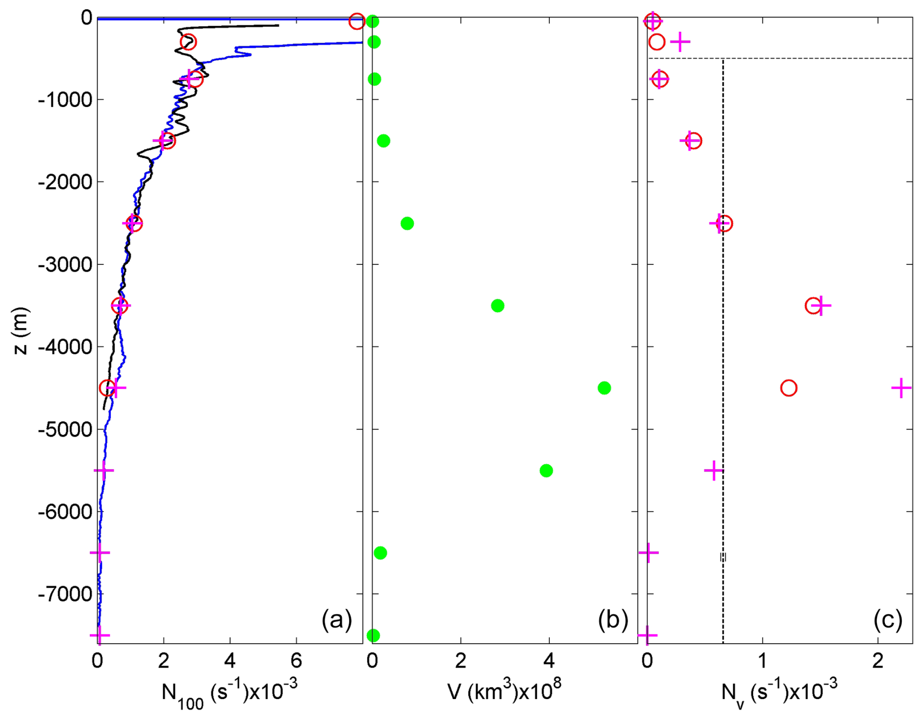
Figure 7 Weighted function of buoyancy frequency as a function of the vertical. (a) Large 100 m buoyancy frequency from the northeastern Atlantic off Mount Josephine (black profile with red circles) from the area in van Haren et al. (2015) and over and inside the Mariana Trench (blue with magenta plus signs) in van Haren et al. (2017, 2021). (b) Ocean volume V(z) per depth zone, adapted from Costello et al. (2010) with depth zones defined in Costello et al. (2015). (c) Volume-weighted values of buoyancy frequency in panel (a) following Eq. (9) using V(z) in panel (b). Note the relatively large value from around −4500 m in the Mariana Trench data that is associated with Antarctic Bottom Water. Below $z<-\mathrm{500}$ m, the vertical dashed line indicates the mean value 〈N_v〉=6.6 ± $\mathrm{0.2}\times {\mathrm{10}}^{-\mathrm{4}}$ s⁻¹ for both profiles, with a small error bar.

At this volume-weighted average N_v, the associated supercritical slopes for semidiurnal lunar internal tides are found to occur for 5 % of all of the slope values; i.e., 5 % of all of the slopes are >9.6° (Fig. 6a). This percentage is reached at an angle of 20° for the 1.6^′′ multibeam data of Mount Josephine (Fig. 6b). As this angle value is steeper than that for sedimentary stability, its seafloor texture may foremost consist of hard substrate, which indeed has been observed in multibeam data for supercritical slopes (van Haren et al., 2015).

However, when computed at the higher 1^′ resolution (magenta lines in Fig. 6), one finds a 5 % transition for 11°, which is to within error the same slope for the northeastern Atlantic and eastern Mediterranean multibeam data. Thus, seafloor slope statistics are identical to within an error between our two sites at 1^′ resolution. Recall that the 1^′ resolution is close to the spectral transition length scale $\mathrm{1}/k_{\mathrm{T}}$ (Figs. 4 and 5) and close to the longest internal wave excursion length for typical deep-sea flow speeds. The characteristic (Eq. 2) slope range between 9 and 11° comprises the 10° seafloor slope above which semidiurnal internal tides become supercritical at sites of the 3900 m mean ocean water depth given the local N. Although this N is found around 1100 m in the eastern Mediterranean, the approximately 2.5 times weaker N, compared with the northeastern Atlantic data at the same depth, is associated with small tides, so that the inertial energy is about 40 % of the total (inertial and tidal) internal wave energy found in the northeastern Atlantic.

Although volume-weighted mean N_v and thus mean internal tidal characteristic slopes are found in the depth zone of the mean ocean depth comprising 75 % of the ocean area (Costello et al., 2010), the occurrence of 5 % supercritical slopes reduces local relatively weak turbulence dissipation rates O(10⁻⁹) m² s⁻³ to a small contribution of <10 % to maintain global ocean stratification. However, the coincidence of 5 % seafloor slopes with supercritical slopes for the volume-weighted mean N and N at the mean ocean depth may reflect an ocean-wide balance of internal wave turbulence and topography interaction. Locally in the deep sea, such turbulence may have considerable influence on the redistribution of sediment and nutrients. Examples are short-term contributions of inertial waves generated by, e.g., large storms such as typhoons. For the standard mean 10⁻⁸ m² s⁻³ over h=200 m in H=3900 m, 5 % semidiurnal tidal supercritical slopes yield a global contribution of $\mathrm{2.5}\times {\mathrm{10}}^{-\mathrm{11}}$ m² s⁻³. A passing typhoon may dissipate 10⁻⁷ m² s⁻³, as observed (van Haren et al., 2020) over h=200 m in H=3100 m at any slope, as all slopes are basically supercritical for a near-inertial wave characteristic.

Considering the more numerous moored T-sensor observations from the depth zone 100–2000 m (Fig. 1), which comprises 10 % of the ocean area (Costello et al., 2010, 2015), the larger local N shows 50 % of the local slopes to be supercritical (for semidiurnal tides) (see Fig. 6b). The overall 50 % of 10 % = 5 % supercritical slopes are sufficient for maintaining the entire ocean stratification over a typical h=100 m in average H=1000 m and an observed turbulence dissipation rate ${\mathit{\epsilon }}_{h_{\mathrm{o}}}$. This is also the depth zone in which cold-water corals (CWCs) thrive (United Nations, 2017). The suspension feeding CWCs rely on nutrient supply by sufficiently turbulent hydrodynamic processes.

5 Discussion

Cacchione et al. (2002) made calculations with water level height mean N above a mean-depth ocean seafloor, holding the N value constant for all $z<-\mathrm{150}$ m. This does not represent a realistic internal wave turbulence environment, because (1) N monotonically decreases with depth (except under local conditions such as when Antarctic Bottom Water is found near 4000 m), (2) internal waves refract so that local N has to be accounted for, and (3) internal waves predominantly break at a sloping seafloor and not in the ocean interior.

It is well-established that internal tidal dissipation mainly occurs over steep topography (e.g., Jayne et al., 2004). However, these authors emphasize that global modeling efforts still lack a high-resolution bathymetry dataset to improve our ability to better quantify ocean mixing and understand its impact on Earth's climate. It may well take considerable effort and time until we have mapped the seafloor to the same detail as the surface of Mars (Smith, 2004).

Deep-ocean internal waves can be modeled to first order as linear waves and are ubiquitous throughout all seas and oceans. However, given their natural environment, which is not constant in space and time, and their potential interactions with other water flows, they diverge considerably from linear constant-frequency waves. First, the stratification support varies under internal wave straining, boundary flows, and (sub)mesoscale eddies, so that N shows a typical relative variation of ±20 %. Although semidiurnal internal tides are dominant energetically, their variation in frequency alone provides 6 % variations in the slopes of characteristics. In the deep sea, roughly the deeper half of all oceans, N<8f at mid-latitudes and full internal wave equations show a spread in internal tide characteristics of >15 %. All of these natural variations, not counting variations in seafloor slope determination as a function of length scale, provide a relative error range of the dominant internal wave characteristics of 25 %–50 %.

It thus seems impossible to find a particular persistent critical slope for a given single-internal wave frequency on a 1^′ scale that also ignores the highly nonlinear character of dominant turbulence-generating upslope-propagating bores, which are composed of motions at many internal wave frequencies. Therefore, it is not surprising that most internal-wave-generated turbulence occurs at (just) supercritical slopes, which provides a broader slope and thus frequency range.

As the above relative uncertainty range of internal wave characteristics matches that of a relative error of about 33 % (factor of 2) in mean turbulence dissipation rates, it reflects the uncertainty in determining present-day percentages of the supercritical slopes required to maintain ocean stratification, i.e., 5 % ± 1.5 % for seas where internal tides dominate. This uncertainty also sets the bounds for robustness of the internal wave–topography interactions: it is the margin within which variations are expected to find sufficient feedback not to disrupt the system from some equilibrium.

If so, spiking any variations in this system must go beyond an energy variation of about 30 %, which is larger than (the determination of) tidal variation but probably less than inertial motion variations, say wind (Wunsch and Ferrari, 2004). In terms of stratification, 30 % variation is feasible near the sea surface via seasonal and day–night variations, but this easily exceeds any natural stratification variations in the deep sea, say for $z<-\mathrm{500}$ m.

Suppose we can go beyond 30 % variation: what will happen then? It takes at least decades, centuries, or millennia for the seafloor elevation to adapt to an equilibrium of sufficiently supercritical slopes. If N increases uniformly by >30 % throughout the ocean, more (higher-frequency) internal waves will be supported and internal tide characteristics will become flatter. As a result, more (unaltered) seafloor slopes will become supercritical, which will raise the amount of ocean turbulence, perhaps by >30 %. Increased turbulence means more heat transport, hence a reduction in N that diminishes the initial 30 % increase. It goes without saying that the opposite occurs in the event of a decrease in N.

Although meager proof, we recall that the eastern Mediterranean deep sea has a factor of 2–3 times weaker N than the tidally dominated northeastern Atlantic Ocean at any given depth. This factor is commensurate with the 2–3 times weaker near-inertial internal wave energy compared with that of the combined energy of internal-tide and near-inertial waves. Both sea areas are in present-day equilibrium. As a result, it seems that it is not the buoyancy (density stratification) variations that strongly disturb the equilibrium, but the external sources of internal wave (kinetic energy).

Just supercritical slopes are probably bounded by a maximum of 15° for sedimentary slope instability. At any rate, the supercritical seafloor slopes allow development of upslope-propagating bores and rapid re-stratification of the back-and-forth sloshing internal tides. In contrast to forward wave breaking at a beach, internal tides break backwards at a slope (van Haren and Gostiaux, 2012b). This may explain the lack of a clear swash; i.e., while upslope-propagating bores may be considered an uprush, a clear vigorous backwash is not observed during the downslope warming tidal phase near the seafloor in moored T-sensor data. This demonstrates a discrepancy with the 2D modeling of Winters (2015). While in the model most intense turbulence is found near the seafloor during the downslope-phase expulsion into the interior, ocean observations demonstrate the highest turbulence around the upslope-propagating backward-breaking bore, with the bore sweeping material up from the seafloor (Hosegood et al., 2004). Some 3D or rotational aspect is probably important for ocean-internal wave breaking but has yet to be modeled.

We have considered a combination of seafloor elevation and internal wave turbulence data to revisit the interaction between topography and water flows in the deep sea. From various perspectives, including turbulence values, vertical density stratification, (water) depth zones, seafloor and internal wave slopes, and scale lengths, we have found that the interaction is relatively stable, where mainly internal tides and near-inertial waves shape the topography to within 30 % variability.

6 Conclusions

The median value of the seafloor slope of 3 ± 0.2° from multibeam echo sounder and satellite data from the northeastern Atlantic, mid-Atlantic Ridge, and eastern Mediterranean sites closely matches the rms-mean slope of 3 ± 1° established half a century ago from single-beam echo sounder data across northeastern Pacific abyssal hills (Bell, 1975a, b). Our result is found to be only weakly dependent on the scale, which we varied between 0.027^′ and 1^′. It lends some robustness to the determination of seafloor slopes for horizontal scales that match dominant internal wave excursion lengths.

The average spectral falloff rate of the seafloor elevation is found to be steeper than in Bell (1975a, b), which indicates a nonuniform distribution of scales instead of a uniform distribution as suggested previously. In particular, the spectral slump-down around a length scale of 2 km is noted, which suggests a lack of seafloor elevation shaped by the longest internal wave excursion length dissipating its energy into turbulence-creating sediment erosion. This spectral slump-down is found in seafloor elevation data from the northeastern Atlantic, where semidiurnal internal tides prevail, and at somewhat smaller values from the eastern Mediterranean, where tides are small and near-inertial motions that have 1.8 times larger length scales dominate internal waves. In the eastern Mediterranean, the buoyancy frequency is found to be smaller than at the corresponding depths in the northeastern Atlantic, which is commensurate with the contribution of internal tides (and the lack thereof).

Recent moored high-resolution T-sensor data (van Haren and Gostiaux, 2012a; van Haren et al., 2015, 2020, 2022, 2024; van Haren and Puig, 2017) demonstrated that internal wave breaking is found to be most vigorous above seafloor slopes that are supercritical rather than much more limiting, critical for (semidiurnal) internal tides, with a local turbulence dissipation rate of $>{\mathrm{10}}^{-\mathrm{7}}$ m² s⁻³ in the depth zone $\mathrm{100}<H<\mathrm{2200}$ m (northeastern Atlantic). This depth zone hosts most of the cold-water corals that depend on vigorous turbulence for nutrient supply. Our seafloor statistics show that 50 % of the slopes are supercritical for stratification in this depth zone, which compensates for the depth zone's occupation of only 10 % of the ocean area. As a result, we find that internal wave breaking at 5 % ± 1.5 % of all of the seafloor slopes suffices to maintain global ocean density stratification.

In zones of greater depth, internal wave breaking is generally less turbulent, contributing <10 % to maintain the global stratification, which is mainly due to steeper internal tidal characteristic slopes. Even in the deep sea, however, 5 % of the seafloor slopes coincide with supercritical slopes for the volume-weighted mean N_v and N at the mean ocean depth, supporting an ocean-wide balance of topography and internal wave turbulence interaction. Turbulence may be locally important for the redistribution of heat, nutrients, and oxygen, e.g., during the passage of typhoons generating near-inertial waves, as most seafloor slopes are supercritical for (one characteristic of) such waves, also in zones of great depth.