Coupling ocean currents and waves for seamless cross-scale modeling during Medicane Ianos

This study investigates the effects of a two-way wave–circulation coupled modeling framework during extreme weather events, with a particular focus on Medicane Ianos, one of the most intense cyclones to have occurred in the Mediterranean Sea. By utilizing a high-resolution unstructured numerical grid, the study explores wave–current interactions in both open-ocean and coastal environments. To this scope, we developed the first external coupler dealing with the SHYFEM-MPI circulation model and the WAVEWATCH III wave model. The interactions considered in this framework include sea-state-dependent momentum flux, radiation stress, Doppler shift, dynamic water depth for waves, and effective wind speed. The study adopts a rigorous validation of the formulations using idealized benchmarks tailored for these specific processes. Afterwards, the modeling framework was employed in real-case simulations of Medicane Ianos. The model is calibrated, and the ocean variables are rigorously validated against in situ and Earth observation (EO) data, including satellite-based measurements. The study found that wave-induced surge components contribute from 10 % to 30 % of the total water level during the storm and that sea-state-dependent momentum flux during a medicane can influence the vertical structure of the ocean up to 100 m. The accuracy of the wave model improves by around 3 % in terms of RMSE when coupled with a circulation model.

This study underscores the importance of such coupled models in accurately forecasting medicanes, storm surges, and their impacts, particularly as climate change intensifies extreme events in the Mediterranean Sea.

1 Introduction

Advanced knowledge on surface wind-driven gravity waves and currents and their interactions in the ocean is of great relevance to many decision support systems, such as metocean forecasting, early warning for storm surge events, oil spill evolution, search and rescue, beach erosion, and site choices for offshore infrastructures (Hashemi and Neill, 2014). Physically, the surface gravity waves can affect the vertical mixing, as well as surface and bottom stresses experienced by currents. Surface waves and currents can also exchange energy through the concept of radiation stress (Longuet-Higgins and Stewart, 1961; Mellor, 2003) or vortex force (VF) (Ardhuin et al., 2008; McWilliams et al., 2004). In return, ocean currents can modify the relative speed of the air above the sea surface (relative wind effect) and change the absolute frequency of waves due to the Doppler shift. Spatial variability of currents can modify the relative wave frequency and cause wave refraction, shoaling, and breaking that mimic bathymetric effects.

An accurate computation of total water level (TWL) during storm surge events combining multiple drivers (e.g., surges, tides, waves) becomes relevant to forecast flooding and impacts in coastal and urban areas. Kim et al. (2008) used a coupled surge–wave–tide (SuWAT) model to demonstrate that high tides can mitigate storm surges. Their study highlighted the relationship between locally generated surge and wave setup with the tidal state. They emphasized that considering surges, waves, and tides independently can lead to an overestimation of TWL. Additionally, they underscored the importance of incorporating bottom friction, wind–wave interactions, and wave–current interactions for more accurate storm surge estimations. Continuing the development, with the focus on the effects of wind stress parameterizations and wave-induced radiation stress on storm surge, Kim et al. (2010) estimated 40 % contribution of radiation stresses to the peak sea level rise.

Jo et al. (2024) studied the typhoon-caused inundations concluding that uncoupled models overestimate wave-overtopping peak discharge by 8 %. Hsiao et al. (2019) used fully coupled circulation–wave model (SCHISM + WW3) to simulate super typhoon events. They observed that surface waves, especially wave setups, exhibited the most significant nonlinear interaction with storm tides, while wave–tide interaction was relatively minor. Dietrich et al. (2011) coupled a shallow-water model (ADCIRC) with the wave model SWAN, utilizing the same unstructured grid to simulate the waves and storm surges induced by the hurricanes Katrina and Rita in the Gulf of Mexico. The model demonstrated that as Hurricane Katrina moved onto the continental shelf, depth-limited breaking waves exerted stresses on the water column, increasing overall water levels by 0.2–0.3 m and driving currents, contributing up to 35 % of the TWL and 10 % of overall currents in the region.

Extreme meteorological events are intensifying in the Mediterranean Sea due to climate changes; among these we have the Mediterranean tropical-like cyclones or medicanes (Cavicchia et al., 2014; Sánchez-Arcilla et al., 2016). Medicanes are rare meteorological phenomena that exhibit characteristics similar to tropical cyclones, such as a warm core, eye formation, and strong winds. These systems, however, form and evolve under the unique conditions of the Mediterranean Sea, typically during the autumn and early winter months when sea surface temperatures are sufficiently warm to support their development (Cavicchia et al., 2014). Although medicanes are generally less intense and shorter-lived compared to their tropical counterparts, they can still cause significant damage and pose considerable risks to the regions they affect. Notable examples include Medicane Rolf in 2011 and Medicane Zorbas in 2018, both of which provided valuable insights into the dynamics and impacts of these systems (Flaounas et al., 2022). Among the most harmful recent medicanes is Medicane Ianos, which struck Greece in September 2020, causing widespread damages, exceeding USD 700 million and resulting in human casualties (Diakakis et al., 2023). The study of medicanes is crucial for advancing our understanding of these phenomena and enhancing preparedness and response strategies in the Mediterranean region (Ferrarin et al., 2023).

This study aims to investigate the impact of a two-way coupled wave–circulation model on ocean dynamics during extreme events, with a focus on Medicane Ianos. Using very high-resolution and unstructured numerical grid, we describe the contribution of wave–current interaction during one of the most intense cyclones in the Mediterranean Sea.

We carried out this work using a new modeling framework based on SHYFEM-MPI (Micaletto et al., 2022; Verri et al., 2023) and a state-of-the-art community wave model WAVEWATCH III (hereafter WW3) (Tolman, 2009; WW3DG, 2019). For this study, an external Python-based coupler is developed to manage the mutual exchanges between the numerical cores, enabling two-way coupling.

The WW3 model is widely used by several organizations worldwide to simulate waves in various systems across different regions, ranging from global (Alday et al., 2021; Brus et al., 2021; Mentaschi et al., 2020) to regional (Abdolali et al., 2020; Causio et al., 2021, 2024) and coastal scales (Pillai et al., 2022a, b).

The SHYFEM model has previously been coupled with wave models, as in Roland et al. (2009). It serves as the circulation core of the storm surge early warning system Kassandra (Ferrarin et al., 2013) and has recently been employed to analyze uncertainties related to the simulation of the Medicane Ianos (Ferrarin et al., 2023). In these studies, they adopted a barotropic implementation, with the unstructured WWMIII wave model (Roland, 2009) integrated through hard coupling.

Present work incorporates new processes into the two-way coupling between SHYFEM–WW3, including the sea-state-dependent momentum flux and wind field correction based on the air stability parameter. The study marks the first study to implement a three-dimensional baroclinic version of the wave coupled SHYFEM model.

The reliability of the results and the code is validated using well-established idealized benchmarks and analytical results. Specifically, we use the planar beach (Xia et al., 2020) and the wave-tidal-driven inlet (Cobb and Blain, 2002).

Furthermore, this newly developed coupled system is applied to a real case, simulating the impacts of Medicane Ianos on ocean and wave fields, as well as their interactions, using a cross-scale unstructured-grid domain. This domain enables us to examine both (i) open-ocean features, such as sea surface cooling induced by Medicane Ianos, the impact of the coupling on vertical profiles, and the effects of circulation on large scale wave dynamics, and (ii) local coastal features, including TWL and wave contribution to storm surge.

The paper is structured as follows. Section 2 introduces the modeling framework, including the circulation and wave modeling suite as well as the coupling methodology. Section 3 validates the coupling procedure using idealized test cases. Section 4 investigates the medicane-induced effects on the ocean, with a specific focus on coastal storm surge. Finally, conclusions are provided in Sect. 5.

2 The modeling framework

This study is based on a coupled modeling framework built on WW3 and SHYFEM-MPI. Both models run on the same unstructured computational grid, a classic methodology in coupled unstructured modeling, used from early studies to the most recent ones, such as in Mentaschi et al. (2023). This avoids further interpolations, and it allows a seamless approach to address large-scale and coastal processes. Unstructured grids also ensure an accurate representation of both natural and artificial irregular coastal features (Bertin et al., 2014), and it allows for high-resolution modeling along the coast.

2.1 Circulation modeling

The circulation model used in this study is SHYFEM (System of HydrodYnamic Finite Element Modules), a 3D baroclinic finite-element hydrodynamic model (Federico et al., 2017; Umgiesser et al., 2004; Verri et al., 2023) that solves the Navier–Stokes equations by applying the hydrostatic and Boussinesq approximations. The SHYFEM-MPI version, developed by the Centro Euro-Mediterraneo sui Cambiamenti Climatici (CMCC) (Micaletto et al., 2022), is used in this study and, for the first time, is coupled with the wave model WW3.

The model employs a semi-implicit algorithm for time integration, providing unconditional stability with respect to gravity waves, bottom friction, and Coriolis terms, thus allowing transport variables to be solved explicitly. The Coriolis term and pressure gradient in the momentum equation, along with the divergence terms in the continuity equation, are treated semi-implicitly. Bottom friction and vertical eddy viscosity are treated fully implicitly for stability reasons, while the remaining terms (advective and horizontal diffusion terms in the momentum equation) are treated explicitly. The finite-element discretization is applied on unstructured B-type grids. More detailed descriptions of the model equations and discretization methods are provided in Micaletto et al. (2022) and Verri et al. (2023).

In this work, we implemented the transport and diffusion equation for tracers, with horizontal and vertical advection values based on a total variation diminishing (TVD) scheme. An upwind scheme is employed to discretize the horizontal advection of momentum, and the Smagorinsky (1963) formulation is used to compute horizontal eddy viscosity. Vertical viscosities and diffusivities are calculated using a k–ε scheme adapted from the General Ocean Turbulence Model (GOTM) (Burchard and Petersen, 1999). Bottom stress is computed using the quadratic formulation with a bottom drag coefficient defined based on the logarithmic formulation and water depth. In the logarithmic formulation, the von Kármán constant is assigned a value of 0.4, and the bottom roughness length is 0.01.

The model has been successfully applied in operational (Federico et al., 2017) and relocatable forecasting systems (Trotta et al., 2021), storm surge events (Alessandri et al., 2023; Park et al., 2022), and as a part of a digital twin by Pillai et al. (2022b).

2.2 Wave modeling

The wave model used is WW3 v6.07, a third-generation wave modeling framework that incorporates the latest scientific advancements in wind–wave modeling and dynamics. Developed by the US National Centers for Environmental Prediction (NOAA/NCEP) and inspired by the WAM model (Komen et al., 1984), WW3 solves the random phase spectral action density balance equation for wavenumber–direction spectra. The model includes options for shallow-water (surf zone) applications and features numerical schemes capable of solving the propagation of a wave spectrum at high resolutions on unstructured (triangular) grids (Abdolali et al., 2020).

In this study, the wave energy spectra are discretized into 24 equally spaced directional bins covering the full circle and a 30 log-varying frequency discretization (0.05–0.7932 Hz). The source input and dissipation terms are based on the Source Term 4 (ST4, package T741) physics from Ardhuin et al. (2010). Non-linear wave–wave interactions are implemented using the discrete interaction approximation (DIA) from Hasselmann and Hasselmann (1985). Bottom friction is defined using the JONSWAP parameterization (Hasselmann et al., 1973), and depth-induced breaking follows the criterion described by Battjes and Janssen (1978) and Miche (1944) for defining the breaking threshold. Furthermore, we calibrated the wind–wave coupling parameter (BETAMAX = 1.43) to improve model results and reduce the underestimation of wave height. Nonlinear triad interactions are modeled using the Lumped Triad Approximation (LTA) model of Eldeberky (1996). The second-order propagation scheme Contour Residual Distribution–Positive Streamline Invariant (CRD-PSI) (Roland, 2009) is used to describe wave propagation with a global time step of 200 s.

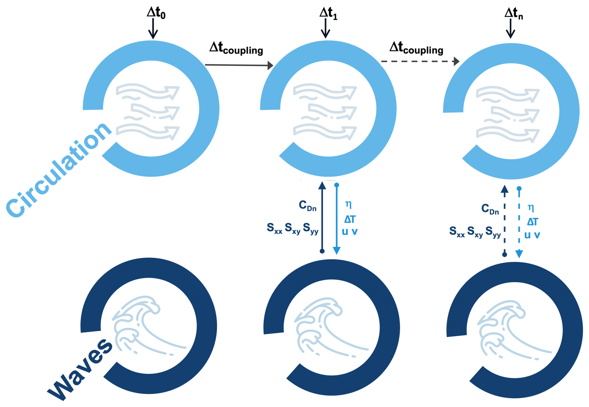
Figure 1 The coupling procedure between SHYFEM-MPI and WW3. When the simulation starts, models exchange information after the first time step (e.g., Δt₀ = 300 s) and then exchange every Δt_coupling (e.g., every 1 h). SHYFEM-MPI sends sea level (h), current fields (u,v), and air–sea temperature difference (ΔT) to WW3. WW3 sends neutral drag coefficient (C_Dn) and radiation stresses (S_xx, S_xy, S_yy) to SHYFEM-MPI.

2.3 Coupling methodology

The two-way interaction in the modeling framework is achieved via an external Python-based coupler, which has the advantage of using the native versions of the standalone models, thereby minimizing code changes. The primary changes applied to the native codes relate to new physical process inclusion.

For this study, multiple sensitivity tests are conducted to evaluate the system's response to the coupling frequency (Δt_coupling), identifying 1 h as an optimal balance between the exchange frequency and the computational performance. However, Δt_coupling is set to 30 min for the idealized test cases to be consistent with previous studies, while 1 h is used for the real case.

The main objective of this study is to characterize the wave-induced surge component in the total water level, with a focus on the effect of waves on circulation. This involves incorporating the theory of Longuet-Higgins and Stewart (1961). Additionally, to provide a more comprehensive set of interactions from coastal to large scale, we include sea-state-dependent momentum flux, based on the neutral drag coefficient, as described by Clementi et al. (2017). Conversely, to preserve the integrity of two-way interactions, the effect of circulation on waves is addressed by incorporating the Doppler shift induced by surface ocean currents, by dynamically updating the water depth based on the sea surface height and by correcting the wind field according to a stability parameter dependent on the air–sea temperature difference (Abdalla and Bidlot, 2002). This approach accounts for wind gustiness, which can enhance the representation of extreme conditions during storms (Abdalla and Cavaleri, 2002).

A schematic representation of the two-way coupling is shown in Fig. 1 and detailed below.

The circulation model receives the radiation stress components and the wind neutral drag coefficient computed by the wave model. The radiation stress components S_xx, S_xy, and S_yy account for wave transformation in coastal areas, resulting in a net flux of momentum. According to the Longuet-Higgins and Stewart (1962) theory, wave setup balances the shoreward gradient in radiation stress, with the sea surface pressure gradient counteracting the gradient of incoming momentum. The wave-induced momentum flux (F), derived by the gradients of the radiation stress, is estimated and included in the momentum equation (Eq. 1).

$$\begin{array}{}\text{(1)}& F={\displaystyle \frac{\mathrm{1}}{\mathit{\rho }}}\left({\displaystyle \frac{\partial S_{xx}}{\partial x}}+{\displaystyle \frac{\partial S_{xy}}{\partial y}},{\displaystyle \frac{\partial S_{xy}}{\partial x}}+{\displaystyle \frac{\partial S_{yy}}{\partial y}}\right)\end{array}$$

The sea-state-dependent wind stress involves exchanging the neutral drag coefficient from the WW3 wave model, following Clementi et al. (2017). This coefficient is computed using a formulation derived from the quasi-linear theory of wind–wave generation, as developed by Janssen (1989, 1991) and based on Miles (1957). According to this theory, the neutral drag coefficient (C_Dn) (Eq. 2) depends on the effective roughness length, which is influenced by the sea state through the wave-induced stress estimated from the wave spectra.

$$\begin{array}{}\text{(2)}& C_{\text{Dn}}={\left({\displaystyle \frac{\mathit{\kappa }}{\text{log}\left(\frac{z_{\mathrm{u}}}{z_{\mathrm{0}}}\right)}}\right)}^{\mathrm{2}},\end{array}$$

where z_u is the height of the wind forcing, κ =  0.4 is the von Kármán constant, and z₀ is the roughness length modified by the ratio of the wave-supported stress τ_w to the total stress τ, as in Eq. (3). τ_w represents the flux of momentum that is directly input into the wave field by the wind.

$$\begin{array}{}\text{(3)}& z_{\mathrm{0}}={\displaystyle \frac{{\mathit{\alpha }}_{\mathrm{0}}\mathit{\tau }}{\sqrt{\mathrm{1}-\frac{{\mathit{\tau }}_{\mathrm{w}}}{\mathit{\tau }}}}},\end{array}$$

where α₀ = 0.0095. The C_Dn is transferred to the circulation model for the estimation of the turbulent drag coefficient according to Large (2006).

The circulation interacts with the wave field through sea level, currents, and air–sea temperature difference. The sea level (η) allows for a dynamic adjustment (d) of the water depth (h) in the wave equations as in Eq. (4):

$$\begin{array}{}\text{(4)}& d=h+\mathit{\eta }.\end{array}$$

Ocean currents influence wave characteristics, including wavelength, amplitude, wavenumber, and direction. In the WW3 model, the Doppler shift accounts for the changes in wave frequency due to the relative motion between waves and currents, which can be expressed as in Eq. (5):

$$\begin{array}{}\text{(5)}& \mathit{\omega }=\mathit{\sigma }+\mathit{k}\cdot \mathit{U},\end{array}$$

where ω is absolute frequency, σ is relative frequency, k is vector of wave number, and U is current velocity.

The stability of the atmosphere is influenced by the air–sea temperature difference (ΔT). Tolman (2002), inspired by the work of Abdalla and Bidlot (2002), formulated a stability correction replacing the wind speed in WW3 with an effective wind speed, ensuring that the wave growth corresponds to both stable and unstable wave growth patterns. The ΔT defines a stability parameter according to Eq. (6):

$$\begin{array}{}\text{(6)}& \text{ST}={\displaystyle \frac{hg}{U_z^{\mathrm{2}}}}{\displaystyle \frac{\mathrm{\Delta }T}{T_{\mathrm{0}}}},\end{array}$$

where U_z is wind speed at height z, ΔT is the air–sea temperature difference, and T₀ is the reference temperature. ST is used to compute effective wind speed, U_e (Eq. 7):

$$\begin{array}{}\text{(7)}& U_{\mathrm{e}}=U_{\mathrm{10}}{\left({\displaystyle \frac{c_{\mathrm{0}}}{\mathrm{1}\pm c_{\mathrm{1}}\text{tanh}\left[c_{\mathrm{2}}\right(ST-{\text{ST}}_{\mathrm{0}}\left)\right]}}\right)}^{\frac{\mathrm{1}}{\mathrm{2}}},\end{array}$$

where U₁₀ is wind speed at 10 m, c₀ is 1.4, c₁ is 0.1, c₂ is 150, and ST₀ is  −0.0.1.

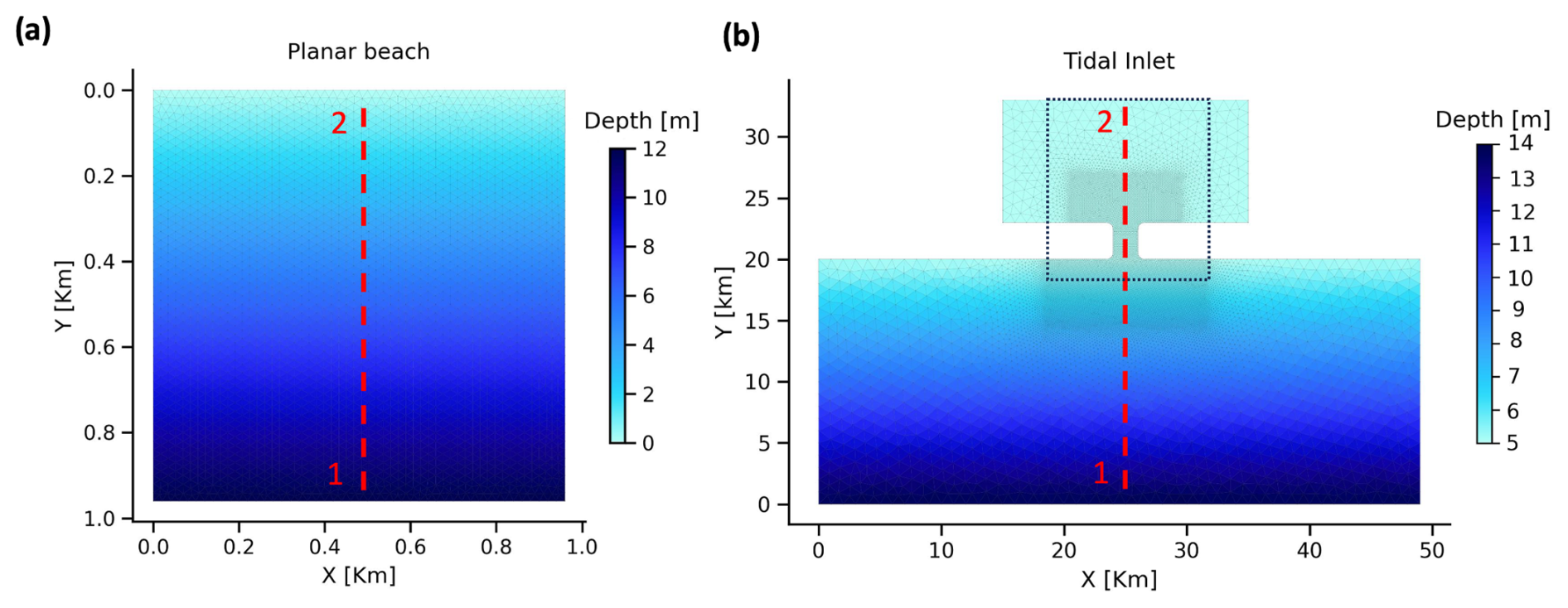
Figure 2 Numerical domain and bathymetry of the two idealized benchmarks: the planar beach (a) and the tidal inlet (b). Dashed red lines show the transect from point 1 to point 2, where the numerical solutions were assessed. The dotted box in (b) denotes the area magnified and is shown later in the “Results” section.

3 Validation of the coupling strategy with idealized test cases

The robustness of the two-way coupling and its physics is assessed and evaluated through idealized numerical experiments. The test cases selected for this assessment include two common benchmarks for the wave–current interaction at coastal scale: a planar beach (Fig. 2a) from Xia et al. (2020) and an idealized tidal inlet (Fig. 2b) from Cobb and Blain (2002).

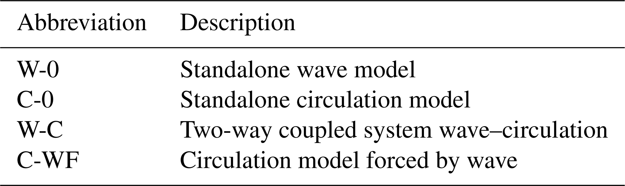
Table 1 lists the abbreviations of the simulations used for the validation of the idealized test cases.

Table 1 Configurations and nomenclature for the numerical setup used in this study.

3.1 The planar beach

The planar beach is used in this work for assessing the wave setup/setdown along transect 1–2 (Fig. 2a). The results obtained from our numerical model are compared with the analytical solution as described in Xia et al. (2004), to validate the accuracy and reliability of the implementation in modeling wave contributions to the surge, ensuring that the modeled outcomes are consistent with the theoretical solution. The validation is carried out utilizing the C-WF configuration, where the wave model exclusively provides inputs (forcing fields) to the circulation model. This setup allows the model to reach a semi-stationary condition more quickly.

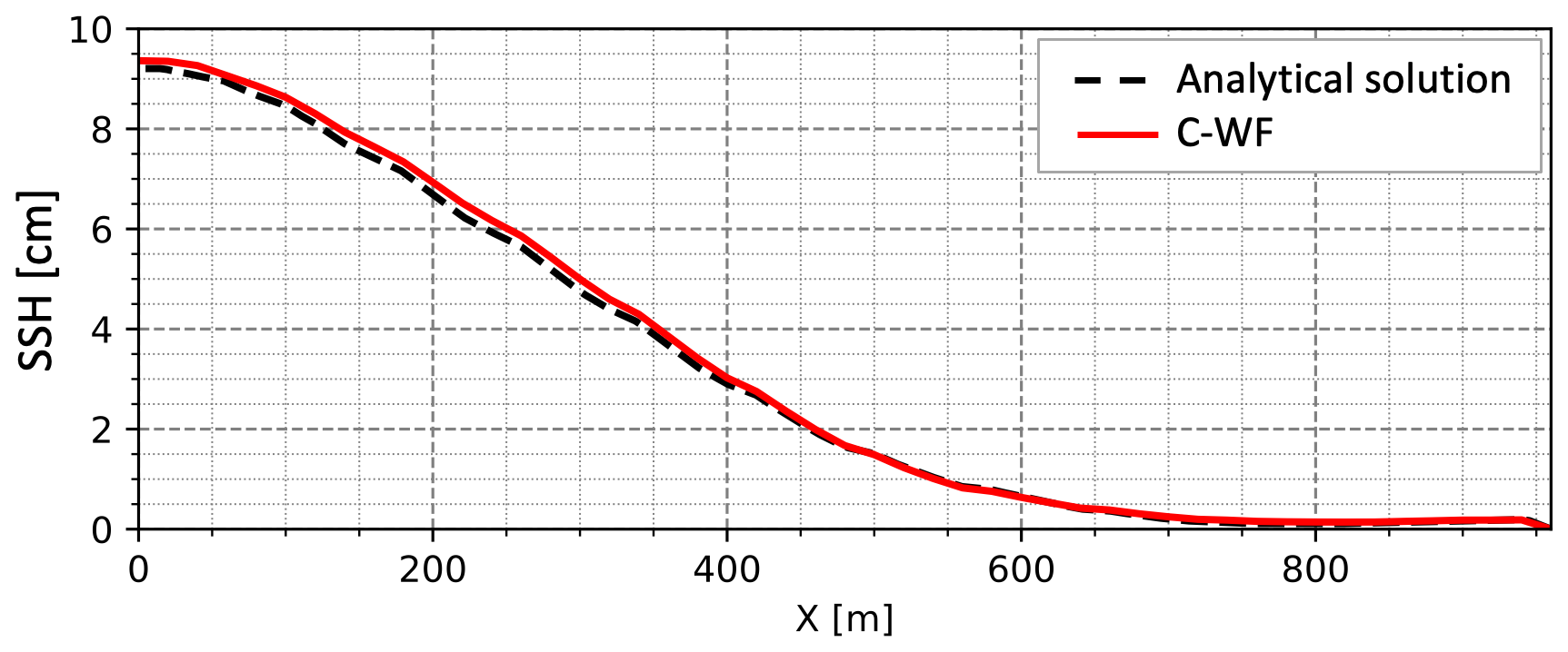
Figure 3 Planar beach test case: comparison between model and analytical solution along the transect 1–2 shown in Fig. 2a. The test case verifies the C-WF simulation, assessing the role of wave setup (via radiation stresses) to the total water level.

The planar beach is a gently sloping square basin with a side length of 960 m, as illustrated in Fig. 2a. The bathymetry is constant along the shore and slopes linearly from 0 to 12 m in the cross-shore direction. The numerical grid has 5400 elements and 2797 nodes and a horizontal resolution of approximately 20 m. The vertical discretization consists of 12 z levels, each with a thickness of 1 m. The wave model is forced along the open boundary by waves with a 2 m significant wave height (SWH), a peak period of 10 s, and a 10° oblique angle relative to the shore-normal direction, using a JONSWAP spectral shape. The circulation model starts from a resting state and is only influenced by the radiation stress from the WW3 model, with no other external forcings applied. These simulation conditions are derived from Xia et al. (2020).

As the waves propagated from the offshore open boundary within the model domain, they start to shoal and break approximately 600 m from the shore, at which point the depth-induced breaking criterion is met. As shown in Fig. 3, the simulated surface elevation produced by the circulation model matches properly with the analytical solution (Wang and Sheng, 2016; Xia et al., 2004).

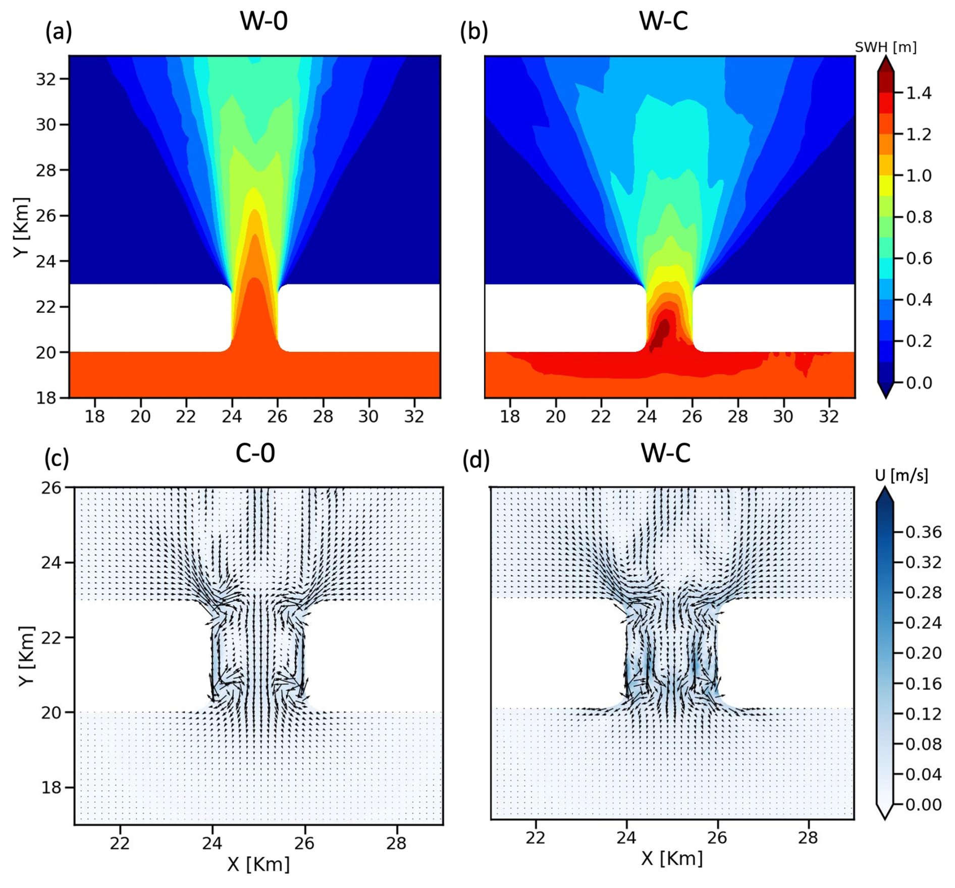
Figure 4 Wave-forced coastal inlet at steady condition: significant wave height for the wave-only simulation (a) and for the two-way wave–current coupled simulation (b); currents for the wave-to-current forced simulation (c) and for the two-way wave–current coupled simulation (d).

3.2 The coastal inlet

A second benchmark defined as coastal inlet is used in this study to conduct a series of simulations that highlight the interactions between waves and sea level. These simulations enable the assessment of wave-induced circulation, the impact of currents on wave dynamics, and the mutual interactions between waves and currents. We conducted several simulations using the following configurations: W-0, an uncoupled wave model simulation; C-0, an uncoupled circulation model simulation; C-WF, where the wave model exclusively supplies fields to the circulation model; and W-C, the two-way coupled configuration. The outcomes of our simulations are then compared with those reported in the existing literature, as cited in the discussion of the results.

The tidal inlet (Fig. 2b) used in this study is derived from the work of Cobb and Blain (2002), based on Kapolnai et al. (1996). The domain recreates an inner basin (lagoon or embayment) measuring 20 km by 10 km, linked to an outer ocean basin of 49 km by 20 km on the continental shelf via a narrow 3 km long and 2 km wide channel. The bathymetry shows a linear slope from a depth of 14 m offshore to 5 m at the channel's entrance, with a consistent depth of 5 m beyond the channel. The unstructured grid resolution is approximately 125 m within the channel and the surrounding area and 1 km throughout the remainder of the domain.

The simulation conditions, as in Cobb and Blain (2002), are detailed as follows. The wave model is forced at the lateral open boundary with a wave field featuring a peak period of 10 s, a SWH of 1 m, and a JONSWAP spectral shape. The waves are set perpendicularly to the southern boundary of the domain. Two different boundary conditions are applied to the offshore boundary depending on the type of simulation. If the circulation model is forced only with waves, a zero-gradient boundary condition is enforced along this boundary to simulate an unperturbed sea surface (in this region wave-induced setup/setdown should not be significant). When the circulation is forced with both waves and tides, the offshore boundary elevation is modulated with specified M2 tidal component with 0.15 m amplitudes and zero phase at the boundary.

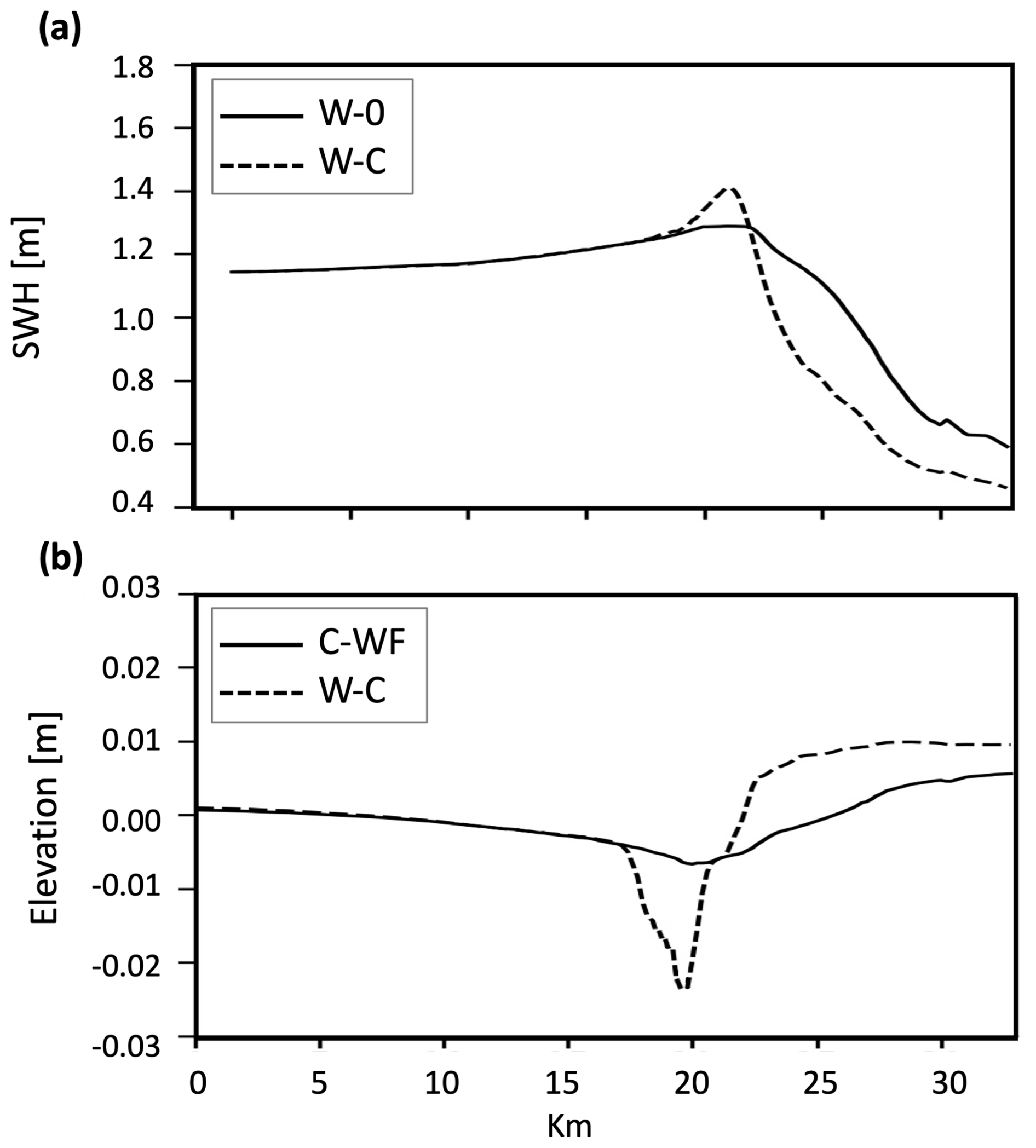
Figure 5 SWH (a) and water elevation (b) of the transects along section 1–2 as indicated in Fig. 2b. The figures replicate the Cobb and Blain (2002) simulations: in (a) we compare W-0 and W-C simulations, while in (b) we compare C-WF with the W-C experiment.

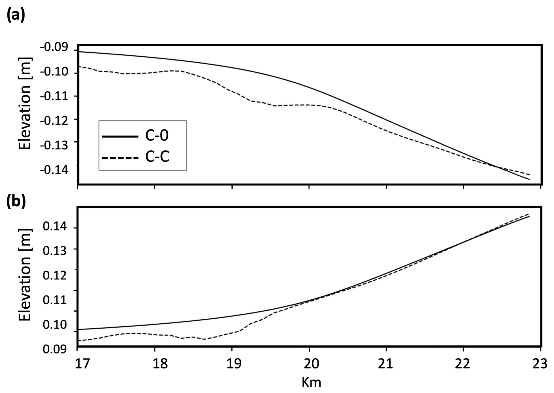
Figure 6 Magnification (at 17–23 km) of the water level along the transect 1–2 shown in Fig. 2b for configuration C-0 and W-C in a tidally driven framework during the ebb (a) and flood (b) phase.

In Fig. 4 we present a snapshot of the results at the 48 h time step from the two uncoupled simulations W-0 (Fig. 4a) and C-0 (Fig. 4c), as well as the coupled W-C (Fig. 4b and d) simulations, with a magnification on the area of the inlet as indicated in Fig. 2. The area of magnification is reduced in the plots showing the currents to better appreciate the vectors' patterns. In the experiment W-0 (Fig. 4a), the wave field demonstrates a homogeneous SWH of approximately 1.2 m as it approaches the inlet, with a reduction along the boundary of the inlet and a spread of around 60° in the lagoon, reaching a maximum SWH of about 0.8 m at the northern boundary. The W-C experiment (Fig. 4b) displays a markedly different and asymmetric pattern, as shown in previous work such as in Cobb and Blain (2002). The maximum SWH in this domain exceeds 1.4 m, and at the mouth of the inlet, the SWH is higher than in the uncoupled experiment. The wave spread in the lagoon is larger, around 80°, and the maximum SWH at the northern boundary is lower than the uncoupled simulation, reaching a maximum of 0.5 m. According to the difference in spreading, we can assume that it is caused by wave refraction induced by non-uniform currents, which enhances both physical and numerical spreading. On the other hand, W-0 exhibits reduced numerical diffusion, which is a characteristic of the WW3 high-order propagation schemes, as the one used here. Interestingly, the presence of currents in W-C appears to mitigate this phenomenon. The simulation C-0 (Fig. 4c) depicts the currents along the inlet, revealing four small meanders at the corners of the inlet and a central jet flanked by two eddies. Additionally, two large, nearly symmetrical eddies are observed in the lagoon. In the coupled simulation W-C (Fig. 4d), the four meanders shift towards the center, resulting in the formation of two eddies between the meanders and the inlet walls. The central jet is less pronounced compared to the C-0 simulation, and the velocities at the inlet mouth, diverging outward, are more intense. This increased intensity contributes to the rise in significant wave height (SWH) observed in Fig. 4b. Inside the lagoon, the pattern of two large eddies is less pronounced, and a significant current is observed.

Following the work of Cobb and Blain (2002), we compared different simulations along the transect 1–2 (shown in Fig. 2b). In the first validation at the 48 h time step, we qualitatively analyze the pattern of SWH from two configurations (Fig. 5a). The W-0 configuration describes the shoaling of waves entering the inlet and lagoon well. The SWH exhibits a gradual increase to a maximum of approximately 1.1 m at 20 km from the southern boundary, followed by a reduction to 0.6 m at 30 km. The pattern observed in the coupled experiment W-C aligns with W-0 up to about 16 km, where the waves begin to be influenced by the currents flowing outward from the lagoon. This interaction causes refraction, resulting in steeper and higher waves that exceed 1.3 m around 18 km. As a result, the waves begin to break earlier and more intensely, leading to a rapid drop of SWH to 0.6 m at 28 km.

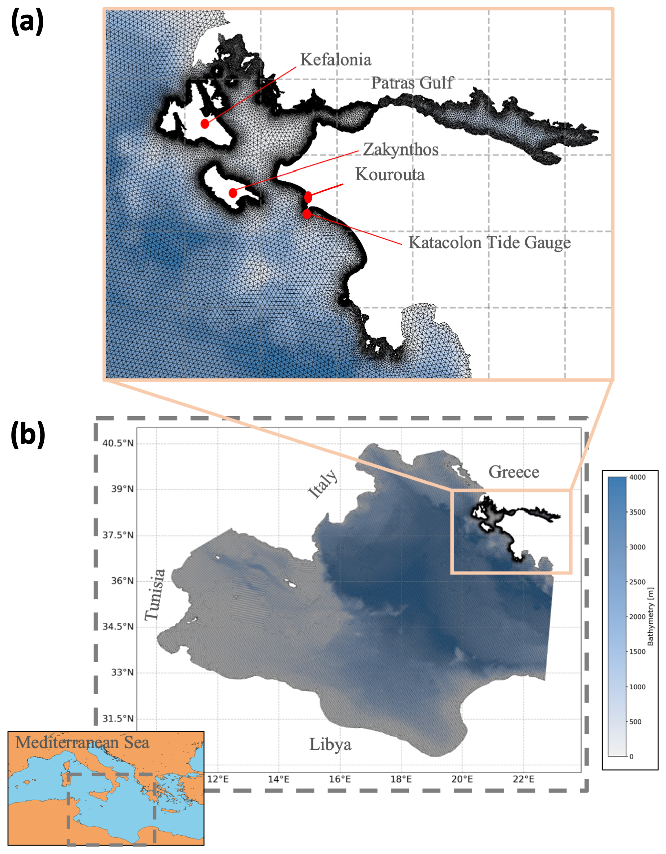
Figure 7 Spatial unstructured grid and bathymetry for the Ionian Sea (b) used for the Medicane Ianos simulation, with an enlarged view on refined areas of affected area (a).

Figure 5b effectively illustrates the coastal processes of wave setup and setdown, as well as the complex interaction between currents and waves near the coast. In this plot, the water level is at rest and theoretically should remain constant at 0 m. The impact of wave forcing, namely the contribution of radiation stress to the circulation, is evident from the deviation of water elevation from the rest condition. A setdown corresponds well with the wave shoaling indicated by W-0 in Fig. 5a, reaching approximately −5 mm at 20 km from the southern boundary and +5 mm with a steeper slope at 33 km in experiment C-WF.

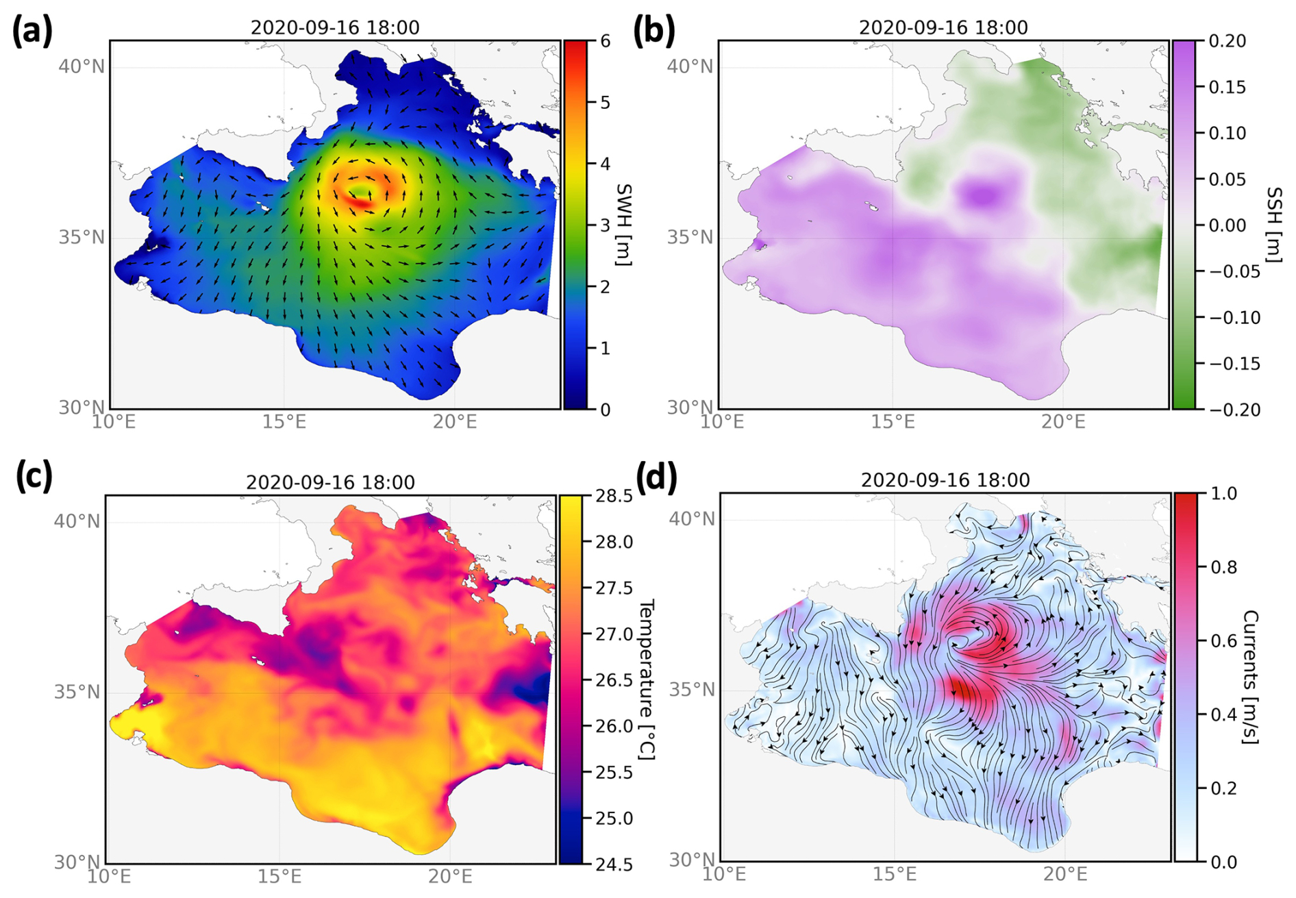
Figure 8 Maps of significant wave height (a), sea level (b), sea surface temperature (c), and surface circulation (d) on 16 September 2020 18:00 UTC (peak time in open ocean) for the entire domain from a two-way coupled simulation.

Table 2 Datasets used in this study.

Wave setup and setdown are further amplified in the fully coupled configuration W-C, where current-induced refraction and breaking result in a higher momentum flux to the water. This configuration exhibits a negative peak of setdown at −2.5 cm and a positive peak of setup at +1 cm, consistently occurring at around 25 km.

The last analysis of wave–current interaction in an idealized test case examines the differences between the C-0 and W-C configurations within a tidally driven framework (Fig. 6). During both flood (Fig. 6a) and ebb (Fig. 6b) phases, the smoother tidal profiles observed in C-0 are perturbed by the wave field interactions in the W-C simulation. The differences between the configurations are slightly larger during the flood phase, around 1.5 cm, and less than 1 cm during the ebb phase of setdown. Both phases indicate a wave setup occurring beyond 22 km.

In all the qualitative validations (Figs. 4–6), the new coupled framework presented in this work produces accurate results that align with the expected physical behavior and are consistent with findings from other studies in the literature (Cobb and Blain, 2002; Wu et al., 2011; Xia et al., 2020). This agreement is evident in both the spatial pattern and the range of variation for sea level and SWH, indicating that the model accurately captures not only the general shape and structure of the observed sea level and wave height patterns but also the magnitude and fluctuations in their values.

4 Simulation of circulation–wave fields during Medicane Ianos

Medicane Ianos was one of the most intense Mediterranean storms since the onset of satellite observation (von Schuckmann et al., 2022). It is notable for its duration and severity, resulting in significant rainfall, flooding, damage, and fatalities (Zekkos et al., 2020). It originated off the Libyan coast near the Gulf of Sidra on 14 September 2020 and moved toward the Ionian Sea and Greece between 17 and 20 September. The storm intensified as it moved northward and eastward, reaching peak strength on 16 September and passing through central Greece, particularly impacting the regions around Karditsa and Farsala. Ianos eventually weakened as it shifted southeast towards Crete. With wind speeds reaching 110 km h⁻¹, the storm caused widespread flooding and destruction, leading to four fatalities in Greece and substantial damage, including the flooding of approximately 5000 properties in Karditsa alone (a slew of weather events – including two named storms troubling Europe – pose challenges far and wide; Yale Climate Connections, 2024).

4.1 Setup of the model

The numerical domain, shown in Fig. 7, encompasses the entire central South Mediterranean Sea, with three open lateral boundaries: in the Otranto Channel to the north, the Strait of Sicily to the west, and the Ionian Sea (between Greece and Libya) to the east. The domain is discretized with an unstructured grid, featuring a horizontal resolution of approximately 2 km offshore, 1 km along the coasts, and 50 m in the area where Medicane Ianos made landfall in Greece, including the islands of Zakynthos and Kefalonia.

The circulations and wave models are forced with atmospheric fields from ECMWF analysis data (10 km resolution and 6 h frequency). The surface fields are corrected along the coastal boundaries following the sea-over-land procedure described in Kara et al. (2008). The atmospheric variables used for the circulation include 2 m air temperature, 2 m dew point temperature, total cloud cover, mean sea level atmospheric pressure, and total precipitation. Meridional and zonal 10 m wind components are used for both wave and circulation models.

The modeling approach is based on the downscaling of Copernicus Marine Service¹ products released at the Mediterranean Sea regional scale. The circulation model is three-dimensionally nested into the MEDSEA_MULTIYEAR_PHY product (Table 2) both in terms of initialization and open boundaries. The scalar fields (sea level, temperature, and salinity) are treated through a clamped boundary condition, while the velocity fields are imposed as a nudged boundary condition using a relaxation time of 3600 s.

The wave model is initialized using a parametric fetch-limited spectrum based on the initial wind field and is forced at the lateral open boundaries by the MEDSEA_MULTIYEAR_WAV product (Table 2). Mean wave parameters, such as significant wave height, mean wave direction, and peak period, are used to reconstruct the wave spectra, following the approximation described by Yamaguchi (1984).

The model outputs are saved at 1 h frequency.

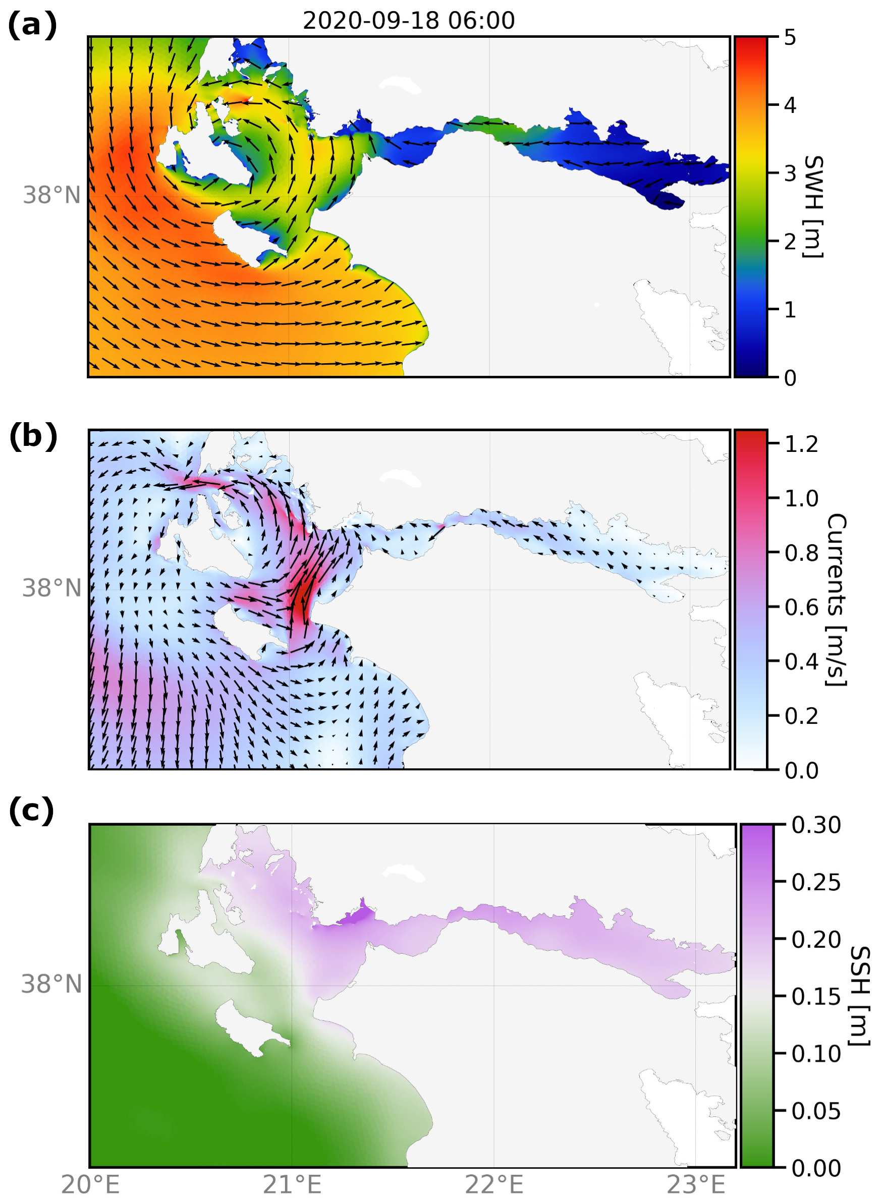
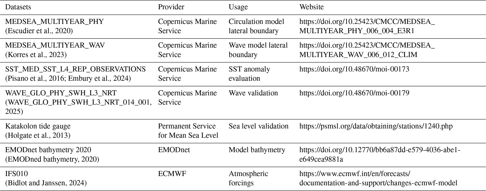
Figure 9 Maps of significant wave height (a), surface circulation (b), and sea level (c) on 18 September 2020 at 06:00 UTC (peak time in coastal zones of Greece) for the Greek coastal areas from the two-way coupled simulation (W-C).

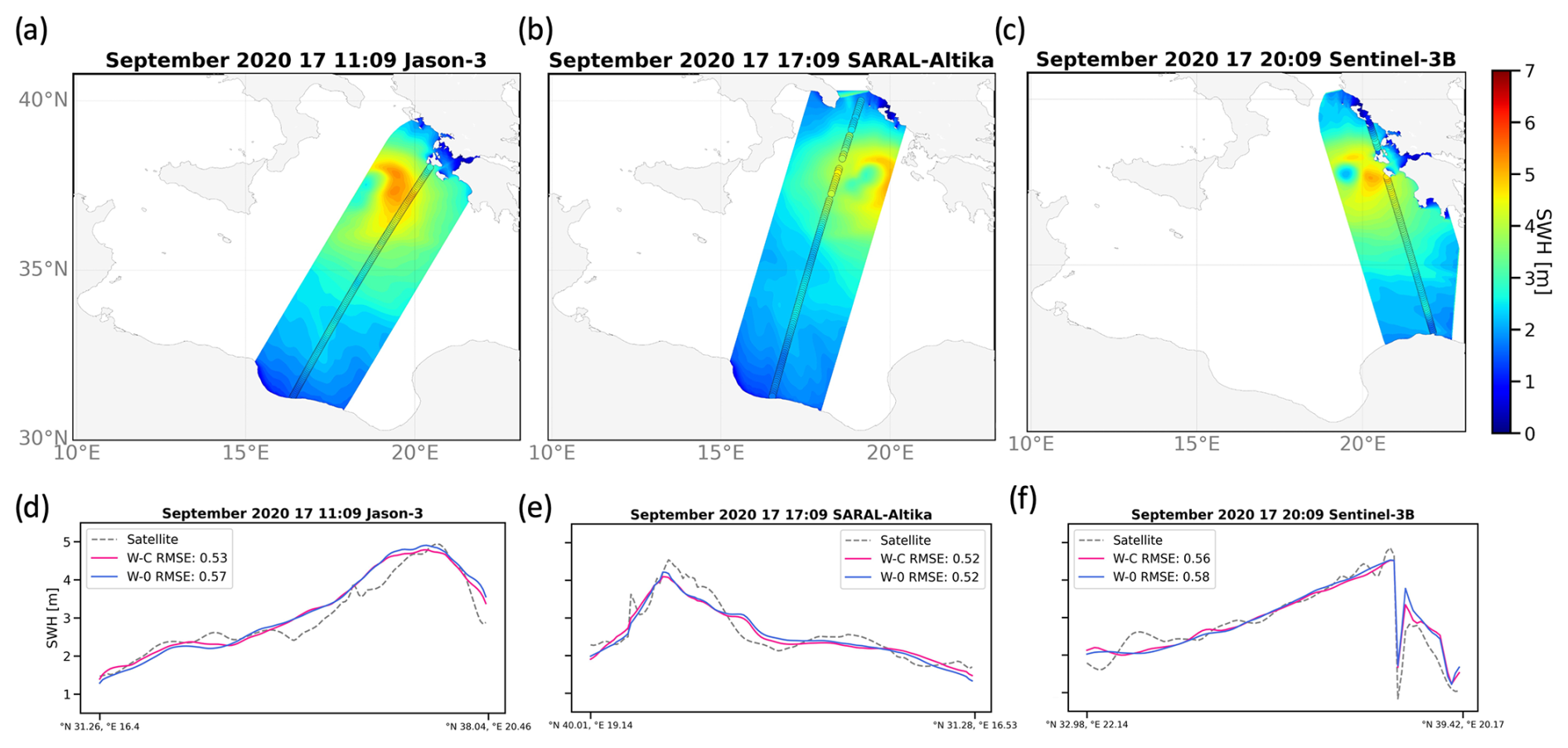
Figure 10 Maps of SWH against satellite altimeter (Jason3, SARAL-AltiKa, Sentinel-3b) tracks (inset circles) for the W-C configuration (a–c). SWH along-track comparison between the two model configurations and satellite tracks is reported in (d)–(f).

4.2 Results and discussion

Medicane Ianos reached its maximum intensity at 18:00 UTC on 16 September 2020, as it entered the Ionian Sea (Fig. 8). The coupled modeling framework provides a comprehensive analysis of the event, revealing the storm's extensive impact on the wave field across the central Mediterranean Sea. The affected area spans over 5° × 5°, with significant wave heights averaging over 3 m and reaching up to 6 m in the eyewall region (Fig. 8a). The influence of Medicane Ianos on sea level is clear, as a pronounced positive sea level anomaly exceeding +20 cm is observed, particularly within the storm's core (Fig. 8b). This anomaly stands out against the low-tide conditions, providing a distinct footprint of the storm. Although sea surface temperature does not exhibit a consistent pattern at the storm's peak, cooler waters are noticeable in the southeastern region of Sicily (Fig. 8c). Additionally, the sea surface currents display a well-defined pattern, with velocities exceeding 1 m s⁻¹ along the eyewall and a divergent flow branching northeastward and southeastward (Fig. 8d).

At 06:00 on 18 November, Medicane Ianos made landfall in Greece, impacting the islands of Zakynthos and Kefalonia, as well as the Gulf of Patras (Fig. 9). The SWH simulated during this event, as shown in Fig. 9a, is notably high for this region of the Mediterranean, reaching up to 4.5 m along the western coastlines of the islands. The cyclonic circulation associated with Medicane Ianos intensifies the waves on the northern part of the Gulf of Patras, which is particularly affected due to the nearly perpendicular wave direction. Furthermore, the confluence of currents from the north and south of Zakynthos (Fig. 9b) results in current speeds reaching up to 1.2 m s⁻¹ in this convergence zone. The combined impact of these high waves and strong currents leads to a significant storm surge, exceeding 30 cm, in the northern part of the Gulf of Patras (Fig. 9c).

In the following sections, we investigate the effect of the coupling on the simulation of Medicane Ianos.

4.2.1 Effects of circulation on waves

The validation of the wave model results and the difference between the W-C and W-0 configurations are shown in this paragraph using two approaches. In Fig. 10 we compare the simulations with the satellite altimeter tracks (WAVE_GLO_PHY_SWH_L3_NRT; Table 2) which crossed Medicane Ianos. In details, three altimetric measurements from Jason-3, SARAL-AltiKa, and Sentinel-3B are available on 17 September, and the SWH results from the W-C configuration are overlapped with the satellite measurement and shown in Fig. 10a–c, respectively. The model simulates the extreme event with a very high quality, and the patterns of the modeled wave field match with good agreement the satellite data. For Jason-3 and Sentinel-3B the measured SWH reaches 5 m, while for SARAL-AltiKa, the SWH is slightly lower because the track is slightly eastward of Medicane Ianos. Figure 10d–f illustrate the along-track validation for both the W-C and W-0 configurations. This analysis is based on the nearest point between the observation and the model in both space and time dimensions. The difference between the two configurations can be a few tens of centimeters in some cases, while in others the time series overlap. However, the W-C configuration demonstrates a reduction of approximately 3 %–4 % for the root mean square error (RMSE) for Jason-3 (Fig. 10d) and Sentinel-3B (Fig. 10f) tracks. It is worth mentioning that, although this analysis shows better peak predictions for the W-0 configuration, the W-C  configuration more closely matches the observations overall, both during growth and decay phases. A potential motivation for the reduction of SWH at peaks in the coupled experiment is due to the alignment of currents and wind, which reduces wind stress. This is attributed to the fact that the absolute wind speed used to force the wave model is modified into relative wind by the presence of currents.

For a more robust assessment of the wave model, we analyze the time window including the days Medicane Ianos persisted over the central Mediterranean Sea, from 15 to 19 September (Fig. 11). From this investigation, the model exhibits a very high accuracy in representing the extreme event, with a correlation coefficient of 0.95, a negative bias of approximately 20 cm, and a RMSE of 33 cm. The comparison of W-C to W-0 shows a reduction in bias of around 6 % and a decrease in error of approximately 3 % in the coupled configuration, confirming the previous findings of Causio et al. (2021). In this study, we do not present through attribution simulations the explicit quantification of contribution of the air-stability parameter and currents. This decision is based on our prior investigations, which have already demonstrated their effectiveness and role (Causio et al., 2021; Clementi et al., 2017).

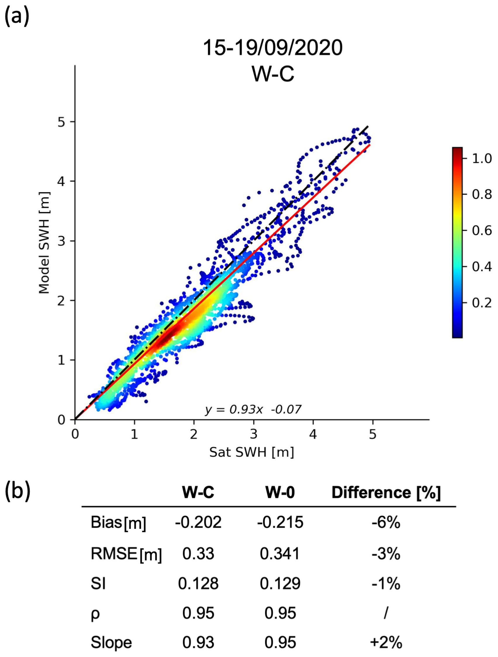
Figure 11 (a) SWH scatterplot for the W-C configuration is shown, with colors indicating the plot density of occurrence. The black line represents the best-fit line, while the red line denotes the linear regression of the data. (b) Statistics (root mean square error – RMSE, bias, scatter index – SI, Pearson's correlation coefficient – ρ, and the slope of the fit) are summarized and expressed in meters, providing comparisons for the W-C and W-0 configurations as well as the percentage difference between them.

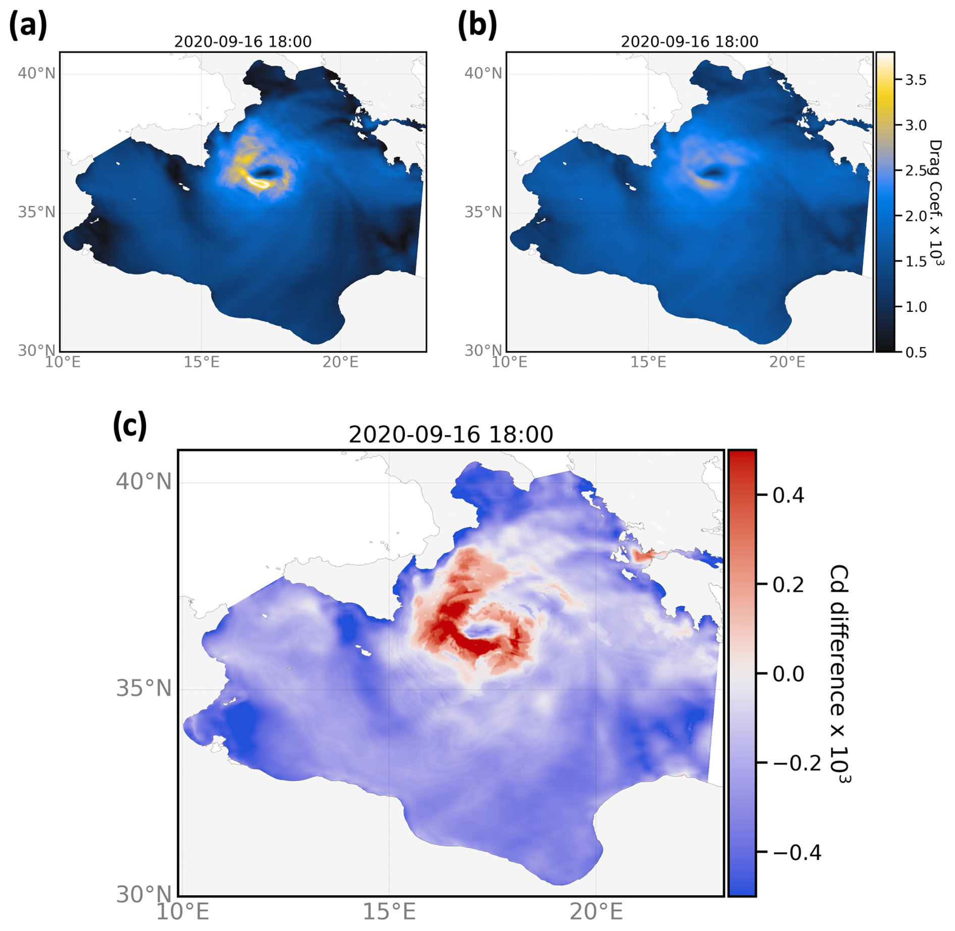
Figure 12 Maps of drag coefficient (C_d) at the peak event in open ocean (16 September 2020 at 18:00). (a) Drag coefficient computed by WW3 in the W-C experiment. (b) Drag coefficient computed via Hellerman and Rosenstein (1983) in the C-O experiment. (c Difference between (a) and (b).

4.2.2 Effects of waves on circulation

In Fig. 12 we illustrate the drag coefficient (C_d) from the W-C (Fig. 12a) and C-0 (Fig. 12b) configurations at the peak of the event (16 September 2020 at 18:00) and their differences (Fig. 12c). The C_d from the uncoupled simulation, which is derived from the Hellerman and Rosenstein (1983) formulation, exhibits a more homogeneous field and overall higher values with respect to the coupled system, except in the area of the Ianos passage at the peak time, where the coupled simulation is able to provide larger C_d values. Significant differences between the sea-state-dependent drag (W-0) and the Hellerman and Rosenstein (1983) formulation (used in C-0) occur in regions farther from Medicane Ianos (see Fig. 8a), particularly in the northern Ionian Sea, the eastern part of the study domain, and the Gulf of Gabes. Additionally, the wider range for C_d allows higher values to be reached; the C-0 configuration never exceeds the value of 2.5 × 10⁻³, while the W-C configuration goes beyond 3.5 × 10⁻³. In both configurations, the pattern of extreme drag is asymmetric, with the southern part of Medicane Ianos experiencing the highest values.

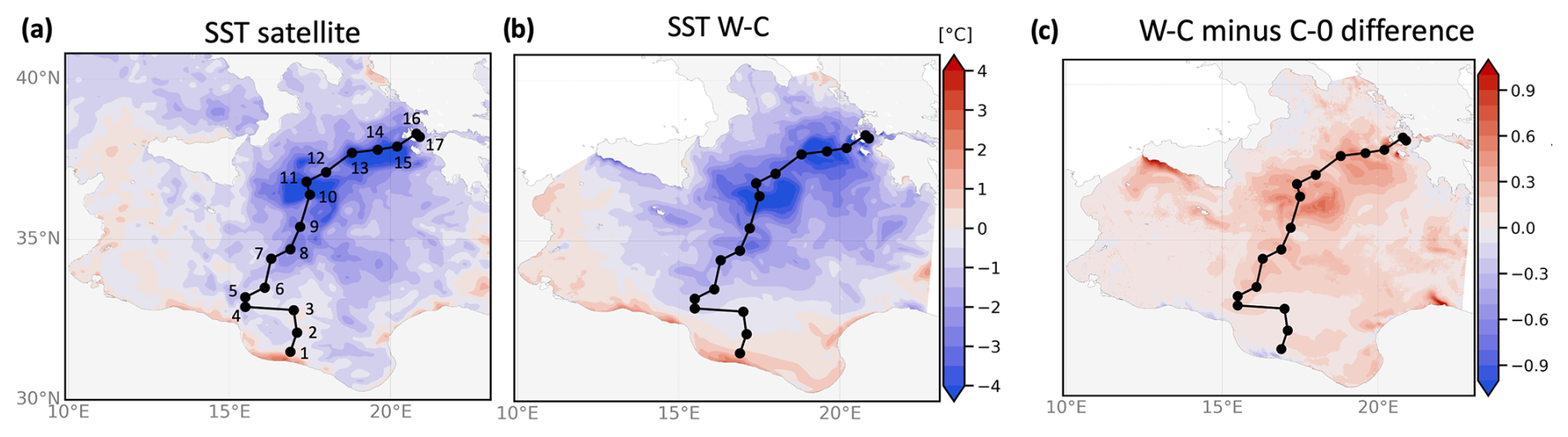
Figure 13 Sea surface temperature anomaly (°C) between 19 September (after Ianos) and 14 September (before Ianos) from satellite (a), two-way coupled model W-C (b), and SST difference between the anomaly of W-C and C-0 (c). The black path represents the Medicane Ianos path identified as the minimum sea level pressure location every 6 h. In panels (a) and (b) the color bar range is set to [−4, 4 °C] to better highlight the footprint pattern, even though the difference reached −5 °C.

The passage of a strong cyclone over a water body induces surface cooling due to both upwelling and increased evaporation (Price, 1981). In Fig. 13, we present the sea surface temperature (SST) footprint induced by Ianos' passage over the central Mediterranean Sea, following the approach of Clementi et al. (2022). The footprint results from the comparison of the SST of the day after Medicane Ianos hit Greece (19  September) with the SST of the day before Ianos' formation (14 September). The footprint is computed for L4 gridded satellite observations (Table 2) (Fig. 13a), W-C configuration (Fig. 13b), and C-0 configuration (not shown). Additionally, the difference between the footprints of W-C and C-0 is shown in Fig. 13c. Specifically, for the satellite data, the foundation temperature is used, which approximately corresponds to the sea temperature during the nighttime at a depth of around 2–5 m. For this reason, in this analysis we used the model temperature at midnight at a depth of 3 m.

The SST footprint from the satellite shows a general cooling of the central Mediterranean Sea, with the exception of the southern coasts, and two distinct areas of larger significant cooling. The southern Ionian Sea, where Medicane Ianos experiences its highest intensity, shows the largest cooling, dropping the temperature down by −5 °C. Here the footprint follows the Medicane Ianos track with a northeast orientation.

A qualitative comparison between the satellite data and the W-C and C-0 configurations illustrates that both configurations exhibit adequate patterns but show a stronger impact on SST compared to the observations. However, the W-C configuration demonstrates slightly warmer behavior (Fig. 13c), and the footprint's width is narrower than in C-0, more closely matching the pattern observed in satellite data. These differences can be attributed to the sea-state-dependent drag coefficient, which modifies the circulation in the area.

Furthermore, Fig. 13 shows the path of Medicane Ianos as it passed through the Ionian Sea (from Libya at point 1 to Greece at point 17), highlighting the location of the sea level pressure minimum every 6 h.

Consequently, we analyze the vertical profile of model temperature along the Medicane Ianos track (Fig. 14) for both the W-C and C-0 configurations. In this assessment we compute, as in Fig. 13, the temperature anomaly between 19 and 14 September and then the difference between W-C and C-0. The range of temperature anomaly spans from approximately −0.6 to 0.6 °C. Notably, the largest difference between the two configurations occurs in the Ionian Sea, particularly from point 10 onward. Throughout the track, the W-C configuration is warmer in the mixed layer, with the latter generally being slightly shallower in the coupled simulation, with a few exceptions at points 3 and 14, where the uncoupled configuration exhibits a slightly thinner mixed layer. As Medicane Ianos moves towards Greece, the plot indicates that the W-C configuration footprint is even warmer in the mixed layer than C-0, and even colder below the pycnocline, suggesting a strengthening of the stratification in W-C. Points 13 and 14 are peculiar because they show warmer W-C even below the mixed layer up to 60 m. This difference can be attributed to the less intense upwelling observed in the W-C configuration, which results in smaller cold wedges (located at points 10–12 and 13–15 in Fig. 13) compared to those in the C-0 configuration.

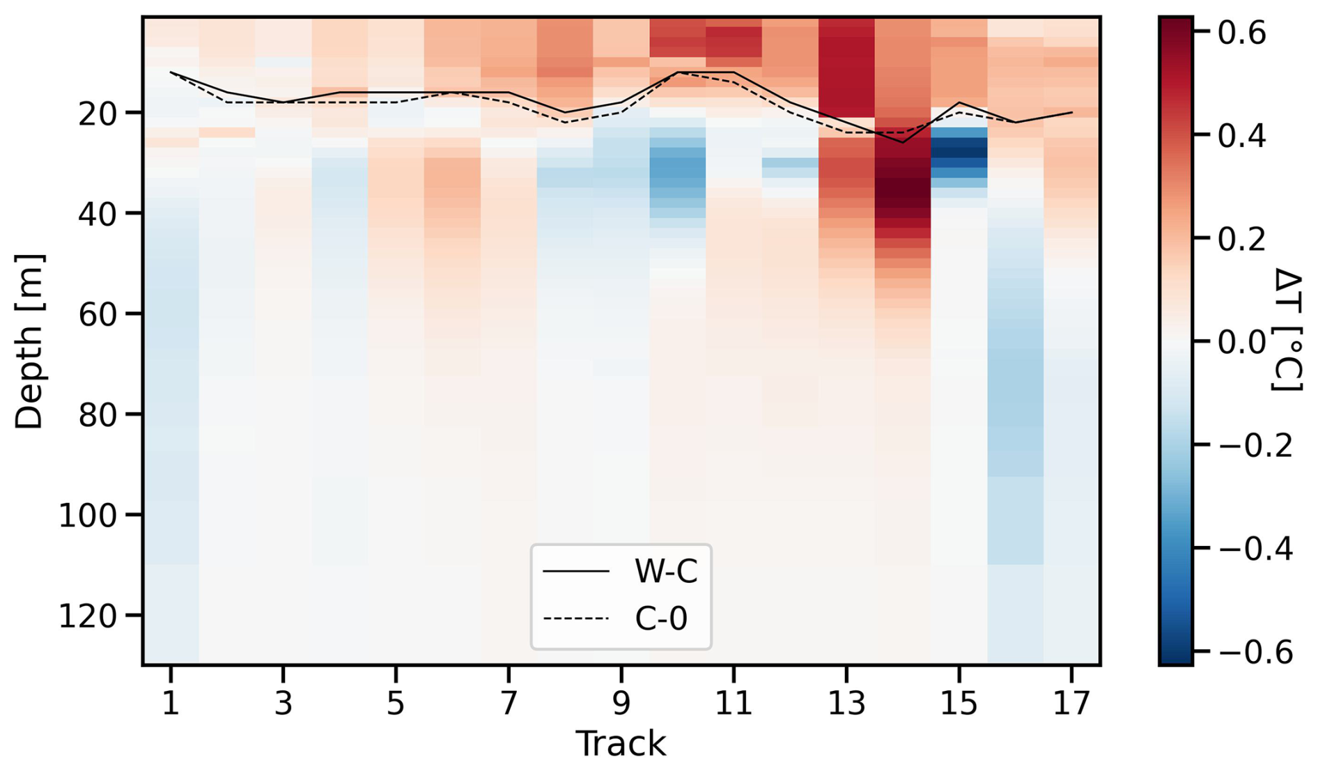
Figure 14 Anomaly temperature difference between W-C and C-0 for the Medicane Ianos passage over the central Mediterranean Sea. Black lines refer to the mixed layer depth for W-C (solid line) and C-0 (dashed line). The x axis corresponds to the locations shown in Fig. 3a.

This suggests that the impact of this coupling on the vertical structure is primarily confined to the uppermost 50 m in the central Mediterranean Sea. Nevertheless in some cases, such as in coastal areas, the impact extends deeper, reaching up 100 m and beyond.

One of the main contributions expected from this coupled modeling framework is the enhanced capability to predict storm surges, by inclusion of the radiation stresses. Sensitivity tests with C_d + radiation stress and radiation stress only showed differences below 1 %, while the C_d-only case closely matched the W-0 simulation (results not shown).

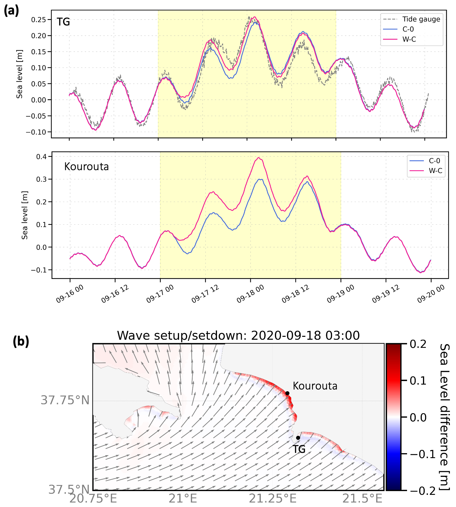
Figure 15 Time series of TWL for C-0 and W-C configurations. In plot (a), upper panel, the models are compared with observed data at Katakolon tide gauge – TG (in dashed gray). In the plot (b), bottom panel, the model configurations are compared at the Kourouta beach. The shaded yellow area highlights the two days impacted by the Medicane Ianos-induced surge. Plot (b) highlights the wave setup (in red) and setdown (in blue), computed as the TWL difference between C-0 and W-C. Additionally, it shows the location of the time series (in plot a), as well as the mean wave direction represented by vectors.

Medicane Ianos was chosen for this study because it made landfall close to the Katakolon tide gauge, which provides a suitable reference for comparison between the sea level observations and the W-C and C-O configurations (Fig. 15). The C-0 configuration demonstrates good accuracy in predicting sea level at the tide gauge location; however, the W-C configuration represents more accurately the storm surge induced by Medicane Ianos (the event is highlighted in yellow in Fig. 15a). Both configurations show nearly identical performance under normal conditions (before and after the event). The maximum difference between the two configurations is 4 cm, allowing the W-C configuration to simulate more precisely the two peaks of the storm surge. Notably, the inclusion of wave effects led to a more rapid drop in surge after the storm passage, improving also the fit for the first tide trough after the storm (the third tide trough within the yellow area in Fig. 15a). It is worth mentioning that the wave contribution to the Ianos storm surge is approximately 10 % at the peak of the event, although this value can be significantly higher in other situations. To illustrate this, Fig. 15a, bottom panel, shows the same time series comparison for a location a few kilometers away from the tide gauge, along the nearby beach of Kourouta. The plot reveals that the waves provide a larger contribution in this location, resulting in a surge about 11 cm higher than the one shown in C-0, accounting for roughly 30 % of the total contribution. The difference between the time series, as shown in Fig. 15c, can be attributed to the wave field direction, which makes the tide gauge partially sheltered, while the beach faces more orthogonal waves. The significance of wave direction is further emphasized along the northern shoreline, where the wave setup is even more intense due to the waves being nearly orthogonal to the coast. Notably, the wave contribution to the storm surge during Medicane Ianos is comparable in percentage to findings of Dietrich et al. (2011) for hurricanes Katrina and Rita in the Gulf of Mexico and Kim et al. (2010) during Typhoon Anita in the South China Sea.

5 Conclusions

This study represents the first two-way coupling of the SHYFEM-MPI model with WW3 using an external coupler, marking an advancement in the simulation of storm surges during extreme events like Medicane Ianos. Our primary goal is the evaluation of storm surge dynamics. Nevertheless, together with radiation stress, we also incorporated additional coupled physical processes, such as sea-state-dependent wind stress, Doppler shift, sea-level-dependent water depth for wave physics, and the inclusion of effective wind based on air stability parameters. Rigorous validation through well-established idealized test cases, including the tidal inlet and planar beach scenarios, confirms the reliability of our coupled modeling framework.

The real-case simulation and comparison of coupled versus uncoupled configurations highlight the added value of incorporating the wave component in storm surge simulations, particularly for coastal applications. Notably, during Medicane Ianos, wave setup contributes to approximately 10 % of the sea level variation at the Katakolon tide gauge, with a significantly greater impact – around 30 % – in nearshore areas. The inclusion of a sea-state-dependent drag coefficient introduces larger dynamics to the simulations, with a lower drag in areas distant from the storm and increased drag near the eyewall of Medicane Ianos.

Our findings indicate that the coupling effects are more pronounced in the northern part of Medicane Ianos' path, where the storm intensity is largest. The coupling leads to a slightly thinner and warmer mixed layer and, in some locations, affects the water column up to 100 m, likely due to reduced upwelling of deeper waters. The impact of circulation on wave dynamics is appreciable, as coupling reduces bias by approximately 6 % and overall error by around 3 % in the wave model.

The numerical framework developed in this study proves to be an effective tool for simulating both large-scale and coastal processes, with a particular strength in describing storm surge dynamics. This system holds significant potential for enhancing coastal hazard identification, early warning systems, and the management and planning of sea and coastal activities. The encouraging results from this work lay the foundation for further development, including the integration of additional processes such as Stokes drift, sea-state-dependent vertical mixing, and bottom stress (their importance has been shown in several studies such as Breivik et al., 2015; Alari et al., 2016; Staneva et al., 2017; Couvelard et al., 2020), which are currently neglected or parameterized in this version of the circulation model.

Appendix A

This implementation primarily aimed to improve the coupling mechanism between SHYFEM-MPI and WW3, enhancing their capability in modeling extreme events. However, for the sake of completeness in describing this methodology and coupled system, we provide additional details on the coupling procedure performance.

The coupled system is more computationally demanding than the individual models, with the computational time of the coupled system approximately 30 % longer than that of the standalone wave model. We emphasize the wave model because it represents the primary bottleneck between the two models. While this increase in computational time was not a major concern in our study or in operational use, refactoring the system to improve performance could be beneficial for long hindcast applications.

Regarding CPU coherency, we conducted twin simulations using 144 and 216 cores and compared the results. The average difference for all the output variables over the 7 d simulation is shown in Table A1.

Figure A1 illustrates the time evolution of the difference in selected variables (not all, to maintain clarity) between the two simulations. The discrepancies stabilize around 10⁻⁶–10⁻⁵ after 2 d of simulation. For this type of application, these results are satisfactory, especially considering that SHYFEM-MPI was not compiled with the bit-wise reproducibility option and that the error remains within the limits of single-precision floating-point operations.

Table A1 Summary of the average differences in the investigated variables after a 7 d simulation using 144 and 216 cores.

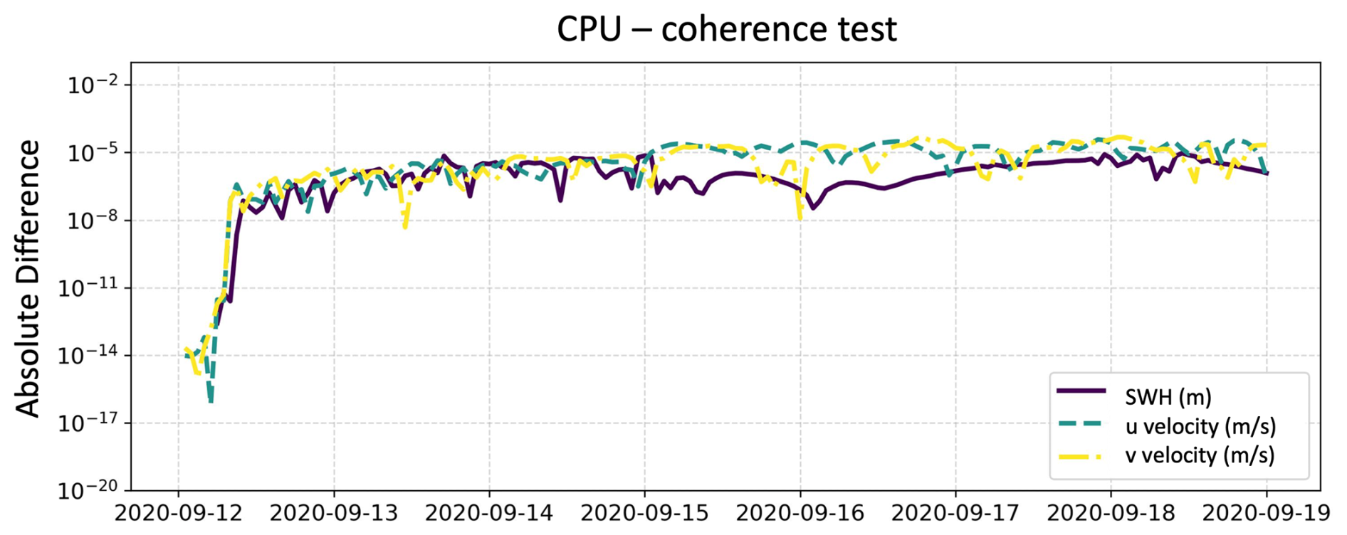
Figure A1 Error evolution over a 7 d simulation for u–v and SWH variables using 144 and 216 cores.