Sensitivity study of energy transfer between mesoscale eddies and wind-induced near-inertial oscillations

Analyses of current observations and numerical simulations at two moorings in the northern South China Sea reveal the transfer of near-inertial energy between the background currents associated with mesoscale eddies and near-inertial currents (NICs). A series of numerical experiments are conducted to determine important parameters affecting the energy transfer between idealized mesoscale eddies and NICs generated by rotating winds. Speeds of NICs transferred by both cyclonic and anticyclonic mesoscale eddies increase linearly with the wind stress and eddy strength. The transferred NICs in anticyclonic eddies have current amplitudes about 6 times larger than in cyclonic eddies. The translation speed of the mesoscale eddy and the wind rotation frequency also affect the conversion of NICs. The energy transfer rate is elevated with the increase in the positive Okubo–Weiss parameter. A simple theoretical analysis is conducted to verify our findings based on numerical results. Analytical solutions confirm the evident asymmetry of the energy transfer between anticyclonic and cyclonic eddies and quantitatively demonstrate the relationship between the wind stress and the near-inertial energy transferred by mesoscale eddies.

1 Introduction

Near-inertial oscillations (NIOs) are very common in the global ocean and they appear as a prominent peak in the spectrum of ocean currents (Garrett, 2001). NIOs contain almost half the total kinetic energy of the internal waves and significantly contribute to the vertical shear in the internal waveband (Ferrari and Wunsch, 2009). When surface winds with high spatiotemporal variations act at the ocean surface, strong NIOs could occur in the ocean surface mixed layer (SML; Chen et al., 2015a; D'Asaro et al., 1995; Pollard and Millard, 1970). At the base of the SML, near-inertial internal waves (NIWs) are generated through the horizontal convergence and divergence of the SML (Gill, 1984). These NIWs are free to radiate to the thermocline and deep waters, and low-mode NIWs with long wavelengths can propagate at least hundreds of kilometers toward the Equator from their source regions (Alford, 2003; Jochum et al., 2013; Munk and Wunsch, 1998). NIOs not only affect the energy, momentum, and material transport in the upper ocean, but also play an important role in maintaining diapycnal mixing and global ocean circulation (Chen et al., 2016; Greatbatch, 1984; Jing et al., 2016; Price et al., 1986; Wunsch and Ferrari, 2004).

Due to the turbulent and inhomogeneous nature of the ocean, the central frequency of NIOs is influenced by the β effect and shows a significant blue or red shift induced by the relative vorticity of mesoscale eddies (Chen et al., 2015b; Elipot et al., 2010; Kunze, 1985; Mooers, 1975; Perkins, 1976; Sun et al., 2011). If the magnitude of the gradient in the relative vorticity is larger than the β effect (Chelton et al., 2011), mesoscale eddies also modulate the energy distribution and propagation of the near-inertial motions (van Meurs, 1998; Wang et al., 2024). Previous studies of current observations in the northwestern South China Sea (nSCS) demonstrated that the near-inertial energy propagates both upwards and downwards under the influence of the anticyclonic eddies (Chen et al., 2017; Zhai et al., 2007). Using in situ observations and ray-tracing techniques, Jaimes and Shay (2010) demonstrated that anticyclonic eddies trap the near-inertial kinetic energy, which rapidly propagates vertically below the thermocline and even to the deep ocean. Young and Jelloul (1997) suggested that anticyclonic eddies can improve the vertical propagation rate of the near-inertial energy by deepening the thermocline. Zhai et al. (2005) demonstrated that wind-generated near-inertial kinetic energy is also high in strong mesoscale motion regions. Based on a numerical study, Lelong et al. (2020) reveled that anticyclonic eddies facilitate the energy transfer from wind-driven inertial energy to propagating waves. Fer et al. (2018) found that sub-inertial waves trapped within the Lofoten Basin eddy can significantly contribute to the observed turbulence in the eddy.

Mesoscale eddies and NIOs are energetic in the SML (Bühler and McIntyre, 2005; Vanneste, 2013; Xie and Vanneste, 2015). Mesoscale eddies not only change the spatial distribution of NIOs, but also exchange energy with NIOs through nonlinear interaction (Muller, 1976; Thomas, 2012). Based on observational studies of specific NIO events, Noh and Nam (2020) found that mesoscale eddies can effectively enhance the intensity of NIOs. Energy transfer also occurs between NIOs and low-frequency geostrophic currents through nonlinear interaction (Liu et al., 2023; Thomas, 2012; Whalen et al., 2020). Jing et al. (2018) demonstrated that the large-scale geostrophic currents of the Gulf Stream affect the distribution of near-inertial energy. Whitt and Thomas (2015) suggested that, in a unidirectional laterally sheared geostrophic flow, a continuous energy transfer occurs between mesoscale eddies and NIOs. In the Kuroshio extension, due to the change in the effective Coriolis frequency caused by the relative vorticity of mesoscale eddies, the energy exchange efficiency between the anticyclonic eddies and NIOs is about twice that between the cyclonic eddies and NIOs (Jing et al., 2017). Based on numerical results in the Icelandic Basin, Barkan et al. (2021) found that a significant energy transfer occurs between NIOs and sub-inertial motions, with the energy transfer rate in winter and summer about half and a quarter of the local near-inertial wind energy input, respectively. The above and other studies suggested that the energy transfer processes between mesoscale eddies and NIOs should play an important role in the ocean energy cascade (Alford et al., 2016; Ford et al., 2000; McWilliams, 2016; Thomas, 2017). Nevertheless, most previous studies focused on the energy transfer rate and efficiency. There is a knowledge gap in the amplitude of the near-inertial energy transferred by the mesoscale eddy and the sensitivity of the abovementioned energy transfer to mesoscale eddies and wind parameters. The main objective of this study is to quantity the energy transfer between mesoscale eddies and wind-induced NIOs.

This paper is structured as follows. Section 2 provides a brief description of observational data and reanalysis used in this study. Section 3 presents the original and modified slab models. Model results for the energy transfer between mesoscale eddies and the NIOs are given in Sect. 4. A series of sensitivity experiments for determining the important factors affecting the energy transfer is presented in Sect. 5. The results of sensitivity experiments are verified through theoretical analysis in Sect. 6. A summary and discussion are given in Sect. 7.

2 Observational and reanalysis data

Current observations at two subsurface moorings named S2 and S3 in the nSCS (marked in Fig. 1) are analyzed here (Chen, 2023). The current observations at these two moorings were made using acoustic Doppler current profilers (ADCPs). Mooring S2 is located at 117°39.619^′ E and 21°37.001^′ N, with a water depth of 499 m. Current observations at this location were made at depth bins from 58 to 442 m from 22 August 2016 to 8 May 2017. At ADCP mooring S2, the vertical sampling interval is 16 m and the time internal is 60 min. ADCP mooring S3 is located at 117°26.528^′ E and 21°52.945^′ N, with a water depth of 266 m. Current observations at this mooring were made at depth bins from 37 to 229 m during the same observational period as at location S2. At mooring S3, the vertical sampling interval is 8 m and the time internal is 30 min.

Hourly winds at 10 m above the mean sea level in the nSCS were extracted from the European Centre for Medium-Range Weather Forecasts (ECMWF) ERA5 reanalysis. The ERA5 winds from July 2016 to June 2017 with an interval of 1 h and a horizontal resolution of 0.25° are used to calculate the hourly wind stress to be used as the model forcing (Hersbach et al., 2023). The wind speed data obtained from ERA5 are widely used in previous research on near-inertial motions in the northwestern Pacific.

The surface geostrophic currents used in this study were derived from the sea level grid data provided by the Copernicus Atmosphere Monitoring Service (C3S). The sea surface height anomaly and geostrophic current data in the nSCS from July 2016 to June 2017 are used here, which have a horizontal resolution of 0.25° and a time interval of 24 h (C3S, 2018).

The mixed layer depth (MLD) for the nSCS was extracted from the 2018 edition of the World Ocean Atlas (WOA2018) (http://www.ncei.noaa.gov/products/world-ocean-atlas, last access: 1 September 2022), with a horizontal resolution of 0.25° (Boyer et al., 2019). The MLD at each location is defined as the depth at which the vertical change in the potential density from the ocean surface is 0.125 (sigma units).

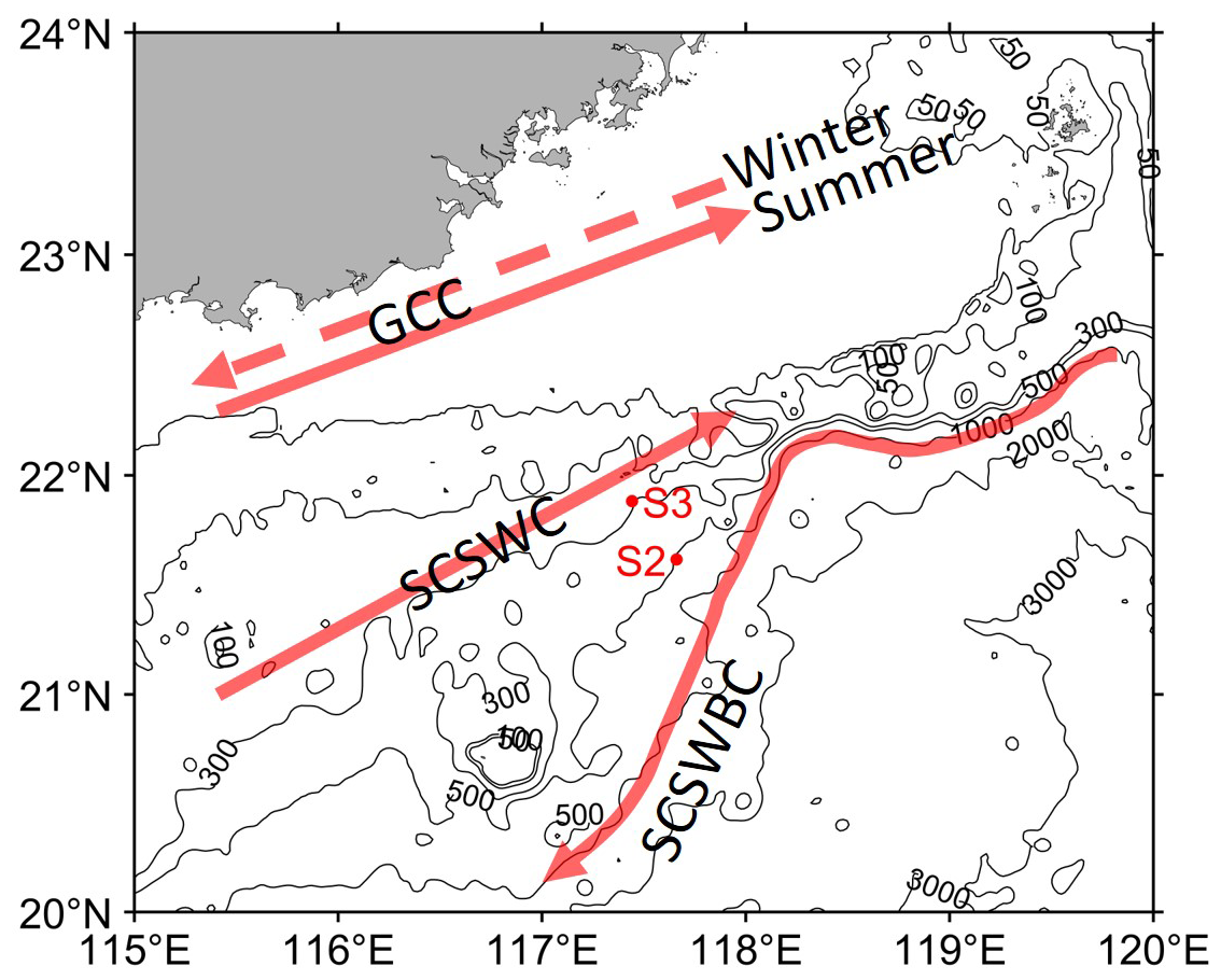
Figure 1 Major bathymetric features and circulation (from Shu et al., 2018) of the northern South China Sea. The two red dots represent the locations of two ADCP moorings named S2 and S3. Black contours represent isobaths in meters. GCC refers to the Guangdong Coastal Current, SCSWC refers to the South China Sea Warm Current, and SCSWBC refers to the South China Sea western boundary current. The solid (dashed) line in the GCC indicates the current direction in summer (winter).

3 Method

3.1 Strain and vorticity of a mesoscale field

The vertical component of the relative vorticity (ζ) has been used to measure the rate of fluid rotation within a mesoscale eddy, which is defined as

$$\begin{array}{}\text{(1)}& \mathit{\zeta }={\displaystyle \frac{\partial V}{\partial x}}-{\displaystyle \frac{\partial U}{\partial y}},\end{array}$$

where U and V are zonal (eastward) and meridional (northward) surface geostrophic currents, respectively.

The effective Coriolis frequency (f_eff) is defined as (Kunze, 1985)

$$\begin{array}{}\text{(2)}& f_{\mathrm{eff}}=f+{\displaystyle \frac{\mathit{\zeta }}{\mathrm{2}}},\end{array}$$

where f is the inertial frequency.

The normal and shear components of the rate of strain tensor, S_n and S_s, are defined as

$$\begin{array}{}\text{(3)}& {\displaystyle }{S}_{\mathrm{n}}={\displaystyle \frac{\partial U}{\partial x}}-{\displaystyle \frac{\partial V}{\partial y}},\text{(4)}& {\displaystyle }{S}_{\mathrm{s}}={\displaystyle \frac{\partial V}{\partial x}}+{\displaystyle \frac{\partial U}{\partial y}}.\end{array}$$

The relative importance of total strain and relative vorticity is diagnosed with the Okubo–Weiss parameter (Okubo, 1970):

$$\begin{array}{}\text{(5)}& \mathrm{OW}=S_{\mathrm{n}}^{\mathrm{2}}+S_{\mathrm{s}}^{\mathrm{2}}-{\mathit{\zeta }}^{\mathrm{2}}.\end{array}$$

In this study, the dependence of the energy transfer between the mesoscale eddy and NICs on the relative vorticity is considered.

3.2 Modified slab model

A simple linear model known as the slab model (Pollard and Millard, 1970) was used in simulating NIOs in the SML. Analysis of observed currents in the nSCS (to be discussed in Sect. 4) demonstrates that NIOs can also occur in the SML under nearly steady winds. This suggests the importance of the energy transfer between the background currents and near-inertial currents (NICs). To investigate this energy transfer, the background geostrophic currents (U and V) are added to the original slab model as the modified slab model (Jing et al., 2017; Weller, 1982):

$$\begin{array}{}\text{(6)}& \left\{\begin{array}{l}\frac{\partial u}{\partial t}+u\frac{\partial U}{\partial x}+v\frac{\partial U}{\partial y}=fv-ru+\frac{{\mathit{\tau }}_x}{{\mathit{\rho }}_o{H}_{\mathrm{mix}}}\\ \frac{\partial v}{\partial t}+u\frac{\partial V}{\partial x}+v\frac{\partial V}{\partial y}=-fu-rv+\frac{{\mathit{\tau }}_y}{{\mathit{\rho }}_o{H}_{\mathrm{mix}}}\end{array}\right.,\end{array}$$

where u and v are zonal and meridional currents averaged vertically in the SML, and H_mix is the MLD. The damping coefficient r is set to $\mathrm{1}/\mathrm{8}$ d⁻¹, which is used to parameterize the loss of near-inertial energy. In Eq. (6), f is the inertial frequency, and ρ_o is the seawater density set to be 1024 kg m⁻³. Wind stress components (τ_x, τ_y) are calculated using ERA5's 10 m winds with the drag coefficient suggested by Oey et al. (2006).

The above modified slab model uses two important assumptions: the Rossby number of the geostrophic currents is assumed to be far less than 1 and the horizontal scale of winds to be much larger than that of mesoscale eddies. By ignoring the background geostrophic currents, the above modified slab model becomes the original slab model, which was used in many previous studies examining the inertial response in the SML (D'Asaro, 1985; Paduan et al., 1989; Pollard and Millard 1970).

The modified slab model in Eq. (6) can be solved numerically using an implicit numerical scheme in time to obtain NICs in the SML:

$$\begin{array}{}\text{(7)}& \left\{\begin{array}{l}\frac{u^{n+\mathrm{1}}-u^n}{\mathrm{\Delta }t}+u^{n+\mathrm{1}}{U}_x^{n+\mathrm{1}}+v^{n+\mathrm{1}}{U}_y^{n+\mathrm{1}}\\ =f{v}^{n+\mathrm{1}}-r{u}^{n+\mathrm{1}}+\frac{{\mathit{\tau }}_x^{n+\mathrm{1}}}{\mathit{\rho }{H}_{\mathrm{mix}}}\\ \frac{v^{n+\mathrm{1}}-v^n}{\mathrm{\Delta }t}+u^{n+\mathrm{1}}{V}_x^{n+\mathrm{1}}+v^{n+\mathrm{1}}{V}_y^{n+\mathrm{1}}\\ =-f{u}^{n+\mathrm{1}}-r{v}^{n+\mathrm{1}}+\frac{{\mathit{\tau }}_y^{n+\mathrm{1}}}{\mathit{\rho }{H}_{\mathrm{mix}}}\end{array}\right.,\end{array}$$

where Δt is the time step, which is set to 3600 s in this study, and subscripts x and y in U and V represent partial derivatives. The initial value of the NICs is set to 0. In Eq. (7), variables with superscripts n and n+1 represent their values at time nΔt and (n+1)Δt, respectively.

After merging some terms, the numerical scheme of the modified slab model can be written as

$$\begin{array}{}\text{(8)}& \left\{\begin{array}{l}\frac{u^{n+\mathrm{1}}-u^n}{\mathrm{\Delta }t}+a_{\mathrm{1}}^{n+\mathrm{1}}{u}^{n+\mathrm{1}}+b_{\mathrm{1}}^{n+\mathrm{1}}{v}^{n+\mathrm{1}}=c_{\mathrm{1}}^{n+\mathrm{1}}\\ \frac{v^{n+\mathrm{1}}-v^n}{\mathrm{\Delta }t}+a_{\mathrm{2}}^{n+\mathrm{1}}{u}^{n+\mathrm{1}}+b_{\mathrm{2}}^{n+\mathrm{1}}{v}^{n+\mathrm{1}}=c_{\mathrm{2}}^{n+\mathrm{1}}\end{array}\right.,\end{array}$$

where $a_{\mathrm{1}}=U_x+r$, $a_{\mathrm{2}}=V_x+f$, $b_{\mathrm{1}}=U_y-f$, $b_{\mathrm{2}}=V_y+r$, $c_{\mathrm{1}}={\mathit{\tau }}_x/\mathit{\rho }{H}_{\mathrm{mix}}$, and $c_{\mathrm{2}}={\mathit{\tau }}_y/\mathit{\rho }{H}_{\mathrm{mix}}$.

Equation (8) can be written in the following tensor form:

$$\begin{array}{}\text{(9)}& \begin{array}{rl}& \left[\begin{array}{cc}{a}_{\mathrm{1}}^{n+\mathrm{1}}+\frac{\mathrm{1}}{\mathrm{\Delta }t}& b_{\mathrm{1}}^{n+\mathrm{1}}\\ a_{\mathrm{2}}^{n+\mathrm{1}}& b_{\mathrm{2}}^{n+\mathrm{1}}+\frac{\mathrm{1}}{\mathrm{\Delta }t}\end{array}\right]\left\{\begin{array}{c}{u}^{n+\mathrm{1}}\\ v^{n+\mathrm{1}}\end{array}\right\}\\ & =\left\{\begin{array}{c}\frac{u^n}{\mathrm{\Delta }t}+c_{\mathrm{1}}^{n+\mathrm{1}}\\ \frac{v^n}{\mathrm{\Delta }t}+c_{\mathrm{2}}^{n+\mathrm{1}}\end{array}\right\}.\end{array}\end{array}$$

The numerical update equations for currents are given as

$$\begin{array}{}\text{(10)}& {\displaystyle }\begin{array}{rl}{u}^{n+\mathrm{1}}& ={\displaystyle \frac{\mathrm{1}+\mathrm{\Delta }t{b}_{\mathrm{2}}^{n+\mathrm{1}}}{\left(\mathrm{1}+\mathrm{\Delta }t{a}_{\mathrm{1}}^{n+\mathrm{1}}\right)\left(\mathrm{1}+\mathrm{\Delta }t{b}_{\mathrm{2}}^{n+\mathrm{1}}\right)-\mathrm{\Delta }t{b}_{\mathrm{1}}^{n+\mathrm{1}}{a}_{\mathrm{2}}^{n+\mathrm{1}}}}\\ & \left[{\displaystyle \frac{u^n}{\mathrm{\Delta }t}}+c_{\mathrm{1}}^{n+\mathrm{1}}-{\displaystyle \frac{\mathrm{\Delta }t{b}_{\mathrm{1}}^{n+\mathrm{1}}}{\mathrm{1}+\mathrm{\Delta }t{b}_{\mathrm{2}}^{n+\mathrm{1}}}}\left({\displaystyle \frac{v^n}{\mathrm{\Delta }t}}+c_{\mathrm{2}}^{n+\mathrm{1}}\right)\right],\end{array}\text{(11)}& {\displaystyle }\begin{array}{rl}{v}^{n+\mathrm{1}}& ={\displaystyle \frac{\mathrm{1}+\mathrm{\Delta }t{a}_{\mathrm{1}}^{n+\mathrm{1}}}{\left(\mathrm{1}+\mathrm{\Delta }t{a}_{\mathrm{1}}^{n+\mathrm{1}}\right)\left(\mathrm{1}+\mathrm{\Delta }t{b}_{\mathrm{2}}^{n+\mathrm{1}}\right)-\mathrm{\Delta }t{b}_{\mathrm{1}}^{n+\mathrm{1}}{a}_{\mathrm{2}}^{n+\mathrm{1}}}}\\ & \left[{\displaystyle \frac{u^n}{\mathrm{\Delta }t}}+c_{\mathrm{1}}^{n+\mathrm{1}}-{\displaystyle \frac{\mathrm{\Delta }t{a}_{\mathrm{2}}^{n+\mathrm{1}}}{\mathrm{1}+\mathrm{\Delta }t{a}_{\mathrm{1}}^{n+\mathrm{1}}}}\left({\displaystyle \frac{v^n}{\mathrm{\Delta }t}}+c_{\mathrm{2}}^{n+\mathrm{1}}\right)\right].\end{array}\end{array}$$

3.3 Analysis of NICs

The observed zonal and meridional currents at 58.3 m below the sea surface at location S2 and at 37.7 m at location S3 (marked in Fig. 1) in the nSCS are analyzed to estimate the near-inertial kinetic energy in the SML. The observed NICs are obtained by using a bandpass filter through Fourier transform with a frequency band of 0.85f–1.15f.

The surface geostrophic currents described in Sect. 2 are specified in the modified slab model based on the assumption that the geostrophic currents are vertically uniform in the SML during the study period. The simulated currents by the original and modified slab models are band-passed through Fourier transform with the frequency band of 0.85f–1.15f and are further smoothed using a running window of two inertial periods to obtain the simulated amplitude of NICs.

To quantitatively assess performances of the original and modified slab models, correlation analysis and root mean square error (RMSE) analysis between the original slab model, the modified slab model, and observations are respectively made.

4 Results

4.1 Observed NICs

Time series of observed NICs at the top depth bins (58.3 m at S2 and 37.7 m at S3) of two subsurface ADCP moorings (known as ${\mathit{u}}_{\mathrm{S}\mathrm{2}}^{\mathrm{top}}$ and ${\mathit{u}}_{\mathrm{S}\mathrm{3}}^{\mathrm{top}}$) are shown in black lines in Fig. 2 during the observational period from day 234 (22 August 2016) to day 492 (7 May 2017) with respect to 1 January 2016. Intense NICs were generated and lasted for about 11 d from day 293 to day 304 under the largest wind forcing (∼ 1.6 N m⁻²) on day 293 (Fig. 2e and f). The largest speed of NICs was ∼ 0.30 m s⁻¹ on day 295 at the top depth bin at mooring S2 (Fig. 2a) and ∼ 0.37 m s⁻¹ on day 296 at the top depth bin at mooring S3 (Fig. 2b). Some NICs were also excited on other days when the winds were relatively weak and nearly steady.

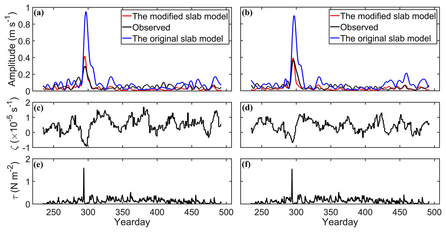
Figure 2 Speeds (m s⁻¹) of observed (black line) and simulated NICs at the top depth bins of ADCP observations at moorings (a) S2 and (b) S3. Red and blue lines denote model results produced by the modified slab and original slab models, respectively. Time series of relative vorticity of the surface geostrophic currents at moorings (c) S2 and (d) S3 and time series of wind stress at moorings (e) S2 and (f) S3. The “year day” is defined as the number of days elapsed since 00:00:00 (GMT) on 1 January 2016.

Observed NICs at other depth bins of these two ADCP moorings reveal that intense NICs occurred on days 293–304 at depths between 60 and 200 m at mooring S2 (not shown) and these NICs originated from the SML. At mooring S3, similar intense NICs occurred at depths between 40 and 180 m on days 280–305 (not shown), and these NICs also originated from the SML. On days 306–318, in comparison, moderate NICs occurred in the lower layer between 150 and 310 m at these two moorings.

It should be noted that the current observations (${\mathit{u}}_{\mathrm{S}\mathrm{2}}^{\mathrm{top}}$ and ${\mathit{u}}_{\mathrm{S}\mathrm{3}}^{\mathrm{top}}$) at the top bins of the two ADCP moorings are in the lower part of the SML or below the SML during the observational period. Based on WOA2018, the climatological monthly mean MLD at the two ADCP moorings is the thinnest and ∼ 20 m in August (days 234–243) and increases to the maximum value of ∼ 90 m in January (days 366–396). The MLD decreases from ∼ 56 m in February (days 397–424) to ∼ 37 m in May (days 486–492) and is about 25 m in June and July. This suggests that the observed NICs at the top depth bin (58.3 m) of S2 were made in the lower part of the SML in December and January (days 335–396) but below the SML on the other days of the observational period (Fig. 2a). By comparison, the observed NICs at the top depth bin (37.7 m) of S3 were made in the middle of the SML in December and January (days 335–396) and in the lower part of the SML in October and November (days 274–334) and February–May (days 397–492).

The relative vorticity estimated from the surface geostrophic currents was negative at the two moorings on days 290–300 (Fig. 2c and d), with maximum negative values of about −0.92 × 10⁻⁵ s⁻¹ (−0.17f) at mooring S2 and about −0.68 × 10⁻⁵ s⁻¹ (−0.13f) at mooring S3. The negative values of the relative vorticity during this period resulted from the westward propagation of an anticyclonic eddy. As shown in Fig. 3a and f, moorings S2 and S3 were located over the area between a relatively strong anticyclonic eddy and a weak cyclonic eddy on day 295. The anticyclonic eddy moved westward and passed mooring S2 before day 316 (Fig. 3b and g). On day 316, the relative vorticity was low and positive of about 1.23 × 10⁻⁵ s⁻¹ (0.23f) at mooring S2 and 0.83 × 10⁻⁵ s⁻¹ (0.15f) at mooring S3.

On days 350–450, an anticyclonic eddy moved southwestward and passed through moorings S2 and S3 (Fig. 3c, d, h, and i). There was a weak cyclonic eddy close to the two moorings on day 435 (Fig. 3d and i). The relative vorticity was relatively strong and positive during this period, with maximum positive values at about 1.68 × 10⁻⁵ s⁻¹ (0.31f) on day 380 at mooring S2 and 1.29 × 10⁻⁵ s⁻¹ (0.24f) on day 423 at mooring S3.

Between days 451–492, there is a weak anticyclonic eddy close to moorings S2 and S3, and the two moorings are located at the edge of the anticyclonic eddy on day 452 (Fig. 3e and j).

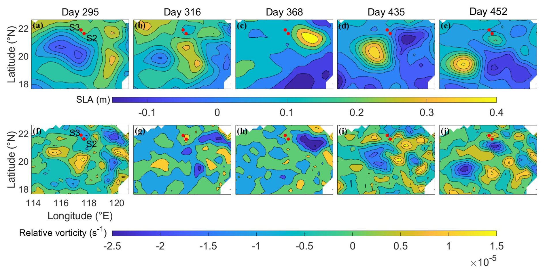
Figure 3 Spatial distributions of sea surface level anomaly (SLA) on day 295 (a), day 316 (b), day 368 (c), day 435 (d), and day 452 (e). Spatial distributions of the relative vorticity on day 295 (f), day 316 (g), day 368 (h), day 435 (i), and day 452 (j). The two red dots mark the locations of two ADCP moorings S2 and S3.

4.2 Simulated NICs

Numerical simulations are made using the original and modified slab models to examine whether energy exchange occurs between the mesoscale eddy and NICs in the SML at moorings S2 and S3. Both the original and modified slab models assume that the NICs in the SML are vertically uniform and use the damping coefficient r set to a relatively small value of $\mathrm{1}/\mathrm{8}$ d⁻¹. Both the models are forced by the time series of wind stress shown in Fig. 2e and f.

The simulated NICs produced by the original slab model at the top bins of two ADCP moorings are shown by the blue lines in Fig. 2a and b. The simulated NICs by the original slab model are large and about 0.95 m s⁻¹ (0.90 m s⁻¹) at mooring S2 (S3) on day 296 and relatively weak on days 350–430. In comparison with the observed NICs, the original slab model has a large deficiency of significantly overpredicting the observed large NICs on days 285–300 at the two stations and also moderately overpredicting the observed NICs on other days of the observational period. It should be noted that the results of both the original and modified slab models using three different damping coefficients ($r=\mathrm{1}/\mathrm{5}$, $\mathrm{1}/\mathrm{6}$, and $\mathrm{1}/\mathrm{7}$ d⁻¹) and annual mean MLD at two stations (∼ 45 m) are highly similar with the model results using $r=\mathrm{1}/\mathrm{8}$ d⁻¹ and monthly mean MLD shown in Fig. 2a and b.

In comparison with the original slab model results, the modified slab model generates much smaller NICs than the original slab model on days 280–305 (red lines in Fig. 2a and b), with a maximum value of about 0.42 m s⁻¹ at mooring S2 and about 0.39 m s⁻¹ at mooring S3 on day 295. In comparison with the observed NICs at the two moorings, the modified slab model performs significantly better than the original slab model on days 250–325 and days 451–492, indicating the importance of the energy exchange between the background mesoscale eddies and NICs. On days 350–450, the relative vorticity of the background currents is positive, which results in the simulated NICs produced by the modified slab model being slightly weaker than the observed NICs at these two moorings. As mentioned in Sect. 4.1, the top depth bins of the ADCP observations at the two moorings were in the lower part of the SML or below the SML during the observational period, which partially explains the differences between observed and simulated NICs by the modified slab model shown in Fig. 2a and b. Differences between the observed and simulated NICs can also partially be explained by the assumption of vertically uniform geostrophic currents in the SML and exclusion of baroclinic dynamics.

The above analysis based on results shown in Fig. 2 suggests that, overall, the simulated NICs produced by the modified slab model agree with the observed NICs significantly better than the original slab model at moorings S2 and S3. This indicates the occurrence of near-inertial energy transfer induced by the interaction between mesoscale eddies and NICs in the SML during the observational period.

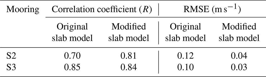
To quantify the model performance, we use the correlation coefficient (R) and the root mean square error (RMSE) based on the time series of observed and simulated NICs shown in Fig. 2a and b. The modified slab model has a higher correlation coefficient ($R=\sim$ 0.81) and smaller root mean square error (RMSE = ∼ 0.04 m s⁻¹) than the original slab model ($R=\sim$ 0.70 and RMSE = ∼ 0.12 m s⁻¹) at mooring S2. At mooring S3, the R value between the observed NICs and results of the modified slab model is ∼ 0.84, and RMSE is ∼ 0.03 m s⁻¹. For the original slab model at location S3, the R value is ∼ 0.85, and RMSE is ∼ 0.10 m s⁻¹. These statistical indices suggest that the modified slab model performs better than the original slab model, especially in reproducing the amplitude of the observed NICs. This also suggests that the energy transfer between mesoscale eddies and NICs may be a non-negligible process in the energy cascade across different scales in the global ocean.

Table 1 Correlation coefficients (R) and RMSEs between the simulation results of the modified and original slab models and observations for the observational period.

5 Sensitivity study

A series of numerical experiments (in total 226) are conducted using the original and modified slab models to examine sensitivity of model results to the wind speed, the wind rotation frequency, the translational speed of the mesoscale eddy, and the strength of the mesoscale eddy. Both the cyclonic and anticyclonic eddies with an idealized eddy structure are used for simplicity. Results of the original and modified slab models are both bandpass-filtered (0.60f–1.40f) to get broad NICs signals and then smoothed using a running window of two inertial periods to obtain the near-inertial velocity in the SML.

5.1 Idealized mesoscale eddy structure

Based on a composite analysis of satellite altimetry and Argo float data, Zhang et al. (2013) suggested a universal structure of mesoscale eddies in the global ocean. Their universal structure of mesoscale eddies is used in our experiments.

The normalized structure $\stackrel{\mathrm{̃}}{P}\left(\stackrel{\mathrm{̃}}{r},z\right)$ of the pressure anomaly in the universal mesoscale eddy used in this study is decomposed into a radial function $R\left(\stackrel{\mathrm{̃}}{r}\right)$ and a vertical function H(z):

$$\begin{array}{}\text{(12)}& {\displaystyle }\stackrel{\mathrm{̃}}{P}\left(\stackrel{\mathrm{̃}}{r},z\right)=R\left(\stackrel{\mathrm{̃}}{r}\right)H\left(z\right),\text{(13)}& {\displaystyle }R\left(\stackrel{\mathrm{̃}}{r}\right)=\left(\mathrm{1}-{\displaystyle \frac{{\stackrel{\mathrm{̃}}{r}}^{\mathrm{2}}}{\mathrm{2}}}\right)e^{-\frac{{\stackrel{\mathrm{̃}}{r}}^{\mathrm{2}}}{\mathrm{2}}},\text{(14)}& {\displaystyle }H\left(z_s\right)=H_{\mathrm{0}}\sin \left(k{z}_s+{\mathit{\theta }}_{\mathrm{0}}\right)+H_{\mathrm{ave}},\text{(15)}& {\displaystyle }\stackrel{\mathrm{̃}}{r}={\displaystyle \frac{r}{R_{\mathrm{0}}}},\text{(16)}& {\displaystyle }{z}_s=\underset{\mathrm{0}}{\overset{z}{\int }}\left({\displaystyle \frac{N}{f}}\right)\mathrm{d}z,\end{array}$$

where r is the radial distance to the eddy center, R₀ is the radius of the mesoscale eddy, N is the buoyancy frequency, H₀, k, θ₀, and H_ave are undetermined coefficients, e.g., in this study, $H_{\mathrm{0}}=\mathrm{2}/\mathrm{3}$, $H_{\mathrm{ave}}=\mathrm{2}/\mathrm{3}$, $N={\mathrm{10}}^{-\mathrm{3}}(\mathrm{1}/s)$, $k=\mathit{\pi }/\mathrm{18}\mathrm{000}$, $f=\mathrm{5}\times {\mathrm{10}}^{-\mathrm{5}}$ rad s⁻¹, and ${\mathit{\theta }}_{\mathrm{0}}=\mathit{\pi }/\mathrm{6}$. The vertical structure function H(z) defined above is similar to the structural diagram in Zhang et al. (2013).

The structure function for the idealized mesoscale eddy in the Cartesian coordinate system can be written as

$$\begin{array}{}\text{(17)}& \begin{array}{rl}\stackrel{\mathrm{̃}}{P}\left(x,y,z\right)& =\left(\mathrm{1}-{\displaystyle \frac{x^{\mathrm{2}}+y^{\mathrm{2}}}{\mathrm{2}{R}_{\mathrm{0}}^{\mathrm{2}}}}\right)\cdot e^{-\frac{x^{\mathrm{2}}+y^{\mathrm{2}}}{\mathrm{2}{R}_{\mathrm{0}}^{\mathrm{2}}}}\\ & \cdot \left[{\displaystyle \frac{\mathrm{2}}{\mathrm{3}}}\cdot \sin \left({\displaystyle \frac{\mathit{\pi }}{\mathrm{900}}}\cdot z+{\displaystyle \frac{\mathit{\pi }}{\mathrm{6}}}\right)+{\displaystyle \frac{\mathrm{2}}{\mathrm{3}}}\right],\end{array}\end{array}$$

with the origin of the coordinate being the eddy center at the sea surface.

Using the pressure anomaly suggested by Wei et al. (2017), the equation for the pressure field based on the different strength of mesoscale eddies can be given as

$$\begin{array}{}\text{(18)}& {\displaystyle }P\left(x,y,z\right)=P_{\mathrm{0}}\cdot \stackrel{\mathrm{̃}}{P}\left(x,y,z\right)+\stackrel{\mathrm{‾}}{P}\left(z\right),\text{(19)}& {\displaystyle }{P}_{\mathrm{0}}=g\cdot {\mathit{\rho }}_{\mathrm{0}}\cdot {\mathrm{SLA}}_{\mathrm{c}},\end{array}$$

where P₀ is the strength of mesoscale eddies, ρ₀ is the reference density of seawater taken as 1024 kg m⁻³, g is the gravitational acceleration set to be 9.8 m s⁻², SLA_c is the sea surface level anomaly (SLA) of the eddy center where the anticyclone eddies are specified as negative values and the cyclonic eddies are positive values, and the average pressure field is denoted by $\stackrel{\mathrm{‾}}{P}$. As only mesoscale eddy signals are added to the ocean in this study, $\stackrel{\mathrm{‾}}{P}$ is a function of the vertical direction that is homogeneous in the horizontal direction.

Using the geostrophic balance, the zonal and meridional components of the geostrophic velocity at the ocean surface are given as

$$\begin{array}{}\text{(20)}& {\displaystyle }u=-{\displaystyle \frac{\mathrm{1}}{{\mathit{\rho }}_{\mathrm{0}}f}}{\displaystyle \frac{\partial P}{\partial y}}=-{\displaystyle \frac{P_{\mathrm{0}}}{{\mathit{\rho }}_{\mathrm{0}}f}}\left[{\displaystyle \frac{y^{\mathrm{3}}+y{x}^{\mathrm{2}}-\mathrm{4}y{R}_{\mathrm{0}}^{\mathrm{2}}}{\mathrm{2}{R}_{\mathrm{0}}^{\mathrm{4}}}}\right]e^{-\frac{x^{\mathrm{2}}+y^{\mathrm{2}}}{\mathrm{2}{R}_{\mathrm{0}}^{\mathrm{2}}}},\text{(21)}& {\displaystyle }v={\displaystyle \frac{\mathrm{1}}{{\mathit{\rho }}_{\mathrm{0}}f}}{\displaystyle \frac{\partial P}{\partial x}}={\displaystyle \frac{P_{\mathrm{0}}}{{\mathit{\rho }}_{\mathrm{0}}f}}\left[{\displaystyle \frac{x^{\mathrm{3}}+x{y}^{\mathrm{2}}-\mathrm{4}x{R}_{\mathrm{0}}^{\mathrm{2}}}{\mathrm{2}{R}_{\mathrm{0}}^{\mathrm{4}}}}\right]e^{-\frac{x^{\mathrm{2}}+y^{\mathrm{2}}}{\mathrm{2}{R}_{\mathrm{0}}^{\mathrm{2}}}}.\end{array}$$

In this study, the cyclonic and anticyclonic eddies are set to have the same strength with the opposite relative vorticity. Numerical experiments are conducted with the idealized mesoscale eddy moving westward. Figure 4 shows currents and relative vorticity at the sea surface for an idealized anticyclonic eddy with a radius of 120 km, R₀ of 120 km, P₀ of 6400 kg m s⁻² (i.e., SLA_c is equal to 0.64 m), and a core Rossby number of about −0.7. Based on Eq. (19), the mesoscale eddy strength P₀ is a positive proportional function of the SLA_c under constant seawater density and gravitational acceleration. The strength of the mesoscale eddy can be characterized by the absolute values of the SLA_c (|SLA_c|).

To examine model results inside the eddy, nine fixed locations in space named P1–P9 along the y axis (marked in Fig. 4c) are selected. The distance from the eddy center to P1 (P9) is 0.92R₀, to P2 (P8) is 0.69R₀, to P3 (P7) is 0.46R₀, and to P4 (P6) is 0.23R₀. After the wind-driven currents reach a steady state, the mesoscale eddy propagates westward to reach the area of interest (P1–P9). The zonal and meridional components of currents for an anticyclonic eddy increase from the center to the edge of the eddy and then gradually decrease outside the anticyclonic eddy (Fig. 4a and b). The relative vorticity is largest at the eddy center and is then reduced gradually from the center to the edge of the eddy (Fig. 4c). The idealized eddy exhibits a circular positive (negative) vorticity around the periphery of the idealized anticyclonic (cyclonic) eddy in the Northern Hemisphere (Zhang et al., 2013).

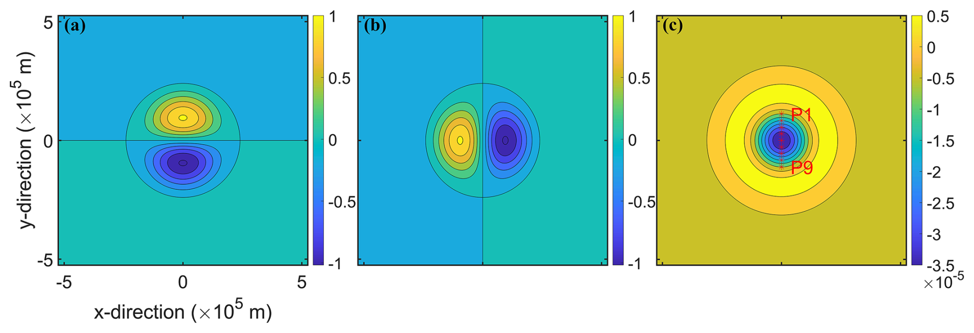
Figure 4 Distributions of (a) zonal (u) and (b) meridional (v) components (m s⁻¹) of currents and (c) relative vorticity (s⁻¹) for an idealized anticyclonic eddy with a radius of 120 km. Model results at nine fixed locations (P1–P9) denoted by red asterisks along the y axis in (c) are examined.

Jing et al. (2017) proposed a method to calculate the efficiency of energy transfer from background mesoscale eddies to wind-induced NICs. In this study, we use the differences in the average speeds of NICs between the modified and original model (NICs_U_AE and NICs_U_CE) as proxies for the near-inertial energy generated in the mesoscale eddies by the interaction between mesoscale eddies and NICs:

$$\begin{array}{}\text{(22)}& {\displaystyle }\mathrm{NICs}\mathrm{\_}{\mathrm{U}}_{\mathrm{AE}}=\mathrm{NICs}\mathrm{\_}{\mathrm{U}}_{\mathrm{AE}}^{\mathrm{Modified}}-\mathrm{NICs}\mathrm{\_}{\mathrm{U}}_{\mathrm{AE}}^{\mathrm{Original}},\text{(23)}& {\displaystyle }\mathrm{NICs}\mathrm{\_}{\mathrm{U}}_{\mathrm{CE}}=\mathrm{NICs}\mathrm{\_}{\mathrm{U}}_{\mathrm{CE}}^{\mathrm{Modified}}-\mathrm{NICs}\mathrm{\_}{\mathrm{U}}_{\mathrm{CE}}^{\mathrm{Original}},\end{array}$$

where $\mathrm{NICs}\mathrm{\_}{\mathrm{U}}_{\mathrm{AE}}^{\mathrm{Modified}}$ ($\mathrm{NICs}\mathrm{\_}{\mathrm{U}}_{\mathrm{AE}}^{\mathrm{Original}}$) and $\mathrm{NICs}\mathrm{\_}{\mathrm{U}}_{\mathrm{CE}}^{\mathrm{Modified}}$ ($\mathrm{NICs}\mathrm{\_}{\mathrm{U}}_{\mathrm{CE}}^{\mathrm{Original}}$) are the averaged speeds of NICs based on results produced by the modified (original) slab model in the anticyclonic eddies and cyclonic eddies over the same time period, respectively. It should be noted that the simulated NICs by the original slab model represent the near-inertial energy generated directly by the wind forcing. Therefore, after removing the generation of wind-induced NICs, the differences NICs_U_AE and NICs_U_CE represent the amplitudes of NICs transferred by interactions between mesoscale eddies and NICs in the anticyclonic eddies and the cyclonic eddies, respectively.

To quantify differences in the NICs transferred by background currents between the anticyclonic and cyclonic eddies, we introduce a simple parameter α, defined as

$$\begin{array}{}\text{(24)}& \mathit{\alpha }={\displaystyle \frac{\mathrm{NICs}\mathrm{\_}{\mathrm{U}}_{\mathrm{AE}}}{\mathrm{NICs}\mathrm{\_}{\mathrm{U}}_{\mathrm{CE}}}}.\end{array}$$

If α is larger than 1, it means that the anticyclonic eddy can transfer more NICs than a cyclonic eddy with the same strength.

5.2 Effect of wind speeds

The wind speed affects the energy input from the wind to the SML and therefore influences interaction between mesoscale eddies and NICs. To facilitate theoretical analysis and generate a reasonable magnitude of the NIC speeds, we conduct the numerical experiments using cyclonically rotating winds and anticyclonically rotating winds in the Northern Hemisphere with constant wind speed (A). The wind stress τ used in our sensitivity study takes a form as follows:

$$\begin{array}{}\text{(25)}& {\mathit{\tau }}_x\left(t\right)+i{\mathit{\tau }}_y\left(t\right)=A{e}^{iBt},\end{array}$$

where τ_x(t) and τ_y(t) are time-dependent zonal and meridional components of wind stress, and B is the wind rotation frequency. Positive wind rotation frequencies represent cyclonically rotating winds and negative wind rotation frequencies indicate anticyclonically rotating winds.

Five numerical experiments (ExpA1–5) are conducted with the background idealized mesoscale eddy moving westward with a translational speed of 8 cm s⁻¹. The |SLA_c| values of both anticyclonic and cyclonic eddies are set to 0.64 m in these five experiments. The integration duration of the numerical simulations is 3000 h. The speeds (A) of time-varying winds in these five experiments are set to 5, 10, 13, 15, and 20 m s⁻¹, corresponding to wind stress amplitudes of 0.038, 0.150, 0.282, 0.412, and 0.876 N m⁻², respectively. The wind forcing rotates cyclonically at the inertial frequency f. The conclusions drawn from the average and the sum of nine locations (P1–P9) are consistent.

For a cyclonic eddy with |SLA_c|=0.64 m, the averaged speeds of NICs converted from this cyclonic eddy at the abovementioned nine locations (NICs_U_CE) are about 1.01 × 10⁻³ m s⁻¹ and 2.32 × 10⁻² m s⁻¹ for cyclonic wind speeds of 5 m s⁻¹ (i.e., 0.038 N m⁻²) and 20 m s⁻¹ (i.e., 0.876 N m⁻²), respectively (Fig. 5a). This suggests that, within the cyclonic eddy, the NICs_U_CE increases 23 times if the cyclonic wind stress increases 23 times, which is consistent with the conclusion based on the analytical solution in Sect. 6.

In an anticyclonic eddy with the same strength of |SLA_c| = 0.64 m, the averaged speeds of NICs transferred from this anticyclonic eddy at the nine locations (NICs_U_AE) also increase with the wind speeds. The NICs_U_AE values are about 2.10 × 10⁻³ and 4.85 × 10⁻² m s⁻¹ for the cyclonic wind speeds of 5 m s⁻¹ (corresponding to 0.038 N m⁻²) and 20 m s⁻¹ (corresponding to 0.876 N m⁻²), respectively (Fig. 5a). This indicates that the averaged speeds of NICs generated in anticyclonic eddies by the interaction between background anticyclonic eddies and NICs also increase linearly with the cyclonic wind stress. But the NICs are stronger in the anticyclonic eddy than in the cyclonic eddy under the same wind conditions.

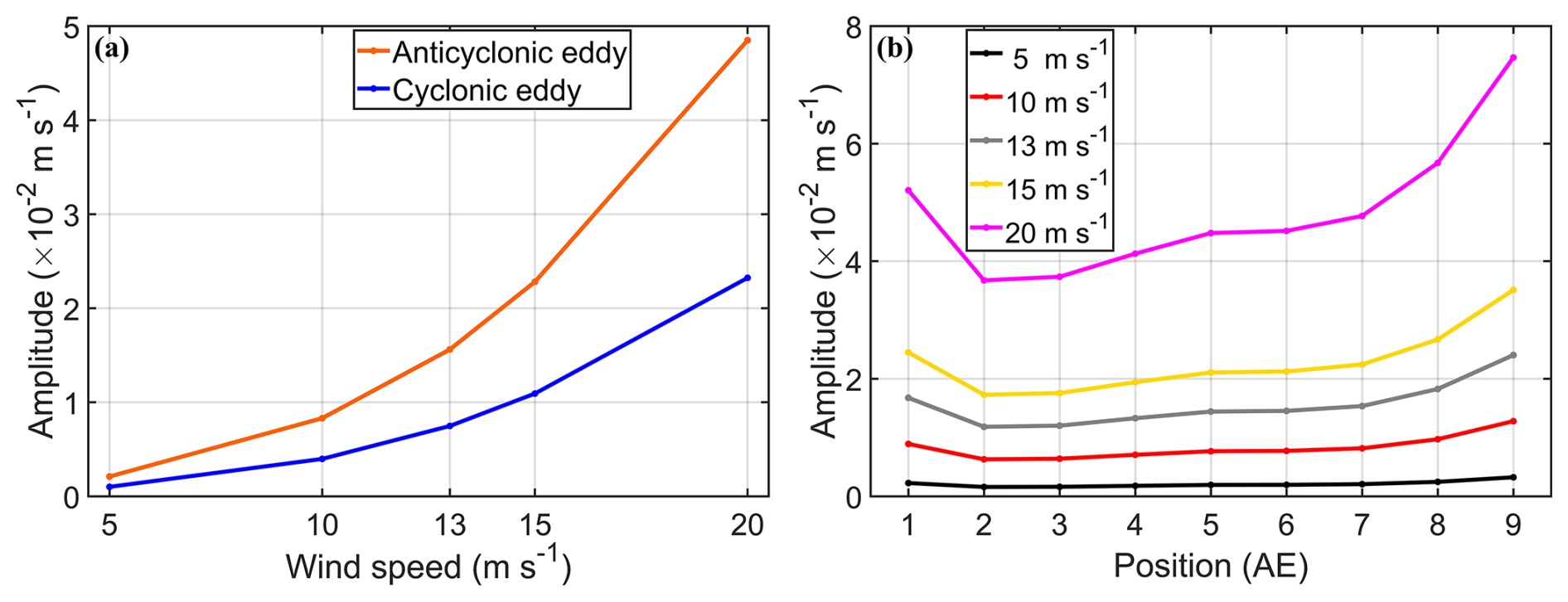
Figure 5 (a) Averaged speeds of transferred NICs at nine fixed locations, P1–P9, as a function of the wind speeds in the anticyclonic eddy (orange line) and cyclonic eddy (blue line), respectively. (b) Averaged speeds of transferred NICs as a function of the wind speeds in the anticyclonic eddy. The black, red, gray, yellow, and purple lines respectively indicate wind speeds of 5 m s⁻¹ (ExpA1), 10 m s⁻¹ (ExpA2), 13 m s⁻¹ (ExpA3), 15 m s⁻¹ (ExpA4), and 20 m s⁻¹ (ExpA5). Numbers on the horizontal axis in (b) denote nine fixed locations, P1 to P9. The wind rotates cyclonically at the inertial frequency. Mesoscale eddies move westward at the translational speed of 8 cm s⁻¹ and $\left|{\mathrm{SLA}}_{\mathrm{c}}\right|=\mathrm{0.64}$ m.

It should be noted, however, that the transferred near-inertial energy varies with the actual locations within the mesoscale eddy. We take the example of anticyclonic eddies to illustrate this issue. In anticyclonic eddies, the difference between the nine locations P1–P9 is large (Fig. 5b). The amplitude shows a distribution characterized by small values at the eddy center and relatively large values at the eddy edge, and this distribution characteristic is more obvious with the increase in the wind speed. The amplitudes of transferred NICs decrease outward from the eddy edge and are small in the rim of the mesoscale eddy.

The Okubo–Weiss parameter increases radially outward from the center of the mesoscale eddy. When the wind speed is relatively small, the difference of the energy generation induced by the Okubo–Weiss parameter is not significant (Fig. 5b). With the increase in the wind energy input, the larger absolute value of the positive Okubo–Weiss parameter gradually has the decisive function in the energy transfer. Therefore, it makes the anticyclonic eddy exhibit superior energy conversion characteristics at the eddy edge, which is consistent with the conclusion based on the energy transfer rate (Fig. 10).

The α values (Eq. 24) are about 2.08 based on the averaged speeds of NICs at the nine locations in the five different wind speeds. This indicates that the anticyclonic eddy is more efficient than the cyclonic eddy in transferring the kinetic energy to NICs (Fig. 5a). The difference in the near-inertial energy transfer efficiency between anticyclonic and cyclonic eddies is not affected very much by magnitudes of wind speeds.

5.3 Effect of wind rotation frequencies

The rotation frequency of the winds can affect the generation of the NICs and thus the energy transfer between the mesoscale eddy and NICs; therefore 28 numerical experiments using different wind rotation frequencies (±1.5f, ±1.25f, ±1.2f, ±1.15f, ±1.1f, ±1.05f, ±f, ±0.95f, ±0.9f, ±0.85f, ± 0.8f, ±0.75f, ±0.5f, and ±0.25f, where f is the inertial frequency), denoted as ExpB1–28, are conducted. Positive wind rotation frequencies correspond to cyclonically rotating winds, and negative wind rotation frequencies are for anticyclonically rotating winds. In these 28 experiments, the mesoscale eddy moves westward at the speed of 8 cm s⁻¹ and |SLA_c|=0.64 m. The winds rotate at different frequencies and the wind speed is set to 13 m s⁻¹.

Figure 6 shows the averaged speeds of the transferred NICs at the nine locations as a function of the wind rotation frequency for the cyclonic and anticyclonic eddies. Under cyclonically rotating and anticyclonically rotating wind conditions, there is bidirectional energy transfer between mesoscale eddies and NICs. The closer the absolute value of the wind rotation frequency to f, the stronger the energy transfer between mesoscale eddies and NICs. When the wind rotation frequency is negative, the wind rotation direction is the same as that of the local NICs. Wind rotation frequencies close to the inertial frequency of −f can lead to resonance and induce large NICs. Therefore, strong NICs provide a significant energy source for reverse energy conversion, allowing the near-inertial kinetic energy to be reabsorbed into the background mesoscale eddies and contribute to the reconstruction of the geostrophic balance.

For cyclonic eddies, the averaged speeds of NICs (NICs_U_CE) are sensitive to the wind rotation frequency. The NICs_U_CE values are less than zero when the winds rotate cyclonically at frequencies of 0.25f, 0.75f, and 1.25f (Fig. 6b), and the winds rotate anticyclonically at frequencies ranging from −1.15f to −0.75f (Fig. 6a), indicating that the direction of the energy transfer is from the NICs to the cyclonic eddies. The amplitudes of the energy transferred from NICs to cyclonic eddies under anticyclonically rotating wind conditions are larger than those transferred under cyclonically rotating wind conditions. The addition of mesoscale eddies has a damping effect for NICs, leading to negative energy transfer that aligns with the observed results (Fig. 2). When the direction of the energy transfer is positive, the NICs_U_CE has a maximum value of about 7.05 × 10⁻² m s⁻¹ when the winds rotate anticyclonically at the frequency of −1.25f.

For anticyclonic eddies, the averaged speeds of NICs (NICs_U_AE) also vary with the wind rotating frequency. When the winds rotate anticyclonically at frequencies ranging from −1.5f to −0.9f, the direction of the energy transfer is from NICs to anticyclonic eddies (Fig. 6a). The negative energy transfer is strongest at the resonance frequency of −f. The NICs_U_AE values are all positive under cyclonically rotating winds, which represent the energy transfer from the anticyclonic eddies to NICs (Fig. 6b). The NICs_U_AE values for the anticyclonic eddies increase from the value of ∼ 2.49 × 10⁻⁴ m s⁻¹ at the wind rotating frequency of 0.25f to the maximum value of ∼ 2.37 × 10⁻² m s⁻¹ at the wind rotating frequency of 0.90f. The NICs_U_AE values are larger than the NICs_U_CE values under the same positive wind rotation frequency. The closer the rotational frequency of the cyclonic winds is to the inertial frequency, the greater the difference in near-inertial energy conversion induced by anticyclonic eddies and cyclonic eddies.

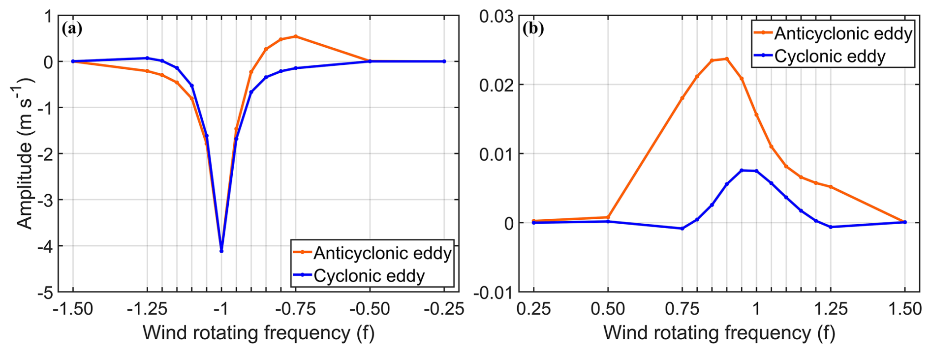
Figure 6 Averaged speeds of transferred NICs at nine fixed locations, P1–P9, as a function of rotation frequencies of (a) anticyclonically rotating winds and (b) cyclonically rotating winds. The orange and blue lines respectively indicate the anticyclonic eddy and cyclonic eddy. The wind rotation frequencies are normalized by the inertial frequency f.

5.4 Effect of eddy translational speeds

The translational speed of a background mesoscale eddy defines the forcing duration of winds and thus the energy input to NICs in the ocean SML. Based on the observations of mesoscale eddies in the nSCS, nine numerical experiments (ExpC1–9) using different translational speeds of mesoscale eddies (4, 5, 6, 7, 8, 9, 10, 11, and 12 cm s⁻¹) are conducted. In these nine experiments, the speed of cyclonically rotating winds at the inertial frequency is set to 13 m s⁻¹. The mesoscale eddy moves westward and |SLA_c|=0.64 m.

For the anticyclonic eddy with |SLA_c|=0.64 m, the average speeds of the converted NICs at the nine locations (NICs_U_AE) increase from about 1.48 × 10⁻² to 1.64 × 10⁻² m s⁻¹ as the translational speeds increase from 4 to 11 cm s⁻¹ (Fig. 7a). After the translational speed reaches 11 cm s⁻¹, the value of NICs_U_AE remains almost the same as that at a translational speed of 11 cm s⁻¹. The increase in the translational speed enhances the total kinetic energy of mesoscale eddies, which can provide a larger energy source and be more beneficial for the conversion of NICs. The translational speed of the mesoscale eddy is smaller than the maximum rotation speed of the mesoscale eddy, which is about 1.62 m s⁻¹ in this study. It should be noted that the change in the eddy kinetic energy caused by the different translational speeds is relatively small in comparison with the total eddy energy determined by the mesoscale eddy strength. Therefore, the change in the amplitude of the transferred NICs is relatively small.

For a cyclonic eddy with |SLA_c|=0.64 m, the average speeds of the transferred NICs at the nine locations (NICs_U_CE) range from 7.34 × 10⁻³ to 7.63 × 10⁻³ m s⁻¹ and are not sensitive to the translational speeds (Fig. 7a). As in the anticyclonic eddy case, more total kinetic energy is available for generating NICs within the cyclonic eddy with the same structure but with the faster translational speeds. Different from the anticyclonic eddy case, however, the cyclonic eddy is not conducive to energy transfer to NICs naturally. Therefore, the slightly larger energy source caused by the increase in the translational speeds has little influence on the total amount of kinetic energy transferred from the cyclonic eddy to NICs.

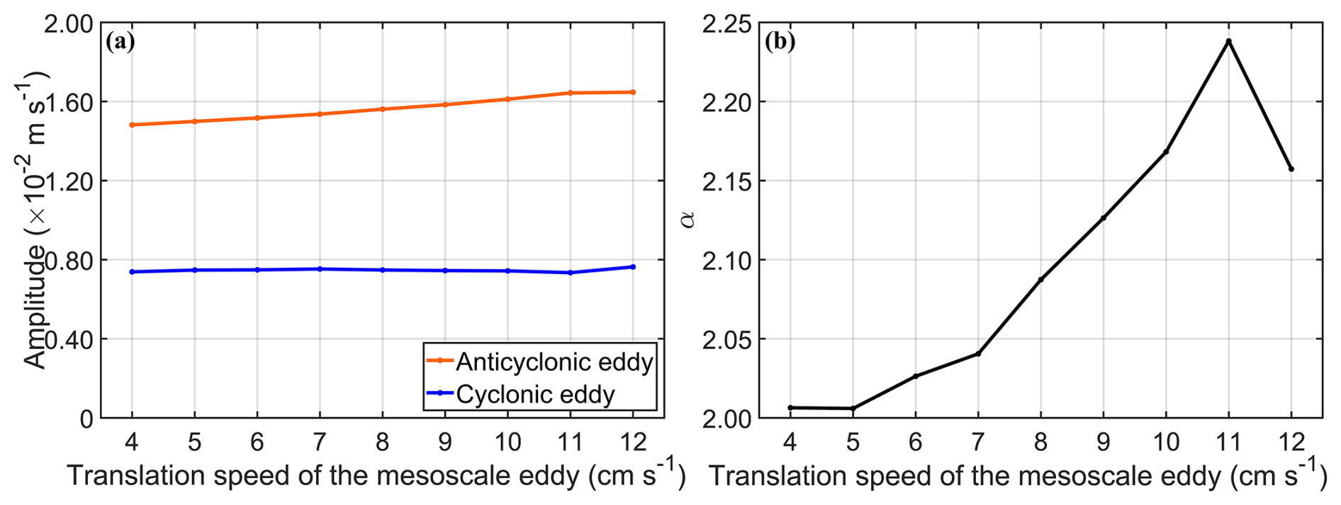
Figure 7 (a) Averaged speeds of transferred NICs at nine fixed locations, P1–P9, as a function of the eddy translational speed in the anticyclonic eddy (orange line) and cyclonic eddy (blue line), respectively. (b) The α value as a function of the eddy translational speed. The speed of the cyclonic wind is 13 m s⁻¹, and the wind rotates at the inertial frequency. Mesoscale eddies move westward and |SLA_c| =0.64 m.

The α value has a maximum of ∼ 2.24, occurring at eddy translational speeds of 11 cm s⁻¹ (Fig. 7b). This means that the anticyclonic eddy transfers much more near-inertial energy than the cyclonic eddy does, particularly at the translational speed of 11 cm s⁻¹. After exceeding the translational speed of 11 cm s⁻¹, the α values decrease with the increase in the eddy translational speeds. The α value is ∼ 2.16 at the translational speed of 12 cm s⁻¹. The average speeds of the NICs at the mesoscale eddy edge are generally larger than at the mesoscale eddy center.

A natural question is raised regarding whether the variations of α values within the mesoscale eddy are affected by the strength of anticyclonic eddies. To address this issue, we consider the averaged speeds of NICs at nine locations for mesoscale eddies and the α values with different strengths and translational speeds (Fig. 8). We consider the case with the cyclonically rotating wind speed of 13 m s⁻¹ at the inertial frequency. For mesoscale eddies with larger |SLA_c| values, the α values are relatively less sensitive to the translational speed. For mesoscale eddies with different |SLA_c| values, the α values all have the maximum values with the translational speeds of 11 cm s⁻¹. The α value decreases with the elevated translational speed when the eddy translational speed is larger than 11 cm s⁻¹.

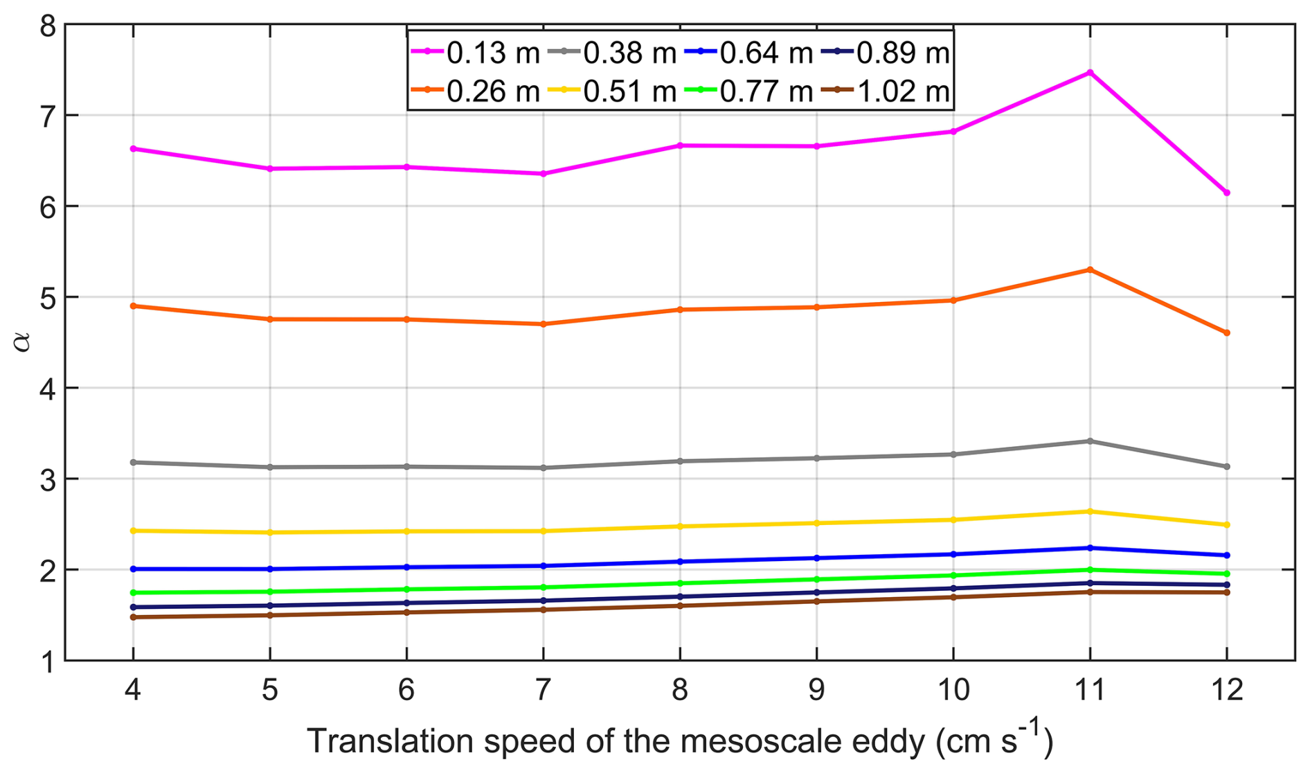
Figure 8 The α values at nine fixed locations, P1–P9, as a function of the strengths and translational speeds of the mesoscale eddies. The speed of the cyclonically rotating winds at the inertial frequency is 13 m s⁻¹. Mesoscale eddies move westward. Different colors of lines represent different mesoscale eddy strengths.

5.5 Effect of mesoscale eddy strengths

In addition to the effect of the eddy translational speed, other characteristics of mesoscale eddies such as the radius and strength of mesoscale eddies can also affect the energy exchange. A total of 16 numerical experiments (denoted as ExpD1–16) are conducted in this section using various strengths of mesoscale eddies. In these 16 experiments, the speed of cyclonically rotating winds at the inertial frequency is set to 13 m s⁻¹, the translational speed of mesoscale eddies is set to 8 cm s⁻¹, and the eddy translational direction is westward. The |SLA_c| values are set to 0.13, 0.26, 0.38, 0.51, 0.64, 0.77, 0.89, and 1.02 m for cyclonic and anticyclonic eddies.

Figure 9a shows the averaged speeds of the transferred NICs at nine locations as a function of the mesoscale eddy strengths for the cyclonic eddies (NICs_U_CE) and anticyclonic eddies (NICs_U_AE). Values of both NICs_U_CE and NICs_U_AE are larger for higher eddy strengths, particularly for the anticyclonic eddies. For the |SLA_c| values equal to 0.13 m, values of NICs_U_AE and NICs_U_CE are about 2.10 × 10⁻³ m s⁻¹ and about 3.15 × 10⁻⁴ m s⁻¹. The averaged speeds of the converted NICs increase with the |SLA_c| value, particularly for the anticyclonic eddies. For $\left|{\mathrm{SLA}}_{\mathrm{c}}\right|=\mathrm{1.02}$ m, the averaged speeds of the transferred NICs are ∼ 3.11 × 10⁻² and ∼ 1.94 × 10⁻² m s⁻¹ for the anticyclonic and cyclonic eddies, respectively, which are approximatively 15 times and approximatively 62 times larger than the counterparts at |SLA_c|=0.13 m. As the geostrophic strain field is relatively stronger at the eddy edge, the average speeds of the converted NICs at the mesoscale eddy edge are larger than at the mesoscale eddy center.

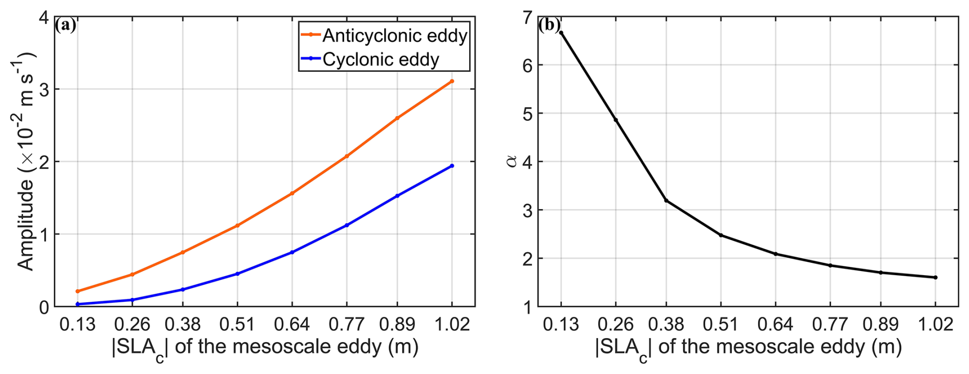
Figure 9 (a) Averaged speeds of transferred NICs at nine fixed locations, P1–P9, as a function of the strengths ($\left|{\mathrm{SLA}}_{\mathrm{c}}\right|$ of the mesoscale eddy) of the anticyclonic eddy (orange line) and cyclonic eddy (blue line). (b) The α value as a function of the eddy strengths ($\left|{\mathrm{SLA}}_{\mathrm{c}}\right|$ of the mesoscale eddy). The mesoscale eddy moves westward at the speed of 8 cm s⁻¹. The speed of the cyclonically rotating wind speed at the inertial frequency is set to 13 m s⁻¹.

The α value also varies with the mesoscale eddy strength (Fig. 9b). The α value decreases significantly from about 6.66 to 1.60 for |SLA_c| values in the range of 0.13 to 1.02 m. As mentioned above, cyclonic eddies have limited ability in transferring their kinetic energy to NICs, which differs significantly from anticyclonic eddies. However, stronger cyclonic eddies with more eddy energy provide the more favorable condition for energy transfer, which can narrow the difference in the near-inertial energy transfer induced by anticyclonic eddies and cyclonic eddies. Furthermore, stronger geostrophic currents lead to a stronger geostrophic strain field, which can generate stronger NICs.

5.6 Relative vorticity and strain

As mentioned above, the anticyclonic eddies in the SML are more efficient than cyclonic eddies for transferring kinetic energy to NICs, which can be explained by the relative vorticity of the background flow (ζ) defined in Eq. (1). In numerical experiments, the direction of the energy transfer is bidirectional but primarily positive – that is, from mesoscale eddies to NICs. For cyclonic eddies, the direction of the energy transfer is from the NICs to the cyclonic eddy under cyclonically rotating winds at frequencies of 0.25f, 0.75f, and 1.25f and anticyclonically rotating winds in a frequency range of −1.15f to −0.75f. When the frequencies of anticyclonically rotating winds range from −1.5f to −0.9f, the energy transfer is also negative in the anticyclonic eddy. The α value is more than 1.0 for about 87 % of these experiments, which indicates that the transferred near-inertial energy is larger in anticyclonic eddies than cyclonic eddies.

In addition to the relative vorticity and translational speed of a mesoscale eddy, the normal strain and shear strain of the background flow can also affect the energy transfer between the mesoscale eddy and NICs in the SML. Jing et al. (2017) proposed a method to calculate the rate of energy transfer from background mesoscale eddies to wind-induced NICs. Following Jing et al. (2017), the energy transfer rate (ε) between the NICs and the mesoscale eddy in the SML is given as

$$\begin{array}{}\text{(26)}& \mathit{\epsilon }=-\mathit{\rho }{H}_{\mathrm{mix}}\left(uu{U}_x+uv{U}_y+uv{U}_x+vv{V}_y\right),\end{array}$$

where u and v are respectively the zonal and meridional components of the near-inertial current velocity reproduced by the modified slab model, and subscripts x and y in U and V represent partial derivatives. The positive ε values mean the energy transfer from the mesoscale eddy to the NICs, and the negative ε indicates the backward energy cascade. In the numerical experiments, the NICs can be generated directly by the cyclonic winds, and the wind-induced NICs can further interact with the mesoscale eddy and transfer the near-inertial energy from the mesoscale eddy to the NICs when the mesoscale eddy passes by the nine locations P1–P9. Therefore, we also calculate the energy transfer rate and Okubo–Weiss parameter at the nine fixed locations P1–P9 in the sensitivity experiments ExpA3, ExpC1–C9, and ExpD1–D16, which are under the same wind conditions.

When the Okubo–Weiss parameters (strains) are negative, the energy transfer rate decreases as the Okubo–Weiss parameter (strain) increases (Fig. 10). However, when the Okubo–Weiss parameters (strains) are positive, the energy transfer rate shows an elevated trend with the increase in the Okubo–Weiss parameter (strain). Based on limited sensitivity studies, we found that the relative vorticity and the strain of the mesoscale eddy both have an influence on the near-inertial energy transferred by interactions between mesoscale eddies and NICs.

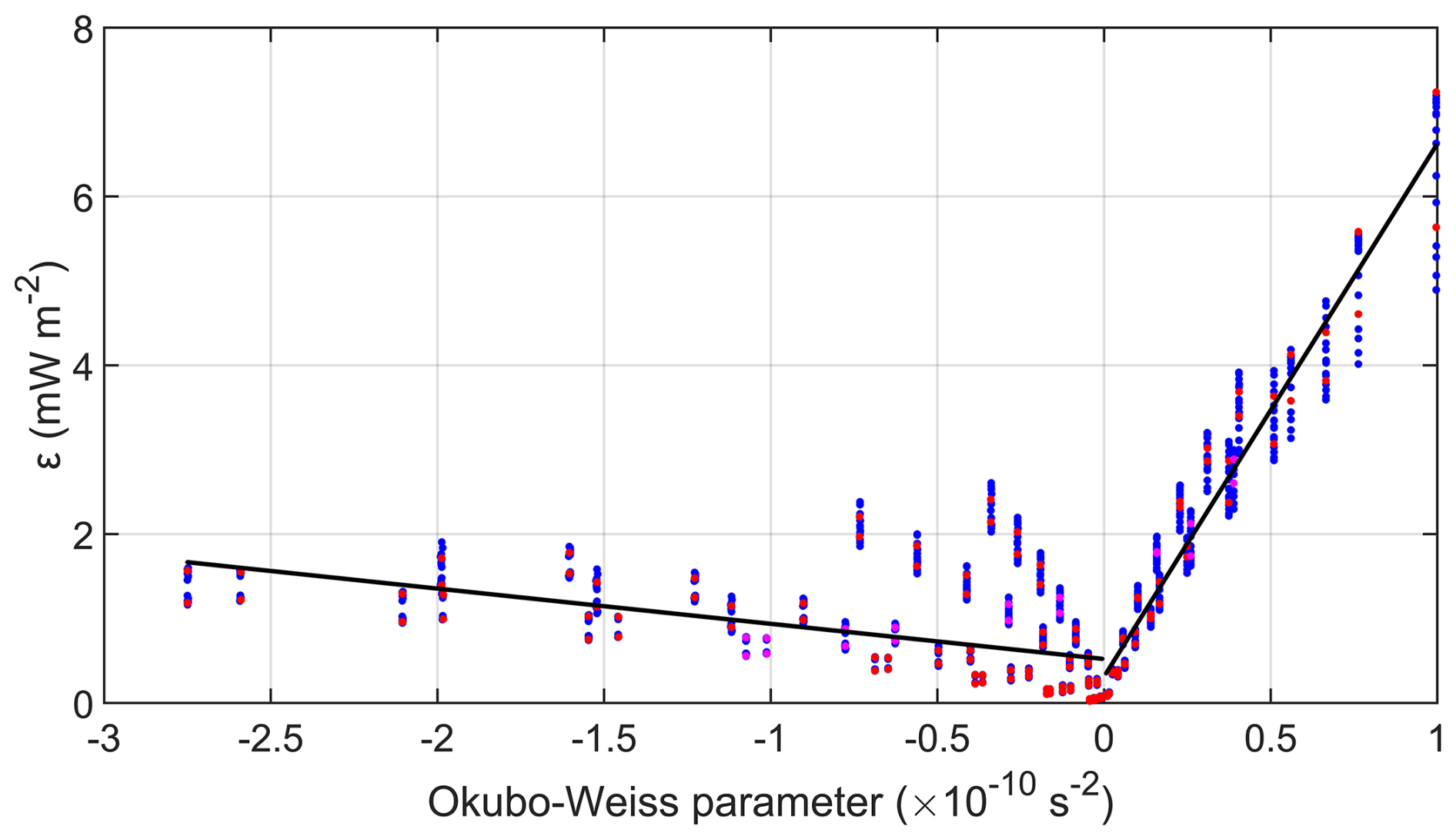
Figure 10 Scatterplot of the energy transfer rate and the Okubo–Weiss parameter. Purple, blue, and red dots respectively represent ExpA3, ExpC1–9, and ExpD1–16. The left (right) black line is the linear fitting line when the Okubo–Weiss parameters are negative (positive).

6 Theoretical analyses

6.1 Solutions in the frequency domain

To gain a better understanding of the role of the relative vorticity in the background flow for anticyclonic eddies to be significantly more efficient than the cyclonic eddies in transferring their kinetic energy to NICs, we analytically examine the effect of the relative vorticity in the frequency domain solution of the modified slab model.

The modified slab model can be written in the tensor form:

$$\begin{array}{}\text{(27)}& {\displaystyle \frac{\partial }{\partial t}}\left\{\begin{array}{c}u\\ v\end{array}\right\}+\left[\begin{array}{cc}{a}_{\mathrm{1}}& b_{\mathrm{1}}\\ a_{\mathrm{2}}& b_{\mathrm{2}}\end{array}\right]\left\{\begin{array}{c}u\\ v\end{array}\right\}=\left\{\begin{array}{c}{c}_{\mathrm{1}}\\ c_{\mathrm{2}}\end{array}\right\},\end{array}$$

where $a_{\mathrm{1}}=U_x+r$, $a_{\mathrm{2}}=V_x+f$, $b_{\mathrm{1}}=U_y-f$, $b_{\mathrm{2}}=V_y+r$, $c_{\mathrm{1}}={\mathit{\tau }}_x/\mathit{\rho }{H}_{\mathrm{mix}}$, and $c_{\mathrm{2}}={\mathit{\tau }}_y/\mathit{\rho }{H}_{\mathrm{mix}}$. Under steady winds, the NICs produced by the original slab model are zero; therefore the NICs produced by the modified slab model directly represent the near-inertial energy converted between mesoscale eddies and NICs. For simplicity, we consider the steady wind forcing to directly eliminate the wind-induced NICs here. In the case of steady winds, we use the Fourier transform to translate the modified slab model from the time domain into the frequency domain:

$$\begin{array}{}\text{(28)}& \left[\begin{array}{cc}{a}_{\mathrm{1}}+i\mathit{\omega }& b_{\mathrm{1}}\\ a_{\mathrm{2}}& b_{\mathrm{2}}+i\mathit{\omega }\end{array}\right]\left\{\begin{array}{c}\stackrel{\mathrm{̃}}{u}\\ \stackrel{\mathrm{̃}}{v}\end{array}\right\}=\left\{\begin{array}{c}\stackrel{\mathrm{̃}}{c_{\mathrm{1}}}\\ \stackrel{\mathrm{̃}}{c_{\mathrm{2}}}\end{array}\right\},\end{array}$$

where ω is the frequency and variables with a tilde represent the values after Fourier transform.

Assuming the mesoscale eddy is in an almost steady state during an inertial period (Jing et al., 2017), the analytical solution for the zonal and meridional components of NICs in the frequency domain can be written as

$$\begin{array}{}\text{(29)}& {\displaystyle }\stackrel{\mathrm{̃}}{u}={\displaystyle \frac{\left(b_{\mathrm{2}}+i\mathit{\omega }\right)\cdot \mathrm{2}\cdot \mathit{\pi }\cdot c_{\mathrm{1}}\cdot \mathit{\delta }\left(\mathit{\omega }\right)-b_{\mathrm{1}}\cdot \mathrm{2}\cdot \mathit{\pi }\cdot c_{\mathrm{2}}\cdot \mathit{\delta }\left(\mathit{\omega }\right)}{\left(a_{\mathrm{1}}+i\mathit{\omega }\right)\left(b_{\mathrm{2}}+i\mathit{\omega }\right)-a_{\mathrm{2}}{b}_{\mathrm{1}}}},\text{(30)}& {\displaystyle }\stackrel{\mathrm{̃}}{v}={\displaystyle \frac{\left(a_{\mathrm{1}}+i\mathit{\omega }\right)\cdot \mathrm{2}\cdot \mathit{\pi }\cdot c_{\mathrm{2}}\cdot \mathit{\delta }\left(\mathit{\omega }\right)-a_{\mathrm{2}}\cdot \mathrm{2}\cdot \mathit{\pi }\cdot c_{\mathrm{1}}\cdot \mathit{\delta }\left(\mathit{\omega }\right)}{\left(a_{\mathrm{1}}+i\mathit{\omega }\right)\left(b_{\mathrm{2}}+i\mathit{\omega }\right)-a_{\mathrm{2}}{b}_{\mathrm{1}}}},\end{array}$$

where δ(ω) is the Dirac delta function.

Based on Parseval's theorem, the energy of NICs is the same in both the time and frequency domains:

$$\begin{array}{}\text{(31)}& {\displaystyle \frac{\mathrm{1}}{T}}\int {\left|U\left(t\right)\right|}^{\mathrm{2}}\mathrm{d}t=\int {\left|U\left(\mathit{\omega }\right)\right|}^{\mathrm{2}}\mathrm{d}\mathit{\omega },\end{array}$$

where T is the total period.

The time mean near-inertial kinetic energy $\stackrel{\mathrm{‾}}{U_{{\mathrm{NIW}}_{\mathrm{s}}}^{\mathrm{2}}}$ in the time domain can be written as

$$\begin{array}{}\text{(32)}& {\displaystyle }\stackrel{\mathrm{‾}}{U_{{\mathrm{NIW}}_{\mathrm{s}}}^{\mathrm{2}}}=\stackrel{\mathrm{‾}}{u^{\mathrm{2}}}+\stackrel{\mathrm{‾}}{v^{\mathrm{2}}},\text{(33)}& {\displaystyle }\stackrel{\mathrm{‾}}{u^{\mathrm{2}}}=\int {\displaystyle \frac{\left({\left(b_{\mathrm{2}}{c}_{\mathrm{1}}-b_{\mathrm{1}}{c}_{\mathrm{2}}\right)}^{\mathrm{2}}+{\mathit{\omega }}^{\mathrm{2}}{c}_{\mathrm{1}}^{\mathrm{2}}\right)\cdot \left({\left(\mathrm{2}\cdot \mathit{\pi }\cdot \mathit{\delta }\left(\mathit{\omega }\right)\right)}^{\mathrm{2}}\right)}{{\left(a_{\mathrm{2}}{b}_{\mathrm{1}}-a_{\mathrm{1}}{b}_{\mathrm{2}}+{\mathit{\omega }}^{\mathrm{2}}\right)}^{\mathrm{2}}+{\mathit{\omega }}^{\mathrm{2}}{\left(a_{\mathrm{1}}+b_{\mathrm{2}}\right)}^{\mathrm{2}}}}\cdot \mathrm{d}\mathit{\omega },\text{(34)}& {\displaystyle }\stackrel{\mathrm{‾}}{v^{\mathrm{2}}}=\int {\displaystyle \frac{\left({\left(a_{\mathrm{1}}{c}_{\mathrm{2}}-a_{\mathrm{2}}{c}_{\mathrm{1}}\right)}^{\mathrm{2}}+{\mathit{\omega }}^{\mathrm{2}}{c}_{\mathrm{2}}^{\mathrm{2}}\right)\cdot \left({\left(\mathrm{2}\cdot \mathit{\pi }\cdot \mathit{\delta }\left(\mathit{\omega }\right)\right)}^{\mathrm{2}}\right)}{{\left(a_{\mathrm{2}}{b}_{\mathrm{1}}-a_{\mathrm{1}}{b}_{\mathrm{2}}+{\mathit{\omega }}^{\mathrm{2}}\right)}^{\mathrm{2}}+{\mathit{\omega }}^{\mathrm{2}}{\left(a_{\mathrm{1}}+b_{\mathrm{2}}\right)}^{\mathrm{2}}}}\cdot \mathrm{d}\mathit{\omega }.\end{array}$$

For a unidirectional laterally sheared geostrophic flow and southwestward wind, U=0, V=V(x), c₁<0, and c₂<0. Substitution of a₁=r, $a_{\mathrm{2}}=\mathit{\zeta }+f$, $b_{\mathrm{1}}=-f$, and b₂=r into Eqs. (33) and (34) yields

$$\begin{array}{}\text{(35)}& {\displaystyle }\stackrel{\mathrm{‾}}{u^{\mathrm{2}}}=\int {\displaystyle \frac{\left({\left(r{c}_{\mathrm{1}}+f{c}_{\mathrm{2}}\right)}^{\mathrm{2}}+{\mathit{\omega }}^{\mathrm{2}}{c}_{\mathrm{1}}^{\mathrm{2}}\right)\left({\left(\mathrm{2}\cdot \mathit{\pi }\cdot \mathit{\delta }\left(\mathit{\omega }\right)\right)}^{\mathrm{2}}\right)}{{\left(r^{\mathrm{2}}-{\mathit{\omega }}^{\mathrm{2}}+f\left(\mathit{\zeta }+f\right)\right)}^{\mathrm{2}}+\mathrm{4}{\mathit{\omega }}^{\mathrm{2}}{r}^{\mathrm{2}}}}\mathrm{d}\mathit{\omega },\text{(36)}& {\displaystyle }\stackrel{\mathrm{‾}}{v^{\mathrm{2}}}=\int {\displaystyle \frac{\left({\left(r{c}_{\mathrm{2}}-\left(\mathit{\zeta }+f\right)c_{\mathrm{1}}\right)}^{\mathrm{2}}+{\mathit{\omega }}^{\mathrm{2}}{c}_{\mathrm{2}}^{\mathrm{2}}\right)\left({\left(\mathrm{2}\cdot \mathit{\pi }\cdot \mathit{\delta }\left(\mathit{\omega }\right)\right)}^{\mathrm{2}}\right)}{{\left(r^{\mathrm{2}}-{\mathit{\omega }}^{\mathrm{2}}+f\left(\mathit{\zeta }+f\right)\right)}^{\mathrm{2}}+\mathrm{4}{\mathit{\omega }}^{\mathrm{2}}{r}^{\mathrm{2}}}}\mathrm{d}\mathit{\omega }.\end{array}$$

Since the relative vorticity is negative in anticyclonic eddies, the denominator term for $\stackrel{\mathrm{‾}}{u^{\mathrm{2}}}$ in Eq. (35) is less than the value with positive relative vorticity. Therefore, the value of $\stackrel{\mathrm{‾}}{u^{\mathrm{2}}}$ is greater in anticyclonic eddies than in cyclonic eddies. For the positive relative vorticity, the numerator term of $\stackrel{\mathrm{‾}}{v^{\mathrm{2}}}$ is smaller and the denominator term in Eq. (36) becomes larger than the case of negative vorticity. This indicates that $\stackrel{\mathrm{‾}}{v^{\mathrm{2}}}$ is more elevated in the anticyclonic eddies. Since both $\stackrel{\mathrm{‾}}{u^{\mathrm{2}}}$ and $\stackrel{\mathrm{‾}}{v^{\mathrm{2}}}$ are more elevated when the relative vorticity is negative than counterparts with positive relative vorticity, anticyclonic eddies can transfer more near-inertial energy than cyclonic eddies.

6.2 Analytical solution

An analytical solution based on the modified slab model is considered here to demonstrate that mesoscale eddies can transfer more near-inertial energy for stronger winds. The modified slab model cane be written as

$$\begin{array}{}\text{(37)}& {\displaystyle \frac{\partial u}{\partial t}}+a_{\mathrm{1}}u+b_{\mathrm{1}}v=c_{\mathrm{1}},\text{(38)}& {\displaystyle \frac{\partial v}{\partial t}}+a_{\mathrm{2}}u+b_{\mathrm{2}}v=c_{\mathrm{2}},\end{array}$$

where, $a_{\mathrm{1}}=U_x+r$, $a_{\mathrm{2}}=V_x+f$, $b_{\mathrm{1}}=U_y-f$, $b_{\mathrm{2}}=V_y+r$, $c_{\mathrm{1}}={\mathit{\tau }}_x/\mathit{\rho }{H}_{\mathrm{mix}}$, $c_{\mathrm{2}}={\mathit{\tau }}_y/\mathit{\rho }{H}_{\mathrm{mix}}$, τ_x=Acos ft, and τ_y=Asin ft.

For the cyclonic wind, substitution of Eq. (37) into Eq. (38) yields

$$\begin{array}{}\text{(39)}& {\displaystyle }\begin{array}{rl}& {\displaystyle \frac{{\partial }^{\mathrm{2}}u}{\partial t^{\mathrm{2}}}}+\left(a_{\mathrm{1}}+b_{\mathrm{2}}\right){\displaystyle \frac{\partial u}{\partial t}}+\left(a_{\mathrm{1}}{b}_{\mathrm{2}}-a_{\mathrm{2}}{b}_{\mathrm{1}}\right)u\\ & =b_{\mathrm{2}}{c}_{\mathrm{1}}-(f+b_{\mathrm{1}})c_{\mathrm{2}},\end{array}\text{(40)}& {\displaystyle }\mathrm{\Delta }={\left(a_{\mathrm{1}}+b_{\mathrm{2}}\right)}^{\mathrm{2}}-\mathrm{4}\left(a_{\mathrm{1}}{b}_{\mathrm{2}}-a_{\mathrm{2}}{b}_{\mathrm{1}}\right).\end{array}$$

The analytical solutions of the current to the modified slab model are

$$\begin{array}{}\text{(41)}& {\displaystyle }\begin{array}{rl}{u}_{\mathrm{Modified}}& =e^{\mathit{\gamma }t}\left(Q_{\mathrm{1}}\cos \mathit{\beta }t+Q_{\mathrm{2}}\sin \mathit{\beta }t\right)\\ & +Q_{\mathrm{3}}\cos ft+Q_{\mathrm{4}}\sin ft,\\ v_{\mathrm{Modified}}& ={\displaystyle \frac{\mathrm{1}}{b_{\mathrm{1}}}}(c_{\mathrm{1}}-e^{\mathit{\gamma }t}\left(a_{\mathrm{1}}+\mathit{\gamma }\right)\\ & \left(Q_{\mathrm{1}}\cos \mathit{\beta }t+Q_{\mathrm{2}}\sin \mathit{\beta }t\right),\end{array}\text{(42)}& {\displaystyle }\begin{array}{rl}& -e^{\mathit{\gamma }t}\mathit{\beta }\left(Q_{\mathrm{2}}\cos \mathit{\beta }t-Q_{\mathrm{1}}\sin \mathit{\beta }t\right)\\ & +\left(f{Q}_{\mathrm{3}}-a_{\mathrm{1}}{Q}_{\mathrm{4}}\right)\sin ft-\left(f{Q}_{\mathrm{4}}+a_{\mathrm{1}}{Q}_{\mathrm{3}}\right)\cos ft),\end{array}\end{array}$$

where

$$\begin{array}{}\text{(43)}& {\displaystyle }\mathit{\gamma }=-{\displaystyle \frac{a_{\mathrm{1}}+b_{\mathrm{2}}}{\mathrm{2}}},\text{(44)}& {\displaystyle }\mathit{\beta }={\displaystyle \frac{\sqrt{-\mathrm{\Delta }}}{\mathrm{2}}},\text{(45)}& {\displaystyle }{Q}_{\mathrm{1}}=-Q_{\mathrm{3}},\text{(46)}& {\displaystyle }{Q}_{\mathrm{2}}={\displaystyle \frac{c_{\mathrm{1}}+\mathit{\gamma }{Q}_{\mathrm{3}}-f{Q}_{\mathrm{4}}}{\mathit{\beta }}},\text{(47)}& {\displaystyle }{Q}_{\mathrm{3}}={\displaystyle \frac{A{b}_{\mathrm{2}}\left(a_{\mathrm{1}}{b}_{\mathrm{2}}-a_{\mathrm{2}}{b}_{\mathrm{1}}-f^{\mathrm{2}}\right)+A(f+b_{\mathrm{1}})(f{a}_{\mathrm{1}}+f{b}_{\mathrm{2}})}{\mathit{\rho }{H}_{\mathrm{mix}}({\left(a_{\mathrm{1}}{b}_{\mathrm{2}}-a_{\mathrm{2}}{b}_{\mathrm{1}}-f^{\mathrm{2}}\right)}^{\mathrm{2}}+(f{a}_{\mathrm{1}}+f{b}_{\mathrm{2}}{)}^{\mathrm{2}})}},\text{(48)}& {\displaystyle }{Q}_{\mathrm{4}}={\displaystyle \frac{\mathit{\rho }{H}_{\mathrm{mix}}{Q}_{\mathrm{3}}(f{a}_{\mathrm{1}}+f{b}_{\mathrm{2}})-A(f+b_{\mathrm{1}})}{\mathit{\rho }{H}_{\mathrm{mix}}\left(a_{\mathrm{1}}{b}_{\mathrm{2}}-a_{\mathrm{2}}{b}_{\mathrm{1}}-f^{\mathrm{2}}\right)}}.\end{array}$$

Increasing the wind stress c₁ and c₂ by a factor of n named $c_{\mathrm{1}}^{\prime }$ and $c_{\mathrm{2}}^{\prime }$ yields

$$\begin{array}{}\text{(49)}& {\displaystyle }{c}_{\mathrm{1}}^{\prime }=n{c}_{\mathrm{1}}={\displaystyle \frac{n{\mathit{\tau }}_x}{\mathit{\rho }{H}_{\mathrm{mix}}}}={\displaystyle \frac{nA\cos ft}{\mathit{\rho }{H}_{\mathrm{mix}}}},\text{(50)}& {\displaystyle }{c}_{\mathrm{2}}^{\prime }=n{c}_{\mathrm{2}}={\displaystyle \frac{n{\mathit{\tau }}_y}{\mathit{\rho }{H}_{\mathrm{mix}}}}={\displaystyle \frac{nA\sin ft}{\mathit{\rho }{H}_{\mathrm{mix}}}}.\end{array}$$

Substitution of $c_{\mathrm{1}}^{\prime }$ and $c_{\mathrm{2}}^{\prime }$ into Q₃ and Q₄ yields

$$\begin{array}{}\text{(51)}& {\displaystyle }\begin{array}{rl}& Q_{\mathrm{3}}^{\prime }=\\ & {\displaystyle \frac{nA{b}_{\mathrm{2}}\left(a_{\mathrm{1}}{b}_{\mathrm{2}}-a_{\mathrm{2}}{b}_{\mathrm{1}}-f^{\mathrm{2}}\right)+nA(f+b_{\mathrm{1}})(f{a}_{\mathrm{1}}+f{b}_{\mathrm{2}})}{\mathit{\rho }{H}_{\mathrm{mix}}({\left(a_{\mathrm{1}}{b}_{\mathrm{2}}-a_{\mathrm{2}}{b}_{\mathrm{1}}-f^{\mathrm{2}}\right)}^{\mathrm{2}}+(f{a}_{\mathrm{1}}+f{b}_{\mathrm{2}}{)}^{\mathrm{2}})}}\\ & =n{Q}_{\mathrm{3}},\end{array}\text{(52)}& {\displaystyle }{Q}_{\mathrm{4}}^{\prime }={\displaystyle \frac{\mathit{\rho }{H}_{\mathrm{mix}}n{Q}_{\mathrm{3}}(f{a}_{\mathrm{1}}+f{b}_{\mathrm{2}})-nA(f+b_{\mathrm{1}})}{\mathit{\rho }{H}_{\mathrm{mix}}\left(a_{\mathrm{1}}{b}_{\mathrm{2}}-a_{\mathrm{2}}{b}_{\mathrm{1}}-f^{\mathrm{2}}\right)}}=n{Q}_{\mathrm{4}}.\end{array}$$

Substitution of Q₃ and Q₄ into Q₁ and Q₂ yields

$$\begin{array}{}\text{(53)}& {\displaystyle }{Q}_{\mathrm{1}}^{\prime }=-n{Q}_{\mathrm{3}}=n{Q}_{\mathrm{1}},\text{(54)}& {\displaystyle }{Q}_{\mathrm{2}}^{\prime }={\displaystyle \frac{n{c}_{\mathrm{1}}+\mathit{\gamma }n{Q}_{\mathrm{3}}-fn{Q}_{\mathrm{4}}}{\mathit{\beta }}}=n{Q}_{\mathrm{2}}.\end{array}$$

Therefore, the current with the increased wind stress to the modified slab model is given as

$$\begin{array}{}\text{(55)}& {\displaystyle }{u}_{\mathrm{Modified}}^{\prime }=n{u}_{\mathrm{Modified}},\text{(56)}& {\displaystyle }{v}_{\mathrm{Modified}}^{\prime }=n{v}_{\mathrm{Modified}}.\end{array}$$

The analytical solution of the current to the original slab model is

$$\begin{array}{}\text{(57)}& \begin{array}{rl}{U}_{\mathrm{Original}}& ={\displaystyle \frac{A{e}^{ift}}{\mathit{\rho }{H}_{\mathrm{mix}}(if+r)}}+\left(\left({\displaystyle \frac{A{e}^{-\left(if+r\right)t}}{\mathit{\rho }{H}_{\mathrm{mix}}\left(if+r\right)}}\right)\right.\\ & \left.\left({\displaystyle \frac{if}{\mathrm{2}if+r}}\right)\left(\mathrm{1}-e^{\left(\mathrm{2}if+r\right)t}\right)\right)-{\displaystyle \frac{A{e}^{-\left(if+r\right)t}}{\mathit{\rho }{H}_{\mathrm{mix}}\left(if+r\right)}}.\end{array}\end{array}$$

Therefore, the current with the increased wind stress to the original slab model is given as

$$\begin{array}{}\text{(58)}& U_{\mathrm{Original}}^{\prime }=n{U}_{\mathrm{Original}}.\end{array}$$

The above analytical solutions demonstrate that when the wind stress increases by n times, the current speeds simulated by the modified and original slab models both increase by n times. The differences in the average speeds of NICs between the modified and original model represent the transferred near-inertial energy by the interaction between mesoscale eddies and near-inertial motions (Eqs. 22 and 23). As the NICs are the component of the total currents in the near-inertial frequency band, the transferred near-inertial energy in the mesoscale eddies also increases by a factor of n times when the wind stress is multiplied by n times. This feature is consistent with our sensitivity experiments in Sect. 5.

7 Summary and discussion

Analysis of in situ current observations at two offshore ADCP mooring sites in the northern South China Sea (nSCS) demonstrated that relatively strong near-inertial currents (NICs) occurred during certain periods of nearly steady winds in the lower part of the ocean surface mixed layer (SML). The NICs produced by the original slab model are significantly larger than the observations, indicating other important processes operating over the area. We followed Weller (1982) and Jing et al. (2017) and used a modified slab model in this study by including contributions from the background geostrophic currents. Using the surface geostrophic currents inferred from the satellite sea level data and assuming that the geostrophic currents in the SML are vertically uniform, we found that the modified slab model performs significantly better than the original slab model in reproducing the observed NICs at two ADCP mooring sites in the nSCS. Examinations of observations and numerical results produced by the modified and original slab models revealed the occurrence of energy exchange between the mesoscale eddies and the NICs. Based on the energy budget analysis for NICs during the observational period, the difference of the near-inertial wind power input between the original slab model and the modified slab model is the same order as the energy transfer rate (Eq. 26). This also indicates the importance of the near-inertial energy transfer induced by the interaction between mesoscale eddies and NICs in the SML during the observational period.

The modified slab model and original slab model were then used to examine sensitivity to winds and eddy parameters with idealized mesoscale eddies under cyclonic winds. Both cyclonic and anticyclonic mesoscale eddies were considered, using the universal eddy structure suggested by Zhang et al. (2013). One of our major findings is that anticyclone eddies can transfer more kinetic energy to NICs than cyclonic eddies. Idealized experiments show that induced NIC speeds in anticyclonic eddies can reach over 6 times the speed in cyclonic eddies. We also found that the energy transfer rate is related to the Okubo–Weiss parameter. When the Okubo–Weiss parameter is positive, the energy transfer rate is elevated with the larger Okubo–Weiss parameter.

Analyses of model results in 226 numerical experiments using the modified slab model demonstrated that bidirectional energy transfer exists between mesoscale eddies and NICs. The direction of the energy transfer is primarily from mesoscale eddies to NICs. When the cyclonic winds rotate at frequencies of 0.25f, 0.75f, and 1.25f and the anticyclonic winds rotate at frequencies ranging from −1.15f to −0.75f, the direction of the energy transfer is negative in the cyclonic eddy – that is, from NICs to cyclonic eddies. Under anticyclonically rotating winds in the frequency range of −1.5f to −0.9f, negative energy transfer also occurs in the anticyclonic eddy. The NICs transferred from mesoscale eddies are stronger for higher wind speeds, faster translational speeds, and stronger strengths of mesoscale eddies. When the wind stress increases by a factor of n times, the amplitudes of the converted NICs are also multiplied by n times. The NICs transferred in mesoscale eddies by the interactions between mesoscale eddies and NICs are stronger for higher translational speeds of anticyclonic eddies. At translational speeds of 11 cm s⁻¹, the ratios of the amplitudes of the converted NICs by anticyclonic eddies to that transferred by cyclonic eddies reach maximum values.

For analytical considerations, the modified slab model was transferred from the time domain to the frequency domain using the Fourier transform. Using Parseval's theorem, we derived the time mean value of the induced NICs. The analytical expression was used to demonstrate that, for the negative relative vorticity, i.e., such as within an anticyclonic eddy, the transferred NICs are larger in an anticyclonic eddy than a cyclonic eddy. The analytical solution under the cyclonic winds also demonstrated that the NICs transferred by mesoscale eddies increase linearly with the wind stress. These analytical results are consistent with the results produced by the modified and original slab models.

We also conducted the same set of numerical experiments using steady winds with both constant speeds and direction, and model results in the steady winds are not presented here due to the page limit. Our main findings on the energy transfer between mesoscale eddies and NICs in these experiments with the steady winds are the same as the results using the rotating winds.

This study suggests that there is bidirectional energy transfer between mesoscale eddies and NICs in the SML, the mechanism and influence factors of which are further explored by idealized simulations. Our findings can further contribute to the understanding of the energy budget in the global ocean and the ocean response to climate change. In order to examine major physical processes affecting the NICs generated by mesoscale eddies and quantify their influence on turbulent mixing in the deeper ocean, further studies are needed using a three-dimensional ocean circulation model.