On the short-term response of entrained air bubbles in the upper ocean: a case study in the north Adriatic Sea

Air bubbles in the upper ocean are generated mainly by waves breaking at the air–sea interface. As such, after the waves break, entrained air bubbles evolve in the form of plumes in the turbulent flow, exchange gas with the surrounding water, and may eventually rise to the surface. To shed light on the short-term response of entrained bubbles in different stormy conditions and to assess the link between bubble plume penetration depth, mechanical and thermal forcings, and the air–sea transfer velocity of CO₂, a field experiment was conducted from an oceanographic research tower in the north Adriatic Sea. Air bubble plumes were observed using high-resolution echosounder data from an upward-looking 1000 kHz sonar. The backscatter signal strength was sampled at a high resolution, 0.5 s in time and 2.5 cm along the vertical direction. Time series profiles of the bubble plume depth were established using a variable threshold procedure applied to the backscatter strength. The data show the occurrence of bubbles organized into vertical plume-like structures, drawn downwards by wave-generated turbulence and other near-surface circulations, and reaching the seabed at 17 m depth under strong forcing. We verify that bubble plumes adapt rapidly to wind and wave conditions and have depths that scale approximately linearly with wind speed. Scaling with the wind–wave Reynolds number is also proposed to account for the sea-state severity in the plume depth prediction. Results show a correlation between measured bubble depths and theoretical air–sea CO₂ transfer velocity parametrized with wind-only and wind/wave formulations. Further, our measurements corroborate previous results suggesting that the sinking of newly formed cold-water masses helps bring bubbles to greater depths than those reached in stable conditions for the water column. The temperature difference between air and sea seems sufficient for describing this intensification at the leading order of magnitude. The results presented in this study are relevant for air–sea interaction studies and pave the way for progress in CO₂ gas exchange formulations.

1 Introduction

Air bubbles injected by breaking waves are ubiquitous in the upper layers of the global oceans. As such, when the wind blows over the sea above 3 m s⁻¹ and surface waves break entraining air, bubbles evolve in the upper-ocean turbulent flow and may eventually rise to the surface (Thorpe, 1992). This process controls the ventilation of the ocean and the uptake of less soluble gases from the atmosphere (Deike and Melville, 2018; IPCC, 2013; Kanwisher, 1963; Woolf, 1997). For CO₂, it has been estimated that the ocean is a sink for ∼ 25 % of the atmospheric gas emitted by human activities (Watson et al., 2020). During stormy conditions, a relevant part of the gas exchange is due to the bubble-mediated contribution (Reichl and Deike, 2020). The transfer of gases via bubbles depends on the depth/time history of the bubble plume, a multi-faceted process involving advection motion in the upper sea, the buoyancy of bubbles, hydrostatic pressure, and the net exchange of all gases (Woolf, 1997). For instance, in an early bubble advection model, the depth to which bubbles are carried is found to be proportional to the downward current component (Thorpe, 1982). The efficiency of the bubble-mediated transfer is controlled by the depth of the bubble penetration (Keeling, 1993), which has been incorporated in the latest bubble gas transfer models that parametrize the kinetic term of the CO₂ gas exchange as a function of both wind and wave forcings (Deike, 2022). Indirectly, the importance of understanding bubble depths is also relevant for estimating the energy dissipated by the whitecaps (Callaghan, 2018) that mediate the transfer of momentum from the atmosphere to the oceans (Cavaleri et al., 2012).

In situ bubble plumes can be measured using acoustic instruments, which were developed for military purposes during World War II and later adapted for scientific investigations of the near-surface aerated layer (Kanwisher, 1963; Medwin, 1970, 1977). Although at the time of writing, such type of measurements are relatively scarce, sonar observations of bubble plumes have made it possible to determine the local climatology of depths reached by bubbles and the relationship with surface forcings, primarily the wind speed (Cifuentes-Lorenzen et al., 2023; Derakhti et al., 2024; Graham et al., 2004; Strand et al., 2020; Thorpe and Stubbs, 1979; Vagle et al., 2010; Wang et al., 2016); accordingly, bubble depth has been described in the form of a linear dependency of type α(U−U_min), where U_min is the minimum speed U for detecting bubbles and α is assumed to be constant with wind speed. Studies show that under strong winds, bubbles are easily advected to depths of several tens of metres. The importance of sea-state severity and energy dissipation in determining the bubble production (Strand et al., 2020) and the dependence of bubble depth on sea states with different wave ages as a possible indicator of the breaking type have also been proved (Graham et al., 2004; Wang et al., 2016). Notwithstanding that Thorpe and Stubbs (1979) suggested that the shape and depth of the bubble plumes depend on the direction of heat fluxes through the water surface, their impact has been poorly investigated in later studies, which focussed only on the effect of surface wind and breaking waves on the bubble penetration.

The objective of this study is to characterize the short-term response of the bubble penetration in the upper ocean under different forcing mechanisms such as wind speed, wave field, and heat fluxes. The motivation is to provide elements to improve the current understanding of the bubble plume behaviour and its connection to air–sea gas transfer parametrization and modelling. As in previous studies, an upward-looking echo-sounding range instrument (sonar) was used to observe plumes of air bubbles, from the air–sea interface down to several metres below the surface. The sonar operated at a carrier frequency of 1000 kHz, which ensonified the small fraction of bubble sizes that could be treated as passive tracers for observing the processes in the near-surface mixed layer (Thorpe, 1992). Results are based on water and atmosphere observations collected from the Acqua Alta oceanographic research tower (Fig. 1). Acqua Alta is located at 45.31° N, 12.51° E, 15 km offshore the Venice littoral (Italy) in a relatively shallow (17 m deep) and gently sloping region of the north Adriatic Sea. The area is exposed to the open sea from the southeast (sirocco wind). By contrast, sea states from the northeast (bora wind) are generally fetch limited (the fetch is about 100 km). Further, mixed-wave conditions most likely occur when an energetic swell from the sirocco leaving the central part of the basin crosses locally generated wind waves from the northern quadrants, mainly from the northeast (Cavaleri, 1999). Relevant to the present study is that bora wind can bring cold and dry air, leading to intense sea surface heat fluxes, cooling of the water masses, and dense-water production with downward-moving waters (Benetazzo et al., 2014; Bergamasco et al., 1999; Bignami et al., 1990; Vilibić and Supić, 2005; Supić and Vilibić, 2006).

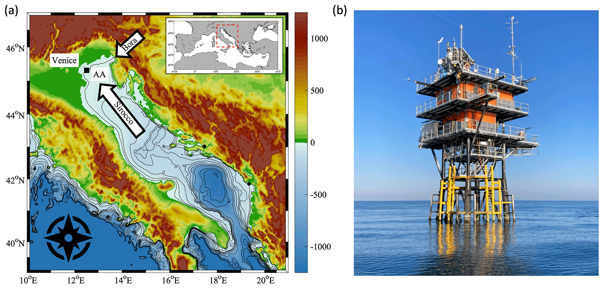
Figure 1 The experimental site. (a) The Adriatic Sea (bathymetry in blue shading from 0 to −1250 m), surrounding orography (green–brown shading), and location in the north of the Acqua Alta oceanographic research tower (AA label). The arrows sketch the directions of the typical northeasterly bora of the southeasterly sirocco winds. The inset shows the Mediterranean region with the Italian peninsula at its centre. (b) Lateral view of Acqua Alta (Photo credit: Francesco Barbariol).

We focus on analysing average and extreme bubble penetrations and their connection with wind and wind/wave parameters in the context of the formulae used to estimate the transfer velocity of CO₂ gas. In Sect. 2, we review the existing parametrizations that link bubble depth with wind speed and other forcing variables. In Sect. 3, the sonar observations during two storms in the north Adriatic Sea (the wind speed at 10 m reached 26 m s⁻¹ and the significant wave height of 3 m), the method used to compute the bubble depth, and the auxiliary observations used in this study are presented. The results are presented and discussed in Sect. 4. The main conclusions of the study are given in Sect. 5. An Appendix reviewing the existing formulae used to parametrize the transfer velocity of CO₂ gas completes the study.

2 Parametrization of the bubble plume penetration depth

In this section, we outline the parametrizations derived from experimental campaigns that provide the depth of air bubble plumes as a function of external and internal forcings. From early studies it became clear that the depth of bubble plumes increases monotonically with wind speed with a high correlation (Kanwisher, 1963). This evidence suggested finding an empirical law linking bubble depth to a reference wind speed, assuming that the wind must blow over a cut-off speed for air bubbles in the bulk of water. In most wind-speed ranges, the law was found to be linear.

The earliest empirical relationship was found by Thorpe and Stubbs (1979) in the freshwater of Loch Ness using records from a sonar moored at 30 m and operating at 248 kHz (the radius of resonating bubbles close to the surface is about 13 µm); these authors showed that bubbles are not detected for wind speed below U_min=2.5 m s⁻¹ and that the observed average penetration depth (z_ba, in m) of the bubble plumes increases linearly with the wind speed at 10 m height (U₁₀, in m s⁻¹), approximately as

$$\begin{array}{}\text{(1)}& z_{\text{ba}}=\mathrm{0.4}(U_{\mathrm{10}}-\mathrm{2.5}),\end{array}$$

which gives, for example z_ba=3 m (11 m) for U₁₀=10 m s⁻¹ (30 m s⁻¹). Thorpe and Stubbs (1979) recognized the relation between bubble plumes and turbulent structures within the near-surface mixing layer and that the plume variation could be associated with waves breaking in the area covered by the sonar. The authors also observed that the spatio-temporal shape of the plumes depends on the direction of the heat flux through the water surface: columnar plumes appeared when the air was colder than the water, and billow-like plumes were produced when the water was colder than the air. Hence, the bubble plumes and the thermal structure within the near-surface mixing layer are related.

The above consideration led Thorpe (1982) to include in Eq. (1) a parameter specifying the water column's stability and, hence, its ability to convey air bubbles further down when the surface water cools and water masses become denser and heavier. Since the air-minus-water temperature difference ΔT is a bulk indicator of the direction and intensity of the surface heat fluxes, the previous law was corrected for $\left|\mathrm{\Delta }T\right|<\mathrm{6}$ K as follows:

$$\begin{array}{}\text{(2)}& z_{\text{ba}}=\mathrm{0.31}{\mathrm{\Gamma }}_T(U_{\mathrm{10}}-\mathrm{2.5}),\end{array}$$

where

$$\begin{array}{}\text{(3)}& {\mathrm{\Gamma }}_T=(\mathrm{1}-\mathrm{0.1}\mathrm{\Delta }T)\end{array}$$

is a correction factor that accounts for the stability of the water column to temperature gradients. In unstable conditions, ΔT<0 °C (i.e. the air is colder than the water) and the bubble plume tends to deepen further (when, for instance $\mathrm{\Delta }T=-\mathrm{5}$ °C, the slope α of the law for bubble penetration increases from 0.31 to 0.47), while the opposite holds when the water column is stable (ΔT>0 °C). There is evidence (Thorpe, 1986a) that at wind speeds exceeding 10 m s⁻¹, a supra-linear relationship between z_ba and U₁₀ can be more appropriate, and at large fetches, the angular coefficient of the fitting line increases from 0.31 to 0.4. In addition, it was recognized that rain could reduce the number of breaking waves, but this effect is not currently parametrized.

Vagle et al. (2010), analysing bubble penetration data collected in the open sea (Ocean Station Papa in the Pacific Ocean) by a 200 kHz sonar, found bubbles to depths exceeding 25 m for a wind speed of about 22 m s⁻¹ and inferred that most bubble plumes were smaller than 10 m across. The authors confirmed the existence of a strong linear dependence between mean bubble depth and wind speed with law

$$\begin{array}{}\text{(4)}& z_{\text{ba}}=\mathrm{0.481}(U_{\mathrm{10}}-\mathrm{1.7}),\end{array}$$

over a wide range of wind speeds up to 23 m s⁻¹. Equation (4) predicts z_ba values that are 1–2 m larger than those yielded by Eq. (1) for a given U₁₀.

Wang et al. (2016) found a linear scaling for wind speeds below 10 m s⁻¹ by analysing 208 kHz sonar data collected in coastal waters (depth of about 70 m, about 10 km from the coastline). Above 10 m s⁻¹, they verified that the relationship between wind speed and bubble depth becomes weakly supra-linear and found bubble depth values higher than those derived with Eq. (4) using, however, a lower height for the reference wind speed and a bubble depth defined on the 10 min average backscatter profile. They also noted a large variability in the bubble depth for a prescribed wind speed, since wind, it was concluded, is not the only parameter measuring the capacity of breakers to inject bubbles in the water bulk. Following the conclusions of Thorpe (1986b, 1992), Wang et al. (2016) argued that during the early stages of sea-state development, surface wave breaking is dominated by plunging breakers with large bubble depths. As waves develop, spilling breakers dominate the breaking processes with small, normalized bubble depths. These authors then included the wave effect on bubble depths using wave age (defined as the ratio between the phase speed of the wave component at the spectrum's peak and friction velocity in the atmospheric boundary layer). They found a clear trend of decreasing bubble plume depth normalized with the significant wave height with increasing wave age. Using wave age for scaling may be a means of improving the consistency between measurements collected in different fetches and storm conditions (Thorpe, 1986b). A nonlinear relationship was also found at high winds by Derakhti et al. (2024).

Strand et al. (2020) analysed 70 kHz sonar data collected in northern Norway at a station a few kilometres offshore where the local depth is 250 m. They used a different approach to parametrize wave-field effects on the mean bubble depth. Instead of considering the effect of bulk wave parameters, they considered the injection of bubbles as an energetic process which is governed by turbulent kinetic energy flux to the sea from breaking waves ∅_ds; in spectral terms, this flux is given by

$$\begin{array}{}\text{(5)}& {\mathrm{\varnothing }}_{\text{ds}}=-{\mathit{\rho }}_{\mathrm{w}}g{\int }_{\mathrm{0}}^{\mathrm{2}\mathit{\pi }}{\int }_{\mathrm{0}}^{\mathrm{\infty }}{S}_{\text{ds}}\mathrm{d}\mathit{\omega }\mathrm{d}\mathit{\theta },\end{array}$$

where ρ_w is the density of seawater, g is the gravitational acceleration, and S_ds is the dissipation source term of the wave energy balance equation over angular frequencies (ω) and directions (θ). In fully developed seas, ∅_ds can be approximated as a function of the wind energy input (Craig and Banner, 1994) proportional to the cube of the friction velocity u_∗, while in non-equilibrium conditions, spectral wave model results must be used for its estimate. Strand et al. (2020) found a good correlation between mean bubble depth and ∅_ds from different models (correlation coefficient between 0.7 and 0.8); however, this was similar in magnitude to the correlation found against wind speed and wind–sea significant wave height. With a similar argument, Cifuentes-Lorenzen et al. (2023) found a low agreement between bubble penetration depths and wind energy going into the wave field, and they proposed a scaling with an effective wavelength for wave breaking.

A different approach for characterizing the depth reached by bubbles follows from the observation that bubbles are injected to a maximum depth comparable to the height (H_b) of the individual wave that breaks (e.g. Callaghan et al., 2013; Lenain and Melville, 2017). An upper bound for H_b is the height of the maximum waves that can be attained during stormy conditions, which is about 2H_s (Dysthe et al., 2008), with H_s the significant wave height, even though most waves break at heights smaller than 2H_s. In this respect, processing the Strand et al. data, we have found that the average bubble depth is about 2.2H_s. Maximum bubble depths were much higher and reached about 4H_s. Identifying bubble plumes at such deep layers can support the hypothesis that deeper plumes are driven downward by the convergence of the Langmuir cells (Czerski et al., 2022; Plueddemann et al., 1996). The role of the Langmuir circulation, however, has been debated since the study by Thorpe (1992), and dedicated experimental campaigns are needed to judge its position against the direct injection induced by breaking.

3 Instrumentation and methods

3.1 Observation of bubble plume transects using a vertical-beam sonar

The data of the present study were collected using a vertical-looking, high-resolution sonar deployed and operated in the north Adriatic Sea. The experiment ran from 7 December 2021 to 11 January 2022 to maximize the severity and variability of the winter storms encountered. The deployment includes an upward-looking sonar with a typical set-up for the measurement of the air bubble plume into the water body (Czerski et al., 2022; Gemmrich, 2010; Plueddemann et al., 1996; Saetra et al., 2021; Strand et al., 2020; Thorpe, 1992; Thorpe and Stubbs, 1979; Vagle et al., 2010; Wang et al., 2016). In this study, sonar observations were made from a fixed Signature ADCP (Acoustic Doppler Current Profiler) from Nortek^® operating at a monochromatic 1000 kHz pulse with a transmit length of 0.03 ms. The instrument was bottom-mounted on a supporting framework that rested on the seabed at a depth of about 17 m. The sonar transducer was placed on a frame at 0.74 m above the seabed, and the blanking distance was at a vertical distance of 0.4 m ahead of the sensor. The backscatter signal strength was sampled at a resolution of 0.5 s (2 Hz) in time and 2.5 cm along the vertical axis. The beam width of 2.9° makes it possible to resolve surface plumes larger than about 0.45 m in radius. Before deployment, the instrument was prepared and calibrated by the manufacturer using standard procedures.

With the echosounder mode, the sonar can measure the intensity of the echo generated after the instrument transmits a ping. The travelling time of the pulse gives an estimate of the distance in the water column to the particles reflecting the signal. With this setting, the raw echo amplitude output of the instrument is a temporal sequence of vertically distributed echo intensity (2-D time–height echograms), where the return signal is a function of the vertical distance h from the instrument (752 intervals to cover the maximum tidal range in the area) and time t (3600 samples, i.e. 30 min burst). Data bursts were acquired at the beginning of every hour (UTC), followed by 30 min of rest (no data). The raw echo amplitude was transformed to volumetric backscatter strength S_v(t,h) using the sonar equations (Ocean Illumination, 2021).

In this study, the target sound-scattering particles are the air bubbles injected into the water bulk by wind-generated waves that break (see the example in Fig. 2). After the injection phase, the population of large bubbles O(1 mm) rises rapidly to the surface, while other processes, such as turbulent motion, background currents, gravitational forcing, and gas exchange, control the movement and density of the smallest fraction (radius < 100 µm). When the sonar wave beam ensonifies air bubbles, the incident sound wave gives rise to pulsations of the bubbles, which in turn generate a scattered spherical wave in the water medium. The effect is especially large when bubbles are resonant, i.e. when the eigenfrequency of their radial oscillations coincides with the sound-wave frequency (Clay and Medwin, 1977). In other words, the sound scattering in the sea is, for the most part, due to resonant bubbles. The radius of a single ideal resonating bubble at 1000 kHz close to the surface (0 m depth) is estimated to be about 3 µm, increasing to 5 µm at 15 m depth (Brekhovskikh and Lysanov, 1991), covering the smallest bubbles in the distribution (Randolph et al., 2014). Such bubbles rise slowly (the rise speed is below 1 mm s⁻¹) and may be effectively neutral in their effect on the flow and act as tracers until they dissolve. As a result, the depth of bubble plumes is mainly determined by the penetration of small bubbles, which are most susceptible to penetration due to their low rise rate.

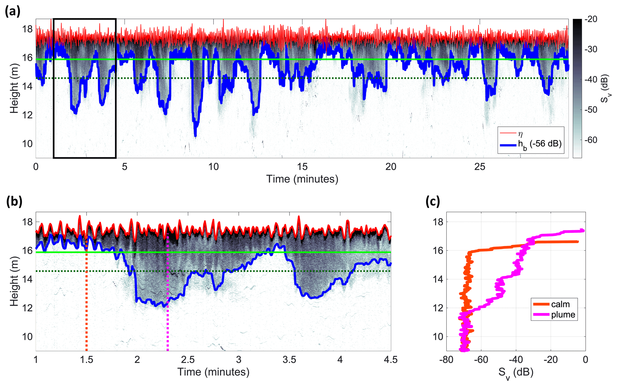
Figure 2 Example of measured air bubble plume echo. The wind speed U₁₀ was 8 m s⁻¹ and the significant wave height was H_s=1.3 m. (a) Time–height volumetric backscatter strength S_v (grey shading, units in dB). Backscatter height (in m) is measured upward from the sea bottom. Bubble plume height h_b (blue line; threshold level of −56 dB) and surface wave elevation η (red line). The solid light-green and dashed dark-green lines show the depth H_s and 2H_s, respectively. The solid black rectangle shows the echo chunk zoomed in (b). (b) Zoom of (a) between 1.0 and 4.5 min. (c) Vertical profiles (up to the air–sea interface) of backscatter strength during a calm period (dashed orange vertical transect in b) and within a bubble plume (dashed violet vertical transect in b).

In the example shown in Fig. 2a, bubble plumes display a growth phase, where air entrainment driven by downward forces is expected to dominate and the plume deepens to a peak depth which is followed by a decay phase, during which the bubble rise dominates. Individual deeper plumes are not symmetric around the lowest depth, and the growth time is generally smaller than the decay time. Two distinct layers where air bubbles can evolve are visible (Czerski et al., 2022). On the one hand, a shallow and near-permanent stratus layer of bubble persists from the surface to a depth qualitatively just below the significant wave height and responds naturally to the orbital motion of surface waves (see, e.g. the echo signal around 1.5 min in Fig. 2b). This layer is sustained by wave breaking and is advected by Stokes drift and wind-driven currents.

On the other hand, at deeper depths, separate bubble plumes are located in individual cells, often in close succession, and have a lifetime of roughly 30–120 s (far exceeding the period of their generation by wave-induced turbulence). The lifetime may also depend on the horizontal size of the plumes and the magnitude of the near-surface current. Thorpe (1986b) provided evidence of an increase in the bubble plumes with current and a decrease in their duration. Downward water advection may also occur at the convergent limb of Langmuir cells, which are thought to have a role in forming deep plumes (Czerski et al., 2022). Figure 2c compares the volumetric scatter strength profiles from the centre of a plume and a calm zone where no deep plume is detected. The calm zone displays scattering levels for ambient noise around −70 dB (consistent with Cifuentes-Lorenzen et al., 2023) close to the surface (height of 16 m), from where it rapidly increases up to a maximum level. The plume profile, conversely, shows a measurable scattering level starting from about 12 m from the seabed that intensifies towards the surface. The contrast in backscattering levels between the plume and the calm zone profiles reaches 40 dB.

3.2 Measurement of the bubble plume penetration depth

The volumetric backscatter signal S_v(t,h) is processed to identify the temporal evolution of the bubble plume's lower edge (from the air–sea interface). This procedure is possible since the scatter strength decreases within each bubble plume with increasing vertical distance from the water surface, with larger S_v levels in the uppermost metre. On the other hand, close to the seabed, the echo signal is dominated by the background noise. Therefore, the histogram of S_v is bimodal, with a distinct separation between the two echo environments. This behaviour permits us to determine bubble depth using a cut-off threshold approach, with empirical values normally ranging from −70 to −50 dB (Cifuentes-Lorenzen et al., 2023; Czerski et al., 2022; Derakhti et al., 2024; Gemmrich, 2010; Saetra et al., 2021; Strand et al., 2020; Thorpe, 1986b; Trevorrow, 2003; Vagle et al., 2010; Wang et al., 2016). Likewise, in this study, the depth of the bubble plume is identified with the method described below.

Firstly, the 2-D echogram S_v(t,h) is smoothed using a median filter with a size of [3×3], corresponding to 1.5 s in time and 7.5 cm in the vertical range. Then, on the smoothed echo, the bubble height (h_b) is measured upward from the seabed and is defined as the point where the backscattered signal goes above a threshold. The threshold is selected empirically as being not contaminated by the ambient noise (about −70 to −60 dB) and adapted for each S_v(t,h) to equal $min\mathit{\{}\underset{\mathrm{¯}}{S}+\mathrm{10}\mathrm{dB},-\mathrm{50}\mathrm{dB}\mathit{\}}$, where $\underset{\mathrm{¯}}{S}$ is the average scatter strength in the lowest third of the vertical range; this way, we account for the episodic increase in the ambient backscattering in the lowest part of the range due to fine-sediment resuspension from the seabed. In practice, the selected thresholds ranged between −56 and −50 dB. We point out that we set a constraint that the signal must be continuous along the selected threshold or else it is removed. In this manner, zones of less scatter surrounded by regions of above-threshold scatter can be retained. An example of the identified bubble height time series h_b(t) is shown in Fig. 2 (solid blue line).

The thickness of the bubble layer (the bubble depth, z_b) is measured as the vertical distance from the instantaneous sea surface elevation η (see next section for its determination) to the bubble height h_b, such that

$$\begin{array}{}\text{(6)}& z_{\mathrm{b}}\left(t\right)=\mathit{\eta }-h_{\mathrm{b}}.\end{array}$$

Remapping bubble profiles to wave-following coordinates reduces the aliasing effect due to the surface wave orbital motions in determining the bubble depth (Gemmrich, 2010; Trevorrow, 2003; Wang et al., 2016). From the time series of z_b, two quantities are considered later in this study: (i) the 30 min average (z_ba), which gauges as a whole the processes of injection, raising, and residing of bubbles in the water column; (ii) the 90th percentile (z_b90), which is a measure of the deeper depths reached by the plume. The timeline of these two depths is referenced to +15 min of each hour, and all auxiliary variables (see next section) are interpolated over the same axis.

In evaluating vertical-looking sonar measurements of bubble plumes, it is important to recognize some elements. While it would be desirable to identify the growth and decay phases of plume evolution, the lack of information on the surface whitecap evolution and the 2-D time–height nature of the sonar observations do not allow us to distinguish between growth and decay, since the latter can be further elongated in time by successive breaking. Therefore, as in previous studies, we consider the entire time series of bubble depth to infer the relationship with environmental forcings. Moreover, the horizontal scale of bubble plumes on the water surface exceeds the width of the sonar beam, which can detect only a 1-D vertical transect of what is eminently a 3-D phenomenon. Therefore, it is not possible to resolve the difference between bubble plumes that are locally produced and those which are advected through the vertical of the sonar beam (Czerski et al., 2022; Thorpe, 1982). In each echo record, spatial and temporal effects are not distinguished, and no information can be derived about the horizontal extent of the plume. This is the typical problem that is found in the study of 3-D ocean wave elevations from the analysis of temporal wave records (Ochi, 1998). As for waves, we assume the ergodicity of the bubble depth process, and statistical properties are evaluated from the analysis of a single record z_b(t).

3.3 Auxiliary observations and methods

The acoustic instrument can also measure the sea elevation time series η(t) by echo ranging to the surface with the vertically oriented transducer (altimeter). Operationally, the surface level is defined by applying a matched filter over a series of cells to locate the maximum return signal, which marks the well-distinct separation between water and air (red line in Fig. 2a, b). This operation is carried out by the instrument processor for each 30 min burst with no intervention by the user. The significant wave height H_s is computed as 4 times the standard deviation σ of η(t), i.e. H_s=4σ, and the wave variance frequency spectrum E(f) is estimated via discrete Fourier transform using the Welch estimator with standard settings. Furthermore, a thermistor (accuracy of 0.1 °C) embedded in the head monitored the water temperature at the same temporal rate as the sonar. Originally designed to adjust the speed of sound, the near-seabed water temperature is used in this study to inspect the presence of cold-water masses. The ADCP was also used to measure the vertical components of the water velocity at 2 Hz and a cell size of 0.5 m.

Sonar observations are complemented by measured atmosphere and sea data from Acqua Alta. These are used to characterize the environmental forcing and bulk air–sea fluxes. The horizontal mean wind speed U and direction were measured 23 m above sea level with an anemometer mounted on the Vantage Pro2™ weather station. The anemometer is attached to the Acqua Alta tower about 10 m above the structure to reduce its influence on observations. Data are averaged every 5 min (i.e. 12 values every hour), and the accuracy is 0.1 m s⁻¹ for the wind speed and 7° for wind direction. The same sensor provided the air temperature (accuracy of 0.5 °C). The near-surface water temperature was measured 3 m below the mean sea level by a Sea-Bird SBE 37-SMP-ODO pumped MicroCAT recorder.

To identify crossing wave conditions and isolate wind waves, the directional spectrum of the wave field was measured using an additional acoustic wave and current profiler (AWAC) deployed at Acqua Alta. Wave directions θ are based on the first pair of Fourier coefficients and are used to describe the mean direction at a given frequency. From these coefficients, the directional wave spectrum is expressed as a composition of the frequency spectrum E(f) and the directional distribution D(f,θ). From this, the partitioning of the wave systems (wind–sea and swell) was obtained with an automated procedure of the direction/frequency spectrum based on the watershed algorithm of Hasselmann et al. (1996), which treats the wave spectrum as an inverted catchment area, following the implementation of Hanson and Phillips (2001). The wind–sea partition was chosen as the one with peak direction in the same quadrant as the local wind; its significant wave height is indicated as H_s,ws.

Additional parameters that are relevant to air–sea interactions are computed using the COARE bulk algorithm (Fairall et al., 2011), version 3.6 (Fairall et al., 2022; https://downloads.psl.noaa.gov/BLO/Air-Sea/bulkalg/cor3_6/, last access: 29 April 2024). COARE includes the effect on fluxes of surface waves by considering in the surface drag formulation the significant wave height and phase speed of waves at the peak of the frequency spectrum. In this study, COARE is used to estimate, from measured values, the friction velocity in the air (u_∗), the actual wind at the reference 10 m height (U₁₀), the neutral stability wind at 10 m height (U_10n), and the total (sensible plus latent) heat flux across the air–sea interface (Q).

4 Results and discussion

The results presented in this section represent the principal characteristics of the bubble depth fields measured during the experimental campaign. We aim to inspect the surface forcings influencing the bubble penetration at the scale of sea states during different storms. Further, we compare our outcomes with those from experiments made in different sites and wind/wave conditions in search of consistency. This allows us to highlight the effect on the bubble plume scales and the deeper depths of the turbulence enhancement associated with the thermal instability of the water column. Results are discussed in the context of the theoretical predictions of the CO₂ transfer velocity (total and bubble mediated; see Appendix A) and its relationship with the penetration depth of bubbles.

4.1 Metocean conditions during two storms in the north Adriatic Sea

In this section, we describe the local conditions in the north Adriatic Sea for atmosphere and waves during two high-wind/wave events during which the bubble depth was measured by the sonar; specifically, the storms occurred on 8–9 December 2021 (storm S1) and 5–7 January 2022 (storm S2). Otherwise, during the experimental campaign, no other meaningful events were experienced (the wind speed remained below 7 m s⁻¹). Figure 3 sketches the model wind speed (from ECMWF ERA5 reanalysis) over the entire Adriatic Sea at two instants during the storms, whereas the observed time series of atmosphere and wave parameters are shown in Fig. 4. We anticipate that at Acqua Alta the two storms had similar values of total wave energy at the peak, with significant wave heights close to 3 m (in the region, storms with a significant wave height of 3 m at the peak have return periods of about 1 year; Benetazzo et al., 2022). In the north, where bubble plumes were observed, the characteristics of the two sea states were different, with S1 being composed of a mixed sea (swell from southeast superimposed to a turning wind–sea from east to northeast), while S2 experienced only wind-forced waves from northeast. As we shall see later, the different sea states led to a different short-term response of the bubble plumes.

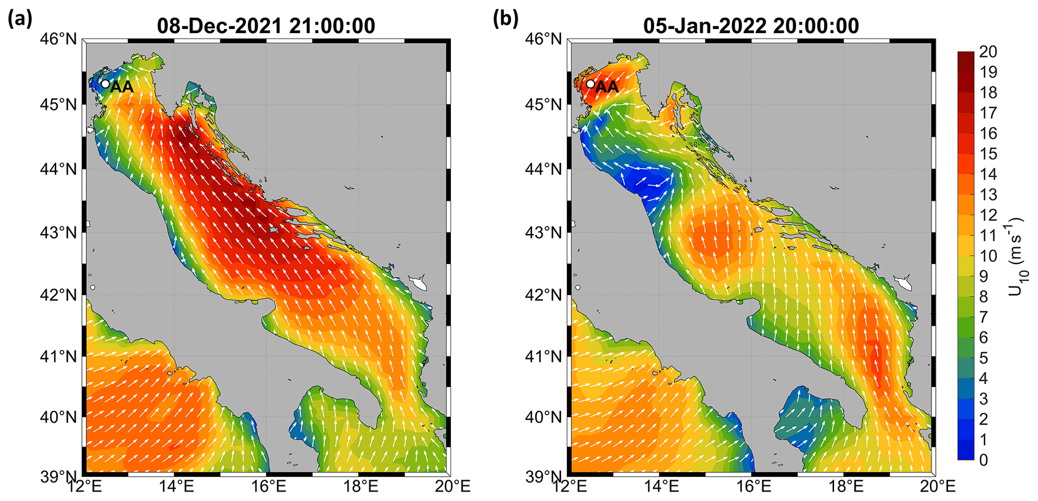
Figure 3 Adriatic Sea 10 m height wind speed (U₁₀, in m s⁻¹) and direction (white arrows) during two instants of storms S1 (a) and S2 (b). The AA label shows the position of the Acqua Alta oceanographic research tower. Numerical model data from ECMWF ERA5 reanalysis (https://cds.climate.copernicus.eu/cdsapp#!/dataset/reanalysis-era5-single-levels?tab=overview, last access: 29 April 2024; Hersbach et al., 2023).

Regarding storm S1 (Fig. 4a), the wind speed U₁₀ and direction (not shown) changed frequently on 8 December 2021 in the north Adriatic Sea. An alternation of northeasterly and southeasterly (from 11:30 to 14:00 and from 17:30 to 19:00 UTC) was observed (wind direction changes in panel (a) are indicated with vertical dashed black lines). The wind speed peak of 14.8 m s⁻¹ at 11:00 UTC on 8 December was reached during a northeasterly phase. Following the wind, the mean wave direction was from the northeast (63° N, on average) until 8 December at 12:00 UTC; then, it turned from southeast (135° N, on average) during the remaining part of the storm controlled by a large-scale circulation forcing southeasterly winds in the mid and south Adriatic (Fig. 3a). The series of significant wave height H_s accompanied the growth and drop of wind and peaked at 3.1 m on 8 December at 21:30 UTC. Since then, a steady reduction in the sea-state severity followed. Figure 5 shows the frequency energy spectrum E(f) and the directional distribution D(f,θ) of the wave energy at the storm's peak when the sea state was a combination of wind–sea and swell. The swell from the southeast had a peak frequency of 0.12 Hz, whereas less energetic wind waves from the northeast were concentrated around 0.23 Hz. The direction of the local wind was used to isolate the wind–sea part of the significant wave height to be included in the gas transfer parametrizations.

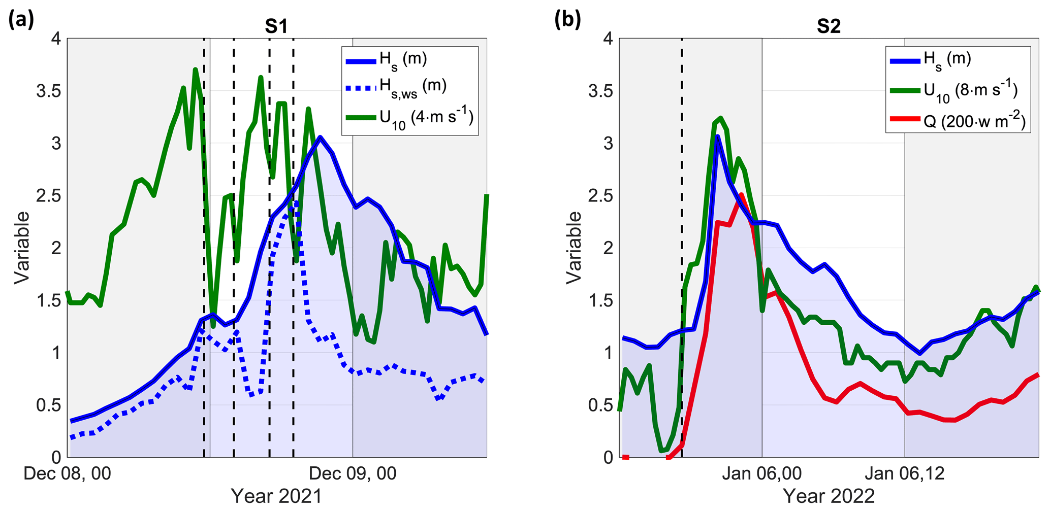
Figure 4 Atmosphere and wave conditions measured at the observation site. Variables: 10 m height average wind speed U₁₀ (in m s⁻¹), total significant wave height H_s (in m), wind–sea significant wave height H_s,ws (in m), and heat flux Q (in W m⁻²). Wind speed and heat flux are linearly scaled for graphical purposes with the coefficients provided in the legend. The vertical dashed black lines show the instant when the wind turned (see main text for a detailed description). (a) Mixed-sea storm on 8–9 December 2021. (b) Unimodal, cold-air storm on 5–6 January 2022.

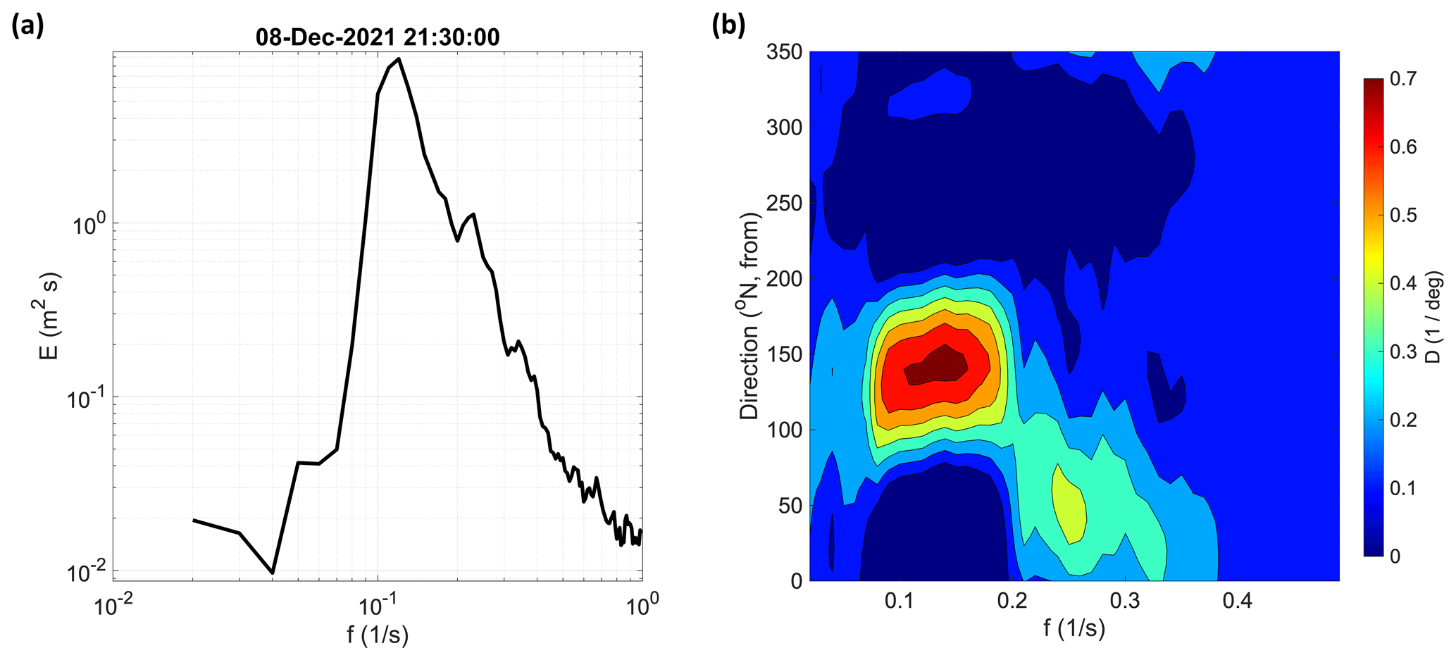
Figure 5 Wave energy distribution measured in the north Adriatic Sea on 8 December 2022 at 21:30 UTC (storm S1). (a) Wave-frequency spectrum E(f) and (b) directional distribution D(f,θ) of the wave energy.

Storm S2 (Figs. 3b and 4b) was initiated by a weak southwesterly on 5 January 2022, which suddenly turned from the northeast (the incoming mean direction was 36° N), bringing cold and dry bora wind in the north Adriatic Sea from 17:30 UTC. The wind speed U₁₀ reached 26 m s⁻¹ on 5 January at 20:30 UTC. The wave spectrum was unimodal, and H_s peaked at 3.1 m on 5 January at 20:00 UTC. The atmospheric condition was the one typical of a cold-air outbreak event (Vilibić and Supić, 2005): in 10 h, from 17:00 to 23:00 UTC on 5 January, the air temperature dropped by more than 8 °C, from 11.1 to 2.6 °C. The air–water temperature difference decreased to a minimum $\mathrm{\Delta }T=-\mathrm{7.3}$ °C at 23:00 UTC. The combination of gale-force wind and a large temperature difference between the water and air led to surface heat flux Q reaching 510 W m⁻² at the same time. For reference, during the 2012 record-breaking cold-air outbreak that partially iced the Venice lagoon, the heat flux at Acqua Alta reached 800 W m⁻² (Benetazzo et al., 2014). During S2, the sign of thermal vertical convection was recorded by the thermometer near the seabed. On 5 January 2022, in 30 min, from 20:00 to 20:30 UTC, the water temperature decreased from 11.2 to 10.3 °C. Near the seabed, the minimum recorded temperature during S2 was 10.0 °C, and after the storm it stabilized at around 10.3–10.5 °C, about 1 °C colder than before.

4.2 Response and scales of the bubble plume

With the method described earlier, the 30 min time series of bubble depth z_b was measured at 1 h intervals. We focus on the two storms, S1 and S2, highlighting the principal characteristics of the average (z_ba) and 90th percentile (z_b90) bubble depth. The results are shown in Fig. 6.

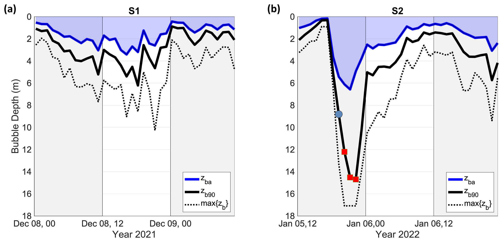
Figure 6 Time development of the bubble plume depth z_b during the S1 (a) and S2 (b) storms. Values of the average (z_ba; solid blue line) and 90th percentile (z_b90; solid black line) of the bubble depth. The dotted black line shows the maximum bubble depth max{z_b}. In (b), the red markers show instants on the z_b90 curve when the bubble plume reached the sonar head, and the blue–silver marker shows the instant of the sonar record in Fig. 7, which was taken at the onset of the cold-air outbreak.

During storm S1 (Fig. 6a), the average depth z_ba responded at a short time scale to the change in wind speed and direction and exceeded 3 m (3.4 m, at most) during the two phases of northeasterly wind when the wind speed was as high as 14 m s⁻¹. The series of z_b90 follows closely that of z_ba (the correlation coefficient (CC) between the two data sets is 0.99), and the extreme to average depth ratio $\mathit{\gamma }=z_{\text{b90}}/z_{\text{ba}}$ was, on average, equal to 1.8. This ratio is slightly smaller than that found by Strand et al. (2020), who used, however, the maximum value of z_b as a numerator in γ. We have also found a very high correlation (CC=0.90) between z_ba and wind speed U₁₀ and a very poor correlation (CC=0.15) between z_ba and total H_s. The latter is due to the rapid changes in the wind direction that continuously led to non-equilibrium conditions for wave input and dissipation. Indeed, rotating winds made the energetic wave components close to the spectrum's peak largely angled from the wind, thereby receiving a small momentum. Considering only the wind–sea part of the wave spectrum, the correlation coefficient between H_s,ws and z_ba increases to 0.47, which is still smaller than values found in previous studies. During the most intense phases of the storm, the maximum z_b, max{z_b}, was above 6 m and peaked at 10.3 m.

The vertical scales of the bubble plume were different during storm S2 (Fig. 6b), which was characterized by steady wind–sea conditions from 5 January 2022 at 17:30 UTC onwards. The average value of the bubble depth reached 6.6 m, and the correlation of z_ba was high with both U₁₀ (CC=0.95) and H_s (CC=0.84), in line with values obtained by Strand et al. (2020). Remarkably, the ratio γ reached 3 across the peak of the heat flux (from 20:00 to 23:00 UTC on 5 January), when the deepest portion of the bubble plume extended to the sonar head close to the seabed (about 17 m deep). At that time, z_b90 reached 6.1H_s. Afterwards, on the storm's decay, the ratio $z_{\text{b90}}/z_{\text{ba}}$ decreased and was, on average, equal to 2.1, in line with values found during S1.

The backscatter of the bubble plume at the onset of the cold-air outbreak is shown in Fig. 7a. It represents a period (starting on 5 January 2022 at 19:00 UTC, denoted by a blue–silver marker in Fig. 6b) when a medium-severity sea state (H_s=1.7 m) was suddenly forced by a strong and cold wind (U₁₀=21.5 m s⁻¹, $\mathrm{\Delta }T=-\mathrm{3.4}$ °C) which produced individual deep bubble plumes easily distinguishable from the background bubble population. The maximum thickness of the bubble depth reached 13 m (about 8H_s), and z_b90 reached 8.8 m. There is a notable trend of bubble plume deepening with time, which we estimate has a rate of about 12 m h⁻¹. Figure 7b shows the vertical component (w) of the water velocity after low-pass filtering the raw signal at 0.10 Hz to remove the contribution of the wave orbital motion (the peak of the wave frequency spectrum was at 0.16 Hz). This way, the vertical convection in the mixing layer is considered; we note that negative velocities (i.e. downward) around −7 cm s⁻¹ accompany the creation of deeper plumes. This speed value is consistent with the prediction by Thorpe (1982), who estimated the maximum depth to which bubbles are carried as a function of the downward water current to be $max\mathit{\left\{}{z}_{\mathrm{b}}\mathit{\right\}}=\mathrm{1.9}w=\mathrm{13.3}$ m (with z_b in m and w in cm s⁻¹). We note that stronger echo intensities are located in regions with larger vertical speeds, probably indicating locally generated plumes.

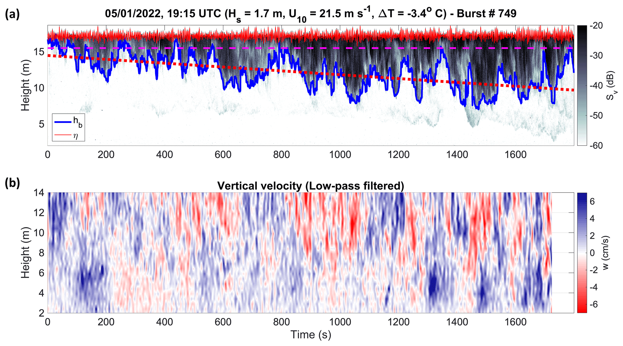
Figure 7 Response of the air bubble plume at the onset of the cold-air outbreak on 5 January 2022. (a) Volumetric backscatter strength S_v is in grey shading (in dB). Backscatter height (in m) is measured upward from the sea-bottom level. The bubble plume height is shown with a blue line and the surface wave elevation η with a solid red line. The dashed magenta line shows the depth of H_s, and the dotted red line shows the line of best fit of the bubble depth. (b) The vertical component w of the residual velocity (in cm s⁻¹; positive upward) after low-pass filtering w at 0.1 Hz.

Different stages of storm development led to bubble plume shapes that can be characterized and compared with wave characteristics. In this respect, the frequency spectra E(f) of surface wave elevation and bubble height are shown in Fig. 8. Data are plotted for storm S2 and correspond at instants before the peak of the storm (panel a), at the onset of the cold-air outbreak (panel b), and after the peak of the storm (panel c). Two different behaviours can be observed for the bubble height. For the first type (panels a and c), we found that wind waves near the peak of the wave-frequency spectrum produce breakers and displace newly produced or resident bubbles in the water body; in this case, wave elevation and bubble height spectra have similar energy levels above about half the peak frequency and, over it, spectra follow an f⁻⁴ law, in agreement with wave theory (Zakharov and Filonenko, 1967). Unlike waves, long-period, slow, and coherent motions dominate the bubble height energy in all conditions. These motions have characteristic periods of at least about 3 times the period of the dominant wave components that are closely linked with the wave-breaking periodicity (Malila et al., 2022). This finding aligns with the results reported in Derakhti et al. (2024). For the second type of behaviour (panel b), in conditions where the vertical motion of the water bulk is also driven by thermal convection, surface-wave and air-bubble temporal scales are partially decoupled. Whereas the former preserves the typical spectral shape (peak followed by a tail), the latter shows a continuous spectrum over the frequency range (no peak is evident), which decays with a milder shape proportional to f⁻².

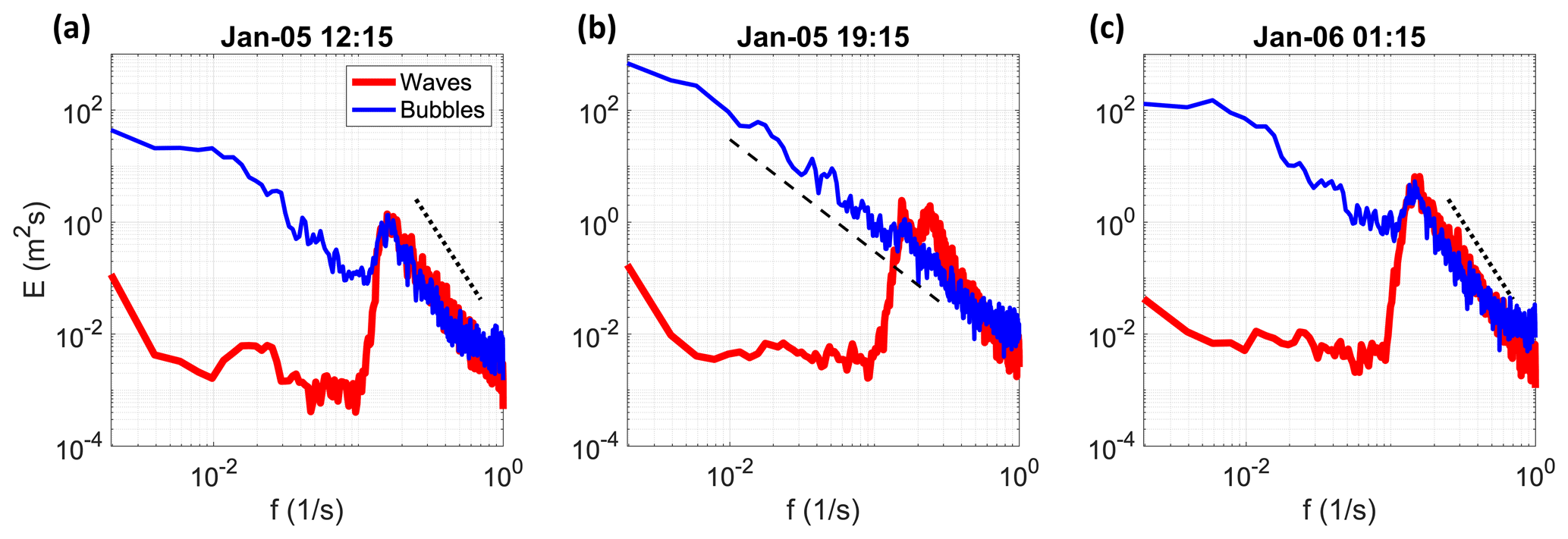
Figure 8 Frequency spectra (E, in logarithmic scale) of wave elevation and bubble height at different stages of storm S2. (a) The record before the storm peak (on 5 January at 12:15 UTC), (b) at the onset of the thermal convection (on 5 January at 19:15 UTC), and (c) after the storm peak (on 6 January at 01:15 UTC). A dashed black line shows the slopes of f⁻⁴ (a, c) and f⁻² (b).

During storm S2, for the hours when the thermal convection was not relevant, the wave elevation η and bubble depth z_b histograms are shown in Fig. 9a. Waves follow a normal distribution closely, but data are positively skewed (the skewness coefficient is, on average, 0.14). On the other hand, bubble depths are distributed around a lognormal distribution, as already found by Strand et al. (2020). Lognormality may suggest that the bulk of depths reached by bubbles is determined as the product of a set of independent forces at play simultaneously. Although vertical-looking sonar data do not enable clear discrimination of all factors, the temporal and spatial evolutions of entrained bubbles arise from a combination of turbulence and advection associated with breaking waves and Langmuir circulation, buoyancy of bubbles, and bubble growth or shrinking (hydrostatic pressure and net exchange of all gases). The lifetime of the bubble plume depth z_b is shown in Fig. 9b during S1 and S2 (excluding data from the cold-air outbreak). The two lifetime distributions show similar exponential decay with increased depth. During S2, the average z_b is 1.04H_s, close to the penetration depth considered in the bubble-mediated gas transfer model by Deike and Melville (2018). We observed a population of bubbles that get deeper than H_s: bubbles at depths above 2H_s have a modest lifetime (14 %), and at depths above 4H_s they are rare.

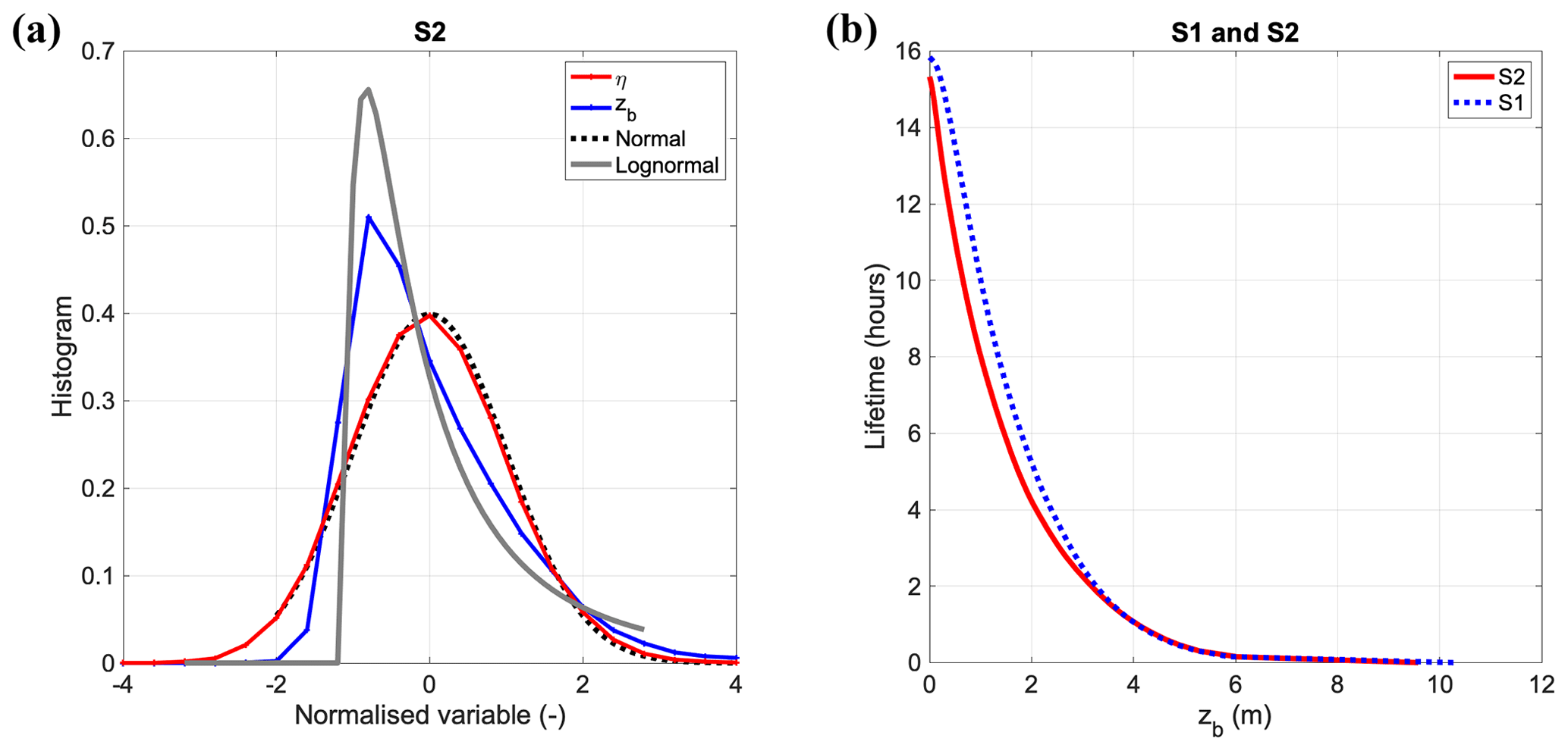
Figure 9 Distribution of bubble plume penetration depth. (a) Histogram of normalized (zero mean and unitary standard deviation) wave elevations η and bubble depths z_b during storm S2. Normal (dashed grey) and lognormal (solid grey) distributions are plotted for comparison. (b) The lifetime of the bubble plume depth z_b during S1 (all data) and S2 (excluding data during the cold-air outbreak).

4.3 Bubble depth and surface forcings

We consider here the observations of bubble depth and the relationship with wind speed and a combination of wind and waves. At first, bubble data are interpreted using a linear law with U₁₀ to compare the observed depths with predictions from parametrizations (Fig. 10a). This way, the strength of breaking and any other phenomena governing the deepening and rising of bubbles are largely simplified. The average bubble plume depth z_ba (in m) is written as a function of U₁₀ (in m s⁻¹), and experimental data are fitted with a linear relationship in the following form:

$$\begin{array}{}\text{(7)}& z_{\text{ba}}=\mathit{\alpha }(U_{\mathrm{10}}-U_{\text{min}}),\end{array}$$

which ensures that as the forcing term approaches a minimum threshold U_min, z_ba approaches 0, which is what is physically expected. The scaling coefficient α (in s) indicates the effectiveness of the forcing process (wind) to displace bubble plumes under the water surface; α is estimated as 0.33 and 0.31 during S1 and S2, respectively, while the onset of detectable bubbles is at a speed U_min of 3.3 and 3.2 m s⁻¹, respectively. This minimum wind speed for having detectable bubbles is consistent with that found in previous studies on bubble and whitecap production (Hanson and Phillips, 1999; Monahan and O'Muircheartaigh, 1986). Despite the significant variability in wind direction and speed experienced during S1, we find a good fit, i.e. R²=0.86. The quality of predictions improves for S2 (R²=0.91). The law governing the average bubble depth with wind speed shows little difference between storms despite the great variability of wave conditions (mixed sea during S1 and unimodal during S2). Moreover, there is no clear evidence of thermal convection effects on z_ba during S2. In fact, we observed that the average bubble depth adapts rapidly to wind conditions and is mainly influenced by the almost continuous stratus layer of bubbles below the surface. More than U₁₀, surface processes are captured by the friction velocity u_∗, whose relationship with z_ba is shown in Fig. 10b. A linear law approximates well the data scatter, and the minimum friction velocity for having detectable bubbles is, on average, 5.5 cm s⁻¹.

For a given wind speed U₁₀, bubble depths measured here are smaller than those found in previous research, which parametrized the mean bubble depth with a similar law (Eqs. 1–4). For the purpose of the present study, the Strand et al. (2020) measurements of z_ba versus U₁₀ have been fitted with a linear law to reconcile with previous parametrizations. The law obtained is as follows (with ±95 % confidence bounds):

$$\begin{array}{}\text{(8)}& z_{\text{ba}}=\mathrm{0.53}\pm \mathrm{0.01}(U_{\mathrm{10}}-\mathrm{1.6}\pm \mathrm{0.1}),\end{array}$$

with a coefficient of determination R²=0.72.

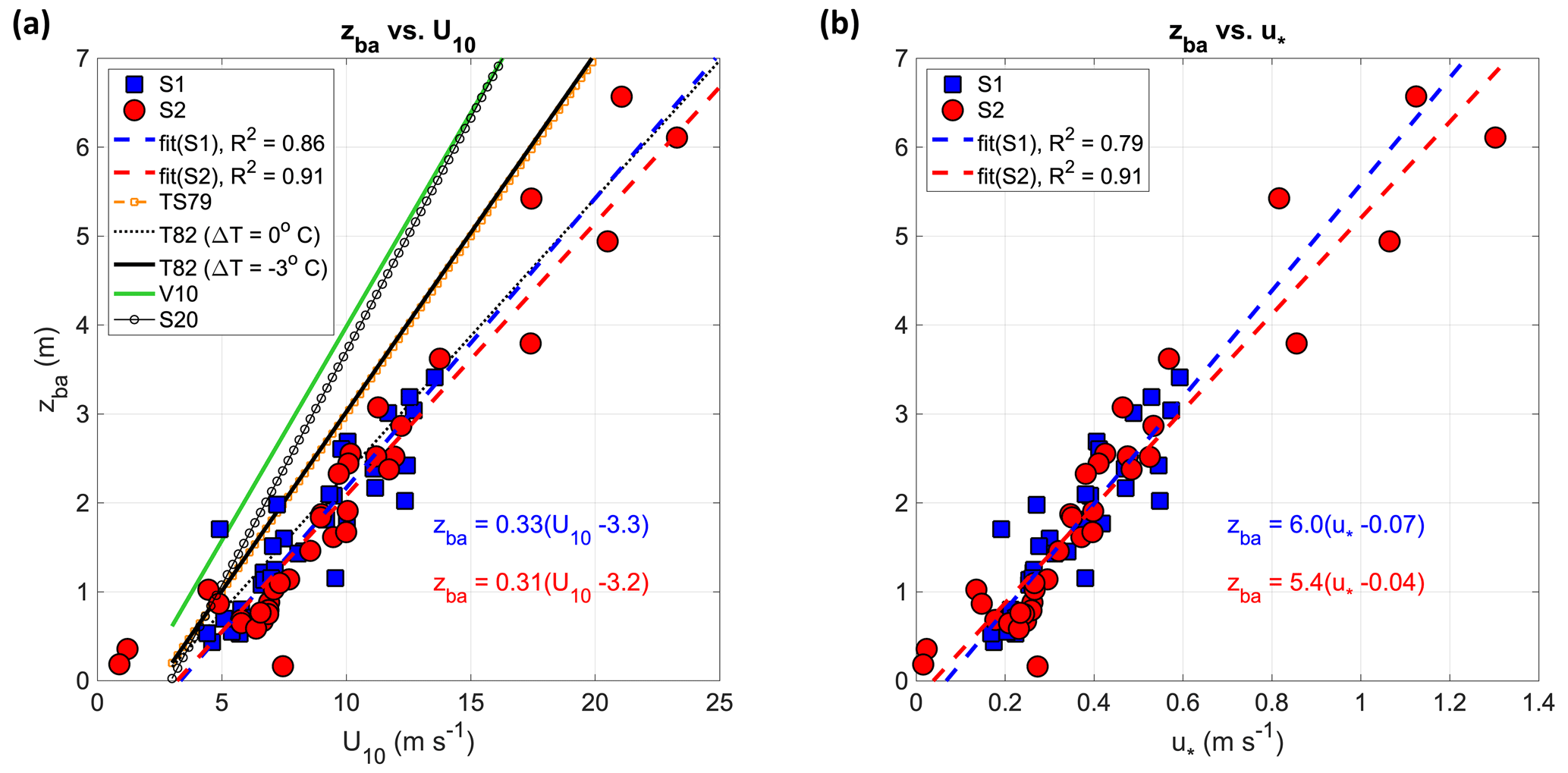
Figure 10 Relationship between bubble plume depth and wind parameters. Average bubble penetration depth z_ba versus 10 m height wind speed U₁₀ (a) and friction velocity u_∗ (b). Empirical data over storms S1 (blue marker) and S2 (red marker) and lines of best fit (dashed curve; equations in the plot area with the same colour code). Reference curves: TS79 (marked orange line), Thorpe and Stubbs (1979); T82 (ΔT=0 °C) (dotted black line), Thorpe (1982) with air–water temperature difference ΔT=0 °C; T82 ($\mathrm{\Delta }T=-\mathrm{3}$ °C) (solid black line), Thorpe (1982) with air–water temperature difference $\mathrm{\Delta }T=-\mathrm{3}$ °C (the mean temperature difference during storm S2); V10 (green line), Vagle et al. (2010); S20 (marked black line), a fit of Strand et al. (2020) data.

Compared to the data presented in this study, only the relationship by Thorpe (1982) setting the air–water temperature difference to 0 (ΔT=0 °C) tends to agree. This discrepancy suggests that existing parametrizations of bubble depth versus wind speed implicitly incorporate in coefficient α the wave characteristics used during the experiments as the basis of the investigation. This indicates that the wind speed alone cannot parametrize bubble depths in all conditions, as also pointed out by Cifuentes-Lorenzen et al. (2023). In comparing the data presented here with others of similar characteristics, one must also note that bubble depths can depend on the sonar frequencies and echo thresholds (Czerski et al., 2022). This effect is, however, not straightforward to quantify, and we assume it is of second-order influence compared to the effect of environmental forcings generating bubble plumes.

An effective way for including wave effects in the forcing process is given by equally weighting sea-state severity (say H_s) and wind friction velocity through the wind/wave Reynolds number R_H given by (Zhao and Toba, 2001)

$$\begin{array}{}\text{(9)}& R_{\mathrm{H}}={\displaystyle \frac{u_{\ast }{H}_{\mathrm{s}}}{{\mathit{\nu }}_{\mathrm{w}}}},\end{array}$$

where ν_w is the kinematic viscosity of water. In a fully developed sea, the product u_∗H_s of water-surface processes is near-cubic with the wind speed, suggesting that wave energy dissipation plays an important role. This implies that for a given wind speed, the effect can be greater for a more developed sea (large H_s). Here we parametrize z_ba in terms of the whitecap coverage f_w, for which we used the formula proposed by Brumer et al. (2017b) that incorporates in the f_w estimate a measure of the wave severity (the significant wave height) in the following form:

$$\begin{array}{}\text{(10)}& f_{\mathrm{w}}=\mathrm{5.38}\times {\mathrm{10}}^{-\mathrm{6}}{R}_{\text{H}}^{\mathrm{0.88}}.\end{array}$$

The scatter between z_ba and f_w is shown in Fig. 11. A power law fit for S2 data (dashed red line) provides good accuracy (R²=0.87), with data having a high correlation (CC=0.92). The shape of the power law suggests that z_ba scales closely to $\sqrt{u_{\ast }{H}_{\mathrm{s}}}$. This indicates that the coefficient α in Eq. (7) is not constant with wind speed but is such that α=α (wind speed, H_s). We note that other parameters, like the wave steepness, can also be relevant for determining the bubble plume depths (Derakhti et al., 2024). Extrapolating, the threshold of f_w over which bubbles are detectable is 0.05 %. Formulating the plume depth z_ba via R_H tends to reconcile different data sets of bubble plume depth (Fig. 11), like those by Strand et al. (2020) and by Vagle et al. (2010); for the latter, we have estimated the significant wave height (not available in that study) using the Pierson–Moskowitz spectrum assuming fully developed sea states (Pierson and Moskowitz, 1964). A direct comparison between measured bubble plume depths and whitecap coverage is provided by Derakhti et al. (2024), who noted that bubble plume depths tend to increase with increasing whitecap coverage but at a lower rate (the exponent in the fitting is less than 1).

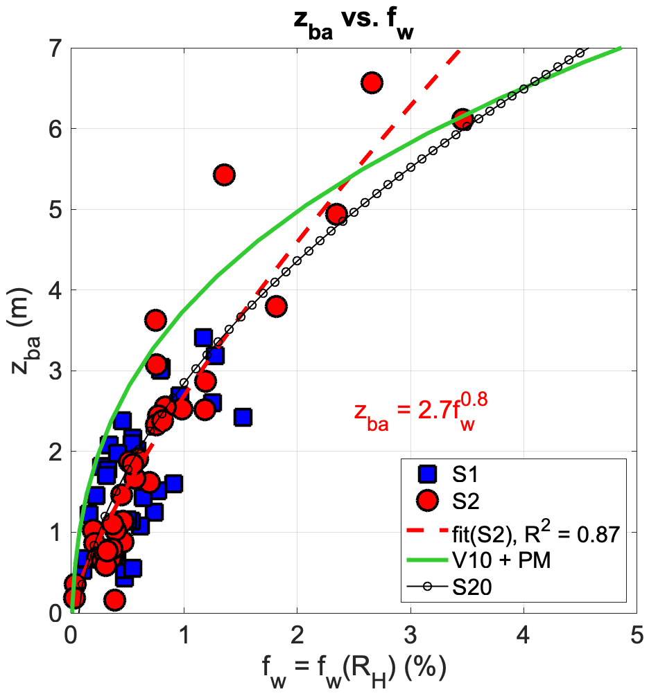
Figure 11 Relationship between (measured) average bubble plume depth z_ba and (theoretical) whitecap coverage f_w estimated after Brumer et al. (2107b) using the wind/wave Reynolds number R_H; data for storms S1 (blue marker) and S2 (red marker) and curve of best fit for S2 (dashed red curve; the equation is given in the plot area). The solid green line depicts Vagle et al. (2010) data (V10) complemented by the significant wave height estimated from the wind speed using the Pierson–Moskowitz (PM) spectrum. Strand et al. (2020) bubble data (S20) are shown with a marked black line.

The relevance of the bubble influx from the deeper plume events is conveyed by z_b90, the scatter of which against U₁₀ is shown in Fig. 12. As for z_ba, values of z_b90 closely follow a linear dependence on the wind speed across both storms; accordingly, the relationship against U₁₀ can be parametrized using the same law as in Eq. (7). For storm S2, we have not considered, in the fitting, values of wind speed when the heat flux Q>400 W m⁻², characterizing the hours around the peak of the cold-air outbreak (colour-mapped markers and black arrow lines). For the remaining points, we find a similar behaviour during storm S1, $z_{\text{b90}}=\mathrm{0.46}(U_{\mathrm{10}}-\mathrm{2.2})$, with R²=0.77, and storm S2, $z_{\text{b90}}=\mathrm{0.46}(U_{\mathrm{10}}-\mathrm{2.0})$, with R²=0.79.

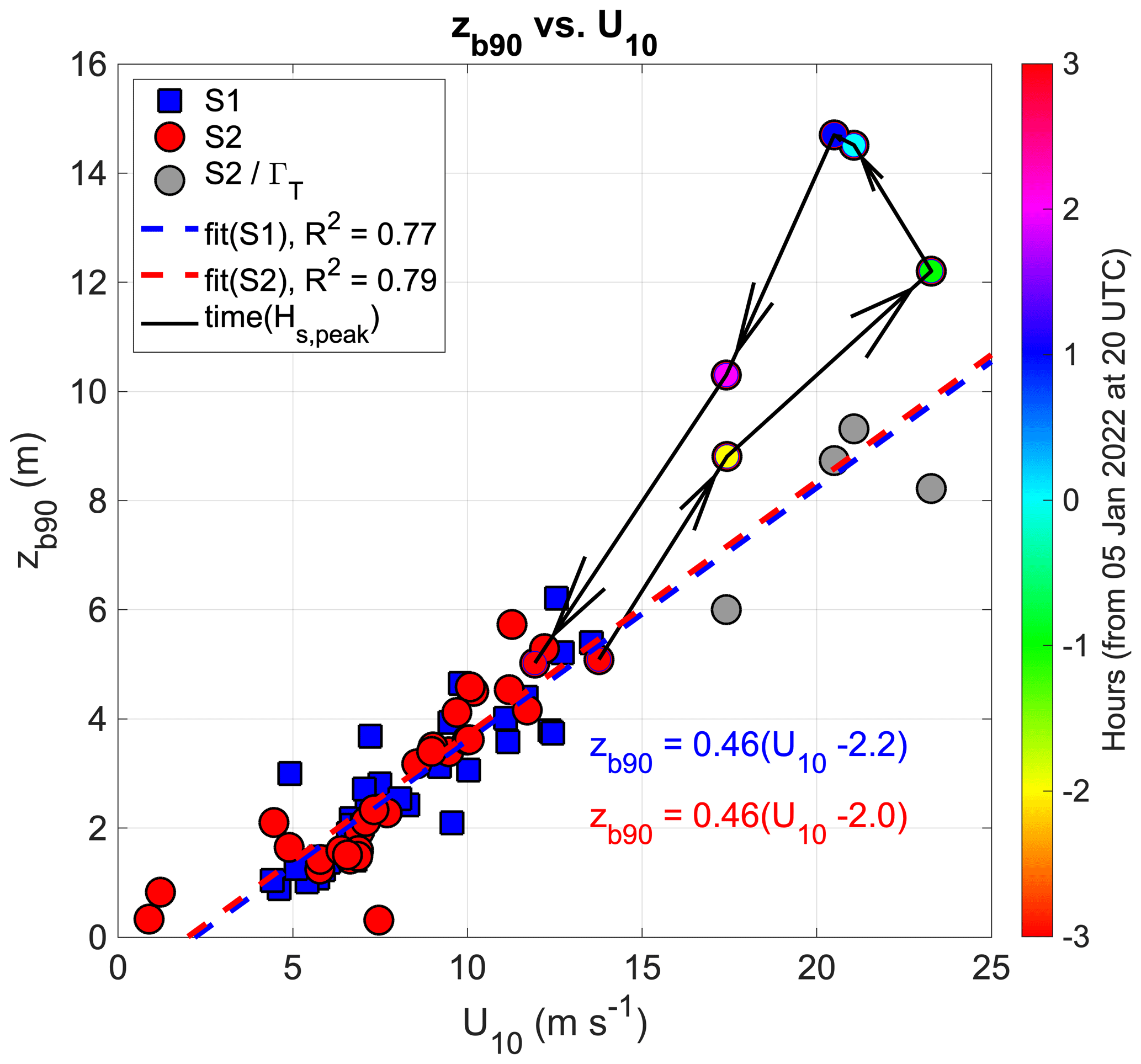
Figure 12 Relationship between 90th percentile of the bubble depth z_b90 and 10 m height wind speed U₁₀. Empirical data from storms S1 (blue marker) and S2 (red marker) and lines of best fit (dashed curve; equations in the plot area with the same colour code). Colour-mapped markers and black arrow lines indicate values during S2 from −3 to +3 h across the peak of heat flux Q. Grey markers show the same points but corrected (z_b90,corr) with the stability parameter Γ_T.

The impact of the sinking of the water masses during the cold-air event produced extreme depths z_b90 that were, on average, larger than those predicted in stable conditions of the water column. Correcting the measured z_b90 for the water-column stability parameter Γ_T in the following form

$$\begin{array}{}\text{(11)}& z_{\text{b90,corr}}=z_{\text{b90}}/{\mathrm{\Gamma }}_T,\end{array}$$

we find that the depth versus U₁₀ distribution agrees better with those from the other storm phases (grey circle markers in Fig. 12). Further, by following the temporal evolution of z_b90 across the peak of H_s, we observe values of up to +40 % during the set-down period of the storm (2–3 h after the peak) than during its intensification (3–2 h before the peak). Larger depths were reached when the air–water temperature difference ΔT was the lowest. If proportionality is anticipated between bubble penetration depth and gas transfer velocity, this evolution across the storm peak reverses the hysteresis cycle for the bubble-mediated CO₂ gas transfer velocity k described by Deike (2022). Indeed, not including the stability of the water column but only wind and wave parameters in forcing gas transfer, Deike (2022) found values of k up to a factor of 2 higher during the storm intensification period than during the set-down of the same storm.

4.4 Bubble depth and CO₂ transfer velocity

In this section, we explore the link between the observed bubble plume depths and the theoretical estimates of the air–sea transfer velocity of CO₂. The latter is determined using the forcing data measured during the two storms. Our goal is to evaluate the similarity of the relationship between external forcings, e.g. wind and waves, and their effect on bubble penetration and gas transfer velocity. This may also suggest a means of improving the current parametrizations used to predict the plume depths and transfer velocity of CO₂.

The air–sea exchange of CO₂ is generally calculated using a law that relates gas flux F with transfer velocity k and gas concentrations in the bulk liquid C_w and at the top of the liquid boundary layer adjacent to the atmosphere C₀, as follows (Keeling, 1993; Wanninkhof et al., 2009; Woolf, 1997):

$$\begin{array}{}\text{(12)}& F=k(C_{\mathrm{w}}-C_{\mathrm{0}}).\end{array}$$

By convention, F is negative for a gas flux from the atmosphere to the sea. To compare variations in diffusivity, the CO₂ transfer velocity is also given relative to the seawater-temperature-dependent Schmidt number Sc=660 (the value of Sc for CO₂ in seawater at 20 °C) as follows (Wanninkhof, 2014):

$$\begin{array}{}\text{(13)}& k_{\mathrm{660}}=k{\left({\displaystyle \frac{\mathit{Sc}}{\mathrm{660}}}\right)}^{\mathrm{1}/\mathrm{2}}.\end{array}$$

The kinematic parameter k represents the gas mass transfer resistances of various physical forcing mechanisms. It incorporates the dependence of the transfer on the diffusivity of the specific gas in water. The transfer can be effective directly across the sea surface or between a bubble (that encapsulates part of the atmosphere) and the water surrounding it for poorly soluble gases in rough sea conditions. The bubble-mediated flux is most effective when bubbles reside longer and deeper in the water volume, i.e. in stormy conditions. Since the efficiency of the bubble-mediated mechanism depends on the pressure within bubbles, which increases with depth, a correlation is expected to exist between gas exchange and the depth of the bubble plume.

The different processes involved in the exchange led to determining the total transfer as the sum of diffusive and bubble-mediated contributions (Woolf, 1997). To calculate total and individual contributions in turbulent water, two groups of parametrizations of k exist in the literature (see Appendix A and Table 1 for an overview of the formulations adopted in the present study). The first group assumes wind speed as the only kinetic forcing in the estimate, and here we consider the formula of the total k by Wanninkhof (2014; W14, from now on). The second group considers a combination of wind and waves, and we shall use for comparison the two formulae of the total k by Brumer et al. (2017a; B17, from now on), who differentiate between the total H_s and the wind–sea (subscript “ws”) H_s,ws, and by Deike and Melville (2018; DM18, from now on), and the two formulae of the bubble-mediated contribution to k (subscript “b”) by Woolf (1997; W97, from now on) and by DM18. Before going into the details of the principal outcomes, we note that coefficients in transfer velocity parametrizations should be adjusted to obtain a consistent mean value (Reichl and Deike, 2020). This calibration is not feasible in the present study because of the local nature and the short term of the experiment. The general behaviour, however, is preserved, and with this caveat in mind, the results are presented below.

Table 1 Formulations adopted in this study for the estimates of the air–sea transfer velocity k of CO₂ gas. Physical variables used as surface forcings: U_10n is the neutral stability wind speed at 10 m height, u_∗ is the friction velocity in the air, H_s is the significant wave height of the sea state, H_s,ws is the significant wave height of wind–wave partition of the sea state, and f_w is the whitecap fraction.

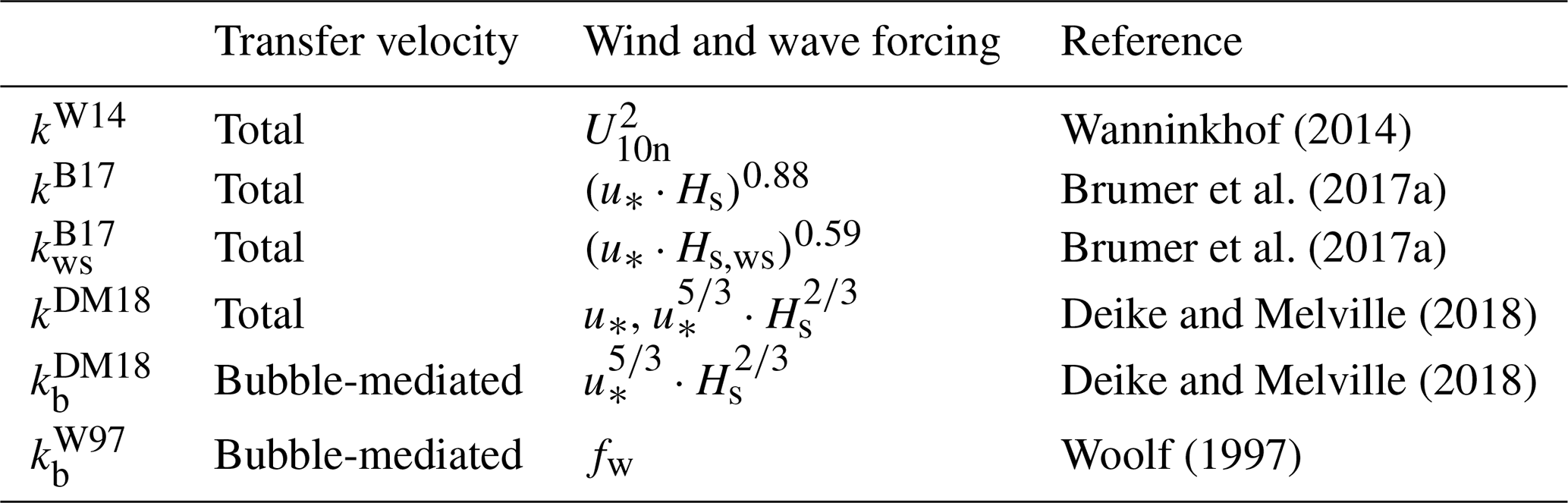
Figure 13 shows the time history, during storms S1 (panel a) and S2 (panel b), of total transfer velocities k^W14, k^B17, $k_{\text{ws}}^{\text{B17}}$, and k^DM18 and bubble-mediated transfer velocities $k_{\mathrm{b}}^{\text{DM18}}$ and $k_{\mathrm{b}}^{\text{W97}}$. As a consequence of the forcings used in the analysis, there is a remarkable difference between the two storms, such that transfer velocities from all parametrizations are approximately twice as large during S2 as during S1. Moreover, differences exist among individual estimates of k within each storm.

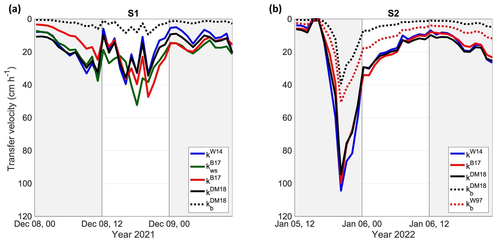
Figure 13 Time history of gas transfer velocity of CO₂ during storms S1 (a) and S2 (b). Theoretical estimates of the total velocity k according to parametrizations by W14 (k^W14, solid blue line), B17 (k^B17 and $k_{\text{ws}}^{\text{B17}}$, solid red and solid green lines, respectively), and DM18 (k^DM18, solid black line). Theoretical estimates of the bubble-mediated contribution to k according to parametrizations by DM18 ($k_{\mathrm{b}}^{\text{DM18}}$, dotted black line) and W97 ($k_{\mathrm{b}}^{\text{W97}}$, dotted red line).

During S1, k^W14 is smaller than 40 cm h⁻¹ and is consistent with k^DM18 (CC=0.99 and the absolute difference is 1.5 cm h⁻¹), whereas the transfer velocity $k_{\text{ws}}^{\text{B17}}$ produces higher values that reach 50 cm h⁻¹ during the most intense phase of the storm. Values of k^B17 correlate well with k^W14 and k^DM18 but display different behaviour during the growth and decay phases of the storm. The bubble-mediated contribution $k_{\mathrm{b}}^{\text{DM18}}$ is below 10 cm h⁻¹ due to a relatively small wind friction and dephasing between the wind speed peaks and wave severity. During S2, the three parametrizations of the total transfer velocity k^W14, k^B17, and k^DM18 provide similar values that peak around 100 cm h⁻¹; however, k^DM18 is smaller than k^W14 (−10 cm h⁻¹ at the peak), conveying the fetch limitations of the observed sea states, whose effect is included in DM18. The bubble-mediated term $k_{\mathrm{b}}^{\text{DM18}}$ is at most 40 cm h⁻¹, slightly smaller than $k_{\mathrm{b}}^{\text{W97}}$. The ratio of the bubble contribution to the total gas transfer velocity, according to DM18, reaches 27 % and 42 % during S1 and S2, respectively, in line with estimates from previous studies (Deike and Melville, 2018; Reichl and Deike, 2020).

The quadratic relationship between the total gas transfer velocity and wind speed adopted by W14 assumes that the wind primarily induces turbulence and shear in the ocean boundary layer. Turbulence fluctuations can be documented by the movement of small air bubbles, whose depths are large when fluctuations are also large. We then expect that proportionality exists between the bubble plume depths that we measured and the gas transfer, the link being the external forcing common to both processes. Based on this consideration, we investigate the relationship between bubble plume depths and $k_{\mathrm{660}}^{\text{W14}}$. The result is shown in Fig. 14.

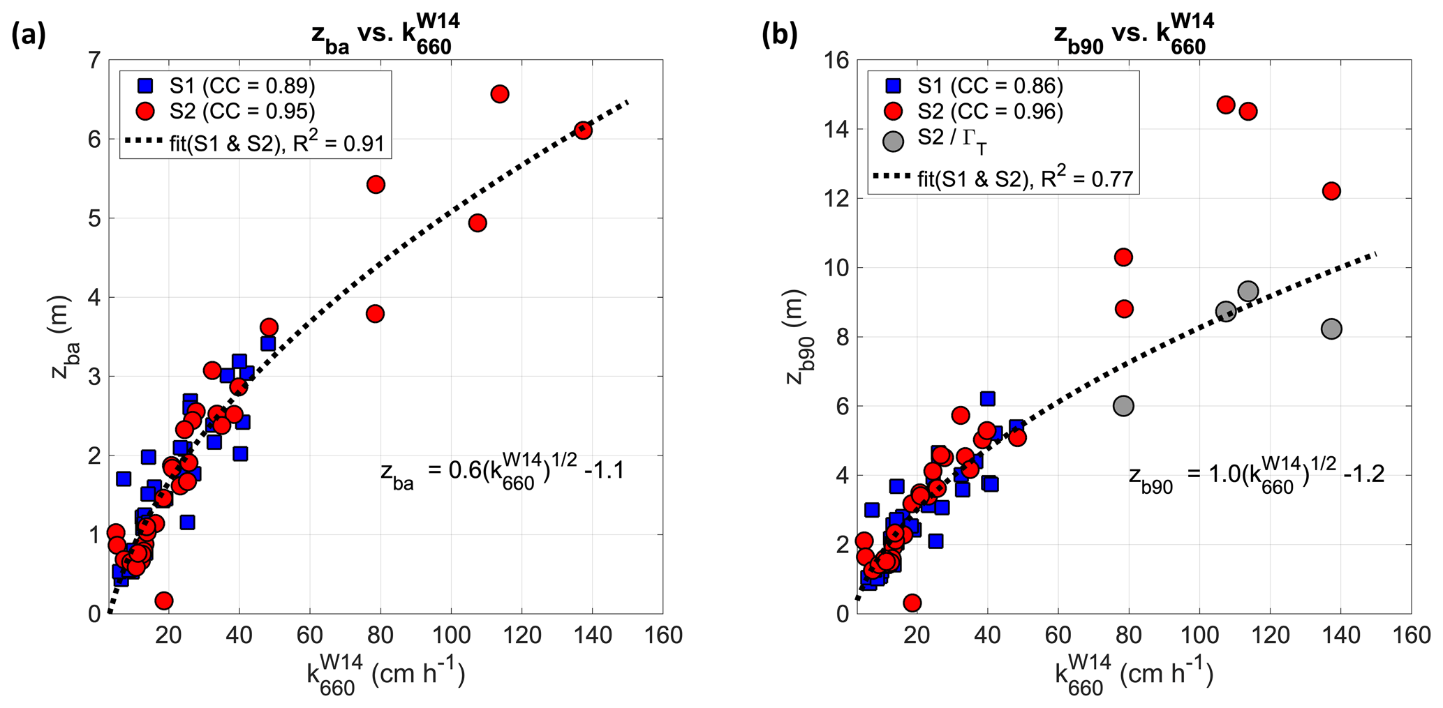
Figure 14 Relationship between wind-dependent parametrization of CO₂ gas transfer velocity $k_{\mathrm{660}}^{\text{w14}}$ and average (a) and 90th percentile (b) bubble depths. Empirical data from storms S1 (blue marker) and S2 (red marker) and curve of best fit for S1 and S2 data aggregated (dotted black curve; equation in the plot area). Grey markers indicate values across the peak of heat flux Q during S2 corrected with the stability parameter Γ_T.

With regard to z_ba (Fig. 14a), the correlation coefficient with k^W14 is high under both storms (CC=0.89 and 0.95 for S1 and S2, respectively), inheriting the good correspondence between z_ba and U₁₀. Given that W14 assumes a quadratic relationship with U₁₀, and z_ba linearly depends on U₁₀ with minor differences between S1 and S2, the transfer velocity $k_{\mathrm{660}}^{\text{w14}}$ (in cm h⁻¹) is related to z_ba (in m) with the following law (valid for U₁₀≥U_min):

$$\begin{array}{}\text{(14)}& z_{\text{ba}}=A{\left(k_{\mathrm{660}}^{\text{W14}}\right)}^{\mathrm{1}/\mathrm{2}}+M,\end{array}$$

by considering S1 and S2 data aggregated. The dimensional coefficients A=0.6 and $M=-\mathrm{1.1}$ were determined through nonlinear least square regression (the coefficient of determination R² equals 0.91). The behaviour is similar to that determined by Vagle et al. (2010), who showed the air flux F associated with bubble injection versus mean bubble penetration depth. A comparison with other experiments is not straightforward, since the coefficients A and M incorporate a sea-state dependence that is not explicit in W14.

A close relationship (R²>0.85) is also observed between $k_{\mathrm{660}}^{\text{W14}}$ and z_b90 (Fig. 14b). As above, a fitting is made considering only S2 data for which the thermal convection has had a minor role in driving the injection of bubbles. We find that the data fit well, whereas the depths across the peak of the storms are outliers. After being corrected with the water-column stability parameter Γ_T, bubble depth values across the peak of storm S2 tend to be reconciled with others and lie closer to the experimental curve. This result suggests a possible strategy that can be used to include in the gas transfer velocity formulae, like $k_{\mathrm{660}}^{\text{W14}}$, the effect of the stability of the water column, in terms of air–water temperature difference, which can lead to larger depths reached by air bubbles of any size.

Finally, the scatter between bubble depth and the bubble-mediated contribution to k by DM18 is shown in Fig. 15. Since the bubble-mediated gas transfer increases proportionately to whitecap coverage, implying a high transfer velocity in storm conditions (Woolf, 1997), we find that a strong connection exists between $k_{\text{b660}}^{\text{DM18}}$ and bubble depth (CC up to 0.92) and that storms S1 and S2 have similar distributions, for both the average and the 90th percentile of bubble depth. For both depths, a curve of the same type as in Eq. (14) provides a good fit over $k_{\mathrm{b}}^{\text{DM18}}$ by scaling the wind/wave forcing term $u_{\ast }^{\mathrm{5}/\mathrm{3}}(g{H}_{\mathrm{s}}{)}^{\mathrm{2}/\mathrm{3}}$ in Eq. (A5) with a square root law. As was done in the analysis of $k_{\mathrm{660}}^{\text{W14}}$, the use of a parameter like Γ_T tends to adjust the deeper depths experienced by air plumes during the cold-air outbreak, although we find that Γ_T values for $k_{\text{b660}}^{\text{DM18}}$ have to be reduced to about 25 % to fit the experimental data.

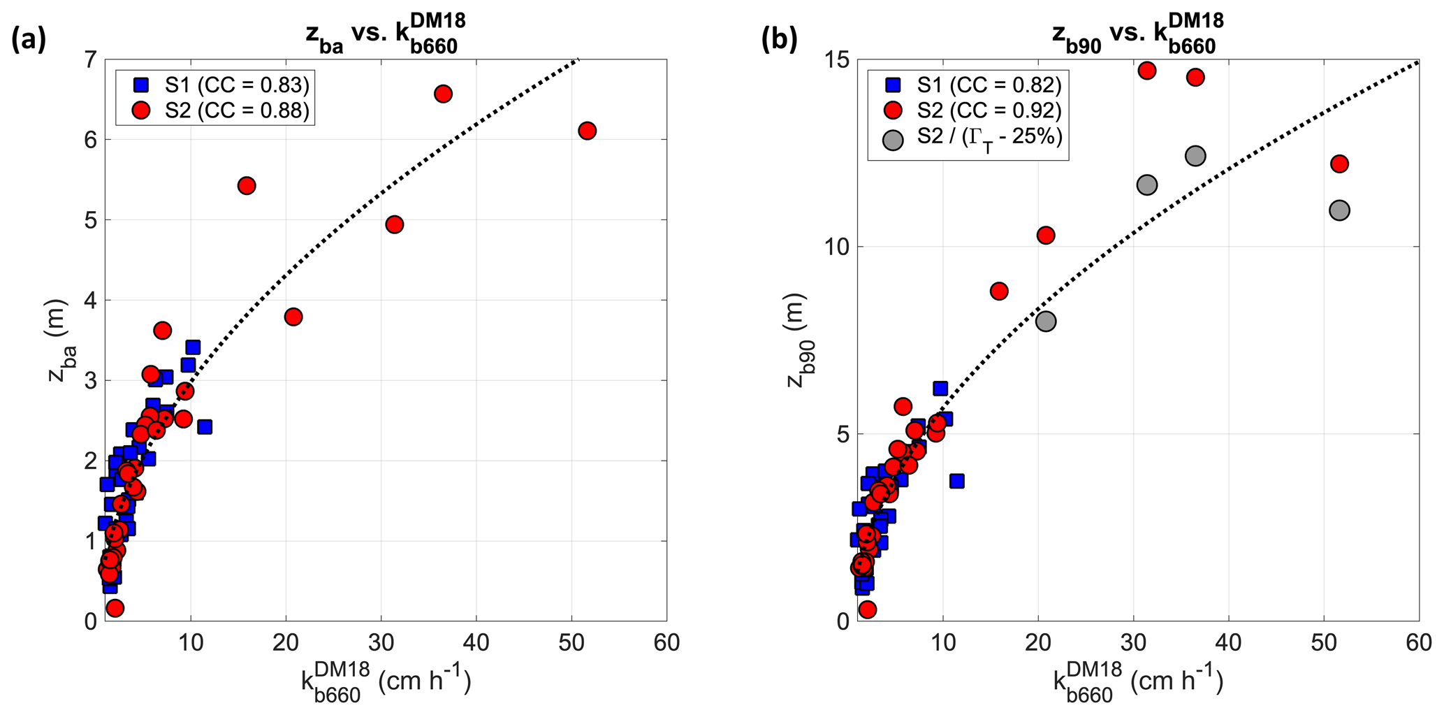
Figure 15 Relationship between bubble-mediated parametrization of CO₂ gas transfer velocity $k_{\text{b660}}^{\text{DM18}}$ and average (a) and 90th percentile (b) bubble depths. Data from storms S1 (blue marker) and S2 (red marker) and curve of best fit for S1 and S2 data aggregated (dotted black curve; equation in the plot area). Grey markers indicate values across the peak of heat flux Q during S2 corrected with the stability parameter Γ_T reduced empirically by 25 %.

5 Conclusions and outlook

In this paper, we have investigated a data set of observations of the air bubble plume and its penetration depth in the sea during two characteristic storms off the Venice littoral in the north Adriatic Sea (Italy). The analysis is made at the scale of the sea states and includes mixed-sea (wind–wave and swell) and unimodal wave conditions (wind–wave only). Underwater plumes have been inferred from the echo signal produced by a vertical-looking sonar operating at monochromatic 1000 kHz, which was deployed at a 17 m depth close to an oceanographic research tower that provided auxiliary observations. Bursts of 30 min acoustic backscatter profiles were analysed with the signal at a 2 Hz sample rate with vertical bins of 2.5 cm. The bubble penetration was identified in the plumes with an adaptive threshold approach and was analysed in wave-following coordinates. Two characteristic depths were investigated: the average and the 90th percentile, which have elucidated different mechanisms of the plume evolution. During the observational period, the total significant wave height peaked at about 3 m for both storms. Over the second storm, wind speed reached 26 m s⁻¹, and a cold-air outbreak event triggered heat fluxes up to 520 W m⁻² (the air temperature dropped to 2.6 °C). This combination caused cooling of the water masses whose presence was recorded close to the sea bottom at the sonar head. In search of a prediction law for the penetration of bubbles during storms, bubble-depth data have been parametrized against wind and wave forcings. Further, bubble plumes have been qualified in formulations of CO₂ air–sea fluxes using the transfer velocity as the variable of interest. The main observational findings and inference of the study are summarized as follows:

• Shallow and deep bubble plumes demonstrate a short time response and direct connection with the surface forcings. In line with previous studies that analysed the bubble penetration depths in the ocean, we have found that bubble penetrations follow an empirical linear law with wind speed closely, although the difference in the wind-speed regime and wave development between the two storms of this study. The minimum wind speed for bubble plumes to be generated is around 3 m s⁻¹. When compared with previous parametrizations of the same type, the data display smaller penetration depths for a given wind speed, which we considered to be due to the limited growth of waves in the north Adriatic Sea. When the wave forcing is incorporated in the assessment using a scaling with the wind/wave Reynolds number, a reconciliation between data sets collected at different locations and sea-state severity seems plausible.

• During the second storm (S2) of this study, we documented a large air–sea temperature difference that led to the cooling of waters and an intensification of the downward thermal convection. Although it is not a new phenomenon to describe, we recognize that it strongly affects the larger bubble depths, whose enhancement can be parametrized at the leading order by the air–sea temperature difference. After being corrected for the stability parameter proposed by Thorpe (1982), the bubble depth data were reconciled with others measured during other phases of the same storm and those from the first storm (S1) when heat fluxes were small.

• During the intense heat-flux phase of the second storm (S2), the bubble plume reached the seabed (17 m) and its depth exceeded 6H_s; otherwise, the maximum depths were at about half of the water column. The bubble depths followed a lognormal distribution, suggesting that a set of independent forces are at play simultaneously that determine the depths reached by the bubbles. However, the sonar used here did not make it possible to separate the contributions from different sources. Deeper and denser bubble plumes were accompanied by vertical convection with a downward maximum speed of 7 cm s⁻¹.

• The transfer velocity k of CO₂ gas was estimated from measured data using wind-only and wind/wave semi-empirical parametrizations. During the two storms S1 and S2, values of k reached 40 and 100 cm h⁻¹, respectively, with small differences between predictions from the wind-dependent Wanninkhof (2014) model and the wind/wave-dependent Deike and Melville (2018) model. Differences from the latter exceeding 10 cm h⁻¹ were found during S1 using the predictions of Brumer et al. (2017a). The bubble-mediated contribution to k was remarkable during S2, up to 40 cm h⁻¹, according to Deike and Melville (2018).

• By using the penetration depth of bubble plumes as a proxy for the intensity of the surface processes (wind and waves), we found a strong correlation between plume depth and theoretical CO₂ transfer velocity. This result was found for estimates of the total and the bubble-mediated contributions to k and for the average and extreme penetration depths, except for those values measured during the sinking of cold-water masses. In these conditions, the scaling of k with a stability parameter provides a possible means to include the thermal convection effects in the air–sea exchange of CO₂ gas. Results point in the direction that improved parametrizations of gas fluxes across the air–sea surface are needed to predict the future uptake of these gases by the oceans.

For future research, more accurate estimates of total and bubble-mediated gas transfer will benefit from measurements of the distribution of bubble size in the upper ocean and studies of the behaviour of bubbles under waves. Equipment that integrates vertical-looking sonar is required, for instance with above-water stereo cameras capable of providing breaking probability, whitecap coverage, and space–time wave geometry. For sonars, a standardization of the methodology to measure the edge of the bubble plume is recommended in order to ease the comparison of data collected with instruments with different carrier frequencies.

Appendix A: Parametrization of the air–sea transfer velocity of CO₂ gas

A1 Wind-dependent parametrization

For its effectiveness and confirmed by results from laboratory and field studies with gases of low solubility such as CO₂, the total transfer velocity k in Eq. (12) has been parametrized retaining only the influence of the momentum transfer from the wind, bypassing in this way the explicit role of other processes (surface waves and turbulence, for instance). Most commonly, a quadratic wind speed parametrization was used (Broecker et al., 1986; Sweeney et al., 2007; Wanninkhof, 1992), which was tuned to match the result for the global radiocarbon carbon budget over long-term timescales (Sweeney et al., 2007; Wanninkhof, 1992, 2014). In this study, we consider the relationship with coefficients calibrated by Wanninkhof (2014) given by

$$\begin{array}{}\text{(A1)}& k^{\text{W14}}=\mathrm{0.251}{U}_{\text{10n}}^{\mathrm{2}}{\left({\displaystyle \frac{\mathit{Sc}}{\mathrm{660}}}\right)}^{-\mathrm{1}/\mathrm{2}},\end{array}$$

where the units of k^W14 are in cm h⁻¹, and U_10n (in m s⁻¹) is the neutral stability wind speed at 10 m height. From a mechanistic standpoint, the quadratic dependencies suggest that gas exchange is roughly related to the momentum flux at the ocean surface. The strong wind-speed dependence implies that most transfers will occur in fairly high winds despite their relative rarity. Parametrization W14 does not separate the contribution to the total gas flux into the bubble gas transfer and the diffusive transfer at an unbroken surface. For CO₂, W14 provides good estimates for intermediate winds. At low winds with a smooth water surface, the quadratic relationship will underestimate gas transfer; at high winds, bubble-mediated exchange will affect gases differently depending on their solubility, and the relationship is only suitable for CO₂. For their relatively simple functional form, wind-dependent formulations are used by large-scale ocean and climate communities; for instance k^W14 is adopted for biogeochemistry numerical modelling by the European Copernicus Marine Service (https://resources.marine.copernicus.eu/products, last access: 29 April 2024; e.g., Teruzzi et al., 2021).

A2 Wind/wave-dependent parametrizations

CO₂ flux observations display substantial scatter at moderate to high wind speed, and wind-dependent parametrizations tend to diverge (Brumer et al., 2017a; Deike and Melville, 2018). This effect can be attributed to the wave conditions, which can vary for a given wind speed. The complex interplay of wind and waves in determining the interaction between the atmosphere and the sea implies that wind speed alone cannot capture the entire variability of air–sea CO₂ exchange, particularly wave breaking and its bubble production that can significantly enhance the gas exchange (Woolf, 1997). Breaking-induced bubbles offer an additional pathway for gas transfer between the atmosphere and ocean in addition to direct diffusion across the interface. Their influence increases with decreasing solubility, leading to a significant enhancement in the transfer of slightly soluble gases such as CO₂. The effect of breaking waves was initially considered in the bubble-mediated gas flux model by Keeling (1993). The gas transfer velocity from the bubbles to the ocean is mediated by an efficiency factor, which integrates the amount of gas each bubble transfers. The efficiency is expressed in terms of the characteristic depth of the bubble population and an equilibrium depth, and larger efficiencies, hence transfers, are obtained for greater bubble depths. In other words, deep bubble plumes provide a medium for efficient gas exchange. As for the surface manifestation of breaking-produced bubbles (whitecaps), efforts were made in the past to relate the breaking-mediated gas exchange to wind and wave forcings.

A bulk parametrization aimed at including the wave-related process in the CO₂ flux estimate was developed by Brumer et al. (2017a). They assumed that the whitecap fraction on the water surface is the primary process that quantifies the strength of wave breaking. The CO₂ gas transfer velocity data were fitted by Brumer et al. (2017a) using H_s computed from the total wave spectrum as

$$\begin{array}{}\text{(A2)}& k^{\text{B17}}=\mathrm{2.04}\times {\mathrm{10}}^{-\mathrm{4}}{R}_{\text{H}}^{\mathrm{0.88}}{\left({\displaystyle \frac{\mathit{Sc}}{\mathrm{660}}}\right)}^{-\mathrm{1}/\mathrm{2}},\end{array}$$

in units of m s⁻¹. In swell/wind–sea bimodal sea conditions, to account for only the active part of the wave field in generating whitecaps, Brumer et al. (2017a) isolated the wind–sea mode (denoted by “ws” subscript) of the wave spectrum and found the following relationship:

$$\begin{array}{}\text{(A3)}& k_{\text{ws}}^{\text{B17}}=\mathrm{1.64}\times {\mathrm{10}}^{-\mathrm{2}}{R}_{\text{H,ws}}^{\mathrm{0.59}}{\left({\displaystyle \frac{\mathit{Sc}}{\mathrm{660}}}\right)}^{-\mathrm{1}/\mathrm{2}},\end{array}$$

which suggests a near-quadratic dependence on wind speed. Brumer et al. found a similar performance in determining the transfer velocity from the total or the wind–sea significant wave height and argued that non-breaking waves (from swell) contribute to the wave-induced mixing and upper ocean turbulence. Similar parametrizations that used a power law of the wind–wave Reynolds number for k were developed in the studies by Zhao et al. (2003), Woolf (2005), and Jähne et al. (1985). Further, based on laboratory experiments, the dependence on the wind–wave Reynolds number was adjusted to include the wave orbital motion for scaling the efficiency of generating turbulence (Li et al., 2021).

A different approach for the characterization of the breaking-mediated flux has been considered in the spectral model by Deike and Melville (2018), in which the CO₂ total gas transfer velocity k is separated into non-bubble (k_nb) and bubble-mediated (k_b) contributions, that is

$$\begin{array}{}\text{(A4)}& k^{\text{DM18}}=k_{\mathrm{b}}^{\text{DM18}}+k_{\text{nb}}^{\text{DM18}}.\end{array}$$

The breaking term arises from the scaling of the breaking probability density function and gives a different weight to u_∗ and H_s. The most important part of the wave spectrum for gas transfer is the saturation range, where breaking dominates the energy balance. Based on this consideration, the value of k_b was formulated semi-empirically by Deike and Melville (2018) using the product of bulk variables in the following form:

$$\begin{array}{}\text{(A5)}& k_{\mathrm{b}}^{\text{DM18}}={\displaystyle \frac{A_B}{K_{\text{0}}R{T}_{\mathrm{0}}}}{u}_{\ast }^{\mathrm{5}/\mathrm{3}}(g{H}_{\mathrm{s}}{)}^{\mathrm{2}/\mathrm{3}}{\left({\displaystyle \frac{\mathit{Sc}}{\mathrm{660}}}\right)}^{-\mathrm{1}/\mathrm{2}},\end{array}$$

where $A_B={\mathrm{10}}^{-\mathrm{5}}$ s² m⁻² is a dimensional fitting coefficient, K₀ is the CO₂ solubility in seawater, T₀ is the sea surface temperature, and R is the ideal gas constant. The general idea behind the DM18 model is that both wind friction and waves must be present for the bubble-mediated flux to be effective. The formula in Eq. (A5) proved efficient in reducing the scatter of wind-based gas transfer velocity parametrizations. However, other wave-field characteristics related to the wave-breaking tendency, such as the wave steepness or period, were not explicitly included. The bubble contribution (Eq. A5) to total gas transfer is stronger in high wind and wave conditions, when the wave energy and air entrainment are larger, and as the wave field develops. It is estimated that bubble-mediated transfer is the dominant mechanism in open-ocean conditions where the wind speed exceeds 17 m s⁻¹ (Reichl and Deike, 2020). Recent analyses suggested modulation of the bubble-mediated contribution by current gradients, which is significant along sub-mesoscale fronts and cold filaments. There, wave breaking can be enhanced by the wave-energy focus by current-induced refraction and the direct forcing by the current gradients (Shin et al., 2022).

The non-bubble contribution is led by diffusive mass transfer at the unbroken, smooth air–sea interface (i.e. no whitecapping), which wind-driven turbulence enhances. It was found to scale linearly with the friction velocity u_∗ (Jähne et al., 1987) and is integrated in the Deike and Melville model using the COARE 3.1 parametrization (Fairall et al., 2011) as follows:

$$\begin{array}{}\text{(A6)}& k_{\text{nb}}^{\text{DM18}}=A_{\text{NB}}{u}_{\ast }{\left({\displaystyle \frac{\mathit{Sc}}{\mathrm{660}}}\right)}^{-\mathrm{1}/\mathrm{2}},\end{array}$$

where $A_{\text{NB}}=\mathrm{1.55}\times {\mathrm{10}}^{-\mathrm{4}}$ is an empirical, non-dimensional coefficient (the unit of $k_{\text{nb}}^{\text{DM18}}$ is the same as u_∗).

An alternative parametrization of the total gas transfer velocity was developed in the context of the COAREG 3.6 bulk air–sea flux algorithm (Fairall et al., 2022). In COAREG 3.6, it is assumed that the bubble-mediated transfer velocity is directly related to white capping coverage as follows (Woolf, 1997):

$$\begin{array}{}\text{(A7)}& k_{\mathrm{b}}^{\text{W97}}=B\cdot \mathrm{2450}{f}_{\mathrm{w}}/\left\{\mathit{\beta }[\mathrm{1}+(\mathrm{14}\mathit{\beta }{\mathit{Sc}}^{-\mathrm{0.5}}{)}^{-\mathrm{1}/\mathrm{1.2}}{]}^{\mathrm{1.2}}\right\},\end{array}$$

where B=2.5 is an empirical constant tuned by Fairall et al. (2022), f_w is the whitecap fraction, and β is the Oswald solubility. The whitecap scaling is a surrogate for the production and mixing of bubbles. The original model by Woolf assumed the whitecap fraction scaling with neutral wind speed, while in COAREG 3.6, the wind–wave Reynolds number parametrization of whitecap coverage (%) is used in the form of Brumer et al. (2017b).