The different dynamic influences of Typhoon Kalmaegi on two pre-existing anticyclonic ocean eddies

Using multi-source observational data and GLORYS12V1 reanalysis data, we conduct a comparative analysis of different responses of two warm eddies, AE1 and AE2 in the northern South China Sea, to Typhoon Kalmaegi during September 2014. The findings of our research are as follows: (1) for horizontal distribution, the area and the sea surface temperature (SST) of AE1 and AE2 decrease by about 31 % (36 %) and 0.4 °C (0.6 °C). The amplitude, Rossby number (Ro = relative vorticity $/$ Coriolis parameter) and eddy kinetic energy (EKE) of AE1 increase by 1.3 cm (5.7 %), $\mathrm{1.4}\times {\mathrm{10}}^{-\mathrm{2}}$ (20.6 %) and 107.2 cm² s⁻² (49.2 %) after the typhoon, respectively, while AE2 weakens and the amplitude, Rossby number and EKE decrease by 3.1 cm (14.6 %), $\mathrm{1.6}\times {\mathrm{10}}^{-\mathrm{2}}$ (26.2 %) and 38.5 cm² s⁻² (20.2 %), respectively. (2) In the vertical direction, AE1 demonstrates enhanced convergence, leading to an increase in temperature and a decrease in salinity above 150 m. The response below the mixed-layer depth (MLD) is particularly prominent (1.3 °C). In contrast, AE2 experiences cooling and a decrease in salinity above the MLD. Below the MLD, it exhibits a subsurface temperature drop and salinity increase due to the upwelling of cold water induced by the suction effect of the typhoon. (3) The disparity in the responses of the two warm eddies can be attributed to their different positions relative to Typhoon Kalmaegi. Under the influence of negative wind stress curl outside the maximum wind radius (R_max) of the typhoon, triggering negative Ekman pumping velocity (EPV) and quasi-geostrophic adjustment of the eddy, the warm eddy AE1, with its center to the left of the typhoon's path, further enhances the converging sinking of the upper warm water, resulting in its intensification. On the other hand, the warm eddy AE2, situated closer to the center of the typhoon, weakens due to the cold suction caused by the strong positive wind stress curl within the typhoon's R_max. The same polarity eddies may have different response to typhoons. The distance between eddies and typhoons, eddy intensity, and the background field need to be considered.

1 Introduction

Tropical cyclones (TCs), as they traverse the vast ocean, interact with oceanic mesoscale processes, particularly with mesoscale eddies, representing a crucial aspect of air–sea interaction (Shay and Jaimes, 2010; Lu et al., 2016; Song et al., 2018; Ning et al., 2019; Sun et al., 2023). The South China Sea (SCS) experiences an average of six TCs passing through each year (Wang et al., 2007), causing prominent exchange of energy and mass between the air and sea (Price, 1981). Meanwhile, due to the influence of the Asian monsoon, intrusion of the Kuroshio Current and complex topography, the northern South China Sea (NSCS) also encounters frequent eddy activities (Xiu et al., 2010; Chen et al., 2011). These mesoscale oceanic eddies often play significant roles in mass and heat transport and air–sea interaction. This unique setting offers an exceptional opportunity to investigate the generation, evolution and termination of mesoscale eddies and their interaction with TCs.

Pre-existing mesoscale eddies play a crucial role in the feedback mechanism between the ocean and TCs. Cyclonic eddies (cold eddies) enhance the sea surface cooling effect under TC conditions, resulting in TCs weakening due to their thermodynamic structures and cold-water entrainment processes that reduce the heat transfer from the sea surface to the TCs through air–sea interaction (Ma et al., 2017; Yu et al., 2021). In contrast, anticyclonic eddies (warm eddies) suppress this cooling effect, leading to TC intensification (Shay et al., 2000; Walker et al., 2005; Lin et al., 2011; Wang et al., 2018). Warm eddies have a thicker upper mixed layer, which stores more heat. When a TC passes over a warm eddy, it increases sensible heat and water vapor in the TC's center, both of which are closely related to the TC's intensification (Wada and Usui, 2010; Huang et al., 2022). Furthermore, the downwelling within warm eddies hinders the upwelling of cold water, reducing the apparent sea surface cooling caused by the TCs. These processes weaken the oceanic negative feedback effect and help to sustain or even strengthen TC development.

On the other hand, TCs also have a notable impact on the intensity, size and movement of mesoscale eddies. In some cases, TCs strengthen cold eddies and can even lead to the formation of new cyclonic eddies in certain situations (Sun et al., 2014), while they also accelerate the dissipation of anticyclonic eddies (Zhang et al., 2020). The strengthening effect of TCs on cold eddies is related to the positions between cold eddies and TCs, the intensity of eddies, and the TC-induced geostrophic response (Lu et al., 2016, 2023; Yu et al., 2019). Cyclonic eddies on the left side of the TC's track are more intensely affected by the TC, and eddies with shorter lifespans or smaller radii are more susceptible to the influence of TCs. The dynamic adjustment process of eddies and the upwelling induced by TCs themselves lead to changes in the three-dimensional structure of the cyclonic eddies, including ellipse deformation and re-axisymmetrization on the horizontal plane, resulting in eddy intensification. The presence of cold eddies not only exacerbates the sea surface cooling in the post-TC cold-eddy region but also accompanies a decrease in the sea level anomaly (SLA), deepening of the mixed layer, a strong cooling in the subsurface, increased chlorophyll-a concentration within the eddy, and substantial increases in EKE and available potential energy (Shang et al., 2015; Liu and Tang, 2018; Li et al., 2021; Ma et al., 2021).

Generally, TCs lead to a weakening of warm eddies, while the sea surface cooling is not significant, typically within 1 °C. However, there is a noticeable cooling and increased salinity in the subsurface layer, accompanied by an upward shift of the 20 °C isotherm and a decrease in heat and kinetic energy (Lin et al., 2005; Liu et al., 2017; Huang and Wang, 2022). Lu et al. (2020) propose that TCs primarily generate potential vorticity input through the geostrophic response. When a TC passes over an eddy, there is a significant positive wind stress curl within the TC's maximum wind radius (R_max), which induces upwelling in the mixed layer due to the divergence of the wind-driven flow field. This upward flow compresses the thickness of the isopycnal layers below the mixed layer, resulting in a positive potential vorticity anomaly. Rudzin and Chen (2022) found that under the interaction of the strong TC wind stress in the eye area of the TC and the subsurface ocean current, the positive vertical vorticity advection caused the TC to eliminate the warm eddy from the bottom to top after passing through. However, the projection of TC wind stress onto the eddy and the relative position of the warm eddy to the TC can lead to different responses. According to the classical description of TC-induced upwelling, strong upwelling occurs within 2×R_max of the TC center, while weak subsidence exists in the vast area outside the upwelling region (Price, 1981; Jullien et al., 2012). The warm eddy located directly beneath the TC's path weakens due to the cold suction caused by the TC's center. However, for warm eddies located beyond 2×R_max, they are influenced by the TC's wind stress curl and the downwelling within the eddy itself, resulting in the convergence of warm water in the upper layers of the eddy, an increase in mixed-layer thickness and an increase in heat content, in turn leading to a warming response to the TC (Jaimes and Shay, 2015).

The NSCS encounters high-frequency and intense TCs; concurrently, there is notable activity of mesoscale eddies in this region. Based on in situ datasets, multi-platform satellite measurements and GLORYS12V1 reanalysis data, we investigate how the upper ocean in two anticyclonic eddies responds to Typhoon Kalmaegi. This marks an initial effort to characterize the different physical variations induced by TCs within the same two polarity eddies, contributing to a better understanding of the role played by mesoscale eddies in modulating interactions between TCs and the ocean. Section 2 provides an overview of the data and methods utilized in this research. Section 3 analyzes the physical parameters of warm eddies, vertical temperature and salinity variations and explores the different responses of warm eddies both inside and outside the typhoon-affected region. Section 4 offers a comprehensive discussion, and Sect. 5 gives a summary.

2 Data and methods

2.1 Data

The 6-hourly best-track typhoon datasets are obtained from the Joint Typhoon Warning Center (JTWC; http://www.usno.navy.mil/JTWC, last access: 3 February 2021), the Japan Meteorological Agency (JMA; https://www.jma.go.jp/jma/jma-eng/jma-center/rsmc-hp-pub-eg/besttrack.html, last access: 3 February 2021) and the China Meteorological Administration (CMA; https://tcdata.typhoon.org.cn/, last access: 23 April 2024). The data contain the TCs' center locations, minimum central pressure, maximum sustained wind speed and intensity category. The translation speed of typhoons is calculated by dividing the distance traveled by each typhoon within a 6 h interval by the corresponding time. In this paper, Typhoon Kalmaegi and Tropical Storm Fung-wong are studied (Fig. 1).

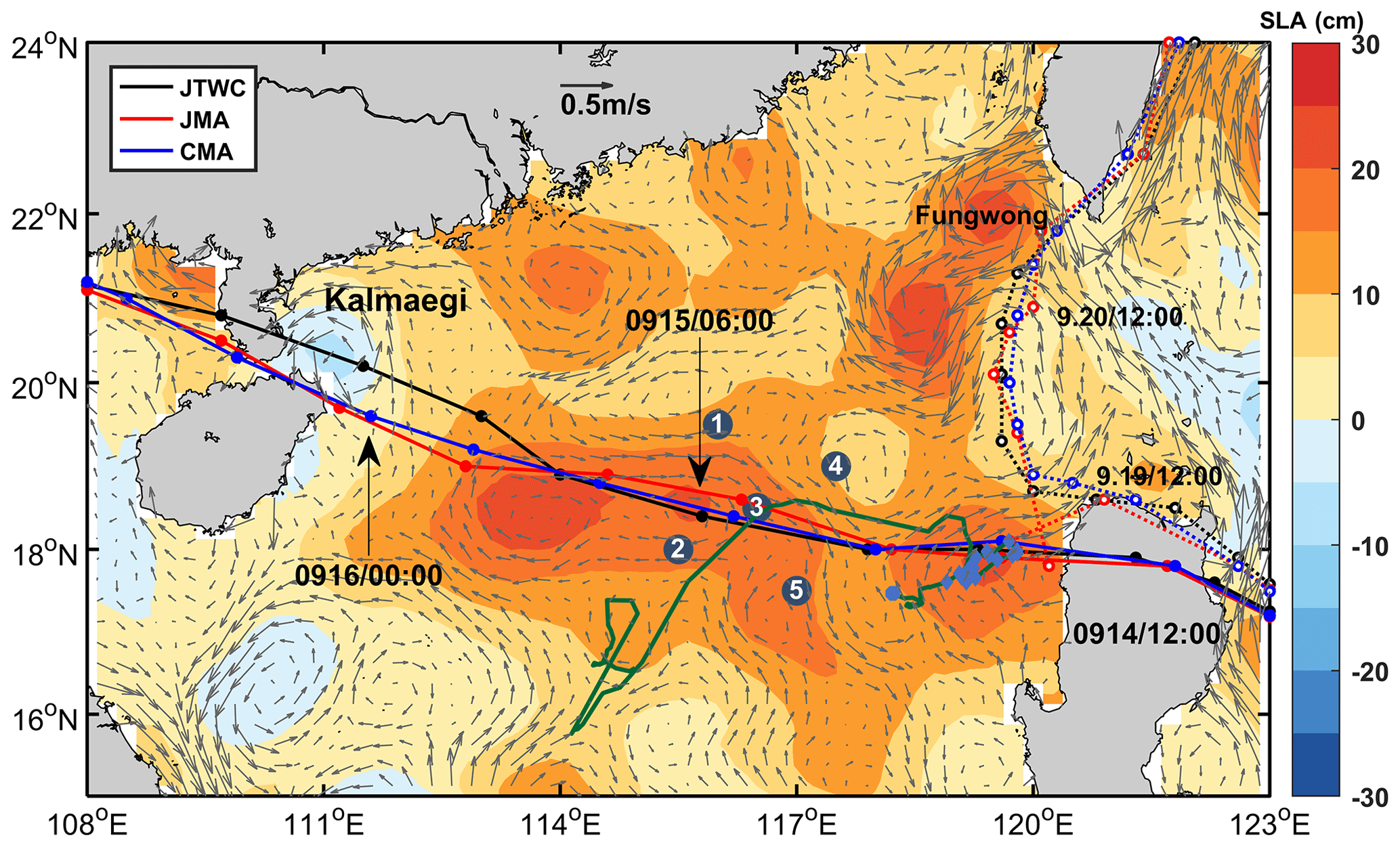
Figure 1 The tracks of Typhoon Kalmaegi (solid lines with filled dots) and Tropical Storm Fung-wong (dashed lines with unfilled dots) as provided by the Joint Typhoon Warning Center (JTWC, black), Japan Meteorological Agency (JMA, red) and China Meteorological Administration (CMA, blue). The color shading represents the sea surface level anomaly on 13 September 2014, while the gray arrows illustrate the geostrophic flow field. The numbered blue dots represent the positions of the five buoy and mooring stations, the green line illustrates the trajectory of Argo 2901469, and the blue diamonds mark the positions of Argo 2901469 inside the eddy AE2 from 26 August to 25 October 2014.

The daily sea level anomaly (SLA) and geostrophic current data are provided by the Archiving, Validation, and Interpretation of Satellite Oceanographic data (AVISO) product (Copernicus Marine Environment Monitoring Service (CMEMS); https://marine.copernicus.eu/, last access: 14 February 2022). This dataset combines satellite data from Jason-3, Sentinel-3A, HY-2A, SARAL/AltiKa, CryoSat-2, Jason-2, Jason-1, TOPEX/Poseidon (T/P), Envisat, GFO, and ERS-1 and ERS-2. The spatial resolution of the product is $\mathrm{1}/\mathrm{4}\mathit{°}\times \mathrm{1}/\mathrm{4}\mathit{°}$. The period from 1 September to 30 September 2014 was used.

The daily sea surface temperature (SST) data used in this study are derived from the Advanced Very High Resolution Radiometer (AVHRR) product data provided by the National Oceanic and Atmospheric Administration (NOAA). The data are obtained from the Physical Oceanography Distributed Active Archive Center (PO.DAAC) at the NASA Jet Propulsion Laboratory (JPL) (https://www.ncei.noaa.gov/products/avhrr-pathfinder-sst, last access: 23 April 2024). The spatial resolution of the data is $\mathrm{1}/\mathrm{4}\mathit{°}\times \mathrm{1}/\mathrm{4}\mathit{°}$.

Argo data, including profiles of temperature and salinity from the surface to 2000 m depth, are obtained from the real-time quality-controlled Argo database (Euro-Argo; https://dataselection.euro-argo.eu/, last access: 4 April 2022). We select Argo float number 2901469, situated in an anticyclonic eddy and in close proximity to Typhoon Kalmaegi, both before and after the typhoon's passage in 2014. Profiles of this Argo are also used to validate the vertical distribution of temperature and salinity from GLORYS12V1.

For this study, we also utilize in situ data from a cross-shaped array consisting of five stations, comprising five moored buoys and four subsurface moorings (refer to Fig. 1). More specific information can be found in Zhang et al. (2016). To investigate the impact of the typhoon on a warm eddy, we select the temperature and salinity data from Station 5, situated to the left of Kalmaegi's track.

The wind speed data are sourced from the European Centre for Medium-Range Weather Forecasts (ECMWF) ERA-Interim reanalysis assimilation dataset (https://cds.climate.copernicus.eu/cdsapp#!/dataset/reanalysis-era5-single-levels?tab=form, last access: 23 April 2024). We used the reanalysis data of surface winds at a height of 10 m above sea level for TCs. The selected data have a spatial resolution of $\mathrm{1}/\mathrm{4}\mathit{°}\times \mathrm{1}/\mathrm{4}\mathit{°}$ and a temporal resolution of 6 h, with four updates per day (00:00, 06:00, 12:00 and 18:00 UTC). The data correspond to September 2014.

The Global Ocean Physics Reanalysis product GLOBAL_MULTIYEAR_PHY_001_030 (GLORYS12V1), provided by CMEMS (https://marine.copernicus.eu/, last access: 23 April 2024) is used in this study too. This reanalysis product utilizes the NEMO 3.1 numerical model coupled with the LIM2 sea ice model and is forced with ERA-Interim atmospheric data. The model assimilated along-track altimeter data from satellite observations (Pujol et al., 2016), satellite sea surface temperature data from AVHRR, sea ice concentration from CERSAT (Ezraty et al., 2007), and vertical profiles of temperature and salinity from the CORAv4.1 database (Drévillon et al., 2021). The temperature and salinity biases were corrected using a 3D-Var scheme. GLORYS12V1 has a horizontal resolution of $\mathrm{1}/\mathrm{12}\mathit{°}\times \mathrm{1}/\mathrm{12}\mathit{°}$, and it has 50 vertical levels. The temperature, salinity and ocean mixed layers' thickness from 1 September to 30 September 2014 were chosen.

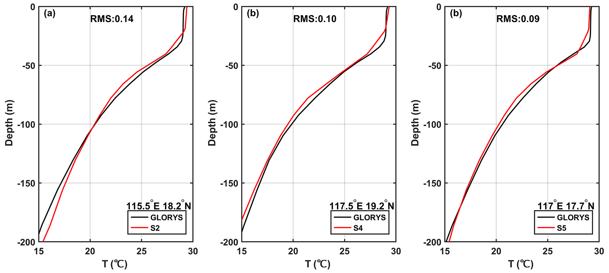
Figure 2 Evaluation of GLORYS12V1 data performance during September 2014. Panels (a), (b) and (c) are the comparison of vertical monthly mean temperatures recorded at Station 2 (18.2° N, 115.5° E), Station 4 (19.2° N, 117.5° E) and Station 5 (17.7° N, 117° E), respectively.

GLORYS12V1 is a widely used and applicable dataset; to evaluate its temperature profiles, in situ data of Station 2, Station 4 and Station 5 were compared (Fig. 2). Since the GLORYS12V1 data are assimilated with the data of Argo floats, they demonstrate good agreement with Argo profiling floats; the maximum difference between them is less than 0.2 °C, and the root mean square (rms) is 0.02 (figure not shown). However, there are some discrepancies between the GLORYS12V1 and the Station 5 data, with the largest difference occurring at the depths of 30 m (mixed layer) and 78 m (thermocline), both differing by 0.6 °C, while below 150 m, the difference is quite small. The rms is 0.09. The rms between GLORYS12V1 and Station 2 (Station 4) is 0.14 (0.10), with deviations in the mixed layer and thermocline, although compared to Station 5, the rms of Station 2 and Station 4 is a little larger but still acceptable. Overall, GLORYS12V1 reproduces the observed ocean temperature accurately, and it is reasonable to use it to investigate the vertical response of anticyclonic eddies to Typhoon Kalmaegi.

2.2 Methods

Vorticity is a vector that characterizes the local rotation within a fluid flow. Mathematically, it is defined as the curl of the velocity vector. In most cases, when referring to vorticity, it specifically pertains to the vertical component of the vorticity. It is calculated from

$$\begin{array}{}\text{(1)}& \mathit{\zeta }={\displaystyle \frac{\partial v}{\partial x}}-{\displaystyle \frac{\partial u}{\partial y}}.\end{array}$$

Here, u and v are the zonal (eastward) and meridional (northward) geostrophic velocities, respectively. They are derived from altimeter sea level anomaly data (η):

$$\begin{array}{}\text{(2)}& u=-{\displaystyle \frac{g}{f}}{\displaystyle \frac{\partial \mathit{\eta }}{\partial y}},v={\displaystyle \frac{g}{f}}{\displaystyle \frac{\partial \mathit{\eta }}{\partial x}}.\end{array}$$

Here, g is the acceleration of gravity and f is the Coriolis frequency. Vorticity is considered a fundamental characteristic of mesoscale eddies: positive vorticity signifies cyclonic eddies, while negative vorticity indicates anticyclonic eddies.

The Rossby number (Ro) is a dimensionless number describing fluid motion, and it is the ratio of relative vorticity to planetary vorticity, reflecting the relative importance of local non-geostrophic motion versus large-scale geostrophic motion. The larger the Rossby number, the stronger the local non-geostrophic effect, and the definition of this parameter is

$$\begin{array}{}\text{(3)}& \mathit{Ro}={\displaystyle \frac{\mathit{\zeta }}{f}}.\end{array}$$

Eddy kinetic energy (EKE) is a measure of the energy associated with mesoscale eddies and indicates the intensity of eddies. It is typically calculated using the anomalies of the geostrophic velocity:

$$\begin{array}{}\text{(4)}& \text{EKE}={\displaystyle \frac{\mathrm{1}}{\mathrm{2}}}(u^{{\prime }^{\mathrm{2}}}+v^{{\prime }^{\mathrm{2}}}),\end{array}$$

where u^′ represents the anomaly of the geostrophic zonal (eastward) velocity, v^′ represents the anomaly of the meridional (northward) velocity. The geostrophic velocity anomalies are referenced to the period of 1993 to 2012.

To evaluate the impact of a typhoon on an anticyclonic eddy, the calculation begins with determining the wind stress:

$$\begin{array}{}\text{(5)}& \mathit{\tau }={\mathit{\rho }}_{\mathrm{a}}{C}_{\mathrm{d}}{U}_{\mathrm{10}}{\mathit{U}}_{\mathbf{10}},\end{array}$$

where ρ_a is the air density, assumed to be a constant value of 1.293 kg m⁻³, and U₁₀ represents the 10 m wind speed. C_d is the drag coefficient at the sea surface (Oey et al., 2006):

$$\begin{array}{c}{\displaystyle }{C}_{\mathrm{d}}\times {\mathrm{10}}^{\mathrm{3}}=\\ \text{(6)}& {\displaystyle }\left\{\begin{array}{ll}\mathrm{1.2}& U_{\mathrm{10}}\le \mathrm{11}\mathrm{m}{\mathrm{s}}^{-\mathrm{1}}\\ \mathrm{0.49}+\mathrm{0.065}{U}_{\mathrm{10}}& \mathrm{11}<U_{\mathrm{10}}\le \mathrm{19}\mathrm{m}{\mathrm{s}}^{-\mathrm{1}}\\ \mathrm{1.364}+\mathrm{0.0234}{U}_{\mathrm{10}}-\mathrm{0.0002}{U_{\mathrm{10}}}^{\mathrm{2}}& \\ & \mathrm{19}<U_{\mathrm{10}}\le \mathrm{100}\mathrm{m}{\mathrm{s}}^{-\mathrm{1}}.\end{array}\right.\end{array}$$

The wind stress curl is calculated by (Kessler, 2006)

$$\begin{array}{}\text{(7)}& \text{curl}\left(\mathit{\tau }\right)={\displaystyle \frac{\partial {\mathit{\tau }}_y}{\partial x}}-{\displaystyle \frac{\partial {\mathit{\tau }}_x}{\partial y}},\end{array}$$

where τ_x and τ_y are the eastward and northward wind stress vector components, respectively. The curl represents the rotation experienced by a vertical air column in response to spatial variations in the wind field.

The Ekman pumping velocity (EPV) represents the ocean upwelling rate, which can be used to study the contribution of typhoons to regional ocean upwelling. Positive values represent upwelling, and negative values represent downwelling:

$$\begin{array}{}\text{(8)}& \text{EPV}=\text{curl}\left({\displaystyle \frac{\mathit{\tau }}{\mathit{\rho }f}}\right),\end{array}$$

where the wind stress is obtained from Eq. (7); ρ is seawater density, with a value of 1025 kg m⁻³; and f is the Coriolis frequency.

The buoyancy frequency is a measure of the degree to which water is mixed and stratified. In a stable temperature stratification, the fluid particles move in the vertical direction after being disturbed, and the combined action of gravity and buoyancy always makes them return to the equilibrium position and oscillate due to inertia. When N²<0, the water is in an unstable state:

$$\begin{array}{}\text{(9)}& N^{\mathrm{2}}=-{\displaystyle \frac{g}{\mathit{\rho }}}{\displaystyle \frac{\partial \mathit{\rho }}{\partial z}},\end{array}$$

where ρ is seawater density, g is the acceleration of gravity, and z is the depth.

3 Results

3.1 Typhoon and pre-existing eddies in the NSCS

3.1.1 Track of Typhoon Kalmaegi and Tropical Storm Fung-wong

Typhoon Kalmaegi strengthened into a typhoon by 12:00 UTC on 13 September and emerged over the warm waters of the northern South China Sea (NSCS) by 15:00 UTC on 14 September, with maximum sustained winds of 33 m s⁻¹ (Fig. 3). During this period, the NSCS experienced predominantly weak vertical wind shear and was characterized by multiple anticyclonic warm eddies (Fig. 3). Subsequently, Typhoon Kalmaegi underwent two rapid intensification phases between 15 and 16 September. The first intensification occurred at 00:00 UTC on 15 September, propelling Kalmaegi to category 1 status with surface winds surpassing 35 m s⁻¹. By 12:00 UTC on 15 September, Kalmaegi experienced a second, even more rapid intensification, with winds reaching 40 m s⁻¹ in less than 12 h. Throughout this intensification stage, Kalmaegi encountered two warm eddies: anticyclonic eddy AE1, positioned to the left of the typhoon's path with its core situated on the periphery of the typhoon's 1×R_max (Fig. 3c and d). AE1 had a lifespan of 105 d from 26 June to 8 October and was positioned at 17–20° N, 113–116° E. AE2 precisely intersects with the typhoon's trajectory, and its core nearly coincides with the R_max of the typhoon (Fig. 3b–d). It had a lifespan of 89 d from 24 August to 20 November and was located at 17–19° N, 118–120° E. Kalmaegi made landfall on the island of Hainan at 03:00 UTC on 16 September, with a minimum central pressure of 960 hPa and a maximum wind speed of 40 m s⁻¹. After landfall, Typhoon Kalmaegi gradually weakened and dissipated. During its crossing of the NSCS, the five mooring stations were affected. Stations 1 and 4 were on the right side of Typhoon Kalmaegi's track, while Stations 2 and 5 were on the left side. Unfortunately, the wire rope of the buoy at Station 3 was destroyed by Kalmaegi, resulting in missing data from 15 September. Among the stations, Station 5 was on the left of the typhoon track and outside AE2, so its data are used in our study.

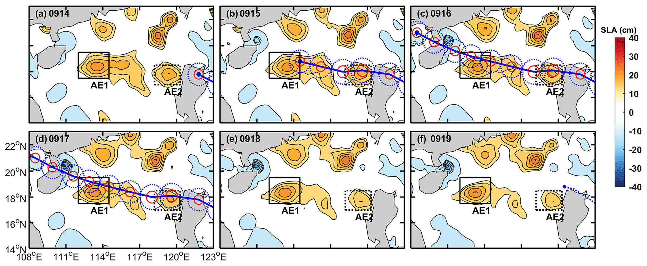
Figure 3 The variations in sea level anomaly before and after Typhoon Kalmaegi moved over the anticyclonic eddies AE1 and AE2 between 14 September and 19 September (a–f). The solid black rectangle represents the area of AE1, while the dashed black rectangle represents the area of AE2. The solid blue line depicts the path of Typhoon Kalmaegi, the solid red and dashed blue circles are the 1×R_max of the typhoon and width of the typhoon-induced baroclinic geostrophic response, and the dotted blue line in (f) is the path of Tropical Storm Fung-wong (best-track data sourced from CMA).

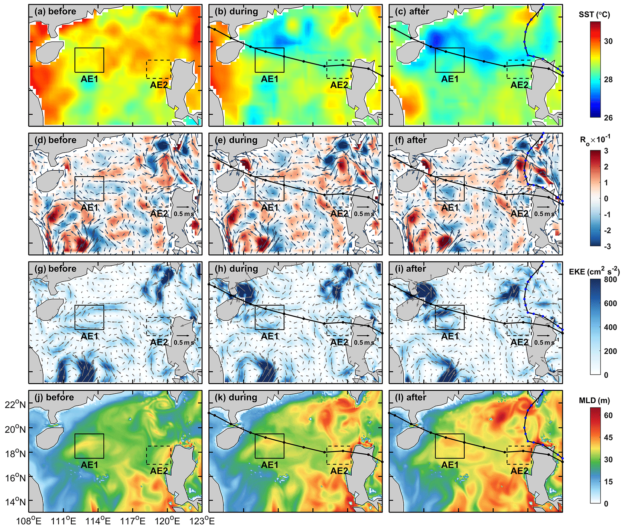
Figure 4 The spatial distribution of SST, Ro, EKE and mixed-layer depth (MLD) before, during and after the passage of TCs. The time periods of 10–13, 15–16 and 19–22 September are designated as stages before, during and after Kalmaegi, respectively. The path of Typhoon Kalmaegi is depicted by a solid black line with black dots, while the path of Tropical Storm Fung-wong is represented by a solid black line with blue dots in the third column. The solid and dashed boxes correspond to AE1 and AE2, respectively.

Tropical Storm Fung-wong initially moved quickly in a northwest direction after formation. On 19 September, it entered the Luzon Strait and decelerated. It made landfall in Taiwan on 21 September and subsequently landed in Zhejiang on 22 September before gradually dissipating. When crossing the Luzon Strait at 12:00 UTC on 19 September, anticyclonic eddy AE2 was on the left side of Fung-wong, with a distance of just over 100 km from its center.

3.1.2 Eddy characteristics' distribution

Satellite SLA measurements have proven to be highly effective and widely used for identifying and quantifying the intensity of ocean eddies (Li et al., 2014). In Fig. 3, two warm eddies with a clear positive (> 13 cm) SLA are observed along Typhoon Kalmaegi's track. During the period of 15 to 16 September, the typhoon passed over two warm anticyclonic eddies, AE1 and AE2. Before the typhoon, AE1 was the most prominent eddy in the SCS, with an amplitude of 23.0 cm and a radius of 115.5 km. AE2, located west of the island of Luzon, had an amplitude of 21.2 cm, with a radius of approximately 65.5 km. Tracing back 2 months (figure not shown), AE1 propagated slowly westward with about 0.1 m s⁻¹, while AE2 was generated on 24 August. From 14 to 19 September, the amplitude of AE1 increased by 1.3 cm. The area of AE1 decreased by approximately 31 % from 1.3×10⁵ to 9.1×10⁴ km² and split into two eddies. When Typhoon Kalmaegi crossed the core of AE2 at 15:00 UTC on 14 September and Tropical Storm Fung-wong moved over the northeast of AE2 at 12:00 UTC on 19 September, the amplitude decreased by 3.1 cm. The area of AE2 decreased by approximately 36 % from 4.2×10⁴ to 2.7×10⁴ km².

Because of intense solar radiation in September, the SST in the SCS was generally above 28.5 °C prior to the arrival of Typhoon Kalmaegi (Fig. 4a). As a fast-moving typhoon with a mean moving speed of over 8 m s⁻¹, Kalmaegi induced a larger cooling area and intensity on the right side of its path compared to the left side (Price, 1981). During the passage of Kalmaegi, the lowest SST on the right side of typhoon decreased to 27.2 °C. Even after the typhoon had passed, a cold wake could still be observed on the right side of its path, persisting for over a week (Fig. 4c).

The pre-existing warm eddy AE1 began to cool down before Kalmaegi reached the NSCS, dropping to 28.4 °C on 14 September. During this period, the mean SST within AE1 increased slightly to 28.6 °C (Fig. 5a). However, as cooler water from the right side of the typhoon track was subsequently advected into the AE1 region (Fig. 4c), the SST decreased and reached 28.0 °C on 19 September, which is 0.4 °C lower than that before the typhoon. The average SST drop in AE2 is evident, with SST starting to decline before 14 September and reaching its lowest temperature (28.1 °C) on 15 September, 0.6 °C lower than that before the typhoon (Fig. 5e). On 16 September, the SST within AE2 began to recover, but it started to cool again on 18 September due to the influence of Fung-wong.

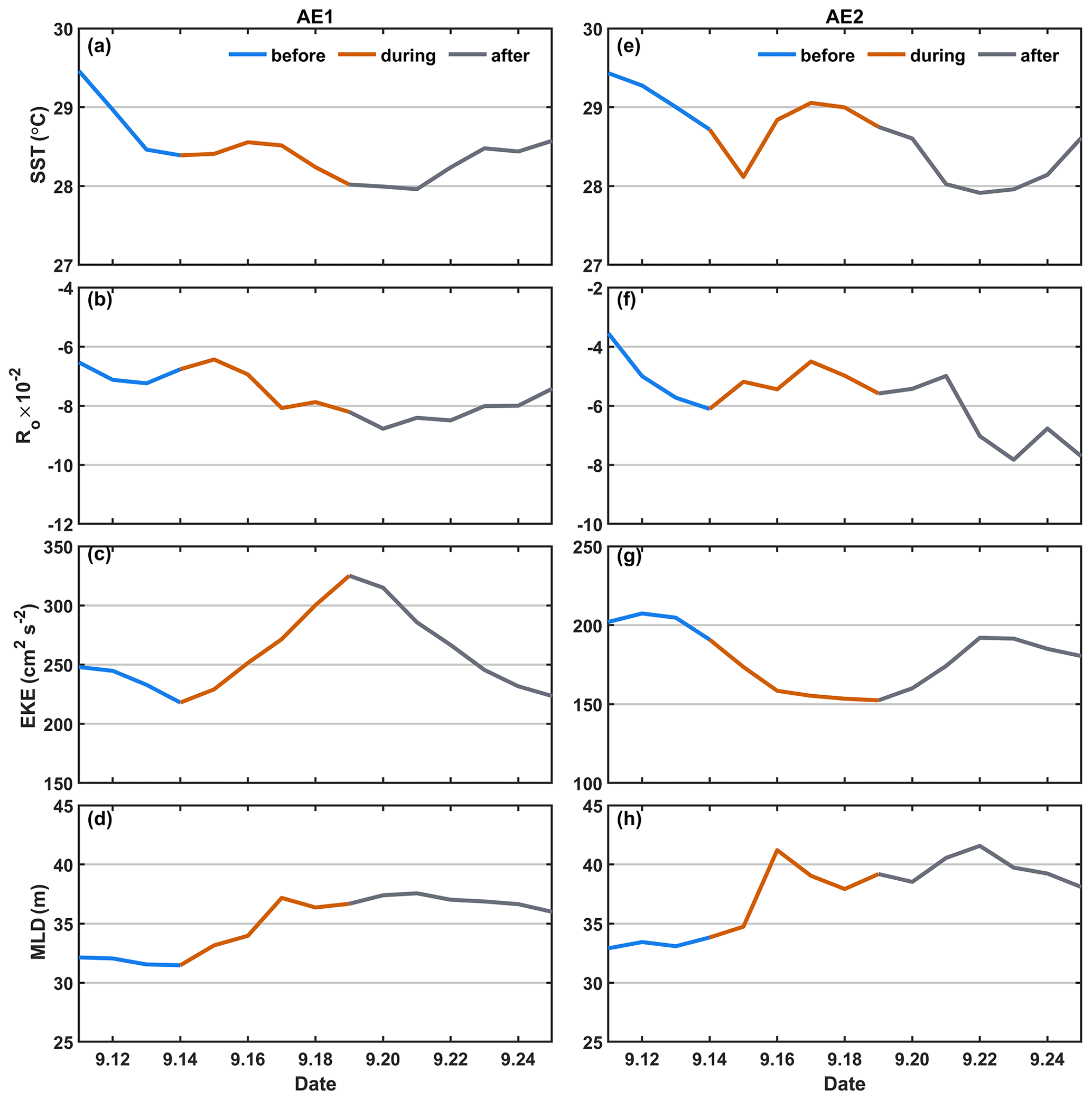
Figure 5 The time series of sea surface temperature (SST), Ro, eddy kinetic energy and mixed-layer depth (MLD) within the warm eddies' regions (solid black and dashed boxes in Fig. 4). The first column shows variables of AE1 and the second column variables of AE2.

We compare the Ro and EKE of AE1 and AE2 before, during and after the typhoon. Before being influenced by the typhoon, the warm eddy AE1 exhibited a more scattered distribution of negative Ro values due to its edge structure, and the EKE values at the eddy boundary were relatively high (Fig. 4d and g). As the typhoon passed through the eddy, the Ro and EKE of AE1 increased. On 19 September, the average Ro within AE1 reached a value of $-\mathrm{8.2}\times {\mathrm{10}}^{-\mathrm{2}}$; at the same time, the average EKE increased to its maximum value of 325.0 cm² s⁻². The variation trend of Ro and EKE within the eddy was consistent, increasing from the passage of the typhoon and starting to recover on 20 September (Fig. 5b and c). This indicates that although the area of the warm eddy AE1 decreased under the influence of the typhoon, its intensity increased. On the other hand, for warm eddy AE2, both Ro and EKE decreased after the typhoon passage, with Ro decreasing to $-\mathrm{4.5}\times {\mathrm{10}}^{-\mathrm{2}}$ on 17 September and EKE decreasing to 152.0 cm² s⁻² on 19 September, followed by a recovery (Fig. 5f and g). Unlike AE1, AE2 weakened in intensity under the influence of the typhoon.

During the passage of the typhoon, wind-stress-driven mixing enhancement and an increase in vertical shear resulted in a deepening of the MLD, which further strengthened the mixing between the deep cold water and the upper warm water (Shay and Jaimes, 2009). To avoid a large part of the strong diurnal cycle in the top few meters of the ocean, 10 m is set as the reference depth (De Boyer Montégut, 2004). A 0.5 °C threshold difference from 10 m depth is calculated and defined as the MLD (Thompson and Tkalich, 2014). Prior to the influence of Typhoon Kalmaegi, the MLD in the AE1 and AE2 regions was deeper (Fig. 4j), with average MLDs of 32 and 33 m, respectively. Starting from 14 September, the MLDs were influenced by Typhoon Kalmaegi, with the MLD of AE1 deepening to 37 m and that of AE2 increasing to 41 m, representing a deepening of 5 and 8 m, respectively (Fig. 5d and h).

Overall, Typhoon Kalmaegi likely had distinct impacts on the two warm eddies. Despite both AE1 and AE2 experiencing a decrease in their respective areas by approximately one-third, accompanied by deepening of the MLD, the amplitude of the SLA within AE1 increased by 1.3 cm, whereas AE2 witnessed a decrease of about 3.1 cm in its amplitude. Furthermore, the SST, Rossby number and EKE within AE1 and AE2 exhibited contrasting patterns.

3.2 Upper-ocean vertical thermal and salinity structure of eddies

We conducted further analysis on the vertical temperature and salinity structure of the warm eddies AE1 and AE2 before and after Typhoon Kalmaegi using GLORYS12V1 data. During the typhoon's passage on 15 September, the temperature above the MLD within AE1 increased by approximately 0.1 °C, while the salinity decreased by 0.02 psu (Fig. 6). Below the MLD, the temperature showed a significant increase, reaching a maximum temperature rise of 1.3 °C. Correspondingly, the salinity below the MLD exhibited a decrease of 0.05 psu. Vertical temperature on Kalmaegi's arrival day showed a warm pattern from the surface to 200 m, with the salinity showing “fresher–saltier” pattern. These changes led to a deepening of isopycnals by 15 m and a decrease in buoyancy frequency N² (Fig. 7a and b), indicating convergence and downwelling within the center of the warm eddy AE1. The near-inertial waves propagated downward from the surface to 200 m during this period (Zhang et al., 2016). The transfer of energy from anticyclonic eddy to near-inertial waves was the main reason for the downward propagation and long persistence of near-inertial energy (Chen et al., 2023).

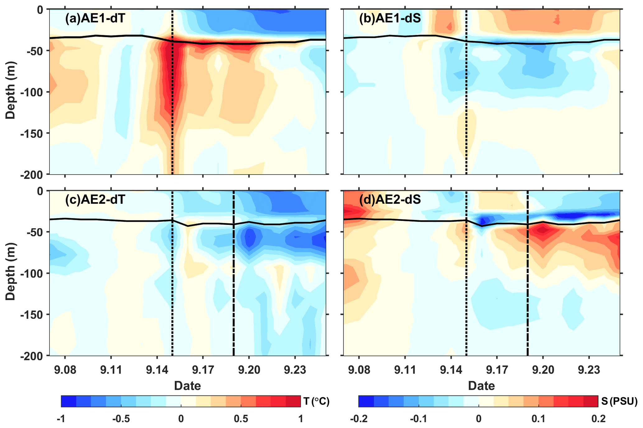
Figure 6 The time series of vertical temperature and salinity anomalies in the center of AE1 (a, b) and AE2 (c, d). The anomalies were calculated relative to the average value of 10–13 September. The dotted vertical black line indicates Typhoon Kalmaegi's passage, while the dashed vertical black line represents the passage of Tropical Storm Fung-wong. The solid black line is the MLD.

Figure 7 The same as Fig. 6 but for density and buoyancy frequency (N²).

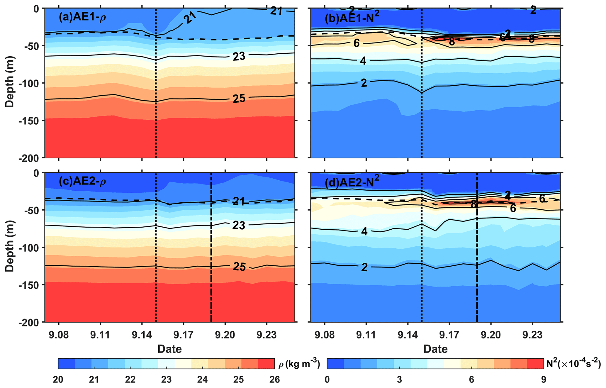
After 15 September, the temperature above the MLD decreased, and the salinity showed an increase (Fig. 6a and b), resulting in the uplift of the 1021 kg m⁻³ isopycnal to the sea surface (Fig. 7a and b). The subsurface warming and salinity reduction gradually weakened after Typhoon Kalmaegi but persisted for about a week after the typhoon's passage until 22 September. During this period, vertical temperature pattern became “cool–warm” at the center of AE1, and the salinity distribution pattern became “saltier–fresher–saltier”. This persistence can be attributed to the intensified stratification around the MLD, with N² around $\mathrm{9.0}\times {\mathrm{10}}^{-\mathrm{4}}$ s⁻² (Fig. 7b). The increased stability inhibited vertical mixing, restrained the exchange of heat and salinity, and led to smoother density gradients above the MLD (Fig. 7a).

The vertical temperature and salinity structure of AE2 exhibited an opposite trend. During the typhoon passage on 15 September, AE2 also experienced a cooling trend of 0.2 °C, with a decrease in salinity of 0.04 psu above the MLD. Below the MLD, the temperature showed a consistent decrease, with a change of less than 0.5 °C within the subsurface. Correspondingly, the salinity exhibited an increase of approximately 0.08 psu (Fig. 6c and d). The slightly upward shift of the isopycnals (Fig. 7c) suggests the possibility of cold-water upwelling induced by the suction effect of the typhoon. The temperature decreases and salinity increases below the MLD were primarily driven by upwelling.

Furthermore, when the Tropical Storm Fung-wong passed through AE2 on 19 September (dashed line in Fig. 6c and d), the decreasing trend of subsurface temperature became more pronounced and the subsurface salinity exhibited a significant increase. AE2 is more significantly influenced by Tropical Storm Fung-wong. It presents stable stratification with N² around $\mathrm{8.4}\times {\mathrm{10}}^{-\mathrm{4}}$ s⁻² at a depth of 42 m, creating a barrier layer that prevents the intrusion of high-salinity cold water from the lower layers into the mixed layer (Yan et al., 2017).

3.3 Comparison of the response between eddy and non-eddy areas

To investigate the contrasting response of warm eddies and the non-eddy background to Typhoon Kalmaegi, we conduct a comparative analysis of vertical temperature and salinity profiles in these two areas. Unfortunately, there are no Argo data from around AE1; therefore, we examine data from Argo 2901469, which was located within AE2 during the period from 11 to 19 September. The temperature and salinity data from Station 5 are considered to be the background, with Station 5 located at a distance of 246 km from AE2's center on 15 September (Fig. 1). These profiles are categorized into three periods: pre-typhoon (11 September), during-typhoon (15 September) and post-typhoon (19 September) stages.

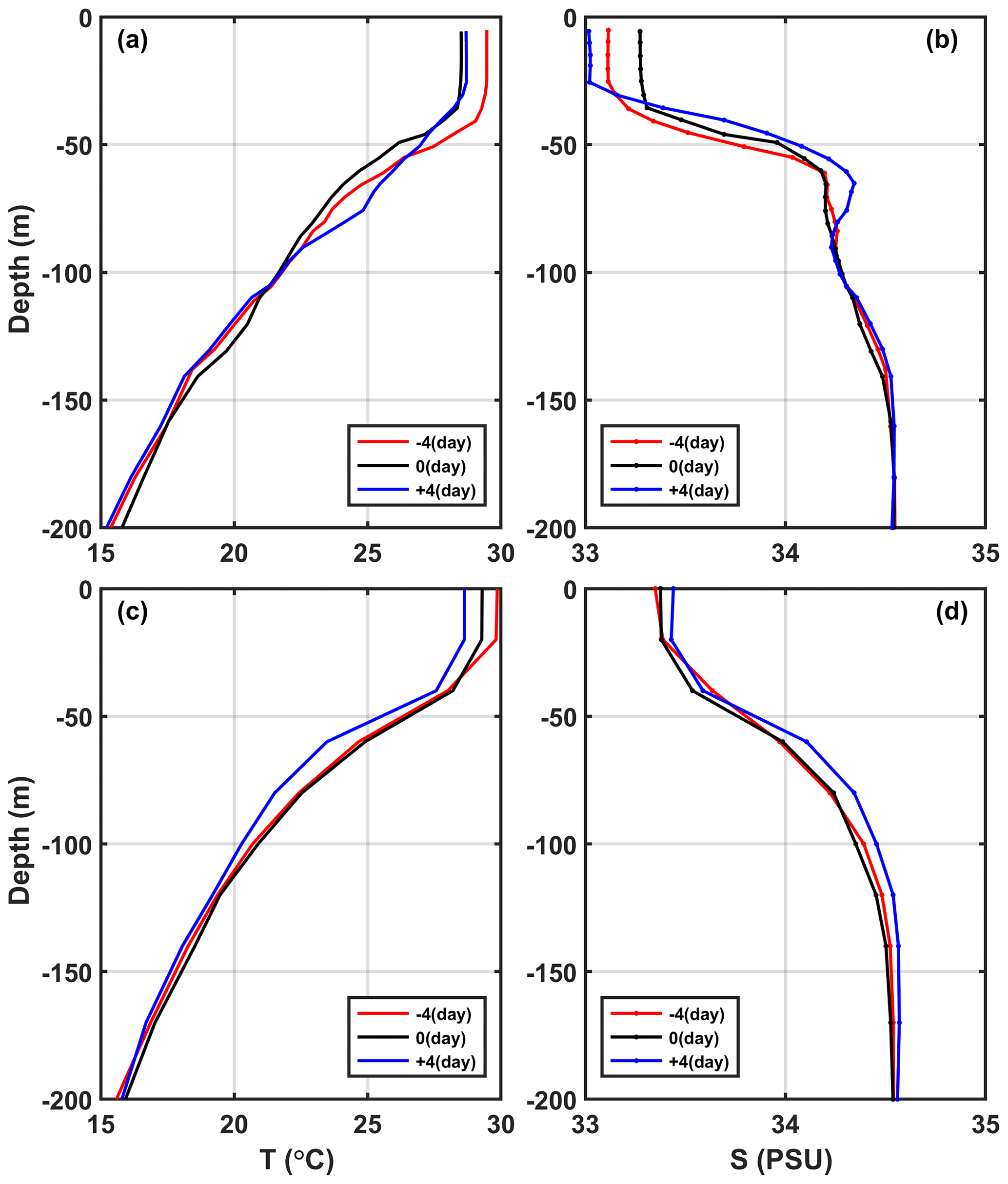
Figure 8 (a, b) The vertical profiles of temperature and salt inside the eddy (Argo 2901469). (c, d) The vertical profiles of temperature and salt outside the eddy (Station 5). The red, black and blue lines represent pre-typhoon, during-typhoon and post-typhoon stages.

At depths above 40 m, both the inside and the outside of AE2 experienced a decrease in temperature, with a cooling of less than −1.0 °C. On 19 September, 4 d after the typhoon passage, the cooling persisted inside and outside the eddy, with the cooling being more pronounced outside AE2, showing a decrease of 1.2 °C (Fig. 8c). The salinity within AE2 initially increased by 0.15 psu from the pre-typhoon stage to the during-typhoon stage and then decreased by 0.09 psu after the typhoon passage (Fig. 8d). While the salinity at Station 5 showed a similar pattern in the pre-typhoon and during-typhoon stages, it increased by 0.05 psu after the typhoon. Two possible processes can explain the difference in salinity trends inside and outside AE2. First, during the pre-typhoon to typhoon stage, the entrainment within AE2 may have brought the subsurface water, which is saltier, up to the surface, resulting in an increase in salinity. The second process is related to the typhoon-induced precipitation after the typhoon passage, which led to a decrease in salinity. Strong stratification contributed to the persistence of saltier subsurface water, while at Station 5, the increase in salinity was relatively minor.

On 15 September, the subsurface layer at 45 to 100 m was affected by the cold upwelling, which was caused by the typhoon, resulting in a cooling and increased salinity within AE2. As the forcing of Typhoon Kalmaegi diminished, the upper layer of seawater began to mix, and warm surface water was transported to the subsurface layer. A warming phenomenon occurred 4 d later, with the maximum warm anomaly of 1.2 °C observed at a depth of 75 m (Fig. 8a). The mixing effect outside the eddy was not significant, resulting in a slight subsurface warming of approximately 0.2 °C and no significant changes in salinity. However, on 19 September, a maximum cold anomaly of −1.2 °C was observed at a depth of 60 m, corresponding to the maximum salinity anomaly of 0.13 psu (Fig. 8c and d). Below 100 m, AE2 experienced a temperature increase of 0.5 °C and a slight decrease in salinity of 0.04 psu. On 19 September, the temperature and salinity within AE2 showed little change. However, outside the eddy, a different response was observed. On 19 September, a cooling trend was observed throughout the water column, within a range of 0.2 °C, accompanied by a noticeable increase in salinity (Fig. 8c and d), within a range of 0.06 psu. This indicates that the typhoon caused a significant upwelling outside the eddy region.

Based on Argo profiles and Station 5 data, the upper ocean above 200 m inside and outside AE2 responded differently to the forcing of the typhoon. In the upper layer (0–40 m), cooling was observed both inside and outside the eddy, and it lasted longer. In the subsurface layer (45–100 m), after the passage of the typhoon (19 September), there was a strong cooling outside the eddy, while warming occurred within AE2. Zhang (2022) points out that the sea temperature anomalies mainly depend on the combined effects of mixing and vertical advection (cold suction). Mixing causes surface cooling and subsurface warming, while upwelling (downwelling) leads to cooling (warming) of the entire upper ocean. The temperature anomaly in the subsurface layer depends on the relative strength of mixing and vertical advection, with cold anomalies dominating when upwelling is strong and downwelling amplifying the warming anomalies caused by mixing. Therefore, due to the strong influence of upwelling outside the eddy, the temperature profile of the entire water column shifted upward, resulting in cooling of the entire upper ocean. On the other hand, influenced by the downwelling associated with the warm eddy itself, a warming anomaly of 1.2 °C was observed in the subsurface layer. Compared to region AE2, the cold suction effect caused by Typhoon Kalmaegi was still evident in the non-eddy area.

In the following sections, we delve into the underlying reasons behind these different responses of AE1 and AE2 to Typhoon Kalmaegi.

4 Discussion

TCs influence mesoscale eddies through the baroclinic geostrophic response (Lu et al., 2020). The width of this response is generally constrained within the TC orbit, with the transverse diameter length represented as (Lu and Shang, 2024)

$$\begin{array}{}\text{(10)}& L_{\mathrm{h}}=L_{\mathrm{d}}+R_{\text{max}}.\end{array}$$

Here, L_d is the first mode of the Rossby deformation radius and R_max denotes the maximum wind radius. $L_{\mathrm{d}}=\frac{C}{f}$, the phase speed of the first baroclinic mode c was obtained using the method in Jaimes and Shay (2009). Therefore, the width of Typhoon Kalmaegi-induced baroclinic geostrophic response was in the range of 92 km (Fig. 3). Essentially, these geostrophic effects are caused by wind stress curl, and the wind stress curl injects disturbance into the ocean through upwelling and downwelling. Most of the positive wind stress curl exists within R_max, leading to strong upwelling, while the weak negative wind stress curl occurs outside R_max, resulting in weak subsidence caused by TCs that exist outside the upwelling area (Lu et al., 2020; Lu and Shang, 2024). Typhoon Kalmaegi strengthened after passing through the warm-ocean characteristics of AE2, causing a reduction in R_max. When passing AE1, R_max was 37 km. Notably, the center of AE1 was located outside R_max (Fig. 3). Hence, the hypothesis presented here suggests that the observed intensification of AE1 on the left side of the typhoon track is more likely attributed to the negative wind stress curl generated outside R_max, thereby driving the enhancement of downwelling in the pre-existing anticyclonic feature in the ocean.

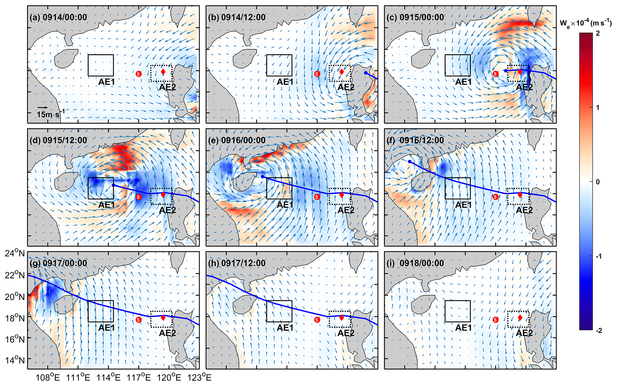
Figure 9 Ekman pumping velocity (EPV) from 14 September to 18 September (a–i). The color represents EPV; the solid blue line is the path of Kalmaegi; and the red dot and diamond are the positions of Station 5 and Argo 2901469, respectively, on 15 September.

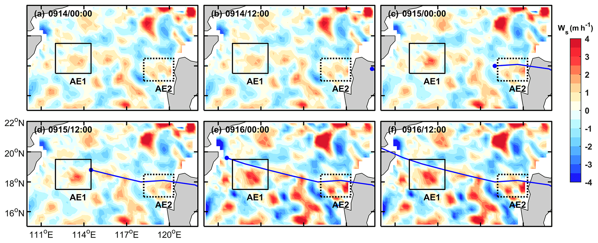
Figure 10 TC-driven pumping velocity (W_s) from 14 September to 16 September (a–f). The color represents W_s, and the solid blue line is the path of Kalmaegi. Negative and positive values are for upwelling and downwelling regimes, respectively.

EPV was very small before the typhoon, measuring less than $\mathrm{0.5}\times {\mathrm{10}}^{-\mathrm{5}}$ m s⁻¹ in both AE1 and AE2. However, during 15–16 September (Fig. 9c–f), when the typhoon crossed the NSCS, EPV underwent significant changes. Its absolute value increased to over $\mathrm{1.5}\times {\mathrm{10}}^{-\mathrm{4}}$ m s⁻¹ within both AE1 and AE2. AE1 consistently exhibits a predominantly negative EPV during most of this period. Consequently, during Typhoon Kalmaegi, the negative EPV facilitated downwelling and convergence (Jaimes and Shay, 2015), leading to a warmer and fresher subsurface layer in AE1 (Fig. 6a and b). On the other hand, AE2 displayed a more fluctuating pattern. It was positive on 14 September, showing both positive and negative values at 00:00 UTC on 15 September; remained mainly negative from 15 to 16 September; and eventually returned to positive, reflecting a continuously fluctuating process. The positive EPV in AE2 contributed to the influx of colder subsurface water into the upper layers, resulting in surface and subsurface water cooling and an increase in salinity in the subsurface (Fig. 6c and d).

Considering the influence of the background flow field, the pumping rate W is not only related to the wind stress curl (undisturbed Ekman pumping), but also related to the curl of background geostrophic flow (nonlinear Ekman pumping). Therefore, in order to describe the response of upwelling and downwelling more accurately, a parametric TC-driven pumping velocity scale (Jaimes and Shay, 2015),

$$\begin{array}{}\text{(11)}& W_{\mathrm{s}}=W_{\mathrm{E}}-\mathit{Ro}\mathit{\delta }\left(U_{\mathrm{h}}+U_{\text{OML}},\right)\end{array}$$

is derived from the time-dependent vorticity balance in the ocean mixed layer. Here W_E calculated by Eq. (8); Ro is calculated using Eq. (3); the aspect ratio is calculated by $\mathit{\delta }=\frac{h}{R_{\text{max}}}$, where h represents oceanic mixed-layer thickness; U_h denotes the translation speed; and oceanic mixed-layer Ekman drift is calculated by $U_{\text{OML}}=\frac{\mathit{\tau }{R}_{\text{max}}}{\mathit{\rho }h{U}_{\mathrm{h}}}$. The vertical velocity W_s calculated by Eq. (11) is presented in Fig. 10. When Typhoon Kalmaegi passed through AE1, the W_s in AE1 obviously increased, while AE2 experienced minimal change.

Starting from 15 September, a significant positive sea level anomaly (SLA) to the west of 113.5° E becomes evident, intensifying and reaching its maximum on 20 September (Fig. 11a). This strengthening aligns with the increase in the amplitude of the warm core of AE1. A comparison with the wind stress curl anomaly (Fig. 11b) reveals that between 15 and 16 September, as Typhoon Kalmaegi moved over the section at 18.2° N, specifically to the west of 113.5° E, it exhibited strong negative wind stress curl anomalies, with a maximum intensity of $-\mathrm{3}\times {\mathrm{10}}^{-\mathrm{6}}$ N m⁻³. The combined influence of negative wind stress curl and eddy strengthening enhanced the downwelling and induced negative vorticity in AE1, leading to its intensification (Fig. 4b and c), as indicated by the enhanced positive SLA (Fig. 11a). Conversely, the region to the east of 113.5° E along the section exhibited negative SLAs. This weakening is consistent with the previous observations of the intensified warm core and decreased eddy area.

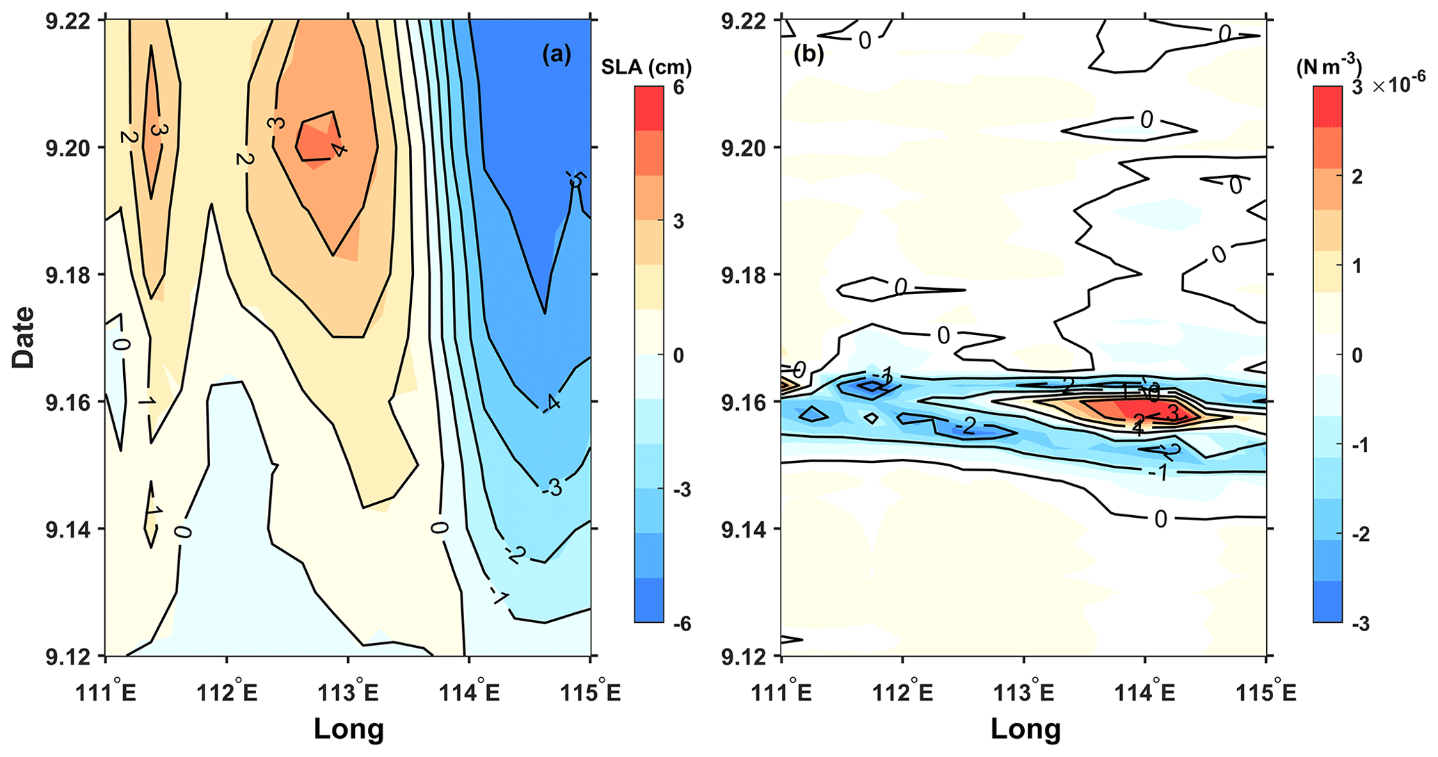
Figure 11 The time–longitude plots of the (a) SLA (cm) and (b) wind stress curl (N m⁻³) anomaly at the central section of AE1 (18.2° N). The anomalies were calculated relative to the average value of 10–13 September.

Figure 12 The same as Fig. 11 but for AE2 (17.9° N).

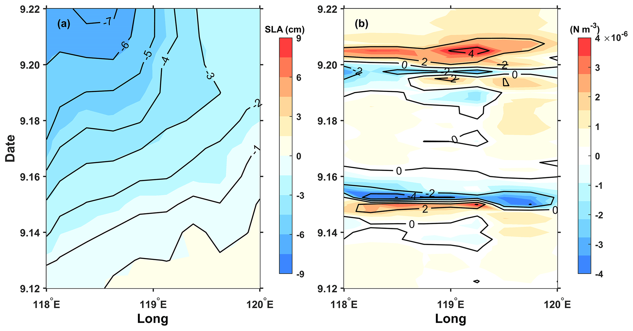
The response of AE2 differs from that of AE1 mainly because AE2 was quite near Typhoon Kalmaegi's track. As the typhoon passed through AE2, R_max was 46 km. AE2 was merely 26 km away from the typhoon center (Fig. 3). The significantly positive wind stress curl at the typhoon center induced upwelling and positive vorticity downward into the eddy (Huang and Wang, 2022) and noticeably weakened the eddy, corresponding to the decrease in the SLA (Fig. 12a). Furthermore, based on the meridional isotherm profiles of the eddy center on three dates, it can be observed that during the passage of Typhoon Kalmaegi (15 September), the isotherms in the AE1 region exhibited significant subsidence (Fig. 13a), while in the AE2 region, the isotherms showed uplift (Fig. 13b). This result aligns with the earlier observation that the convergence and subsidence within the warm eddy AE1 were enhanced by the influence of the wind stress curl induced by the typhoon, while the intensity of AE2 was weakened.

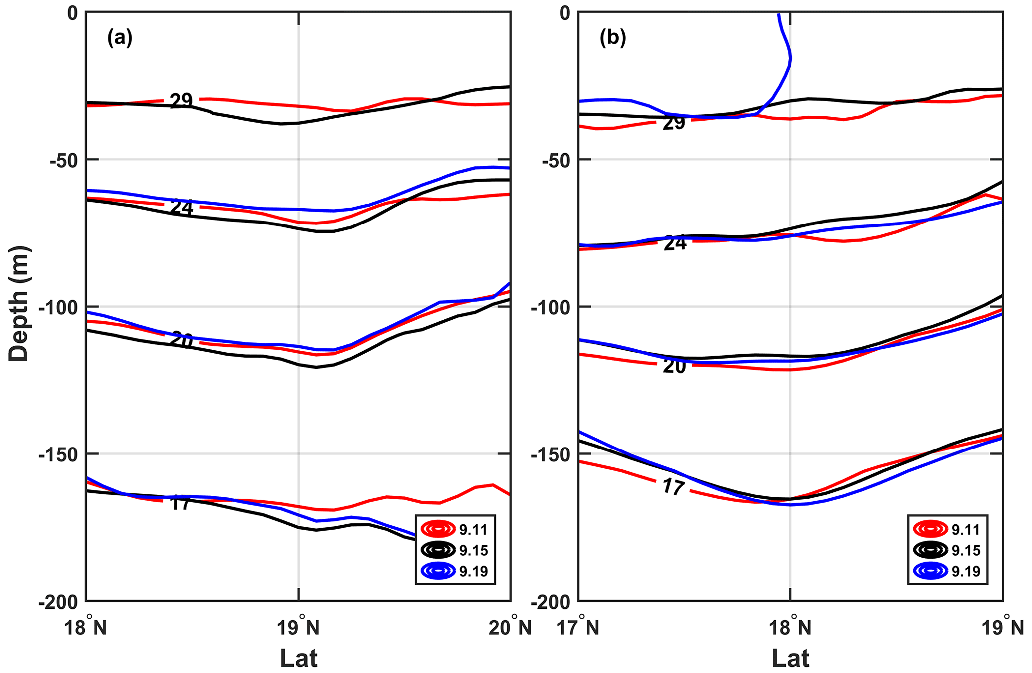
Figure 13 The meridional isotherm profiles of AE1 (a) and AE2 (b) before (11 September), during (15 September) and after (19 September) Typhoon Kalmaegi.

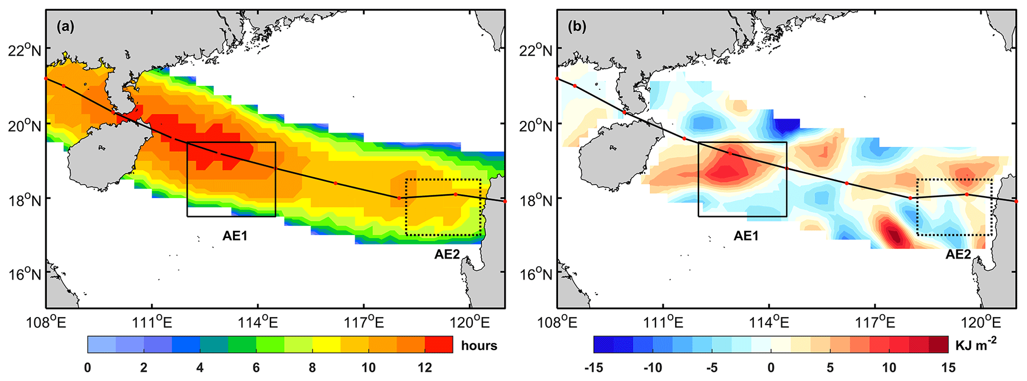
Figure 14 (a) The forcing time (unit: h) of the typhoon; (b) the input work (unit: kJ m⁻²) of the typhoon on the current.

From the above, the relative position of eddies and the typhoon can influence the response of the eddies (Lu et al., 2020). The warm eddy AE1, located on the left side of the typhoon track, was not weakened by the strong cold suction effect caused by Typhoon Kalmaegi. Instead, it was strengthened due to the stronger negative wind stress curl generated by the typhoon.

To understand the work done by Typhoon Kalmaegi on the eddies in the ocean, we estimate the total work input into the ocean current u_c using the previously calculated wind stress (Liu et al., 2017):

$$\begin{array}{}\text{(12)}& W=\int \mathit{\tau }\cdot {\mathit{u}}_{\mathbf{c}}\mathrm{d}t.\end{array}$$

Here, we select the region near the typhoon track where the wind speed exceeds 17 m s⁻¹ as the typhoon forcing region to know the energy input by the typhoon to the warm eddy (Sun et al., 2010). The forcing duration over the ocean in the typhoon-affected region and the work done by the typhoon on the surface current are shown in Fig. 14. When the angle between the wind and the ocean current is acute, the typhoon does positive work on the ocean current. Conversely, when the angle is obtuse, the typhoon does negative work on the ocean current. It is evident that the region with the maximum forcing duration by the typhoon acting on AE1 corresponds to the area where the typhoon clearly does positive work on the ocean current, accumulating a total of work done exceeding 8 kJ m⁻². This acceleration of the flow velocity in the eddy results in convergence within the eddy and an increase in the SLA, leading to the strengthening of AE1. On the other hand, the forcing duration by the typhoon on AE2 is smaller, and the typhoon does negative work on the ocean current in most areas, with a cumulative work done within −5 kJ m⁻², causing the flow velocity within AE2 to decelerate.

5 Summary

Based on multi-satellite observations, in situ measurements and numerical model data, we have gained valuable insights into the response of the warm eddies AE1 and AE2 in the northern South China Sea to Typhoon Kalmaegi. Both horizontally and vertically, these eddies displayed distinct differences. Horizontally, AE1 was located outside the R_max of typhoon. Its amplitude, Ro and EKE strengthened after the passage of the typhoon. In contrast, AE2 weakened and was positioned within the R_max of the typhoon. Vertically, during the typhoon's passage, AE1 experienced intensified converging subsidence flow at its center, leading to an increase in temperature and a decrease in salinity above 150 m. This response was more pronounced below the MLD (1.3 °C) and persisted for about a week after the typhoon. On the other hand, AE2 exhibited cooling above the MLD, accompanied by a decrease in salinity, as well as a subsurface temperature drop and salinity increase due to the upwelling of cold water caused by the typhoon's suction effect. Additionally, it can be seen that the non-eddy region also experienced significant cooling, with a prominent cooling center observed at a depth of 60 m (−1.2 °C).

Further analysis reveals that the different responses of the warm eddies can be attributed to factors such as wind stress curl distribution, which were influenced by the relative position of the warm eddies and the typhoon track. The wind stress curl induced by the typhoon played a crucial role in shaping the response of the warm eddies. AE1, located outside the R_max of the typhoon, was subjected to a negative wind stress curl which generated a potential vorticity perturbation inside the eddy. W_s was enhanced by wind stress curl and quasi-geostrophic adjustment of the perturbed eddies. Therefore, the downwelling within AE1 is obvious and contributed to its increased strength. In contrast, AE2, positioned directly below the typhoon's track, experienced a shorter forcing duration and weakened due to the strong positive wind stress curl at the typhoon's center. Furthermore, the absolute value of EPV increased in both warm eddies during the typhoon's passage but with differing impacts. Under typhoon conditions, the combined action of wind Ekman pumping and eddy Ekman pumping made the same polar eddies respond differently to the typhoon at different positions.

Numerous prior studies exploring the interaction between TCs and eddies have predominantly drawn generalized conclusions, such as the weakening (strengthening) effect of cold (warm) eddies. However, our study takes a different approach. We aim to illustrate that even when TCs encounter eddies of the same polarity, the response of these eddies to TCs exhibits variations. This nuanced response is intricately linked to factors including the relative position of the eddies and the TCs, the eddies' intensity, and the background current. This is discussed for the first time in relation to the South China Sea. By analyzing wind stress curl distribution, EPV, buoyancy frequency, and the relative position between the eddies and the typhoon's track, this case study provides a more nuanced understanding of the mechanisms driving these different eddy–typhoon interactions in the northern South China Sea. Moreover, it will further improve the accuracy of TC forecasts and enhance the simulation capabilities of air–sea coupled models.