Influence of stratification and wind forcing on the dynamics of Lagrangian residual velocity in a periodically stratified estuary

Wind and stratification play pivotal roles in shaping the structure of the Lagrangian residual velocity (LRV). However, the intricate dynamics by which wind and stratification modify the LRV remain poorly studied. This study derives numerical solutions of LRV components and eddy viscosity subcomponents to elucidate the dynamics within the periodically stratified Pearl River estuary. The vertical shear cross-estuary LRV (u_L) is principally governed by the interplay among the eddy viscosity component (u_Ltu), the barotropic component (u_Lba), and the baroclinic component (u_Lgr) under stratified conditions. During neap tides, southwesterly winds notably impact u_L by escalating u_Ltu by an order of magnitude within the upper layer. This transforms the eastward flow dominated by u_Ltu under wind influence into a westward flow dominated by u_Lba in upper shoal regions without wind forcing. The along-estuary LRV exhibits a gravitational circulation characterized by upper-layer outflow engendered by a barotropic component (v_Lba) and lower-layer inflow predominantly driven by a baroclinic component (v_Lgr). The presence of southwesterly winds suppresses along-estuary gravitational circulation by diminishing the magnitude of v_Lba and v_Lgr. The contributions of v_Lba and v_Lgr are approximately equal, while the ratio between u_Lba and u_Lgr (u_Ltu) fluctuates within the range of 1 to 2 in stratified waters. Under unstratified conditions, LRV exhibits a lateral shear structure due to differing dominant components compared to stratified conditions. In stratified scenarios, the eddy viscosity component of LRV is predominantly governed by the turbulent mean component, while it succumbs to the influence of the tidal straining component in unstratified waters.

1 Introduction

Tidal currents are the principal movement in shallow seas and estuaries. However, tidal oscillations are not the predominant factor regarding the long-term transport of mass, such as pollutants, sediments, nutrients, and suspended materials. Instead, residual current, which remains after filtering out tidal movements, plays a crucial role in long-term mass transport. Therefore, unveiling the dynamic mechanisms governing the structure and magnitude of the residual current becomes particularly important for a correct understanding of the circulation and long-term mass transport in shallow seas and estuaries.

Pritchard (1952) proposed a conceptual model of estuarine circulation characterized by a two-layer structure, drawing from extensive observations. A subsequent study by Pritchard (1956) emphasized the crucial role of the horizontal density gradient as the primary driving force for estuarine circulation. Subsequently, the theory of estuarine gravitational circulation was developed, assuming a constant eddy viscosity (Hansen and Rattray, 1965). Nevertheless, it is imperative to acknowledge that estuarine circulation is influenced not solely by density gradients but also by factors such as wind, tides, and other dynamic forces. These external factors possess the ability to modify or even reverse the structure of gravitational circulation within estuaries.

To remove the tidal signal, early researchers such as Abbott (1960) utilized a straightforward method by averaging current velocities over one or several tidal periods at a specific location to calculate the Eulerian residual velocity (ERV). Several studies have highlighted the impact of tidal straining on Eulerian residual velocity (ERV) (e.g., Becherer et al., 2011; Burchard et al., 2014, 2023). Jay and Musiak (1994) found the ERV induced by tidal straining is comparable to gravitational circulation. Additionally, tidal straining contributes twice as much to the ERV as gravitational circulation without consideration of river runoff (Burchard and Hetland, 2010). The flow induced by tidal straining varies in estuaries with different stratified conditions. When the horizontal density gradient is small, tidal straining dominates the structure of the ERV (Burchard et al., 2011). Cheng et al. (2011) showed that tidal straining induces a typical two-layer circulation in weakly stratified estuaries, while the circulation exhibits a vertical three-layer structure with inflow in the upper and lower layer and outflow in the middle layer in partially and heavily stratified estuaries. As stratification intensifies, the ratio of flow induced by tidal straining to gravitational circulation decreases. In a weakly stratified short estuary, tidal straining plays a secondary role in ERV compared to gravitational circulation (Wei et al., 2021). Geyer and MacCready (2014) indicated that the Eulerian mean method tends to overestimate the contribution of tidal straining. Therefore, it is more reasonable to analyze dynamical mechanisms for residual current from the perspective of the Lagrangian tidally averaged theory.

Wind, in conjunction with tides and density gradients, exerts a substantial influence on estuarine residual currents and stratification (Verspecht et al., 2009; Jongbloed et al., 2022). Its role in the generation of surface residual currents is underscored by the strong correlations observed between wind speeds and residual current velocities across both annual and seasonal timescales (Ren et al., 2022). Research on the Dongsha atoll revealed that the combined effects of wind and tide introduce more dynamic water exchange compared to tides alone (Chen, 2023). In the Bohai Sea area off Qinhuangdao, residual currents exhibit pronounced seasonal fluctuations, correlating notably with wind speeds at specific temporal lags (Zhang et al., 2023). Furthermore, the shift in wind-driven circulation is pivotal for mass transport within bays, with estuarine residual circulation superseding tidal pumping as the primary transport mechanism (Young et al., 2023). Burchard (2009) highlighted that upstream winds weaken stratification and reduce the magnitude of the ERV, whereas the downstream wind have the opposite effect. To quantify the destratification effect of upstream wind, Lange and Burchard (2019) introduced the Wedderburn number to analyze the relationship between upstream wind and density gradient. The wind is less inclined to affect the residual current with large Wedderburn numbers and may inhibit gravitational circulation, whereas the structure of ERV reverses with small Wedderburn numbers. Wind plays a pivotal role in modulating classical gravitational circulation, most notably reversing surface outflow during winter. In contrast, northward winds in spring enhance stratification and augment the pressure-gradient-driven flow (Soto-Riquelme et al., 2023).

The Eulerian mean method is a prevalent approach for examining estuarine dynamics; however, specific terms within its momentum and mass transport equations remain ambiguous in their physical interpretations (Ianniello, 1977; Feng et al., 1984). Lamb (1993) posited that any flow field must adhere to the mass conservation principle. Zimmerman (1979) defined Lagrangian residual velocity (LRV) as the net displacement of the water parcels over one or several tidal periods. Contextualizing this, the LRV, rooted in the intrinsic principles of physical motion, upholds material conservation and offers a precise portrayal of circulation dynamics in shallow marine environments (Feng, 1987; Jiang and Feng, 2014).

Lagrangian particle tracking methods play a pivotal role in studying mass transport and residence time (RT) across various coastal seas, estuaries, and bays. Specific water mass transport patterns are discerned in the Bohai Sea, revealing salient regional transport characteristics steered by LRV (Yu et al., 2023). The combined effects of residual transport velocity in the current and next seasons emerge as the predominant factor driving the RT's seasonal variation (Lin et al., 2022). Wind direction, wind speed, and density-gradient-induced circulation collectively regulate RT (Hewageegana et al., 2023). The reduction in cross-shore currents results in mass convergence and increases RT (Li et al., 2022). The water exchange and RT are mainly determined by the structure of the LRV (Jiang and Feng, 2014). RT predominantly represents an accumulative measure, primarily influenced by residual transport rather than immediate responses (Jiang, 2023). Convergence zones resulting from LRV efficiently establish consistent aggregation regions of buoyant material within the estuary rather than ERV (Kukulka and Chant, 2023). To gain an in-depth understanding of mass transport, extensive prior research has been dedicated to elucidating qualitative and quantitative evaluations of the determinants impacting the LRV's structure and magnitude. The influence of LRV in semi-closed estuaries and bays affected by tides has received attention from oceanographers (Winant, 2008; Jiang and Feng, 2011; Deng et al., 2019). Quan et al. (2014) employed a numerical model to investigate the impact of the ratio of tidal amplitude to water depth on LRV, and Jiang and Feng (2014) explored how the ratio of estuary length to wavelength affects LRV. Wang et al. (2010) examined the effects of wind, density gradient, and river runoff on LRV using a numerical model. However, this study aims to illustrate structural and magnitudinal variations in the total LRV under different factors without delving into the underlying dynamic mechanisms. Liu et al. (2021) demonstrated that the influence of wind and density gradients on LRV is closely associated with the initial tidal phase based on the momentum equations, but the specific contribution of each dynamic component to LRV remains poorly studied.

Jiang and Feng (2014) explored the dynamical mechanisms for the LRV, which leads to the assumptions of a constant eddy viscosity and linear bottom friction in the entire estuary. Subsequently, numerical models were utilized to study the contribution of tidal body force to LRV under a constant eddy viscosity, revealing that the Stokes drift component plays a dominant role (Cui et al., 2019). Chen et al. (2020) analyzed the contribution of each dynamical term to the LRV and found the Stokes drift component is the dominant component under the condition of the horizontally unvaried but depth-varying eddy viscosity. The above studies are all carried out under a temporally constant eddy viscosity. The impact of spatially varying eddy viscosity on LRV was examined in a narrow model, revealing that nonlinearity leads to a more complex LRV structure (Deng et al., 2017). However, these studies lack a quantitative analysis of the underlying dynamical mechanism. Sheng et al. (2022) demonstrated that the structure of LRV is primarily determined by the combined effects of the barotropic pressure gradient and tidal body force when only barotropic conditions are considered. Deng et al. (2022) further quantitatively analyzed the contributions of each driving force to LRV, considering both temporal and spatial variations in eddy viscosity under a constant density gradient. However, the roles of wind and stratification in LRV dynamics remain poorly studied.

The Pearl River, as the third largest river in China, encompasses a complex hydrodynamic environment. The Pearl River estuary (PRE) is a trumpet-like estuary characterized by two deep channels and shallow shoals. In recent years, researchers have increasingly focused on topics such as tidal currents, salinity intrusion, river plume dynamics, and residual current in the PRE (e.g., Gong et al., 2018; Pan et al., 2020; Wei et al., 2022). The estuary displays a typical two-layer circulation as observed in micro-tidal estuaries (Xue et al., 2001). Wang (2014) investigated the temporal and spatial variations in the ERV and analyzed its underlying dynamical mechanisms within the PRE. Lai et al. (2018) discussed the influence of tides and winds on the ERV and the associated dynamical processes using the Eulerian mean momentum equation. Additionally, the nonlinear advection term was identified as an important factor in the ERV within the PRE (Xu et al., 2021). An counterclockwise shift in summertime wind direction from 1979 to 2020 weakens cross-channel wind-driven transport and along-channel seaward flow, leading to increased stratification near the Modaomen Estuary (Hong et al., 2022). While Chu et al. (2022) explored the hydrodynamic processes and connectivity of the circulation within the estuary from a Lagrangian tidally averaged perspective, a detailed dynamical analysis was not provided. Few studies have focused on the LRV within the PRE, especially regarding its underlying dynamical mechanisms.

Analytical solutions regarding the dynamics of LRV are constrained to a temporally constant eddy viscosity, while numerical solutions of LRV's dynamic components disregard the influence of stratification and wind. Consequently, the impact of wind and stratification on LRV dynamics remains enigmatic. Numerical solutions for LRV components are derived to grasp the modifications induced by wind and stratification within each LRV component, ultimately leading to changes in the overall LRV. Furthermore, wind and stratification influence turbulent mixing, subsequently affecting the LRV driven by the eddy viscosity term. Although scholars have extensively examined tidal straining effects on estuarine circulation via the Eulerian mean theory, the analysis of turbulent influences from the Lagrangian mean theory perspective yields distinctions from the Eulerian approach. To illuminate the mechanisms underlying the eddy viscosity component of LRV, we begin by decomposing this component into four subcomponents. This study pursues two principal objectives: (1) to delve into the mechanisms by which wind and stratification modify LRV components and (2) to investigate the roles of wind and stratification in affecting the dominant contributing factors of the eddy viscosity component. This paper will provide valuable insights into the dynamic processes of longitudinal and lateral estuarine circulation based on Lagrangian mean theory under the influence of wind and stratification. These aspects have not been quantitatively assessed in previous studies. Additionally, the proposed decomposition theory of the eddy viscosity component offers a novel approach for analyzing the dominant mechanisms of turbulent components. This paper is structured as follows: Sect. 2 provides a delineation of model setup parameters, model validation, and LRV decomposition methods. Section 3 outlines the contribution of each component to the overall LRV and the contribution of each subcomponent to the total eddy viscosity component of LRV. The discussion and conclusions are presented in Sect. 4.

2 Theory and model description

2.1 The decomposition method

The LRV is decomposed into seven components, including the local acceleration component (u_Lac and v_Lac), horizontal nonlinear advection component (u_Ladh and v_Ladh), vertical nonlinear advection component (u_Ladv and v_Ladv), barotropic pressure gradient component (barotropic component; u_Lba and v_Lba), baroclinic pressure gradient component (baroclinic component; u_Lgr and v_Lgr), eddy viscosity component (u_Ltu and v_Ltu), and horizontal diffusion component (u_Lho and v_Lho). The detailed decomposition methods are shown in the Appendix. Deng et al. (2022) considered a temporally constant density gradient but neglected the effects of periodic stratification and wind forcing. In this paper, one of the primary objectives is to quantify the effects of wind and stratification on the dynamics of the different components of LRV.

Wind and stratification play roles in turbulent mixing, which subsequently impacts the fluctuations in eddy viscosity over a tidal period. This influence extends to the eddy viscosity component of LRV. To clarify the mechanisms underlying this eddy viscosity component, we decompose it into four subcomponents. We evaluate the distinct contributions of each subcomponent to the total eddy viscosity component, aiming to delve into the dominant dynamic mechanisms, which is another objective of our paper. The study derives the following decomposition methods:

$$\begin{array}{}\text{(1)}& {\displaystyle }\begin{array}{rl}-& 〈{\displaystyle \frac{\mathrm{1}}{D^{\mathrm{2}}}}{\displaystyle \frac{\partial }{\partial \mathit{\sigma }}}\left(v_h{\displaystyle \frac{\partial u}{\partial \mathit{\sigma }}}\right)〉/f=-〈{\displaystyle \frac{\mathrm{1}}{D^{\mathrm{2}}}}{\displaystyle \frac{\partial }{\partial \mathit{\sigma }}}\left(v_{h\mathrm{0}}{\displaystyle \frac{\partial u_{\mathrm{0}}}{\partial \mathit{\sigma }}}\right)〉/f\\ & -〈{\displaystyle \frac{\mathrm{1}}{D^{\mathrm{2}}}}{\displaystyle \frac{\partial }{\partial \mathit{\sigma }}}\left(v_{h\mathrm{0}}{\displaystyle \frac{\partial u_{\mathrm{1}}}{\partial \mathit{\sigma }}}\right)〉/f\\ & -〈{\displaystyle \frac{\mathrm{1}}{D^{\mathrm{2}}}}{\displaystyle \frac{\partial }{\partial \mathit{\sigma }}}\left(v_{h\mathrm{1}}{\displaystyle \frac{\partial u_{\mathrm{0}}}{\partial \mathit{\sigma }}}\right)〉/f-〈{\displaystyle \frac{\mathrm{1}}{D^{\mathrm{2}}}}{\displaystyle \frac{\partial }{\partial \mathit{\sigma }}}\left(v_{h\mathrm{1}}{\displaystyle \frac{\partial u_{\mathrm{1}}}{\partial \mathit{\sigma }}}\right)〉/f,\end{array}\text{(2)}& {\displaystyle }\begin{array}{rl}& 〈{\displaystyle \frac{\mathrm{1}}{D^{\mathrm{2}}}}{\displaystyle \frac{\partial }{\partial \mathit{\sigma }}}\left(v_h{\displaystyle \frac{\partial v}{\partial \mathit{\sigma }}}\right)〉/f=〈{\displaystyle \frac{\mathrm{1}}{D^{\mathrm{2}}}}{\displaystyle \frac{\partial }{\partial \mathit{\sigma }}}\left(v_{h\mathrm{0}}{\displaystyle \frac{\partial v_{\mathrm{0}}}{\partial \mathit{\sigma }}}\right)〉/f\\ & +〈{\displaystyle \frac{\mathrm{1}}{D^{\mathrm{2}}}}{\displaystyle \frac{\partial }{\partial \mathit{\sigma }}}\left(v_{h\mathrm{0}}{\displaystyle \frac{\partial v_{\mathrm{1}}}{\partial \mathit{\sigma }}}\right)〉/f+\\ & 〈{\displaystyle \frac{\mathrm{1}}{D^{\mathrm{2}}}}{\displaystyle \frac{\partial }{\partial \mathit{\sigma }}}\left(v_{h\mathrm{1}}{\displaystyle \frac{\partial v_{\mathrm{0}}}{\partial \mathit{\sigma }}}\right)〉/f+〈{\displaystyle \frac{\mathrm{1}}{D^{\mathrm{2}}}}{\displaystyle \frac{\partial }{\partial \mathit{\sigma }}}\left(v_{h\mathrm{1}}{\displaystyle \frac{\partial v_{\mathrm{1}}}{\partial \mathit{\sigma }}}\right)〉/f,\end{array}\end{array}$$

and

$$\begin{array}{}\text{(3)}& u=u_{\mathrm{0}}+u_{\mathrm{1}},v=v_{\mathrm{0}}+v_{\mathrm{1}},v_h=v_{h\mathrm{0}}+v_{h\mathrm{1}},\end{array}$$

where < > represents the Lagrangian-averaged operator; u and v are horizontal tidal currents; v_h is the eddy viscosity; u₁ and v₁ are tidal-averaged currents; and u₀ and v₀ are tidal periodic oscillation currents, which are referred to as the zero-order terms. These zero-order terms are equivalent in meaning to u^′ and v^′ as defined in prior studies (Burchard and Hetland, 2010; Burchard et al., 2011, 2014; Cheng, 2014). The terms u₁and v₁ correspond to the first-order terms and represent the tidal-averaged current. The v_h0 is tidal-averaged eddy viscosity, with the zero-order term with v_h1 representing the tidal periodic oscillation of the eddy viscosity as the first-order term. The D is time-varying depth, σ is the sigma coordinate, and f is the Coriolis parameter. Employing a first-order Taylor expansion, the approximation of $\mathrm{1}/D^{\mathrm{2}}$ is represented as $\mathrm{1}/H^{\mathrm{2}}-\mathrm{2}\mathit{\zeta }/H^{\mathrm{3}}$ (Cheng, 2014), where H signifies the mean depth and ζ corresponds to the sea surface elevation. Within the vast majority of the Pearl River Estuary, the ratio of ζ_max to H remains below 0.2 during neap tides, with an exception in nearshore areas, where ζ_max is the maximum of tidal elevations during a tidal period. The ratio during spring tides is slightly larger than that during neap tides. But whether during spring or neap tides, the terms associated with $\mathrm{1}/H^{\mathrm{2}}$ exhibit a close correspondence to those related to 1/D² in Eqs. (1) and (2) (not shown). The terms pertaining to $-\mathrm{2}\mathit{\zeta }/H^{\mathrm{3}}$ are sufficiently minor to be negligible. Consequently, considering D is approximately equivalent to H, further decomposition of D in the paper is not undertaken. The $\mathrm{-}\langle \frac{\mathrm{1}}{D^{\mathrm{2}}}\frac{\partial }{\partial \mathit{\sigma }}\left(v_{h\mathrm{0}}\frac{\partial u_{\mathrm{0}}}{\partial \mathit{\sigma }}\right)\rangle /f$ and $\langle \frac{\mathrm{1}}{D^{\mathrm{2}}}\frac{\partial }{\partial \mathit{\sigma }}\left(v_{h\mathrm{0}}\frac{\mathit{\delta }{v}_{\mathrm{0}}}{\partial \mathit{\sigma }}\right)\rangle /f$ represent the coupled component of the tidal-averaged eddy viscosity and velocity gradient oscillation (v_Lk0u0 and u_Lk0u0), the $-\langle \frac{\mathrm{1}}{D^{\mathrm{2}}}\frac{\partial }{\partial \mathit{\sigma }}\left(v_{h\mathrm{1}}\frac{\partial u_{\mathrm{0}}}{\partial \mathit{\sigma }}\right)\rangle /f$ and $\langle \frac{\mathrm{1}}{D^{\mathrm{2}}}\frac{\partial }{\partial \mathit{\sigma }}\left(v_{h\mathrm{1}}\frac{\partial v_{\mathrm{0}}}{\partial \mathit{\sigma }}\right)\rangle /f$ represent the tidal straining component (v_Lk1u0 and u_Lk1u0), the $-\langle \frac{\mathrm{1}}{D^{\mathrm{2}}}\frac{\partial }{\partial \mathit{\sigma }}\left(v_{h\mathrm{0}}\frac{\partial u_{\mathrm{1}}}{\partial \mathit{\sigma }}\right)\rangle /f$ and $\langle \frac{\mathrm{1}}{D^{\mathrm{2}}}\frac{\partial }{\partial \mathit{\sigma }}\left(v_{h\mathrm{0}}\frac{\partial v_{\mathrm{1}}}{\partial \mathit{\sigma }}\right)\rangle /f$ represent the turbulent mean component (v_Lk0u1 and u_Lk0u1), and the $-\langle \frac{\mathrm{1}}{D^{\mathrm{2}}}\frac{\partial }{\partial \mathit{\sigma }}\left(v_{h\mathrm{1}}\frac{\partial u_{\mathrm{1}}}{\partial \mathit{\sigma }}\right)\rangle /f$ and $\langle \frac{\mathrm{1}}{D^{\mathrm{2}}}\frac{\partial }{\partial \mathit{\sigma }}\left(v_{h\mathrm{1}}\frac{\partial v_{\mathrm{1}}}{\partial \mathit{\sigma }}\right)\rangle /f$ represent the coupled component of eddy viscosity oscillation and the tidal-averaged velocity gradient (v_Lk1u1 and u_Lk1u1).

2.2 Model configuration and experiments

This study employs the Finite Volume Community Ocean Model (FVCOM; Chen et al., 2006) to simulate the dynamic response of LRV to wind and stratification in the PRE. FVCOM is a three-dimensional primitive equation community ocean model (Chen et al., 2003) that utilizes a finite-volume approach, accounting for a free surface and employing prognostic techniques. The model consists of unstructured triangular cells and employs terrain-following vertical coordinates, allowing for a better fit of the irregular coastline and complex topography present in the estuary.

The model domain, covering the PRE and adjacent coastal regions, is depicted in Fig. 1, spanning from 111.5 to 116.5° E and 20 to 23° N. The open boundary is situated in the northern South China Sea. Unidirectional grid nesting is implemented to enhance solution algorithms. The coarse grid consists of 8040 nodes and 15 093 triangular elements. The spatial resolution of the horizontal grids varies across the entire region, ranging from 1 to 10 km. Specifically, a resolution of 1 km is employed within the PRE, 2.0–5.0 km off the Guangdong coast, and 10 km near the open boundary (Fig. 1a). On the other hand, the fine grid, consisting of 45 368 nodes and 87 179 triangular elements, is configured based on the settings from previous studies (e.g., Lai et al., 2018; Geyer et al., 2020; Xu et al., 2021). The spatial resolution of the fine grids within the region also varies, ranging from 0.1 to 2.0 km. More specifically, a resolution of 0.1 km is utilized within the PRE, 0.1–1.0 km off the Guangdong coast, and 2.0 km close to the open boundary (Fig. 1b). In the vertical direction, the model employs 14 uniformly assigned sigma levels.

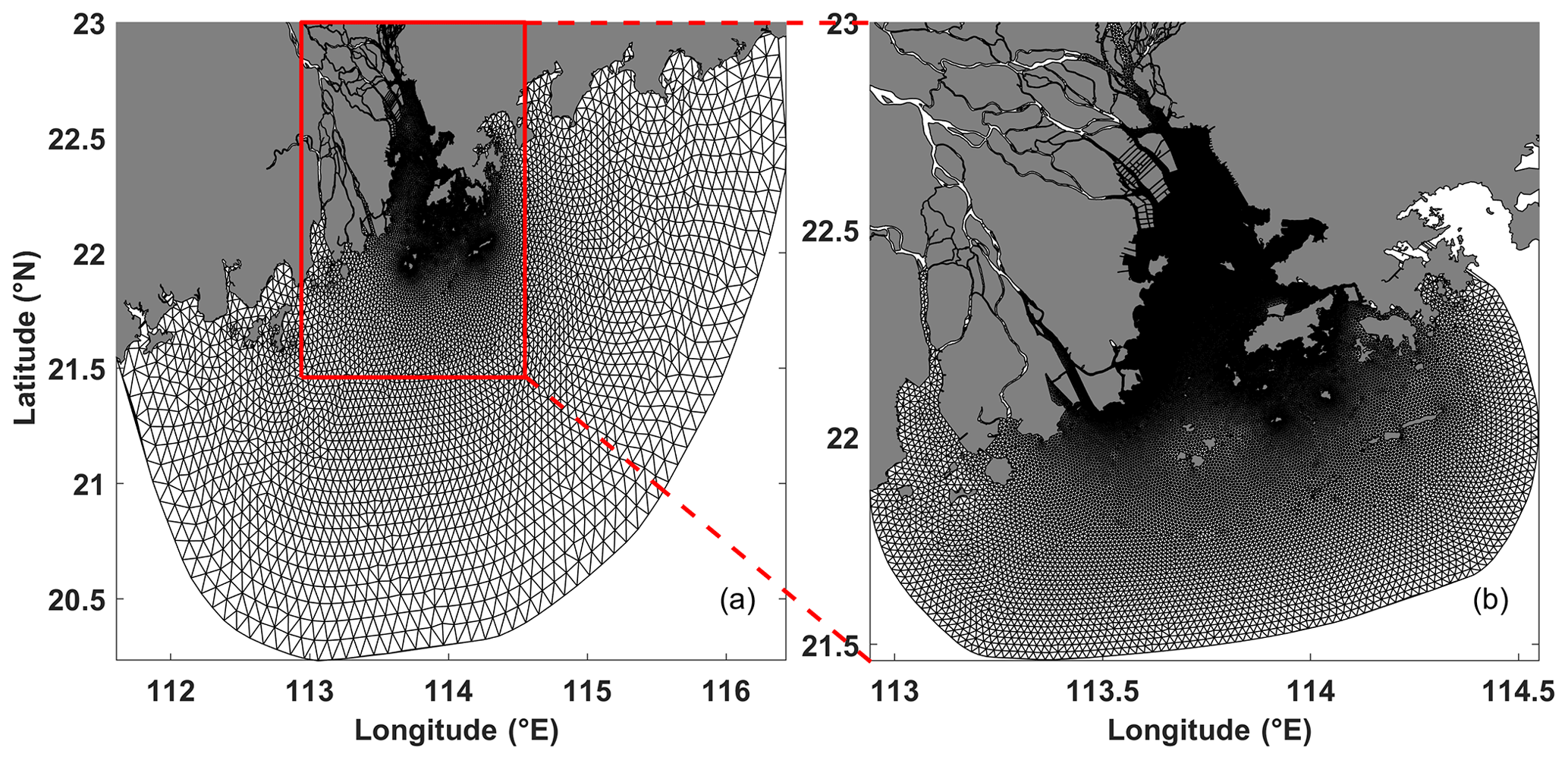
Figure 1 (a) Coarse mesh model. (b) Fine mesh model.

The model incorporates eight major tidal constituents, namely M₂, N₂, S₂, K₂, K₁, O₁, P₁, and Q₁, as tidal driving forces at the open boundary. These constituents are obtained from the Oregon State University Tidal Prediction Software (OTPS/TPXO; https://www.tpxo.net/otps, last access: 22 March 2024; Egbert and Erofeeva, 2002). To initialize the model, salinity climatological data from the 1° World Ocean Atlas 2009 (WOA2009) dataset are utilized (https://accession.nodc.noaa.gov/0094866, Levitus, 2013). The wind data used in this study are obtained from the monthly averaged Cross-Calibrated Multi-Platform (CCMP) dataset, which has spatial resolutions of 0.25°×0.25° (http://www.remss.com/measurements/ccmp, last access: 22 March 2024; Mears et al., 2022). The Pearl River Estuary (PRE) experiences seasonal reversing monsoonal winds, as documented by Pan et al. (2014) and Pan and Gu (2016). The monthly averaged CCMP wind data indicate prevalent southwesterly winds during the summer season. Our investigation specifically focuses on the impact of southwesterly winds on the dynamics of Lagrangian residual velocity (LRV). The lateral boundary incorporates monthly averaged river runoff data from eight river inlets, which are provided by the Water Conservancy Commission of the Pearl River under the Ministry of Water Resources. The topography data of the PRE are from the ETOPO2 dataset of NOAA (https://www.ngdc.noaa.gov/mgg/global/relief/ETOPO2/ETOPO2v2-2006/, last access: 22 March 2024; NOAA National Geophysical Data Center, 2006), while the topography within the estuary is derived from electronic nautical chart data provided by the China Maritime Safety Administration.

The coarse-grid model simulates a period from 1 January to 31 August 2017, and it reaches a quasi-steady state after 1 month. In this study, the outputs from the coarse-grid model are utilized as the initial and boundary conditions for the fine-grid model. The fine-grid model, which begins on 1 June 2017, stabilizes after 1 month. The analysis focuses on the results from the fine-grid model obtained on 24 July 2017 during spring tides and 2 August 2017 during neap tides. A split-mode time-stepping method is employed with 2 s external and 10 s internal time steps for the coarse-grid model. The fine-grid model uses a 0.5 s external time step, which is half of the time step used in the coarse-grid model. The bottom friction in the model is based on the quadratic bottom friction law, and the calculation of the eddy viscosity coefficient employs the Mellor–Yamada level 2.5 turbulence closure model.

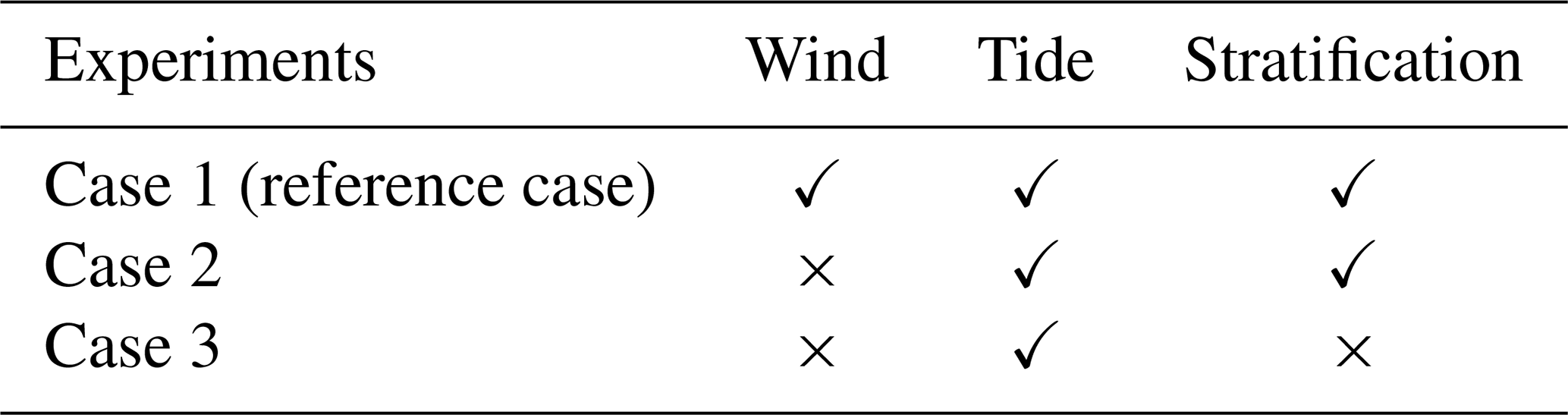
To investigate the effects of wind and stratification on the dynamics of LRV, Case 1 (reference case) includes wind forcing and periodic stratification. Case 2 examines the influence of wind by removing wind forcing compared to Case 1. Case 3 explores the effects of stratification by imposing a uniformly constant salinity and temperature without considering river discharge compared to Case 2 (Table 1). The constant salinity and temperature, with values of 32 psu and 28 °C, respectively, are derived by averaging WOA2009 data for July and August across the whole domain.

Table 1 Numerical experiment scenarios.

2.3 Model verification

The PRE is oriented in the north–south direction (Fig. 2). Accordingly, the positive x axis, u, and u_L are directed eastward; the positive y axis, v, and v_L are directed northward; and the positive z axis, w, and w_L are directed upward. In this context, u and v correspond to the cross-estuary and along-estuary velocities, respectively, with u_L and v_L denoting the corresponding LRV. The paper selects four sections, including three cross sections (Sections B–D) and one along-estuary section (Section A), which roughly cover the PRE (black lines in Fig. 2a). The examination of LRV components and the eddy viscosity subcomponent is presented solely in Section C, given the uniform conclusions derived across four sections. Moreover, the chosen cross section, Section C, aptly depicts the differential dynamics of LRV between the shoal and the deep channel.

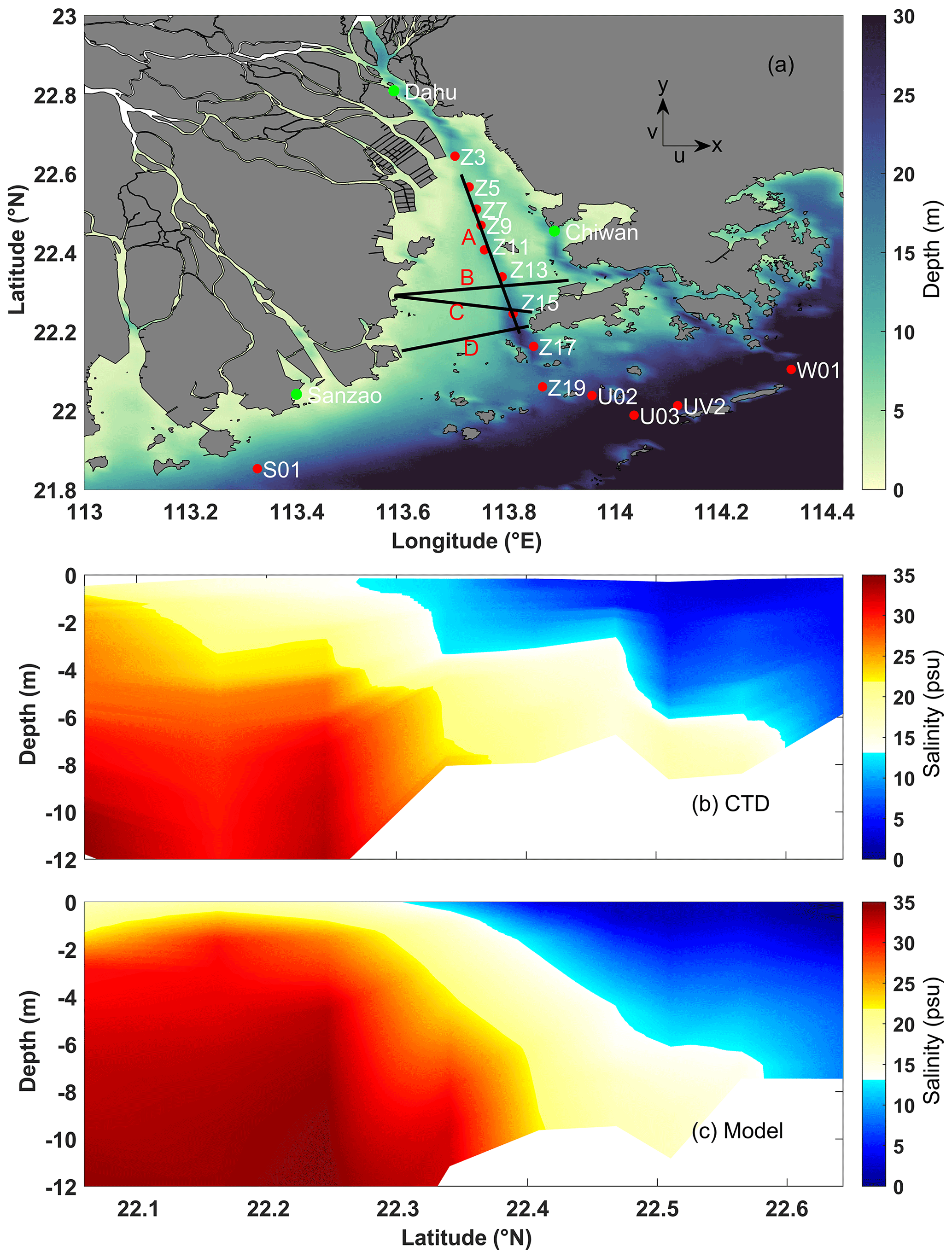
Figure 2 (a) Bathymetry of the model domain. Black lines mark sections for result analysis. Green dots indicate tide gauge stations for elevation validation, and red dots indicate CTD positions for salinity verification. (b) Along-estuary salinity profiles based on CTD-profiled data, closely aligned with Section A; (c) salinity outputs from the numerical model.

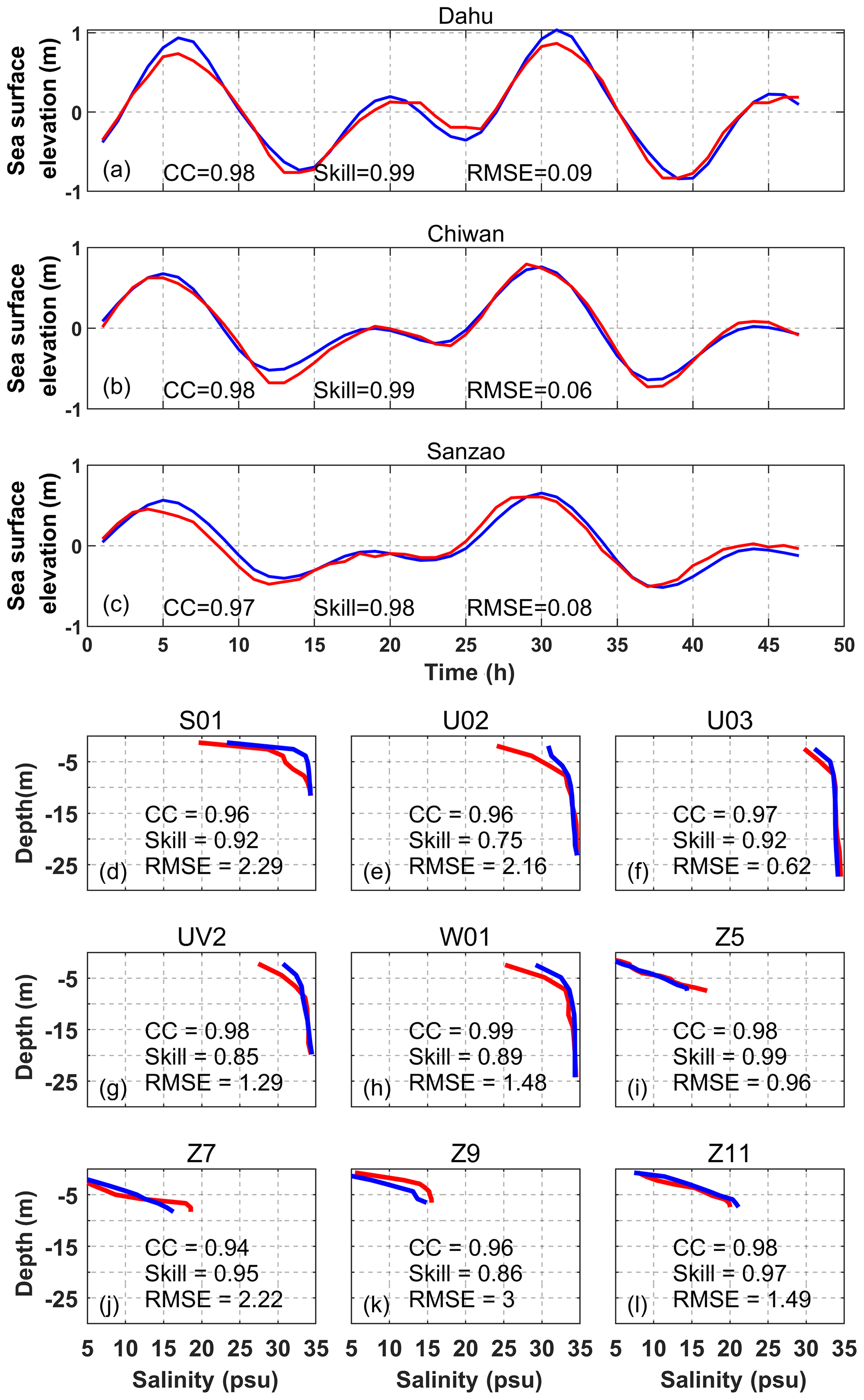
Figure 3 Comparisons between the observed (red line) and modeled (blue line) elevation and salinity. The three parameters including correlation coefficient (CC), Willmott skill score (Skill), and RMSE are calculated at each station.

Model verification involves comparing the model-derived sea surface elevation and salinity with the corresponding observed values from the tide gauge and CTD (conductivity, temperature, and depth) stations, respectively (Fig. 3). The observed sea surface elevation data are collected between 2 and 4 August 2017, and the observed salinity data are acquired through CTD profiling from 4 to 6 August 2017. A good agreement between the model and observed values highlights the effectiveness of the model (Fig. 3). To further assess the model's performance, three statistical parameters are calculated: the correlation coefficient (CC), Willmott skill score (Willmott, 1981), and root mean square error (RMSE). These parameters quantify the model's accuracy and skill:

$$\begin{array}{}\text{(4)}& {\displaystyle }\mathrm{CC}={\displaystyle \frac{{\sum }_{i=\mathrm{1}}^N\left({\mathrm{ob}}_i-\stackrel{\mathrm{‾}}{\mathrm{ob}}\right)\left({\mathrm{mo}}_i-\stackrel{\mathrm{‾}}{\mathrm{mo}}\right)}{\sqrt{{\sum }_{i=\mathrm{1}}^N{\left({\mathrm{ob}}_i-\stackrel{\mathrm{‾}}{\mathrm{ob}}\right)}^{\mathrm{2}}{\sum }_{i=\mathrm{1}}^N{\left({\mathrm{mo}}_i-\stackrel{\mathrm{‾}}{\mathrm{mo}}\right)}^{\mathrm{2}}}}},\text{(5)}& {\displaystyle }\mathrm{Skill}=\mathrm{1}-{\displaystyle \frac{{\sum }_{i=\mathrm{1}}^N{\left({\mathrm{ob}}_i-{\mathrm{mo}}_i\right)}^{\mathrm{2}}}{{\sum }_{i=\mathrm{1}}^N{\left(\left|{\mathrm{mo}}_i-\stackrel{\mathrm{‾}}{\mathrm{ob}}\right|+\left|{\mathrm{ob}}_i-\stackrel{\mathrm{‾}}{\mathrm{ob}}\right|\right)}^{\mathrm{2}}}},\end{array}$$

and

$$\begin{array}{}\text{(6)}& \mathrm{RMSE}=\sqrt{{\displaystyle \frac{\mathrm{1}}{N}}\sum _{i=\mathrm{1}}^N{\left({\mathrm{ob}}_i-{\mathrm{mo}}_i\right)}^{\mathrm{2}}},\end{array}$$

where ob_i and mo_i are the observed data and model data, respectively; $\stackrel{\mathrm{‾}}{\mathrm{ob}}$ and $\stackrel{\mathrm{‾}}{\mathrm{mo}}$ are the average value of the observed data and the model data; and N represents the number of observations. The performance assessments of the modeled tidal elevation are presented in Fig. 3a–c. The model demonstrates a reasonable match with the observed tidal elevations, exhibiting good performance with a skill score greater than 0.98, a correlation coefficient exceeding 0.97, and a root mean square error less than 0.09 m. This indicates that the model performs well in simulating tidal elevations. The assessments of the model's performance in simulating salinity are depicted in Figs. 2b and c and 3d–l. The correlation coefficients for salinity are higher than 0.94, with the majority of skill scores exceeding 0.85 and root mean square errors less than 3 psu. The model exhibits good performance in simulating salinity.

3 Results

3.1 Contributions of dominant components for LRV

To quantify the contribution of each dynamic component of the LRV, the absolute values of each component are averaged throughout Section C in this study, as follows:

$$\begin{array}{}\text{(7)}& M\left(\cdot \right)={\displaystyle \frac{\mathrm{1}}{B}}\int \mathrm{abs}\left(\cdot \right)\mathrm{d}B,\end{array}$$

where abs is the absolute value function, the symbol ⋅ can be replaced by each dynamic component of the LRV, and B represents the area of the cross section.

Figure 4 illustrates the decomposition of cross-estuary LRV into dominant contributions for the reference case. During neap tides, the eddy viscosity component (u_Ltu) exhibits a two-layer structure with eastward flow in the upper layer and westward flow in the lower layer (Fig. 4a). The barotropic pressure gradient component (u_Lba) generally flows westward in most areas of the shoal, while it displays an eastward flow in the upper layer and a westward flow in the lower layer of the deep channel (Fig. 4b). The two-layer structure of u_Lba arises from the distinct trajectories of particles in the upper and lower layers. The integration results along these different trajectories produce varying magnitudes and opposite directions of u_Lba components in both layers. Conversely, the contribution from the baroclinic pressure gradient (u_Lgr; Fig. 4c) opposes u_Lba. During spring tides, the structure of the three components, namely u_Ltu, u_Lba, and u_Lgr, remains analogous to that during neap tides throughout the cross section (Fig. 4j–l). During both spring and neap tides, the three striking components (u_Ltu, u_Lgr, and u_Lba) are aggregated (Fig. 4e and n) and compared to the total LRV obtained directly from the model based on the Lagrangian particle tracking algorithms (Fig. 4d and m). It is observed that u_L primarily arises from an imbalance between u_Ltu, u_Lgr, and u_Lba. The eastward exchange circulation is predominantly attributed to u_Ltu in the upper layer of the shoal, while the westward flow in the lower layer of the shoal is primarily driven by u_Ltu and u_Lba. In the upper layer of the deep channel, the eastward flow is determined by the interplay of u_Lba and u_Ltu, which also induces the westward flow in the lower layer of the channel. Notably, u_Lgr predominantly counteracts u_Lba.

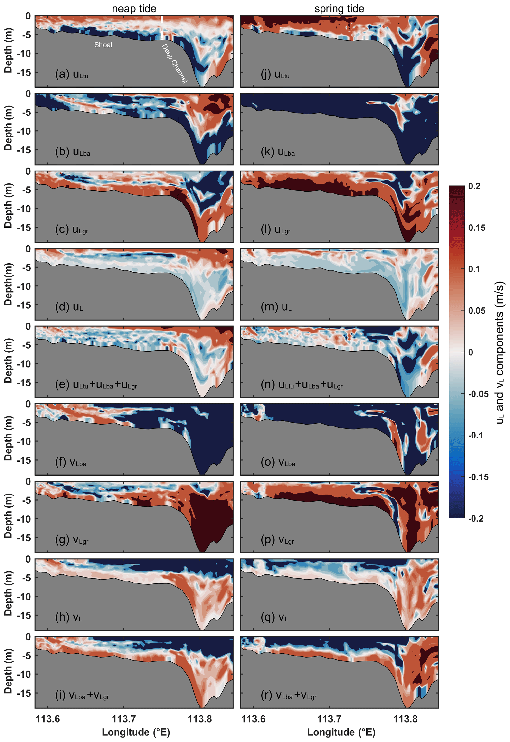
Figure 4 Dominant components of u_L and v_L in Section C for Case 1. For cross-estuary components, (a, j) eddy viscosity component (u_Ltu); (b, k) barotropic component (u_Lba); (c, l) baroclinic component (u_Lgr); (d, m)  total LRV (u_L) directly obtained by the model; and (e, n) cumulative sum of u_Ltu, u_Lba, and u_Lgr. For along-estuary components, (f, o) barotropic pressure gradient component (v_Lba), (g, p) baroclinic pressure gradient component (v_Lgr), (h, q) total LRV (v_L) obtained directly by the model, and (i, r) cumulative sum of v_Lba and v_Lgr. The components in (a–i) represent neap tides, while those in (j–r) represent spring tides. For cross-estuary components, red shading indicates eastward flow, and blue shading indicates westward flow. For along-estuary components, red shading signifies inflow, while blue shading denotes outflow.

The decomposition of along-estuary LRV into dominant contributions is depicted in Fig. 4 for the reference case. During neap tides, the barotropic pressure gradient component (v_Lba) contributes to an up-estuary flow in most areas of the shoal and a down-estuary flow in the deep channel (Fig. 4f); the baroclinic pressure gradient component (v_Lgr) exhibits a two-layer circulation with the seaward flow in the upper layer and landward flow in the lower layer of the shoal along with inflow in most areas of the deep channel (Fig. 4g). It shows the opposite pattern to v_Lba. During spring tides, there is a down-estuary flow of v_Lba in the shoal, which is contrary to the flow pattern during neap tides (Fig. 4o). Additionally, the outflow area of v_Lgr in the upper layer of the shoal is smaller during spring tides than during neap tides (Fig. 4p). During both spring and neap tides, the sum of v_Lba and v_Lgr (Fig. 4i and r) closely resembles the total along-estuary LRV (v_L; Fig. 4h and q). Therefore, the dominant components of v_L are v_Lba and v_Lgr. Since these components must balance across the estuary, the outflow in the upper layer is mainly determined by v_Lba, while the inflow in the lower layer is induced by v_Lgr.

The intensities of the exchange flows are quantified in Fig. 5 for the reference case. During spring tides, the magnitude of u_Ltu is approximately 2 times higher than that during neap tides, the magnitude of u_Lgr nearly doubles compared to that during neap tides, and the magnitude of u_Lba is roughly 4 times as large as that during neap tides. Among the dominant components of u_L, u_Lba exhibits the most pronounced contributions, being 1–2 times as strong as u_Ltu and u_Lgr. During spring tides, the magnitudes of v_Lba and v_Lgr are about 1.4 times as large as those during neap tides. The contributions from gravitational circulation and barotropic pressure gradient component to total LRV are of the same magnitude.

Figure 5 Bar charts for the magnitude of each component of u_L and v_L.

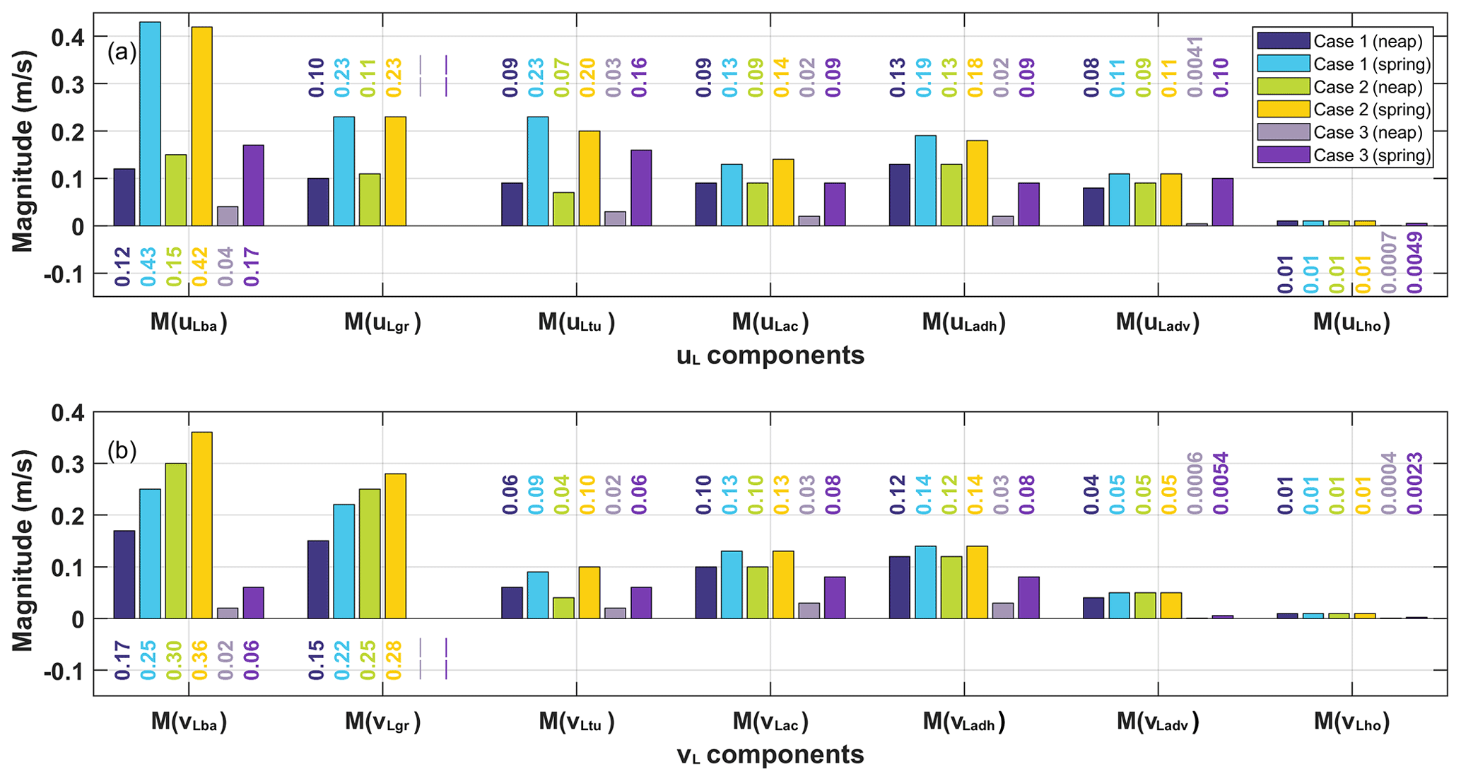
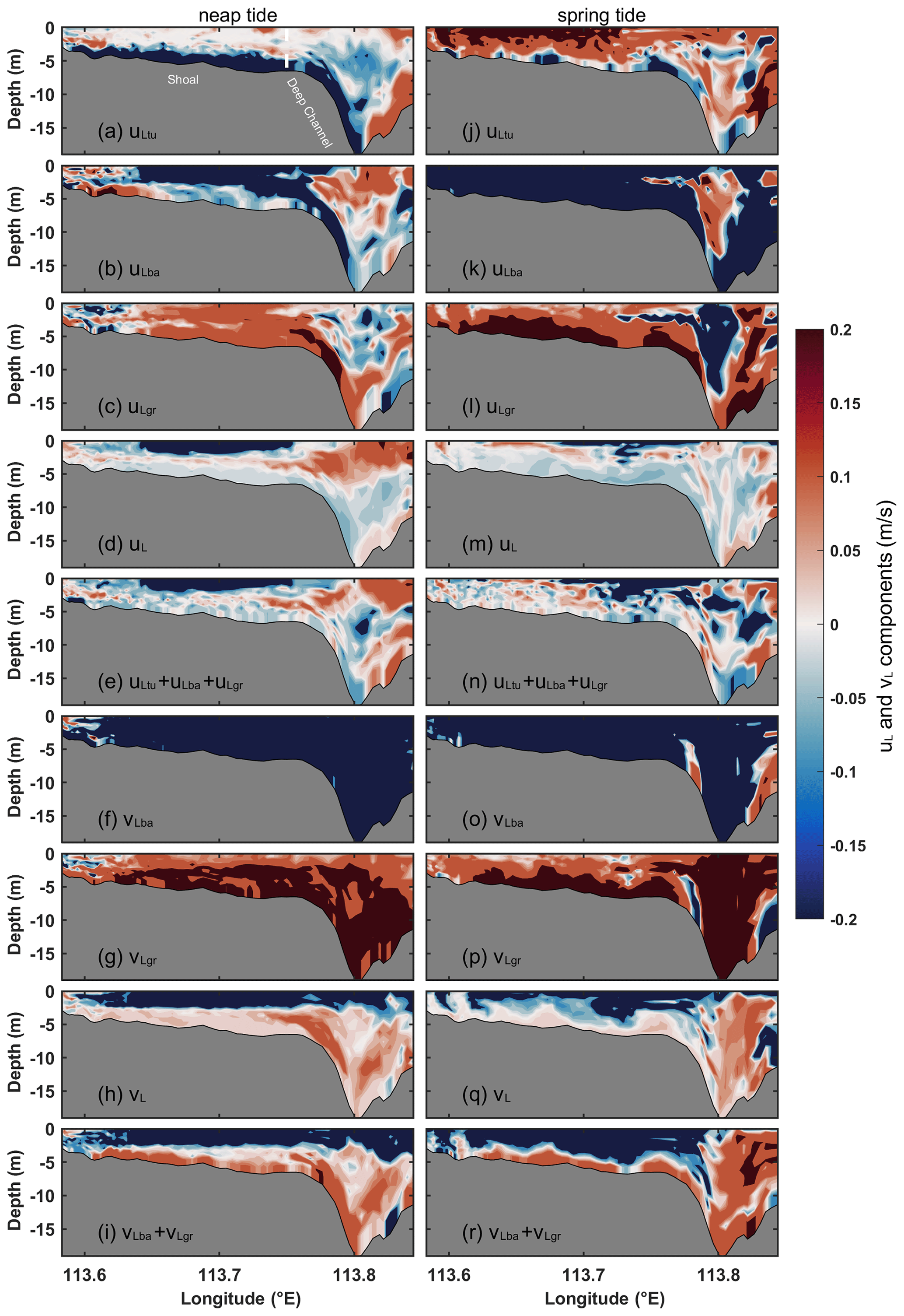
Figure 6 Same as Fig. 4, but for Case 2 without wind forcing.

Neglecting the influence of wind, the cross-estuary and along-estuary dominant components are displayed in Fig. 6 for Case 2. The eddy viscosity component (u_Ltu) exhibits a similar pattern to the reference case during both neap and spring tides (Fig. 6a and j). However, during neap tides, the magnitude of the eastward flow of u_Ltu in the upper 2 m is approximately 1 order of magnitude smaller than that in Case 1 (Fig. 6a vs. Fig. 4a), although the absolute value of u_Ltu averaged in Section C for Case 2 is slightly different compared to that in Case 1 (Fig. 5). This suggests that wind primarily affects the upper exchange circulation by influencing the mixing of the upper water column. During spring tides, u_Ltu shows small differences in magnitude between Case 1 and Case 2 (Fig. 6j vs. Fig. 4j), indicating that wind has a slight influence on exchange flow during spring tides. During both spring and neap tides, the structures and magnitudes of the barotropic pressure gradient component (u_Lba; Fig. 6b and k) and the baroclinic pressure gradient component (u_Lgr; Fig. 6c and l) are similar to those in Case 1. When wind effects are not considered, the structure of the cross-estuary LRV (u_L) (Fig. 6d and m) is still determined by the combined contributions of u_Lba, u_Lgr, and u_Ltu (Fig. 6e and n). However, the eastward flow determined by u_Ltu in the upper layer of the shoal in Case 1 transforms into a westward flow primarily driven by u_Lba in Case 2.

The v_Lba changes from inflow in Case 1 to outflow in the shoal during neap tides (Fig. 6f). Similarly, v_Lgr shifts from outflow in Case 1 to inflow in the upper layer of the shoal during neap tides in Case 2 (Fig. 6g). This suggests that wind plays a crucial role in the components of LRV in the upper water column of the shoal. During spring tides, v_Lba and v_Lgr maintain the same structure as observed in Case 1 (Fig. 6o and p), indicating that wind is unimportant during spring tides. The structure of the along-estuary LRV (v_L) (Fig. 6h and q) is primarily determined by the combined contributions of v_Lba and v_Lgr (Fig. 6i and r), analogous to that in Case 1. But in the absence of wind, the magnitudes of v_Lba and v_Lgr are larger than those in Case 1, indicating that southwesterly wind suppresses gravitational circulation. The relative contributions of v_Lba and v_Lgr to v_L are approximately equal (Fig. 5).

The stratification and wind forcing are ignored in Case 3. The dominant components of the cross-estuary LRV in Section C are shown in Fig. 7. During neap tides, the local acceleration component (u_Lac) predominantly exhibits eastward flow in most areas, with minor regions showing westward flow in the shoal and deep channel (Fig. 7a). Conversely, during spring tides, a prevailing westward flow characterizes the majority of the shoal regions, while an eastward flow prevails in the deep channel (Fig. 7g). These results highlight the profound impact of tides on the structure of u_Lac in a homogeneous water column. Comparing the results with those of Case 2, u_Lac undergoes a transition from vertically sheared flow in Case 2 to horizontally sheared flow in Case 3, indicating that stratification plays a notable role in shaping the structure of u_Lac. The horizontal nonlinear advective component (u_Ladh) exhibits a flow pattern that is the reverse of u_Lac (Fig. 7b and h). The barotropic pressure gradient component (u_Lba) primarily shows unidirectional westward flow throughout the cross section (Fig. 7c and i). The pattern of u_Lba in the shoal and most of the lower layer of the deep channel is consistent with that observed in Case 2. However, in the upper layer of the deep channel, u_Lba transforms eastward flow in Case 2 into westward flow in Case 3. The eddy viscosity component (u_Ltu) induces a flow opposite to that of u_Lba (Fig. 7d and j), which differs from the vertically sheared flow observed in Case 2.

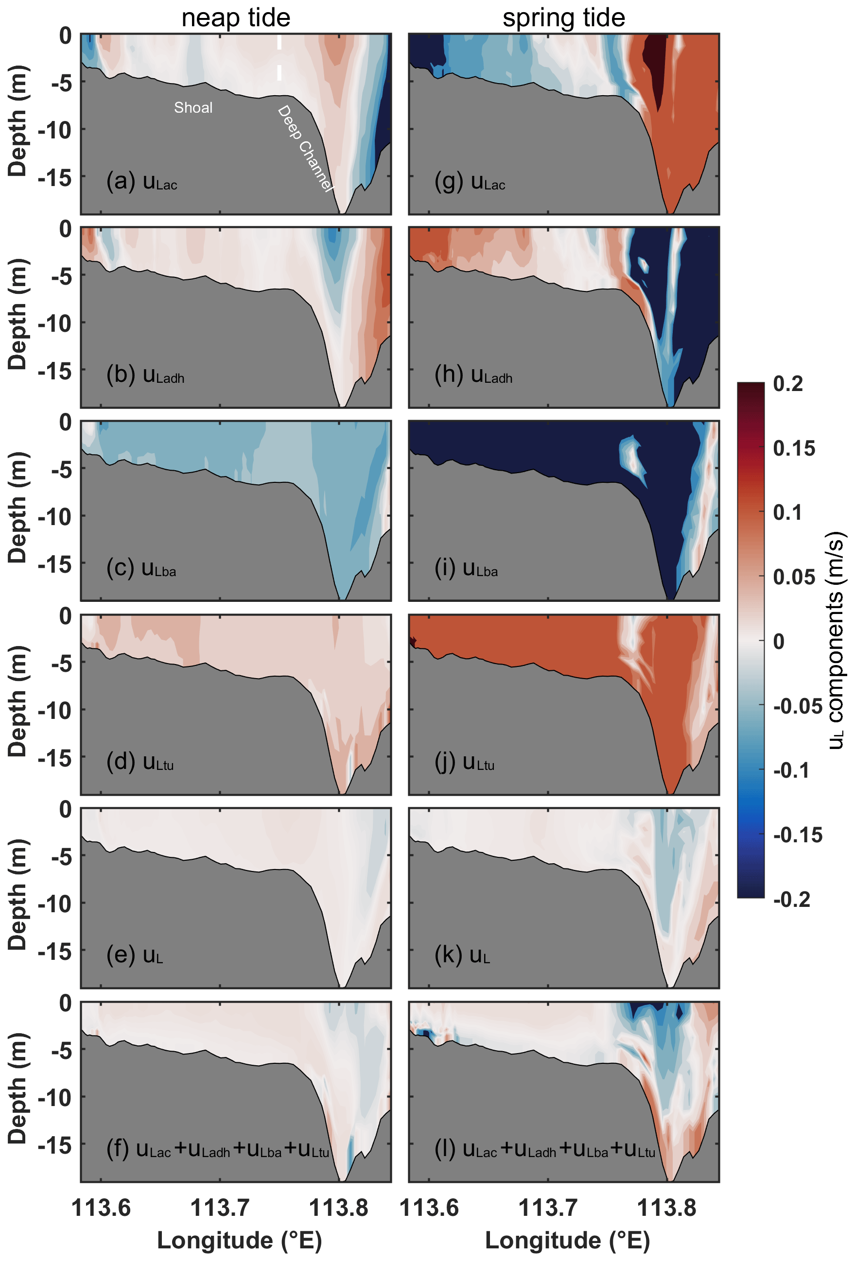
Figure 7 Dominant components of u_L in Section C for Case 3. (a, g) Local acceleration component (u_Lac); (b, h) horizontal nonlinear advection component (u_Ladh); (c, i) barotropic pressure gradient component (u_Lba); (d, j) eddy viscosity component (u_Ltu); (e, k) the total LRV (u_L) obtained directly by the model; and (f, l) the sum of u_Lac, u_Ladh, u_Lba, and u_Ltu during (a–f) neap and (g–l) spring tides. Red shading represents eastward flow, and blue shading represents westward flow.

The structure of the cross-estuary LRV (u_L) (Fig. 7e and k) closely resembles the structure of the sum of the four components: u_Lac, u_Ladh, u_Lba, and u_Ltu in Case 3 (Fig. 7f and l). This indicates that the overall structure of u_L (Fig. 7e and k) is primarily determined by the combined effects of these four components. Among them, the eastward flow in the shoal and the lower layer of the deep channel is mainly determined by u_Ltu (Fig. 7d and j), with u_Lac playing a secondary role (Fig. 7a and g). On the other hand, the westward flow in the upper layer of the deep channel is primarily influenced by u_Lba (Fig. 7c and i), with u_Ladh contributing as a secondary component (Fig. 7b and h).

The magnitudes of u_Lac, u_Ladh, and u_Lba during spring tides are approximately 4 times as large as those during neap tides in Case 3 (Fig. 5). The magnitude of u_Ltu during spring tides is approximately 5-fold compared to neap tides. The relative contributions of u_Lba and u_Ltu to u_L are roughly equal, and u_Lac and u_Ladh have similar contributions. Moreover, the contribution of u_Lba is approximately 1–2 times as large as that of u_Lac in Case 3.

During both spring and neap tides, the along-estuary barotropic pressure gradient component (v_Lba) exhibits outflow in most areas in Case 3 (Fig. 8a and e), which is similar to Case 2, indicating that stratification has minimal effects on the structure of v_Lba. The eddy viscosity component (v_Ltu) shows a nearly opposite pattern compared to v_Lba (Fig. 8b and f). Compared to Case 2, v_Ltu exhibits an opposite pattern at the bottom of the shoal and in the deep channel. The imbalance between the two components, v_Lba and v_Ltu (Fig. 8d and h), determines the along-estuary circulation (v_L) (Fig. 8c and g). The inflow in the shoal is primarily driven by v_Ltu, while the outflow in the deep channel is dominated by v_Lba. During spring tides, the magnitudes of v_Lba and v_Ltu are about 3-fold that during neap tides in Case 3 (Fig. 5). During neap and spring tides, the relative contributions of v_Lba and v_Ltu to v_L are equal.

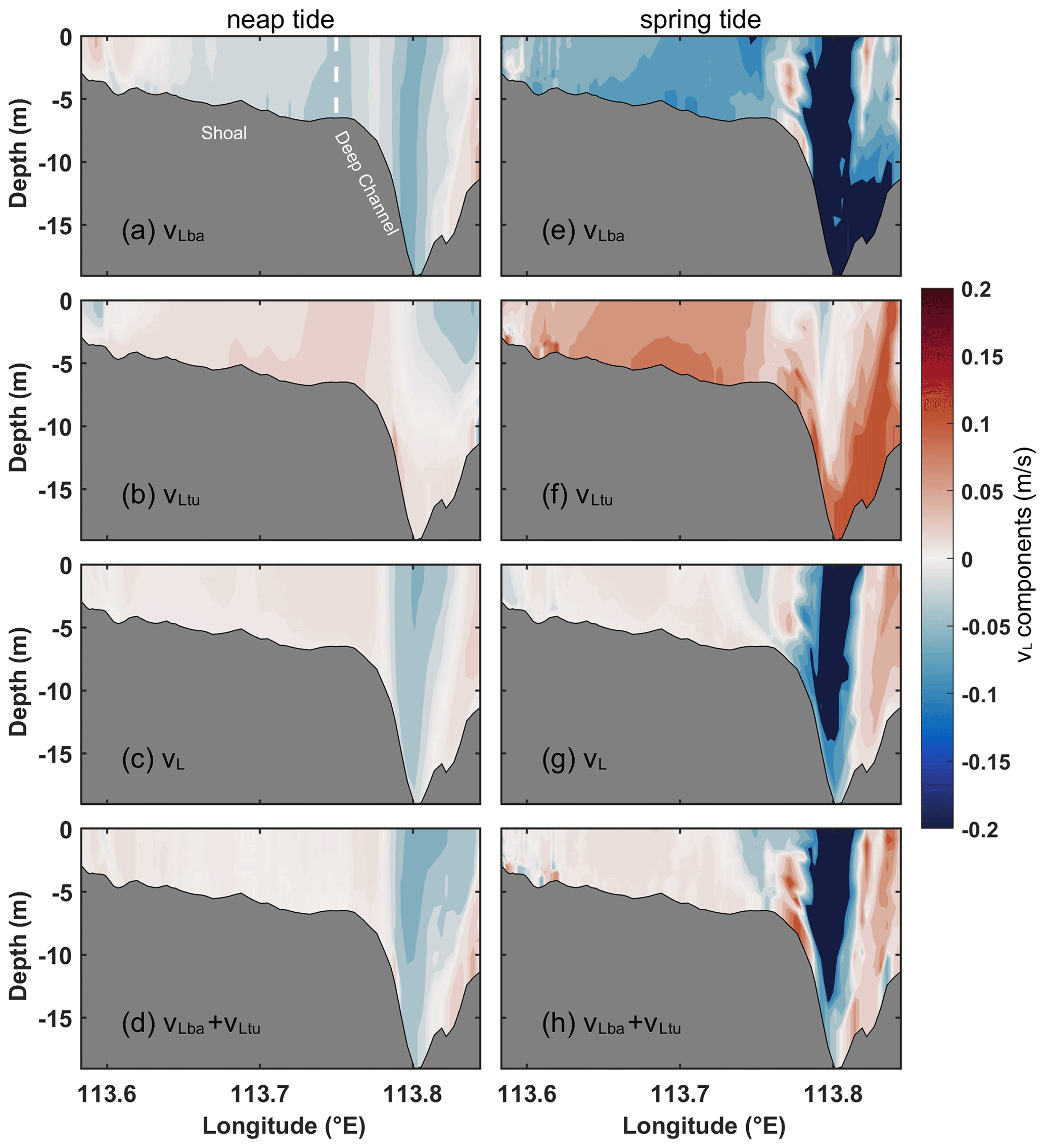
Figure 8 Dominant components of v_L in Section C for Case 3. (a, e) Barotropic pressure gradient component (v_Lba), (b, f) eddy viscosity component (v_Ltu), (c, g) total LRV obtained directly by the model, and (d, h) the sum of v_Lba and v_Ltu during (a–d) neap and (e–h) spring tides. Red shading represents inflow, and blue shading represents outflow.

3.2 Contributions of non-dominant components for LRV

The analysis of the contributions from non-dominant components to LRV for Case 1 is depicted in Fig. 9. During neap tides, the local acceleration (u_Lac) induces eastward flow in the majority of the upper layer and westward flow in the lower layer (Fig. 9a). Conversely, the horizontal nonlinear advection component (u_Ladh) exhibits an opposite pattern to u_Lac across most regions (Fig. 9b). Meanwhile, the vertical nonlinear advective component (u_Ladv) serves as a sandwiched structure, characterized by vertically staggered eastward and westward flow (Fig. 9c). The combined configuration of u_Lac and u_Ladh contrasts with that of u_Ladv, yielding a relatively small and negative contribution from the sum of these three components (Fig. 9d) to u_L (Fig. 4d). Consequently, the three components are denoted as non-dominant components. The magnitudes of the non-dominant components of u_L during spring tides are slightly larger than those during neap tides. The general patterns of these three components during spring tides resemble those during neap tides except for some areas (Fig. 9h–j). Moreover, during both spring and neap tides, the horizontal diffusion component (u_Lho) is smaller compared to the other components (not shown), and its contribution is negligible. For along-estuary non-dominant components, the combination of the local acceleration component (v_Lac), the horizontal nonlinear advective component (v_Ladh), and the vertical nonlinear term (v_Ladv) (Fig. 9f) contributes less to total LRV (Fig. 4h) and negatively during neap tides. Additionally, the eddy-viscosity-induced flow (v_Ltu) during neap tides exhibits a vertical shear structure, with outflow in the upper and lower layer and inflow in the middle layer (Fig. 9e). During spring tides, the overall structures for each non-dominant component slightly differ from those during neap tides except for some upper areas, and the magnitudes during spring tides exceed those recorded during neap tides (Fig. 9l and m). For both spring and neap tides, the contributions of the horizontal diffusion components (v_Lho) are negligible (not shown). Moreover, the contribution of v_Ltu is relatively smaller compared to their respective dominant components (Fig. 5). In the absence of wind effects, the structure and contribution of each non-dominant component of the LRV in Case 2 closely resemble those observed in Case 1 during both spring and neap tides (not shown), with the exception of the noticeably reduced along-estuary eddy viscosity component (v_Ltu) by 1 order of magnitude in the upper layer in Case 2 during neap tides (Fig. 9g) and slightly intensified during spring tides (Fig. 9n) compared to scenarios with wind. These indicate that wind has a weak influence on the non-dominant components of cross-estuary circulation except for v_Ltu.

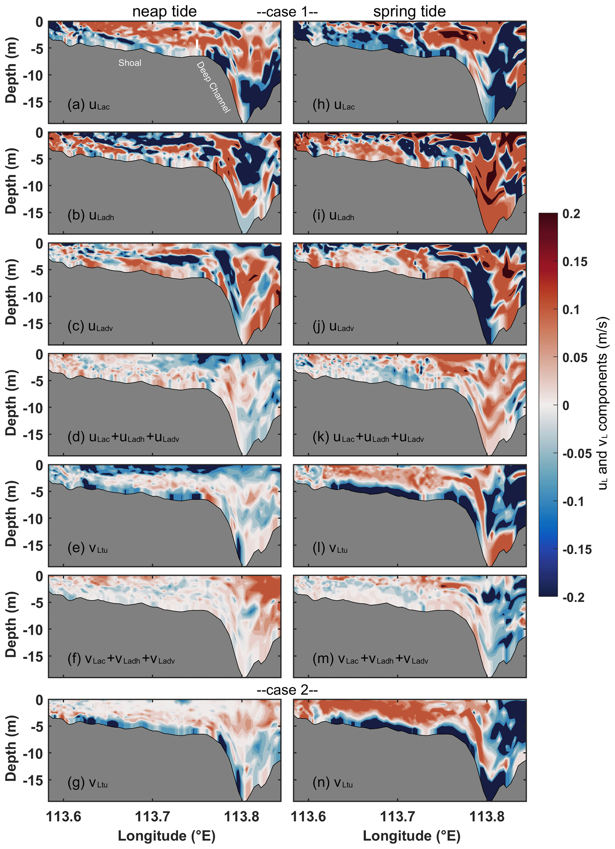
Figure 9 Non-dominant components of u_L and v_L in Section C for Cases 1 and 2. For cross-estuary components in Case 1, (a, h) local acceleration component (u_Lac); (b, i) horizontal nonlinear advection component (u_Ladh); (c, j) vertical nonlinear advection component (u_Ladv); and (d, k) the sum of u_Lac,u_Ladh, and u_Ladv during (a–d) neap and (h–k) spring tides. For along-estuary components in Case 1, (e, l) eddy viscosity component (v_Ltu) and (f, m) the sum of $v_{\mathrm{Lac}},v_{\mathrm{Ladh}},$ and v_Ladv during (e, f) neap and (l, m) spring tides. Along-estuary (g, n) eddy viscosity component (v_Ltu) in Case 2 during (g) neap and (n) spring tides. The shading follows the same format as presented in Fig. 4.

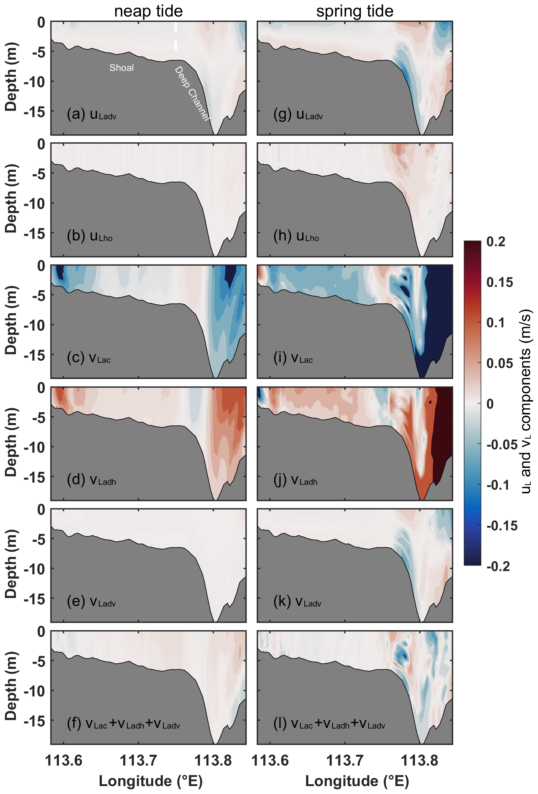
Figure 10 Non-dominant components of u_L and v_L in Section C for Case 3. For cross-estuary components, (a, g) vertical nonlinear advection component (u_Ladv) and (b, h) horizontal diffusion component (u_Lho). For along-estuary components, (c, i) local acceleration component (v_Lac); (d, j) horizontal advection component (v_Ladh); (e, k) vertical advection component (v_Ladv); and (f, l) the sum of v_Lac, v_Ladh, and v_Ladv during (a–f) neap and (g–l) spring tides. The shading follows the same format as presented in Fig. 4.

Neglecting wind forcing and stratification, the magnitudes of the vertical nonlinear advection component (u_Ladv) and horizontal diffusion component (u_Lho) are relatively low during both spring and neap tides. Compared to Case 2, the magnitude of u_Lho (Fig. 10b and h) in Case 3 is reduced by approximately half during spring tides and by a factor of 14 during neap tides, while the magnitude of u_Ladv (Fig. 10a) in Case 3 experiences an approximately 20-fold reduction during neap tides (Fig. 5). For both neap and spring tides, v_Lac shifts from inflow in Case 2 to outflow in Case 3 in some areas of the shoal (Fig. 10c and i). The horizontal nonlinear advection component (v_Ladh) in Case 3 exhibits a pattern opposite to that of v_Lac (Fig. 10d and j). Their combined contributions of these two components to total LRV can be disregarded (Fig. 10f and l). The contributions from the vertical nonlinear advection component (v_Ladv; Fig. 10e and k) and horizontal diffusion component (v_Lho; not shown) during spring and neap tides remain relatively low in Case 3. The magnitude of v_Lho in Case 3 is approximately 5-fold smaller during spring tides and 25 times smaller during neap tides than those in Case 2, while the magnitude of v_Ladv in Case 3 experiences an approximately 10-fold reduction during spring tides and an 80-fold reduction during neap tides compared to Case 2 (Fig. 5).

3.3 Contributions of dominant components for the eddy viscosity component

Through an analysis of dominant mechanisms influencing LRV under various dynamic factors, the findings indicate that the cross-estuary eddy viscosity component modulates the configuration of the cross-estuary LRV. In the upper layers, this component exhibits an enhancement of an order of magnitude under the influence of the dominant southwesterly winds, relative to conditions in the absence of wind in the PRE. However, the along-estuary eddy viscosity component is not the predominant contributor to along-estuary LRV under stratified circumstances. In the case of destratification, both the along-estuary and cross-estuary eddy viscosity components play roles in shaping the total LRV. A comprehensive exploration of the dominant mechanisms of the eddy viscosity component entails further decompositions of both the along-estuary and cross-estuary eddy viscosity components into four subgroups. This analysis provides general conclusions and implications for future studies. These subgroups encompass the coupled component of tidal-averaged eddy viscosity and velocity gradient oscillation, the tidal straining component, the turbulent mean component, and the coupled component of tidal-averaged velocity gradient and eddy viscosity oscillation.

During neap tides, the cross-estuary turbulent mean component (u_Lk0u1) for Case 1 displays eastward flows in the upper layer and westward flows in the lower layer (Fig. 11g). During spring tides, u_Lk0u1 closely resembles the pattern observed during neap tides (Fig. 11h). The structure of u_Lk0u1 during neap and spring tides is identical to that of the eddy viscosity (u_Ltu) (Fig. 11a and b). Therefore, u_Ltu is predominantly influenced by u_Lk0u1. During neap tides, the along-estuary turbulent mean component (v_Lk0u1) for Case 1 exhibits a three-layer structure in the shoal, with outflow occurring in the surface and bottom layers and inflow in the middle layer (Fig. 11i). In the deep channel, there is a two-layer flow pattern with outflow in the upper layer and inflow in the lower layer. This structure aligns with that of the eddy viscosity component (v_Ltu) (Fig. 11c). Hence, during neap tides, v_Ltu is primarily influenced by v_Lk0u1. During spring tides, the structure of v_Ltu for Case 1 (Fig. 11d) is contributed by the combined effect of the four components – v_Lk0u0, v_Lk0u1, v_Lk1u0, and v_Lk1u1 (Fig. 11j) – which differs from the structure observed during neap tides. The inflow occurring in the upper layer of the shoal is primarily determined by v_Lk0u0 and v_Lk1u0 (Fig. 11e and f), and the outflow in the lower layer of the shoal is mainly influenced by v_Lk0u1 (Fig. 11k). The structure in the deep channel is primarily determined by v_Lk0u1.

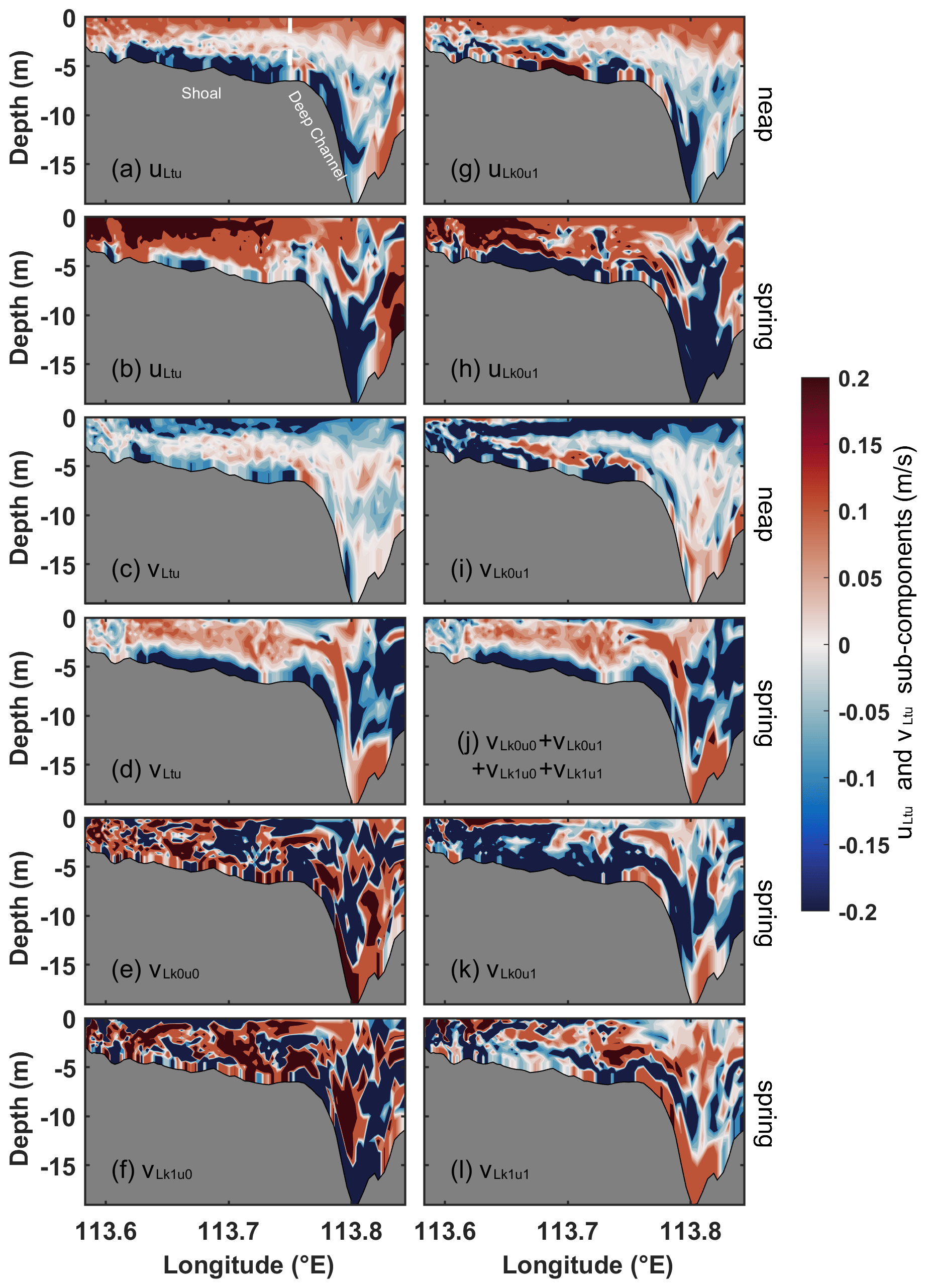
Figure 11 Vertical section of cross-estuary (u_Ltu) and along-estuary (v_Ltu) eddy viscosity components along with their corresponding dominant subcomponents in Section C for Case 1. The u_Ltu during (a) neap and (b) spring tides and (g, h) the corresponding turbulent mean component (u_Lk0u1). (c) v_Ltu and (i) the corresponding turbulent mean component (v_Lk0u1) during neap tides and (d) v_Ltu and (j) the sum of four dominant subcomponents (e, f, k,, l) during spring tides. The shading follows the same format as presented in Fig. 4.

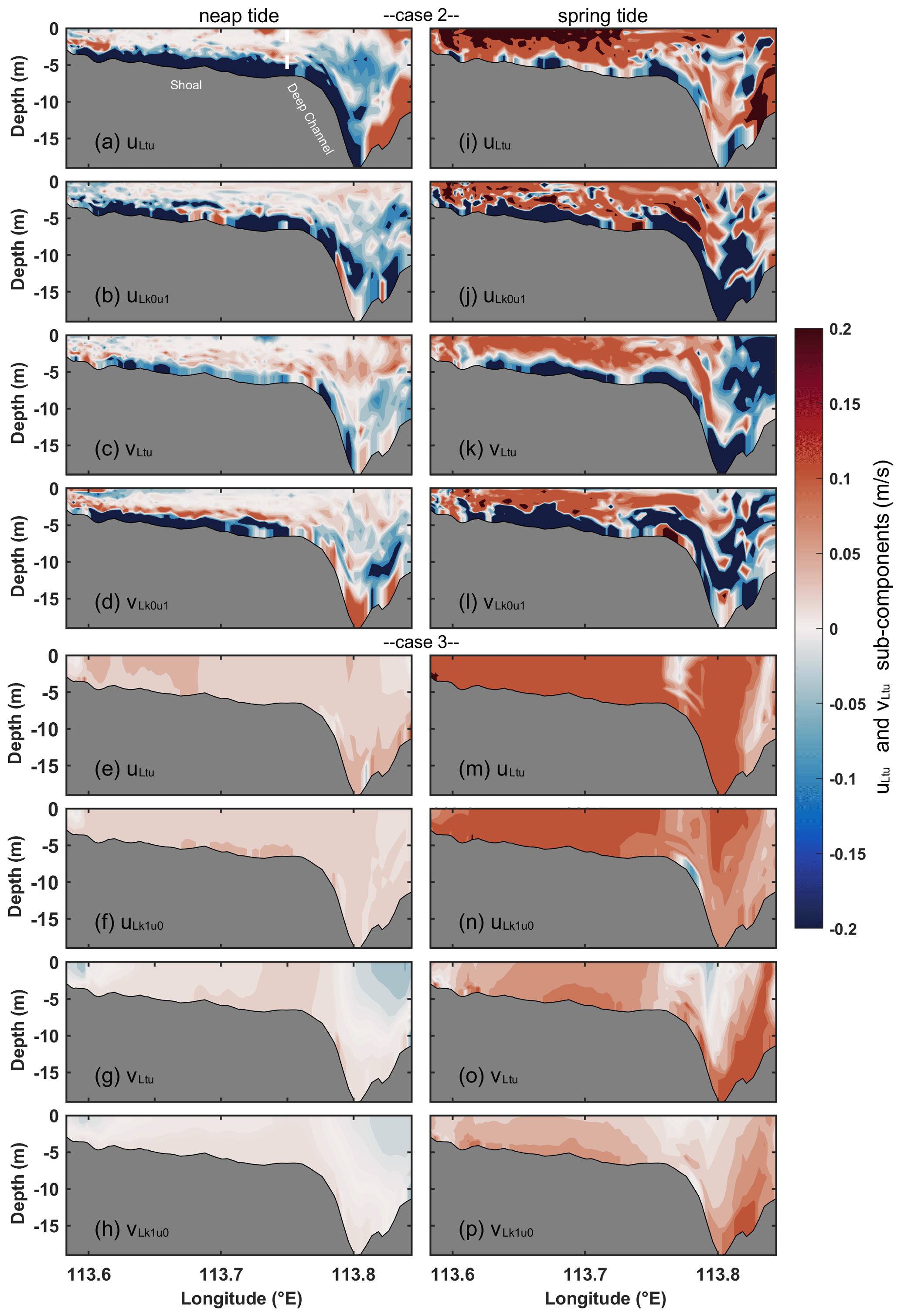
Figure 12 The structure of cross-estuary (u_Ltu) and along-estuary (v_Ltu) eddy viscosity components and the corresponding dominant components in Section C for Cases 2 (a–d, i–l) and 3 (e–h, m–p). For Case 2, the u_Ltu during (a) neap and (i) spring tides and (b, j) the corresponding turbulent mean component (u_Lk0u1); the v_Ltu during (c) neap and (k) spring tides and (d, l) the corresponding turbulent mean component (v_Lk0u1). For Case 3, the u_Ltu during (e) neap and (m) spring tides and (f, n) the corresponding tidal straining component (u_Lk1u0); the v_Ltu during (g) neap and (o) spring tides and (h, p) the corresponding tidal straining component (v_Lk1u0). The shading follows the same format as presented in Fig. 4.

During neap tides, the cross-estuary turbulent mean component (u_Lk0u1) for Case 2 exhibits eastward flow in the upper layer and westward flow in the lower layer (Fig. 12b). This pattern aligns with Case 1. However, the magnitude of the eastward flow in the upper layer of u_Lk0u1 during neap tides is 1 order of magnitude smaller than that observed in Case 1. During spring tides, the structure and magnitude of u_Lk0u1 for Case 2 are similar to those of Case 1 (Fig. 12j), suggesting a weak influence of wind on u_Lk0u1. Similar to Case 1, during both neap and spring tides, the cross-estuary eddy viscosity component (u_Ltu) (Fig. 12a and i) is predominantly determined by u_Lk0u1 (Fig. 12b and j). During neap tides, the along-estuary turbulent mean component (v_Lk0u1) for Case 2 exhibits inflow in the upper layer and outflow in the lower layer (Fig. 12d). The structure of v_Lk0u1 in the lower layer is consistent with that in Case 1, while the structure in the upper layer is opposite to that of Case 1. Without the influence of wind, the structure of v_Lk0u1 in the upper layer shifts from outflow in Case 1 to inflow. During spring tides, the area and magnitude of inflow in the upper layer of v_Lk0u1 for Case 2 are larger than those during neap tides (Fig. 12l). During both neap and spring tides, the along-estuary eddy viscosity component (v_Ltu) (Fig. 12c and k) exhibits the same structure as v_Lk0u1 (Fig. 12d and l). Hence, v_Ltu is predominantly influenced by the turbulent mean component (v_Lk0u1).

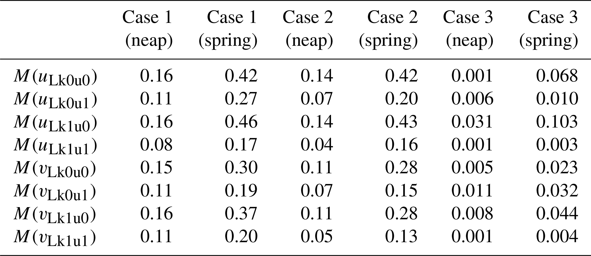
Without consideration of stratification, the cross-estuary tidal straining component (u_Lk1u0) for Case 3 exhibits eastward flow (Fig. 12f) in the shoal during neap tides. The u_Lk1u0 undergoes a transition from westward flow in Case 2 to eastward flow in the lower layer. During spring tides, the u_Lk1u0 for Case 3 maintains the same pattern as observed during neap tides, and its magnitude is greater than that during neap tides (Fig. 12n). During neap tides, the along-estuary tidal straining component (v_Lk1u0) for Case 3 exhibits inflow in most areas of the shoal and shows a two-layer structure in the deep channel with outflow in the upper layer and inflow in the lower layer (Fig. 12h), which is analogous to the structure of v_Lk1u0 in the shoal in Case 2. Stratification mainly affects the structure of v_Lk1u0 in the lower layer of the deep channel. During spring tides, the inflow area of v_Lk1u0 for Case 3 in the deep channel is larger than that during neap tides (Fig. 12p). During both neap and spring tides, the u_Ltu and v_Ltu (Fig. 12e, g, m, and o) align with u_Lk1u0 and v_Lk1u0 (Fig. 12f, h, n, and p), respectively. Hence, u_Ltu and v_Ltu are primarily influenced by u_Lk1u0 and v_Lk1u0, differing from the dominant components in Case 2. Without consideration of stratification, the dominant components of u_Ltu and v_Ltu shift from the turbulent mean components (u_Lk0u1 and v_Lk0u1) in Case 2 to the tidal straining components (u_Lk1u0 and v_Lk1u0) in Case 3. During neap tides, the magnitude of u_Lk1u0 is approximately 5 times smaller than that in Case 2, while the magnitude of v_Lk1u0 is around 14 times smaller than that in Case 2 (Table 2). During spring tides, the magnitude of u_Lk1u0 is roughly 4 times smaller than that in Case 2, and the magnitude of v_Lk1u0 is approximately 6 times smaller than that in Case 2.

Table 2 The magnitude of each subcomponent for the total eddy viscosity component in three scenarios.

3.4 Contributions of non-dominant components for eddy viscosity component

During neap tides, the cross-estuary coupled component of the tidal-averaged eddy viscosity and velocity gradient oscillation (u_Lk0u0) for Case 1 demonstrates a vertically sheared structure in the shoal, with alternating westward and eastward flows (Fig. 13a). During spring tides, u_Lk0u0 for Case 1 predominantly flows eastward in the shoal and displays a two-layer structure in the deep channel with eastward flow in the upper layer and westward flow in the lower layer (Fig. 13c). The cross-estuary tidal straining component (u_Lk1u0) during neap tides exhibits an opposing structure to that of u_Lk0u0 in the lower layer (Fig. 13g). In the upper layer, it displays a similar pattern to u_Lk0u0. During spring tides, the extent and magnitude of the eastward flow of u_Lk1u0 in the deep channel are larger than during neap tides (Fig. 13i). During neap tides, the cross-estuary coupled component of the eddy viscosity oscillation and the tidal-averaged velocity gradient (u_Lk1u1) exhibits a complex vertically sheared structure (Fig. 13b). During spring tides, u_Lk1u1 displays a similar structure but with a greater magnitude than that during neap tides (Fig. 13d). The combined effect of the three components (Fig. 13h and j), namely u_Lk0u0, u_Lk1u0, and u_Lk1u1, contrasts with u_Lk0u1 (Fig. 11g and h) in most areas of the cross section.

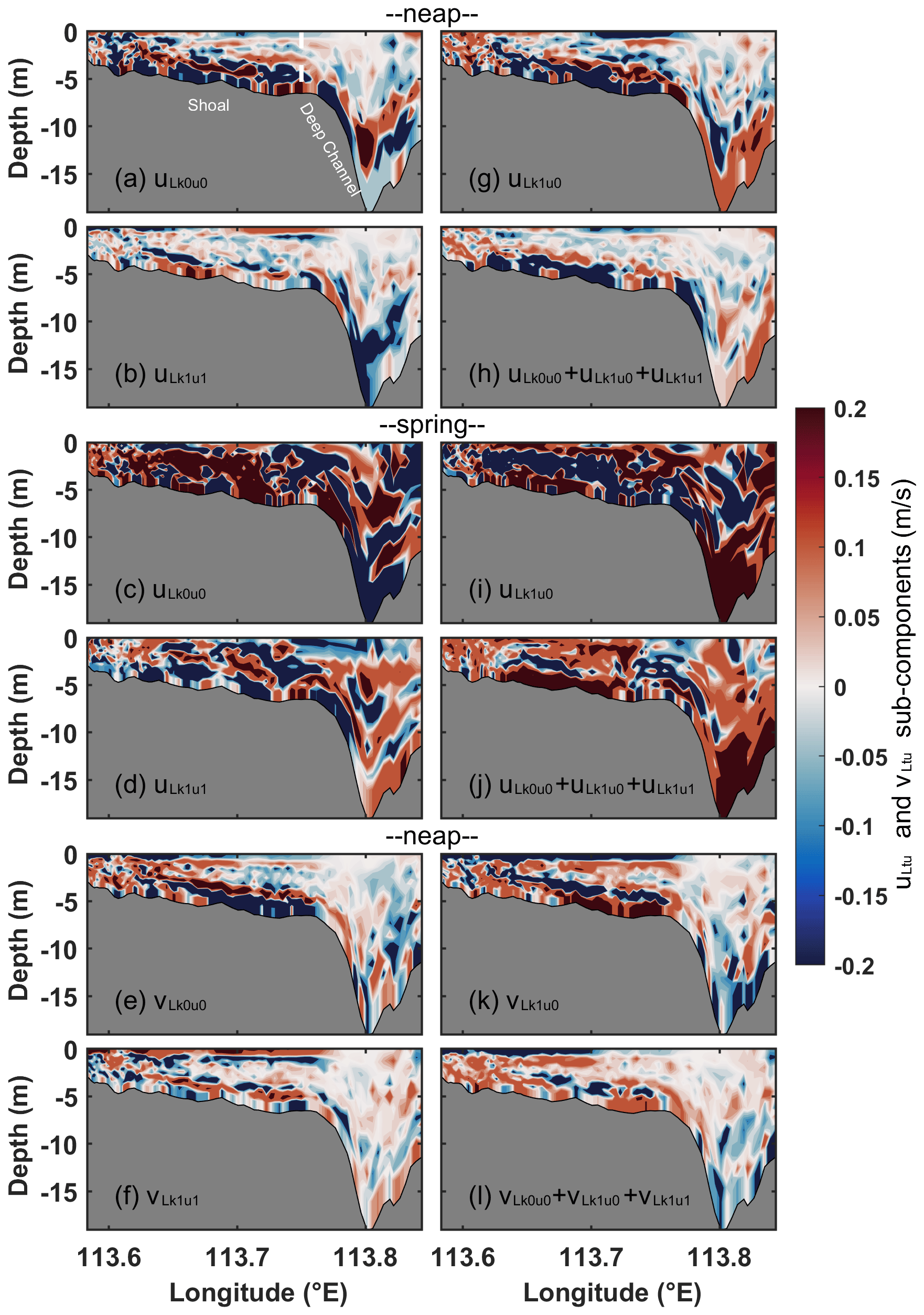
Figure 13 Vertical profiles of non-dominant subcomponents of cross-estuary (u_Ltu) and along-estuary (v_Ltu) eddy viscosity components for Case 1. For cross-estuary subcomponents, (a, c) coupled component of the tidal-averaged eddy viscosity and velocity gradient oscillation (u_Lk0u0), (g, i) tidal straining component (u_Lk1u0), (b, d) coupled component of eddy viscosity oscillation and the tidal-averaged velocity gradient (u_Lk1u1), (h, j) the sum of the three subcomponents during neap (a, b, g, h) and spring (c, d, i, j) tides. (e, k, f, l) Corresponding along-estuary eddy viscosity subcomponents during neap tides.

During neap tides, the along-estuary coupled component of the tidal-averaged eddy viscosity and velocity gradient oscillation (v_Lk0u0) exhibits a vertically sheared structure with alternating outflow and inflow in Case 1 (Fig. 13e). The structure of the along-estuary tidal straining component (v_Lk1u0) closely resembles that of v_Lk0u0 in the upper layer of the shoal, while it is opposite in the lower layer of the shoal and deep channel (Fig. 13k). Additionally, the cross-estuary coupled component of the eddy viscosity oscillation and the tidal-averaged velocity gradient (v_Lk1u1) displays an opposite pattern to v_Lk0u0 in the upper layer of the shoal (Fig. 13f). The combined effects of the three along-estuary non-dominant components (Fig. 13l) are opposite to the dominant component (v_Lk0u1; Fig. 11i) and exert a negative contribution to the total eddy viscosity component (Fig. 11c).

Without the wind forcing, the structures of the non-dominant components of the eddy viscosity component in Case 2 remain consistent with those in Case 1 throughout the entire cross section (not shown). However, during neap tides, their magnitudes in the upper layer manifest a reduction by an order of magnitude relative to Case 1. This indicates a substantial influence of wind on these subcomponents during relatively small tides. During spring tides, both the structure and magnitude (Table 2) of each non-dominant component of the eddy viscosity component align with those in Case 1. This suggests a weak influence of wind on the non-dominant components during spring tides.

When stratification is further ignored in Case 3, the cross-estuary coupled component of the tidal-averaged eddy viscosity and velocity gradient oscillation (u_Lk0u0) exhibits eastward flow in the shoal and the lower layer of the deep channel while displaying westward flow in the upper layer of the deep channel during neap tides (Fig. 14a). This structure differs from that in Case 2, and the magnitude of u_Lk0u0 is approximately 140 times smaller than that in Case 2 (Table 2) during neap tides. The cross-estuary turbulent mean component (u_Lk0u1) for Case 3 predominantly flows westward in most of the shoal and eastward in most of the deep channel (Fig. 14b). The u_Lk0u1 transitions from westward flow in Case 2 to eastward flow in Case 3 in the lower layer of the deep channel. Furthermore, the magnitude of u_Lk0u1 in Case 3 is approximately 12 times smaller than that during neap tides in Case 2. During spring tides, the area of eastward flow of u_Lk0u0 in the shoal is larger than that observed during neap tides in Case 3 (Fig. 14g), and its magnitude is approximately 6 times smaller than that in Case 2. The structure of u_Lk0u1 during spring tides aligns with that observed during neap tides (Fig. 14h), while its magnitude is roughly 20 times smaller than that in Case 2. The magnitude of the cross-estuary coupled component of eddy viscosity oscillation and tidal-averaged velocity gradient (u_Lk1u1) (Fig. 14c and i) in Case 3 is the smallest among the components (Table 2), approximately ranging from 40 to 50 times smaller than that in Case 2.

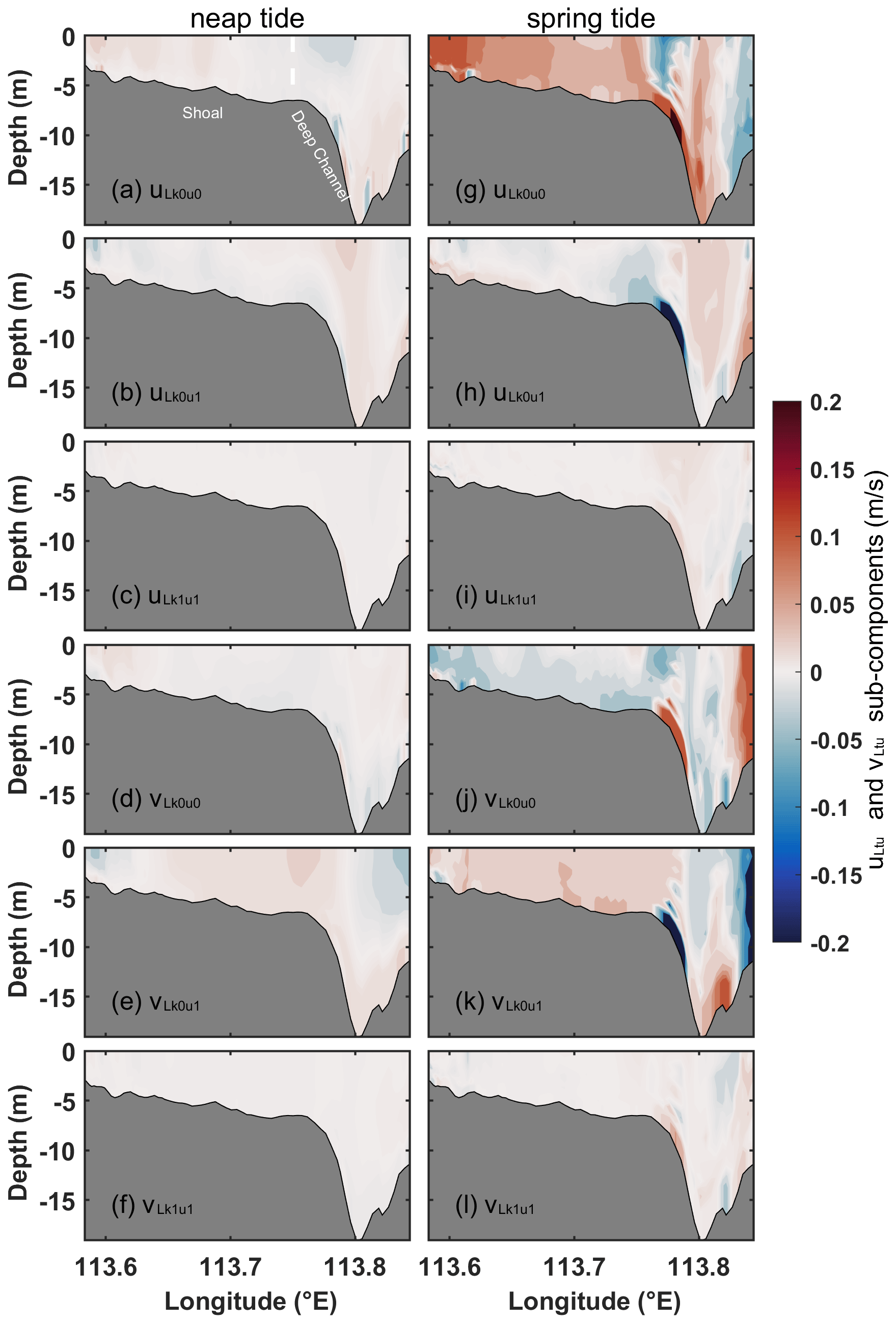
Figure 14 Vertical profiles of non-dominant subcomponents of cross-estuary (u_Ltu) and along-estuary (v_Ltu) eddy viscosity components for Case 3. For cross-estuary subcomponents, (a, g) coupled component of the tidal-averaged eddy viscosity and velocity gradient oscillation (u_Lk0u0), (b, h) turbulent mean component (u_Lk0u1), and (c, i) coupled component of eddy viscosity oscillation and the tidal-averaged velocity gradient (u_Lk1u1) during neap (a–c) and spring (g–i) tides. (d, j, e, k, f, l) Corresponding along-estuary eddy viscosity subcomponents.

The along-estuary non-dominant eddy viscosity subcomponents for Case 3 are depicted in Fig. 14d–f and j–l. During neap tides, both the along-estuary coupled component of the tidal-averaged eddy viscosity and velocity gradient oscillation (v_Lk0u0) and the along-estuary coupled component of eddy viscosity oscillation and tidal-averaged velocity gradient (v_Lk1u1) exhibit horizontally sheared structures (Fig. 14d and f) that differ from those in Case 2. The magnitudes of v_Lk0u0 and v_Lk1u1 are approximately 22–50 times smaller than those in Case 2 (Table 2). During spring tides, the structures of v_Lk0u0 and v_Lk1u1 (Fig. 14j and l) are relatively similar to those during neap tides, and their magnitudes are approximately 12–32 times smaller compared to Case 2. During neap tides, the along-estuary turbulent mean component (v_Lk0u1) for Case 3 displays inflow in the shoal and the lower layer of the deep channel, as well as outflow in the upper layer of the deep channel (Fig. 14e). This pattern is opposite to that in Case 2, and the magnitude of v_Lk0u1 is approximately 6 times smaller than that in Case 2. During spring tides, the outflow area of v_Lk0u1 for Case 3 in the deep channel is larger than that during neap tides (Fig. 14k), and the magnitude is approximately 5 times smaller than that in Case 2. The results elucidate the substantial effect of stratification on each non-dominant component of the eddy viscosity due to the differentially sheared structure, with magnitudes an order greater than in non-stratified scenarios.

4 Discussion

Several dimensionless parameters are examined to quantify the relative impact of the two distinct forcings. The Pearl River Estuary (PRE) features a relatively wide expanse, measuring 20–60 km in width in the middle and lower regions, away from the river discharge input nodes, and extending over a length of 70 km. The Rossby number is approximately 0.2 in the PRE, similar to that calculated by Li et al. (2023), signifying the prominence of the Coriolis force in the region's dynamics. The baroclinic Rossby deformation radius is estimated to be approximately 12–16 km, a range similar to the findings of Pan et al. (2014), suggesting the necessity to account for the rotational effect of the Earth. Lai et al. (2018) highlighted that the influence of the Coriolis force in the PRE is substantial with its effect extending to the bottom layer when compared to vertical mixing and baroclinic and barotropic momentum when analyzing the Eulerian-averaged momentum equation. Chen et al. (2019) indicated that in the depth-integrated momentum balance prior to a storm in the PRE, local momentum balance primarily involves the pressure gradient force, the Coriolis force, and bottom stress. Synthesizing current and prior research, it becomes apparent that the Coriolis force is a predominant factor influencing the dynamics of the PRE. This assertion is corroborated by Wu et al. (2018), who contend that the decomposition approach to Eulerian residual transport assumes particular significance in scenarios marked by a notable presence of Coriolis forces, as evidenced by a small Rossby number. The aforementioned discussion accentuates the criticality and practicality of employing decomposition methods in such analytical contexts.

The Peclet number (Pe), defined as $u_c{L}_c/{\mathit{\upsilon }}_{\mathrm{Dc}}$, measures the relative contribution between the nonlinear advection and horizontal diffusion, where u_c, L_c, and υ_Dc are the scales of tidal current, the estuary length, and the horizontal diffusion coefficient. The Pe for the PRE domain is several orders of magnitude larger than 1, indicating horizontal diffusion is so small that it can be ignored. The results in the paper have indicated that the contribution of the horizontal diffusion component is several-fold lower, or even an order of magnitude, less than other components. Among all terms, the barotropic pressure gradient has the largest scale, making the barotropic pressure gradient component of LRV contribute the most compared to other components. The Wedderburn number (W) is calculated to measure the contribution ratio of wind forcing to the baroclinic pressure gradient, defined as $W=L_c{T}_w/\left(g\mathrm{\Delta }\mathit{\rho }{H}_c^{\mathrm{2}}\right)$ (Lange and Burchard, 2019). The value of W in the PRE is 0.0294 during neap tides and 0.0447 during spring tides, suggesting the baroclinic effects dominate in periodically stratified waters and small W inhibits along-estuary gravitational circulation, which is identical to that in Lange and Burchard (2019). The Simpson number (Si) is a parameter used to quantify the level of stratification in estuaries (Simpson et al., 1990). It is calculated using the following formula:

$$\begin{array}{}\text{(8)}& \mathit{Si}={\displaystyle \frac{{\partial }_{x}b{H}^{\mathrm{2}}}{u_{\max }^{\mathrm{2}}}},\end{array}$$

where ∂_xb represents the tidal mean horizontal density gradient, H represents the water depth, and u_max represents the absolute magnitude of the velocity amplitude. Based on the Simpson number values, different stratification conditions can be determined for the estuary. The estuary is categorized as well-mixed when Si < 0.088. In the case of 0.088 < Si < 0.84, the estuary displays periodic stratification. For Si > 0.84, the estuary is strongly stratified, as indicated by Becherer et al. (2011). The Si for the PRE ranges from 0.1 to 0.45 in stratified conditions in Cases 1 and 2, indicating that the estuary is periodically stratified. Sections B–D are arranged in a north-to-south distribution, gradually approaching the open sea. The Si progressively increases towards the open sea, with values ranging from 0.1 to 0.4 during neap tides and 0.05 to 0.1 during spring tides. This indicates that the magnitude of tides has substantial influences on Si. With the increment in Si, the relative contributions of the tidal straining component and the baroclinic pressure gradient component diminish. These findings align with those of Cheng et al. (2011). Forced by wind, the relative contribution of the two components changes from 2 to 0.57 during neap tides and 2 to 1.4 during spring tides. However, in the absence of wind, the relative contribution varies from 0.67 to 0.26 during neap tides and 1.4 to 0.9 during spring tides, where the value of Si closely mirrors those with wind forcing. The findings underscore that the southwesterly wind amplifies the relative contribution ratios of the tidal straining component to the baroclinic pressure gradient component of the LRV. Specifically, these ratios are 1.5 to 3 times greater compared to scenarios without wind forcing.

According to the Eulerian mean theory, the coupled component of tidal-averaged eddy viscosity and velocity gradient oscillation (u_Ek0u0) and the coupled component of tidal-averaged velocity gradient and eddy viscosity oscillation (u_Ek1u1) are zero (Burchard and Hetland, 2010); however, in the Lagrangian mean theory, those components are not zero, and their magnitudes are comparable to other components under most conditions. Although the tidal straining component of ERV has been extensively discussed, the contribution of the turbulent mean term to the total ERV has not been analyzed in previous studies (Burchard and Hetland, 2010; Burchard et al., 2011). This paper reveals that under stratified conditions, the tidal mean component dominates the eddy viscosity component, even though the magnitudes of tidal straining and the combined component of tidal-averaged eddy viscosity and velocity gradient oscillation are greater than the turbulent mean component. However, these two components exhibit inverse structures of equal magnitude. As a result, their collective impact on the total eddy viscosity component is minimal or negative. Under homogeneous conditions, the tidal straining component dictates the structure of the eddy viscosity. Similarly, the cumulative effects of other components contribute negatively and minimally.

The decomposition methodologies present distinct advantages for elucidating the dynamics of Lagrangian residual velocity (LRV) within generally or weakly nonlinear systems. This significance stems from the absence of comprehensive analytical solutions and definitive governing equations for LRV in generally nonlinear systems, coupled with the constraints of analytical solutions in weakly nonlinear frameworks (Jiang and Feng, 2014; Cui et al., 2019; Chen et al., 2020). In scenarios where the Coriolis force is negligible, the Lagrangian mean momentum equations remain applicable for primary momentum balance analysis. However, these equations are inadequate for the detailed dissection of each LRV component. Notably, in circumstances where the Coriolis effect is minimally impactful, the methodologies employed for LRV decomposition may demonstrate variability, contingent upon the dominant momentum balances. This underscores the necessity for expanded investigation in future scholarly endeavors.

The relevance of the Lagrangian residual circulation for mass transport in estuaries or bays is evident. In the Eulerian-averaged salinity balance equation, a tidal dispersion term emerges (Hansen and Rattray, 1965). This tidal dispersion term exhibits different dynamic mechanisms in various estuaries (Fischer, 1979) and even within different sections of the same estuary. However, when the isohaline averaging method is employed to quantitatively assess estuarine circulation, the tidal dispersion term vanishes (MacCready, 2011; Wang et al., 2017; MacCready et al., 2018). Nevertheless, the salinity coordinate method is only an approximate Lagrangian approach. Future studies focusing on the dynamic mechanisms of salinity transport from a Lagrangian averaging perspective will provide further insights into the subject.

5 Conclusions

The FVCOM model is employed to investigate the dynamic mechanism of the LRV in the PRE. By quantitatively analyzing the contribution of each dynamic component to the LRV, the primary mechanisms governing the LRV in the PRE under conditions of stratification and wind are elucidated, which has been not extensively explored in prior studies (Chu et al., 2022; Deng et al., 2022). Moreover, to discern the impact of the eddy viscosity component on the LRV, this component is decomposed into four subcomponents, with each subcomponent's contribution being quantitatively evaluated. Notably, the decomposition methodologies rooted in Lagrangian theory adopted in this work differ from earlier studies anchored in Eulerian theory (e.g., Burchard et al., 2011; Cheng et al., 2011; Wei et al., 2021). This analysis reveals the prevailing mechanisms shaping the structure of the eddy viscosity component across different dynamic scenarios.

While many studies have focused on ERV in the PRE (e.g., Lai et al., 2018; Xu et al., 2021; Hong et al., 2022), research on LRV in the PRE remains limited, particularly regarding the dynamic mechanisms of LRV. In the reference case, the cross-estuary LRV (u_L) exhibits a two-layer vertical structure with eastward flow in the upper layer and westward flow in the lower layer. The two-layer structure is primarily determined by the combined effects of the eddy viscosity component (u_Ltu), the barotropic pressure gradient component (u_Lba), and the baroclinic pressure gradient component (u_Lgr). The u_Ltu is the main contributor to the eastward flow in the upper layer of the shoal, and u_Lba determines the eastward flow in the upper layer of the deep channel. For the entire lower layer, the westward flow is dominated by u_Ltu and u_Lba, with u_Lgr playing a balancing role. The along-estuary LRV (v_L) exhibits a two-layer gravitational circulation pattern. The v_L is predominantly influenced by the imbalance of the barotropic pressure gradient component (v_Lba) and the baroclinic pressure gradient component (v_Lgr). The outflow is mainly dominated by v_Lba in the upper layer, while the inflow is primarily driven by v_Lgr in the lower layer. For non-dominant components, the combined effects of the local acceleration component and the horizontal and vertical nonlinear component contribute less to total LRV. The contribution of the horizontal diffusion component is negligible.

Without wind forcing, the eastward flow dominated by the eddy viscosity component (u_Ltu) transforms into the westward flow dominated by the barotropic pressure gradient component (u_Lba) in the upper 2 m of the shoal. In other regions, the dominant components of the cross-estuary LRV (u_L) roughly remain the same as those in the reference case, indicating that wind mainly affects u_L in the upper layer by influencing u_Ltu. The structure and dominant components of the along-estuary LRV (v_L) are nearly consistent with those in the reference case except for some regions in the shoal, but the magnitude of the dominant components is larger than that in the reference case, indicating that the southwesterly wind inhibits the along-estuary gravitational circulation. The along-estuary non-dominant components exhibit consistent magnitudes and structures, irrespective of the presence or absence of wind forcing, except for the along-estuary eddy viscosity component, which exhibits a reverse structure in the upper layer compared to that with wind forcing.

Under unstratified conditions, the cross-estuary and along-estuary LRVs (u_L, v_L) are transformed from the vertical shear structure in stratified waters to the lateral shear structure. The u_L is dominated by the sum of the local acceleration component (u_Lac), horizontal nonlinear component (u_Ladh), barotropic pressure gradient component (u_Lba), and eddy viscosity component (u_Ltu). The v_L is dominated by the sum of the barotropic pressure gradient component (v_Lba) and eddy viscosity component (v_Ltu). These results indicate that stratification modulates the structure of the LRV by impacting its dominant components when contrasted with conditions in homogeneous waters.

This study highlights that the eddy viscosity component remains dominant regardless of the presence of stratification. Specifically, under stratified conditions, the turbulent mean component plays a dominant role in the total eddy viscosity component, which has not yet been studied in previous works (e.g., Burchard et al., 2023). Conversely, under unstratified conditions, the tidal straining component takes precedence over other factors in contributing to the total eddy viscosity component, and its magnitude is either several times or 1 order of magnitude bigger than the other components. The combined effects of non-dominant components have a negative contribution to the total eddy viscosity component.

Appendix A: Numerical solutions of each component of the Lagrangian residual velocity (LRV)

Each term in the momentum equations is integrated along the particle trajectories over a tidal period and divided by the tidal period to obtain each dynamic component of Lagrangian residual velocity.

$$\begin{array}{}\text{(A1)}& {\displaystyle }\begin{array}{rl}{v}_{\mathrm{L}}& =\langle \underset{\mathrm{1}}{\underbrace{{\displaystyle \frac{\partial uD}{D\partial t}}\rangle /f}}+\underset{\mathrm{2}}{\underbrace{\langle {\displaystyle \frac{\partial u^{\mathrm{2}}D}{D\partial x}}+{\displaystyle \frac{\partial uvD}{D\partial y}}\rangle /f}}\\ & +\underset{\mathrm{3}}{\underbrace{\langle {\displaystyle \frac{\partial u\mathit{\omega }D}{D\partial \mathit{\sigma }}}\rangle /f}}+\underset{\mathrm{4}}{\underbrace{\langle g{\displaystyle \frac{\partial \mathit{\zeta }}{\partial x}}\rangle /f}}\underset{\mathrm{5}}{\underbrace{-\langle {\displaystyle \frac{\mathrm{1}}{D^{\mathrm{2}}}}{\displaystyle \frac{\partial }{\partial \mathit{\sigma }}}\left(v_h{\displaystyle \frac{\partial u}{\partial \mathit{\sigma }}}\right)\rangle /f}}\\ & +\underset{\mathrm{6}}{\underbrace{\langle {\displaystyle \frac{g}{{\mathit{\rho }}_{\mathrm{0}}}}(D{\int }_{\mathit{\sigma }}^{\mathrm{0}}{\displaystyle \frac{\partial \mathit{\rho }}{\partial x}}\mathrm{d}{\mathit{\sigma }}_{\mathrm{1}}-{\displaystyle \frac{\partial D}{\partial x}}{\int }_{\mathit{\sigma }}^{\mathrm{0}}{\mathit{\sigma }}_{\mathrm{1}}{\displaystyle \frac{\partial \mathit{\rho }}{\partial {\mathit{\sigma }}_{\mathrm{1}}}}\mathrm{d}{\mathit{\sigma }}_{\mathrm{1}})\rangle /f}}\\ & \underset{\mathrm{7}}{\underbrace{-\langle F_x\rangle /f}},\end{array}\text{(A2)}& {\displaystyle }\begin{array}{rl}{u}_{\mathrm{L}}& =\underset{\mathrm{1}}{\underbrace{-\langle {\displaystyle \frac{\partial vD}{D\partial t}}\rangle /f}}\underset{\mathrm{2}}{\underbrace{-\langle ({\displaystyle \frac{\partial uvD}{D\partial x}}+{\displaystyle \frac{\partial v^{\mathrm{2}}D}{D\partial y}})\rangle /f}}\\ & \underset{\mathrm{3}}{\underbrace{-\langle \left({\displaystyle \frac{\partial v\mathit{\omega }D}{D\partial \mathit{\sigma }}}\right)\rangle /f}}\underset{\mathrm{4}}{\underbrace{-\langle g{\displaystyle \frac{\partial \mathit{\zeta }}{\partial y}}\rangle /f}}\underset{\mathrm{5}}{\underbrace{+\langle {\displaystyle \frac{\mathrm{1}}{D^{\mathrm{2}}}}{\displaystyle \frac{\partial }{\partial \mathit{\sigma }}}\left(v_h{\displaystyle \frac{\partial v}{\partial \mathit{\sigma }}}\right)\rangle /f}}\\ & \underset{\mathrm{6}}{\underbrace{-\langle {\displaystyle \frac{g}{{\mathit{\rho }}_{\mathrm{0}}}}(D{\int }_{\mathit{\rho }}^{\mathrm{0}}{\displaystyle \frac{\partial \mathit{\rho }}{\partial y}}\mathrm{d}{\mathit{\sigma }}_{\mathrm{1}}-{\displaystyle \frac{\partial D}{\partial y}}{\int }_{\mathit{\sigma }}^{\mathrm{0}}{\mathit{\sigma }}_{\mathrm{1}}{\displaystyle \frac{\partial \mathit{\rho }}{\partial {\mathit{\sigma }}_{\mathrm{1}}}}\mathrm{d}{\mathit{\sigma }}_{\mathrm{1}})\rangle /f}}\\ & +\underset{\mathrm{7}}{\underbrace{\langle F_y\rangle /f}},\end{array}\end{array}$$

where u (x, y, σ, t), v (x, y, σ, t), and ω (x, y, σ, t) represent velocity components in the longitudinal (x), latitudinal (y), and vertical (σ) directions, respectively. The ρ (x, y, σ, t) is water density, ρ₀ is the reference density, t is the time, f is the Coriolis parameter, and v_h (x, y, σ, t) is the eddy viscosity coefficient. $D=H+\mathit{\zeta }$, where H(x, y) is the water mean depth and ζ (x, y, t) is the water surface elevation. The first term refers to the local acceleration component, the second terms represent horizontal nonlinear advection components, the third term depicts the nonlinear vertical advection component, the fourth term corresponds to the barotropic pressure gradient component, the fifth term describes the eddy viscosity component, the sixth terms denote the baroclinic pressure gradient components, and the seventh term pertains to the horizontal diffusion component. The < > denotes the Lagrangian mean operator.