Dependency of simulated tropical Atlantic current variability on the wind forcing

The upper wind-driven circulation in the tropical Atlantic Ocean plays a key role in the basin-wide distribution of water mass properties and affects the transport of heat, freshwater, and biogeochemical tracers such as oxygen or nutrients. It is crucial to improve our understanding of its long-term behaviour, which largely relies on model simulations and applied forcing due to sparse observational data coverage, especially before the mid-2000s. Here, we apply two different forcing products, the Coordinated Ocean-ice Reference Experiments (CORE) v2 and the Japanese 55-year Reanalysis (JRA55-do) surface dataset, to a high-resolution ocean model. Where possible, we compare the simulated results to long-term observations. We find large discrepancies between the two simulations regarding the wind and current field. In the CORE simulation, strong, large-scale wind stress curl amplitudes above the upwelling regions of the eastern tropical North Atlantic seem to cause an overestimation of the mean and seasonal variability in the eastward subsurface current just north of the Equator. The wind stress curl of JRA55-do forcing shows much finer structures, and the JRA55-do simulation is in better agreement with the mean and intraseasonal fluctuations in the subsurface current found in observations. The northern branch of the South Equatorial Current flows westward at the surface just north of the Equator. On interannual to decadal timescales, it shows a high correlation of R=0.9 with the zonal wind stress in the CORE simulation but only a weak correlation of R=0.35 in the JRA55-do simulation. We also identify similarities between the two simulations. The strength of the eastward-flowing North Equatorial Counter Current located between 3 and 10° N covaries with the strength of the meridional wind stress just north of the Equator on interannual to decadal timescales in the two simulations. Both simulations present a comparable mean, seasonal cycle and trend of the eastward off-equatorial subsurface current south of the Equator but underestimate the current strength by half compared to observations. In both simulations, the eastward-flowing Equatorial Undercurrent weakened between 1990 and 2009. In the JRA simulation, which covers the modern period of observations, the Equatorial Undercurrent strengthened again between 2008 to 2018, which agrees with observations, although the simulation underestimates the strengthening by over a third. We propose that long-term observations, once they have reached a critical length, need to be used to test the quality of wind-driven simulations. This study presents one step in this direction.

1 Introduction

The tropical Atlantic circulation plays a crucial role in the distribution of heat, freshwater, carbon and ecosystem-relevant quantities in the Atlantic Ocean. A unique feature of the Atlantic Ocean is the Atlantic meridional overturning circulation (AMOC). The return flow of the AMOC in the upper ocean transports heat freshwater and biogeochemical properties like carbon or oxygen northward through the basin, impacting climate and ecosystems in the entire Atlantic sector. On their way through the tropics, water masses experience an important transformation, gaining heat (0.22 PW; Hazeleger and Drijfhout, 2006) and salinity (freshwater divergence of 0.16 Sv; Hazeleger and Drijfhout, 2006). About one-third of the northward flow is recirculated within the tropical Atlantic current system (Hazeleger and Drijfhout, 2006; Tuchen et al., 2022a). While observations now allow the description of the mean to sub-decadal variability in the upper tropical Atlantic circulation (e.g. Tuchen et al., 2022a; Brandt et al., 2021; Burmeister et al., 2020), the study of decadal changes and trends largely relies on model output (e.g. Burmeister et al., 2019; Hüttl-Kabus and Böning, 2008; Duteil et al., 2014).

The flow field in the tropical Atlantic represents a superposition of shallow meridional overturning cells, the horizontal wind-driven gyre circulation and the basin-wide AMOC (e.g. Schott et al., 2004; Hazeleger and Drijfhout, 2006; Perez et al., 2014; Tuchen et al., 2022a; Heukamp et al., 2022). The currents are thus a result of the easterly trade winds and the resultant equatorial Ekman divergence, the wind stress curl fields in the tropics and subtropics, as well as buoyancy and wind forcing at higher latitudes. In the upper ∼300 m, the shallow subtropical cells (STCs) consist of poleward Ekman transport at the surface and equatorward transport in the thermocline, which connect the subduction regimes in the subtropics and the upwelling regimes in the tropics (Schott et al., 2004). Upwelling in the tropical Atlantic occurs along the Equator, east of about 20° W, within the Guinea and Angola domes and within the eastern boundary upwelling systems off the coast of West Africa. The strength of the STCs is related to the equatorial Ekman divergence (Tuchen et al., 2019; Rabe et al., 2008) and can impact the strength of the zonal currents in the tropical Atlantic, especially the Equatorial Undercurrent (EUC; Rabe et al., 2008; Brandt et al., 2021). The tropical overturning cells (TCs) are part of the STCs and dominate the meridional flow field in the upper 100 m between 5° N and 5° S (e.g. McCreary and Lu, 1994; Schott et al., 2004; Molinari et al., 2003; Perez et al., 2014). They are governed by wind-driven equatorial upwelling, poleward Ekman transport in the upper limb, off-equatorial downwelling at about ±3–5° latitude and a geostrophic flow directed equatorward in the lower limb (e.g. Perez et al., 2014). The shallowest overturning cell is the equatorial roll in the upper 80 m along the Equator. The southerly wind stress at the Equator drives its northward cross-equatorial flow near the surface and southward flow below (Heukamp et al., 2022). A complex system of alternating eastward and westward narrow current bands and strong western boundary currents with northward flow participates in or is superimposed on the STCs, TCs and the equatorial roll (e.g. Schott et al., 2004).

The wind-driven gyre circulation in the tropical Atlantic can be largely explained by Sverdrup dynamics; that is the relationship between wind stress curl and depth-integrated meridional transport. The trade winds converge in the Intertropical Convergence Zone (ITCZ) slightly north of the Equator. The weakening of the north- and southeasterly trade winds towards the ITCZ is associated with a positive and negative wind stress curl north and south of the ITCZ, respectively. According to the Sverdrup dynamics, this results in two wind-driven gyres, the tropical gyre north and the equatorial gyre south of the ITCZ (e.g. Fratantoni et al., 2000). Below the ITCZ, an eastward-flowing geostrophic current exists between 3 and 13° N, which is the North Equatorial Counter Current (Fig. 1; Urbano et al., 2006). In the north and in the south, it is flanked by the westward-flowing North Equatorial Current (NEC) and South Equatorial Current (SEC), respectively. Associated with the northward displacement of the ITCZ, the SEC reaches into the Northern Hemisphere, and the literature often distinguishes between a southern branch (sSEC; south of 10° S), a central branch (cSEC; south of the Equator) and a northern branch (nSEC; centred at about 2° N) (e.g. Peterson and Stramma, 1991; Schott et al., 2004).

Persistent easterly winds along the Equator push the surface waters towards the west, causing the thermocline to slope upwards to the east and hence driving, amongst other factors, the eastward-flowing subsurface EUC along the Equator (Pedlosky, 1987; Wacongne, 1989). The EUC supplies water masses from the western basin, mostly of southern subtropical origin, towards the central and eastern upwelling regions (e.g. Bourlès et al., 2002; Schott et al., 2004; Brandt et al., 2006). Two off-equatorial eastward-flowing subsurface currents exist in the Atlantic, namely the North Equatorial Undercurrent (NEUC) and the South Equatorial Undercurrent (SEUC) centred at about 5° N/S, respectively. Potential driving mechanisms of the NEUC and SEUC are still not fully understood. Assene et al. (2020) investigated the formation and maintenance of the off-equatorial subsurface currents in the Gulf of Guinea and highlighted the link between submesoscale processes, mesoscale vortices and mean currents, which can include any of the driving mechanisms suggested in previous studies, namely eddy fluxes (Jochum and Malanotte-Rizzoli, 2004), meridional advection (Wang, 2005; Johnson and Moore, 1997; Marin et al., 2000; Hua et al., 2003; Marin et al., 2003; Ishida et al., 2005), lateral diffusion of vorticity (McPhaden, 1984) and the pull by upwelling in the eastern basin (McCreary et al., 2002; Furue et al., 2007, 2009). Please note that some of these studies focus on the Pacific counterparts of the NEUC and SEUC; due to the resemblance of the equatorial Atlantic and Pacific zonal current structure (e.g. Schott et al., 2004), processes observed in the Pacific off-equatorial undercurrents are thought to also apply in the Atlantic (Assene et al., 2020).

The zonal currents in the tropical Atlantic (Fig. 1) form an interhemispheric buffer for the AMOC. A quantification of the different AMOC pathways in the tropical Atlantic was done by Tuchen et al. (2022a). The main part of the upper AMOC limb enters the tropical Atlantic within the westward-flowing sSEC that bifurcates into the northward-flowing North Brazil Undercurrent (NBUC) and the southward-flowing Brazil Current at about 15° S. The NBUC merges with the cSEC north of about 5° S, and the northward western boundary current becomes a surface-intensified current and is called the North Brazil Current (NBC). Within the NBC, the AMOC finally crosses the Equator (e.g. Schott et al., 2004; Hazeleger and Drijfhout, 2006; Rühs et al., 2015). After overshooting the Equator, the NBC partly retroflects into the zonal current field and partly breaks up into northward-propagating NBC rings (Johns et al., 2003). The EUC, NEUC and North Equatorial Counter Current (NECC) feed on the retroflection of the NBC (Bourlès et al., 1999; Hüttl-Kabus and Böning, 2008; Rosell-Fieschi et al., 2015; Stramma et al., 2005). Furthermore, the NEUC and NECC are partly supplied by water masses of Northern Hemisphere origin from the retroflection of the westward-flowing North Equatorial Current, which is part of the subtropical gyre in the North Atlantic (e.g. Schott et al., 1998; Bourlès et al., 1999; Urbano et al., 2008). The eastward currents connect the subducted water masses from the subtropical gyres with the central and eastern upwelling regions in the tropical Atlantic, thereby ventilating the oxygen-poor eastern basin (Stramma et al., 2008; Urbano et al., 2008; Hahn et al., 2014; Brandt et al., 2015; Hahn et al., 2017; Burmeister et al., 2019, 2020).

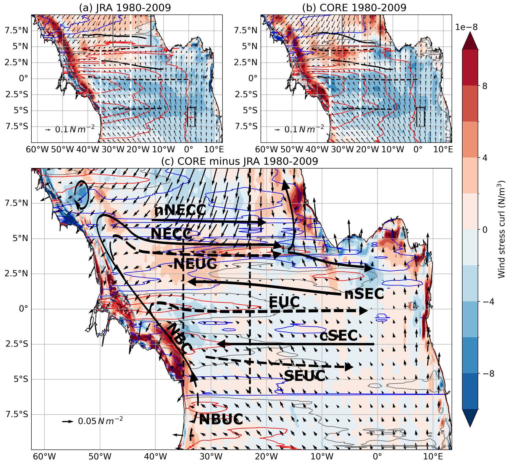
Figure 1 (a–c)The 1980 to 2009 mean maps of wind stress (black arrows), wind stress curl (colour shading) and associated Sverdrup stream function (contour lines) calculated using (a) JRA_sim, (b) CORE_sim and (c) the difference between the two forcings. Blue contour lines show negative values, red contour lines show positive values of Sverdrup stream function, and the zero line is marked as a grey contour. A negative stream function presents an anticlockwise rotation; this means that a zero contour of the stream function with negative values in the south (north) marks the maximum westward (eastward) velocities. In panels (a)–(b), the contour line interval is 2 Sv. In panel (c), the ±1.5 and ±0.5 Sv isolines are shown. Zonal black lines in panels (a) and (b) mark the mean latitude (Y_CM; Eq. 1) of the simulated surface (solid) and subsurface (dashed) currents for the respective periods. Meridional dashed white lines in panels (a) and (b) and dashed black lines in panel (c) mark 35 and 23° W sections. The black rectangles in panels (a) and (b) mark the upwelling regions of the Guinea Dome in the Northern Hemisphere and the Angola Dome in the Southern Hemisphere. (c) Superimposed in black are surface (solid) and thermocline (dashed) currents (adapted from Burmeister et al., 2019, based on observations), including the North Equatorial Counter Current (NECC), northern branch of the NECC (nNECC), North Equatorial Undercurrent (NEUC), northern branch of the South Equatorial Current (nSEC), central branch of the South Equatorial Current (cSEC), Equatorial Undercurrent (EUC), South Equatorial Undercurrent (SEUC), North Brazil Undercurrent (NBUC) and North Brazil Current (NBC).

In the equatorial Atlantic, the enhanced semi-annual to interannual variability in the zonal flow can be attributed to basin resonances of the gravest basin mode (Thierry et al., 2004; Ascani et al., 2006; d'Orgeville et al., 2007; Ding et al., 2009; Greatbatch et al., 2012; Claus et al., 2016; Brandt et al., 2016). Resonant equatorial basin modes are low-frequency standing equatorial modes consisting of long equatorial Kelvin and Rossby waves (Cane and Moore, 1981). Depending on the gravity wave speed and the basin geometry, each baroclinic mode has a characteristic resonance period. The semi-annual and annual zonal flow variability in the equatorial Atlantic is attributed to the gravest basin mode for the second and the fourth baroclinic mode, respectively (Brandt et al., 2016).

A realistic simulation of the narrow zonal current bands and their variability in the tropical Atlantic is still challenging. While climate models are generally too coarse to fully resolve the tropical Atlantic current system, recent high-resolution ocean general circulation models better represent the mean state of the zonal currents (Duteil et al., 2014). Still, distinct discrepancies to ocean observations exist (Burmeister et al., 2020, 2019). Burmeister et al. (2020) showed a relationship between zonal current and wind stress curl variability, suggesting that it is important to resolve fine wind stress curl patterns to simulate the narrow-banded zonal current system in the tropical Atlantic.

In this study, we investigate how two different forcing products with different spatial and temporal resolution impact the mean state and variability in the narrow-banded zonal current system in the tropical Atlantic. The forcing products are the well-established but discontinued Coordinated Ocean-ice Reference Experiments (CORE) v2 (Large and Yeager, 2009) and its successor, the Japanese 55-year Reanalysis (JRA55-do) surface dataset (Tsujino et al., 2018). The simulations are performed with a global ocean model covering the tropical Atlantic Ocean at eddying resolution, INALT20, which has the capability to resolve the complex zonal current system in the tropical Atlantic. Furthermore, we have access to over 10 years of velocity observations, and this period is now covered by JRA55-do forcing. This allows for a direct comparison between model and observations, which is not possible for simulations forced by CORE.

2 Data and methods

In this section, we describe the data and methods used in this paper. In summary, we compare two simulations with a high-resolution global ocean circulation model forced by two different atmospheric products, the Coordinated Ocean-ice Reference Experiments (CORE) v2 dataset (Griffies et al., 2009) and the JRA55-do surface dataset v1.4.1 (Tsujino et al., 2018). We calculate current transport for the eastward-flowing EUC, NEUC, SEUC and NECC and the westward-flowing nSEC, utilising an algorithm which is following the current cores (Hsin and Qiu, 2012; Burmeister et al., 2019). The model results are compared to shipboard hydrographic and velocity observation along 23° W (e.g. Brandt et al., 2015; Hahn et al., 2017; Burmeister et al., 2020) and 35° W (Hormann and Brandt, 2007; Tuchen et al., 2022a), as well as the current transport time series derived from moored observations at 1.2° N to 1.2° S, 23° W (Brandt et al., 2021) and 5° N, 23° W (Burmeister et al., 2020). Furthermore, we perform a modal decomposition of the simulated zonal velocity field and briefly introduce the equations used to calculate the Sverdrup stream function, Ekman transport and an index for the activity of tropical instability waves (Lee et al., 2014; Olivier et al., 2020; Perez et al., 2012; Tuchen et al., 2022b).

2.1 High-resolution global ocean circulation model INALT20

Our analyses are based on 5 d averaged output of the global ocean circulation model INALT20. In INALT20, a $\mathrm{1}/\mathrm{20}$° nest covering the South Atlantic and the western Indian oceans between 70° W and 70° E and the northern tip of the Antarctic Peninsula at 10° N to 63° S is embedded into a global $\mathrm{1}/\mathrm{4}$° host model (Schwarzkopf et al., 2019). The model is based on the Nucleus for European Modelling of the Ocean (NEMO) v3.6 code (Madec and the NEMO team, 2017), incorporating the Louvain-la-Neuve sea ice model version 2 and using a viscous–plastic rheology (LIM2-VP; Fichefet and Maqueda, 1997). A global configuration with tripolar grids, named ORCA025, is used as a host to build the regionally finer-resolved configuration realised by the AGRIF (Adaptive grid refinement in Fortran) library (Debreu et al., 2008). This set up allows two-way interactions, where the host not only provides boundary conditions for the nest but also receives information from the nest.

The model configuration has a vertical grid, with 46 z levels varying in vertical grid size from 6 m at the surface to 250 m in the deepest layers, resolving the first baroclinic mode (Stewart et al., 2017; Schubert et al., 2019), which is needed for the representation of the major baroclinic currents. The same vertical grid has proven to be an appropriate choice for simulations with model configurations up to $\mathrm{1}/\mathrm{20}$° horizontal resolution (e.g. Böning et al., 2016; Behrens et al., 2017). The bottom topography is represented by partial steps (Barnier et al., 2006), with a minimum layer thickness of 25 m.

In this study, we use two hindcast simulations which are forced with two different forcing products for the period 1958 to 2009 and 2019, respectively. The two hindcast simulations are preceded by a 30-year spin-up integration. The spin-up integration is initialised with temperature and salinity from the World Ocean Atlas (Levitus et al., 1998, with modifications in the polar regions from the Polar science center Hydrographic Climatology (PHC); Steele et al., 2001) and an ocean at rest. The spin-up is forced by interannually varying atmospheric boundary conditions from 1980 to 2009, using CORE.

The well-established but discontinued CORE forcing covers the period from 1948 to 2009 (Griffies et al., 2009) and builds on National Centers for Environmental Prediction/National Center for Atmospheric Research (NCEP/NCAR) reanalysis data merged with satellite-based radiation and precipitation, employing a set of parameter corrections to minimise global flux imbalances. Prior to the satellite era, CORE does not contain realistic time-varying radiation and precipitation fluxes, as climatological values are used to fill in missing years (Large and Yeager, 2009). It has a horizontal resolution of 2° × 2° and temporal resolution of 6 h. CORE is limited by the relatively coarse spatial and temporal resolution and was discontinued in 2009; thus it does not cover the most recent decade of observations. Additionally, multidecadal variability in this dataset might be problematic, as it includes NCEP winds known to exhibit spurious multidecadal wind variability (Fiorino, 2000; He et al., 2016; Hurrell and Trenberth, 1998). In the following, we refer to the model simulation forced with the CORE forcing as CORE_sim.

The second forcing product is the more recent JRA55-do surface dataset v1.4.1 (Tsujino et al., 2018), which we refer to as the JRA in the following. It is based on the 55-year reanalysis project (JRA-55; e.g. Kobayashi et al., 2015) conducted by the Japan Meteorological Agency (JMA). This dataset stands out due to its higher horizontal (55 km) and temporal resolution (3 h), which now covers the entire observational period (1958 to 2018). Similar to CORE, the surface fields from an atmospheric reanalysis are adjusted relative to reference datasets. The downwelling radiative fluxes and precipitation are based on reanalysis products in contrast to CORE, which uses satellite observations. In the following, we refer to the simulation forced with JRA as JRA_sim.

2.2 Shipboard observations

The meridional ship sections of velocity, hydrography and oxygen used in this study are an extension of the dataset used by Burmeister et al. (2020). The dataset consists of 31 velocity sections, as well as 22 hydrographic and oxygen sections, which were obtained during cruises along 21 to 28° W between 2000 and 2018 (Table A1). Most sections are along 23° W between 14° N and 6° S and vertically extend from the surface to 600 or 800 m.

Velocity data were acquired by vessel-mounted acoustic Doppler current profilers (vm-ADCPs). The vm-ADCPs continuously record velocities throughout a ship section, and the accuracy of 1 h averaged data is better than 2–4 cm s⁻¹ (Fischer et al., 2003). Hydrographic and oxygen data obtained during conductivity, temperature and depth (CTD) casts were typically taken on a uniform latitude grid with half-degree resolution. The data accuracy for a single research cruise is generally assumed to be better than 0.002 °C, 0.002 and 2 µmol kg⁻¹ for temperature, salinity and dissolved oxygen, respectively (Hahn et al., 2017). The single velocity, hydrographic and oxygen ship sections are mapped on a regular grid (0.05° latitude × 10 m) and are smoothed by a Gaussian filter (horizontal and vertical influence (cutoff) radii at 0.05° (0.1°) latitude and 10 m (20 m), respectively). The single sections are temporally averaged at each grid point to derive mean sections, which are again smoothed by the Gaussian filter.

To derive a second observational estimate for the mean current strength in the western basin, we additionally use 16 velocity and hydrographic ship sections along 35° W from 1990 to 2006 (Table A2). This dataset was used by Hormann and Brandt (2007) and Tuchen et al. (2022a). Note that shipboard velocity observations do not cover the uppermost water layers. This is why all ship sections are limited to the shallowest common water depth, which is 30 m. This is also the upper limit used for any transport estimation of surface currents derived from shipboard observations.

2.3 Path following transport estimation

Transport of the zonal currents at a given longitude in the tropical Atlantic is estimated using the model output and shipboard observations, following the approach of Hsin and Qiu (2012). First the central position Y_CM of the current is estimated using the concept of centre of mass

$$\begin{array}{}\text{(1)}& Y_{\mathrm{CM}}\left(t\right)={\displaystyle \frac{{\int }_{Z_{\mathrm{l}}}^{Z_{\mathrm{u}}}{\int }_{Y_{\mathrm{S}}}^{Y_{\mathrm{N}}}yu(y,z,t)\mathrm{d}y\mathrm{d}z}{{\int }_{Z_{\mathrm{l}}}^{Z_{\mathrm{u}}}{\int }_{Y_{\mathrm{S}}}^{Y_{\mathrm{N}}}u(y,z,t)\mathrm{d}y\mathrm{d}z}},\end{array}$$

where y is latitude, u is zonal velocity, z is depth, t is time, Z_u (Z_l) is the upper (lower) boundary of the flow defined as the depth of specific values of potential density (if not otherwise stated), and Y_N (Y_S) is the northern (southern) limit of the current core.

Now the eastward velocity is integrated within a box, whose meridional range is given by Y_CM(t) and the half-mean width W of the flow, as follows:

$$\begin{array}{}\text{(2)}& \text{INT}\left(t\right)=\underset{Z_{\mathrm{l}}}{\overset{Z_{\mathrm{u}}}{\int }}\underset{Y_{\mathrm{CM}}-W}{\overset{Y_{\mathrm{CM}}+W}{\int }}u(y,z,t)\mathrm{d}y\mathrm{d}z.\end{array}$$

The parameters chosen for each current are listed in Table 1.

Table 1 Parameters for the along-pathway algorithm (Eqs. 1 and 2).

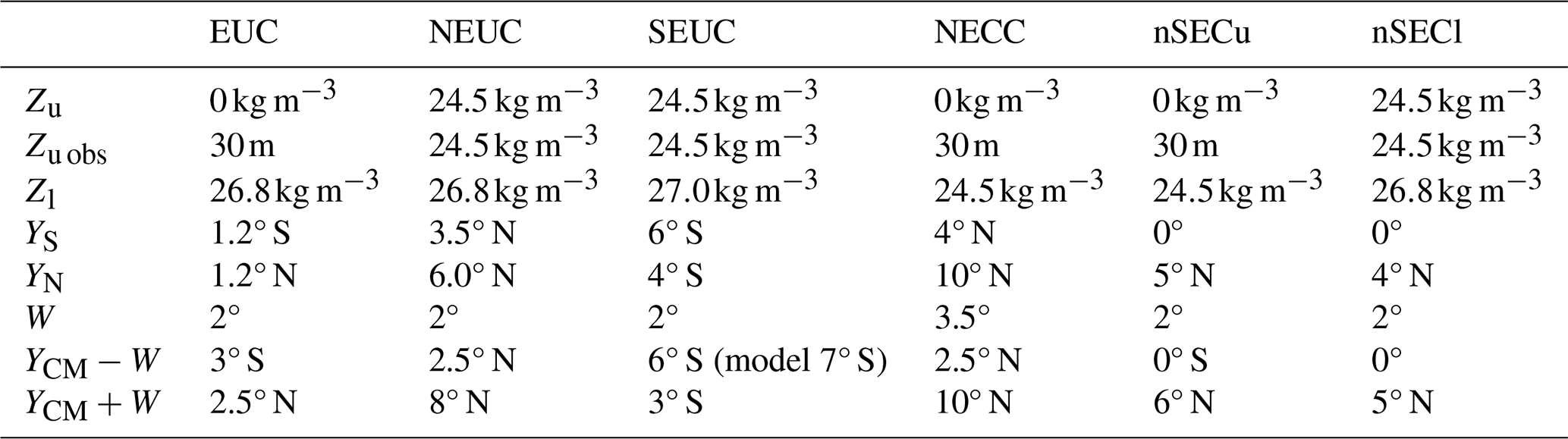
Z_u (Z_l) is the upper (lower) boundary of the flow, which is defined as the depth of the specific values of potential density (if not otherwise stated), and Y_N (Y_S) is the northern (southern) limit of the current core. W is the half-mean width of the current, and Y_CM+W (Y_CM−W) is the northern (southern) absolute limit for the flow integration. Note that as the moored and shipboard observations do not cover the upper water layer, we choose the upper boundary of the flow Z_U obs to be 30 m, which is the shallowest common depth of all observations.

2.4 Moored transport time series

We use long-term observational transport time series estimated for the EUC by Brandt et al. (2021, 2014) and for the NEUC by Burmeister et al. (2020) to validate the model simulations. Transport time series of the EUC and NEUC are reconstructed from moored velocity observations at 0° N, 23° W (May 2005–September 2019) and 5° N, 23° W (July 2006–February 2008 and November 2009–January 2018), respectively.

Horizontal velocity data were acquired using moored ADCPs. At the Equator, the upper water column was observed by one 300 or 150 kHz upward-looking ADCP between 100 and 230 m depth and another 75 kHz ADCP either downward-looking from just below the upper instrument or upward-looking from 600 to 650 m depth. Apart from a period between 2006 and 2008 when the upper instrument failed, the velocity measurements cover the whole depth range of the EUC. At 5° N, either a downward- (July 2006–February 2008) or upward-looking (November 2009–January 2018) 75 kHz ADCP was installed. The upper measurement range of the 5° N ADCPs varies between 65 and 75 m, which means that the upper 10 m of the NEUC is not always covered. This is accounted for in the model-derived transport estimation when compared to the observation. The effect of tides is removed from the moored velocity data by a 40 h low-pass Butterworth filter and subsampling to a regular 12 h time interval. The short-term variability in the tropical Atlantic exceeds the measurement accuracy of the different ADCPs, and errors in the ADCP compass calibrations from different mooring periods are expected to be unsystematic (Brandt et al., 2021).

The EUC transport time series is estimated by regressing spatial variability patterns derived from shipboard observations onto the moored velocity time series at 0° N, 23° W (Brandt et al., 2014, 2016, 2021). Eastward velocities (u>0) of the reconstructed latitude–depth sections (30–300 m depth and 1.2° N–1.2° S latitude) are integrated to obtain the EUC transport. The root mean square differences for the EUC transport reconstruction using equatorial mooring and the transport derived from the shipboard observations is 1.29 Sv (Brandt et al., 2014).

The NEUC transport time series is estimated from shipboard and moored velocity observations, using the optimal width method (Burmeister et al., 2020). First, eastward velocities (u>0) of shipboard observations are latitudinally integrated between 65 and 270 m depth and 4.25 and 5.25° N. To reconstruct the latitudinally integrated velocities (U(z)), an optimal latitude range needs to be found by regressing U(z) onto the shipboard eastward velocity profile at the mooring position. The moored velocity profiles are multiplied by the optimal latitude range (0.88°) and finally depth-integrated to obtain the NEUC transport time series. The root mean square difference in the reconstructed NEUC transport from the shipboard observations is 0.52 Sv (Burmeister et al., 2020).

Note that the reconstructed transport represents the current transport integrated over a fixed box. To compare transport from model output and moored observations at 23° W, we calculate the transport for the EUC and NEUC from model output as the integral of eastward velocity in the respective box (EUC is 30–300 m and 1.2° N–1.2° S; NEUC is 60–270 m and 4.25–5.25° N).

2.5 Modal decomposition

We decompose the velocity field of the two model simulations using vertical structure functions ${\widehat{p}}_n\left(z\right)$ obtained from a mean buoyancy frequency profile derived from observations (Brandt et al., 2016). Following the approach of Claus et al. (2016), we derive ${\widehat{p}}_n\left(z\right)$ from a mean buoyancy frequency profile obtained from 70 shipboard CTD profiles (Table A1). To obtain the mean buoyancy frequency profile, we use CTD profiles with a minimum depth of 1200 m within a 1° wide, squared box centred at 0° N, 23° W. We bin-averaged the individual temperature and salinity profiles to a uniform 10 m vertical grid with a maximum depth of 4500 m and calculated a buoyancy frequency profile for each cast separately; these are then averaged to obtain the mean buoyancy frequency profile. It is important to note that baroclinic modes are only orthogonal if the velocity data are covering the complete upper 4500 m depth. Missing data, as typical of shipboard or moored data, reduce the orthogonality and introduce uncertainties in the calculation. However, consistent results between studies provide some confidence in the chosen approach (e.g. Brandt et al., 2016; Claus et al., 2016; Kopte et al., 2018).

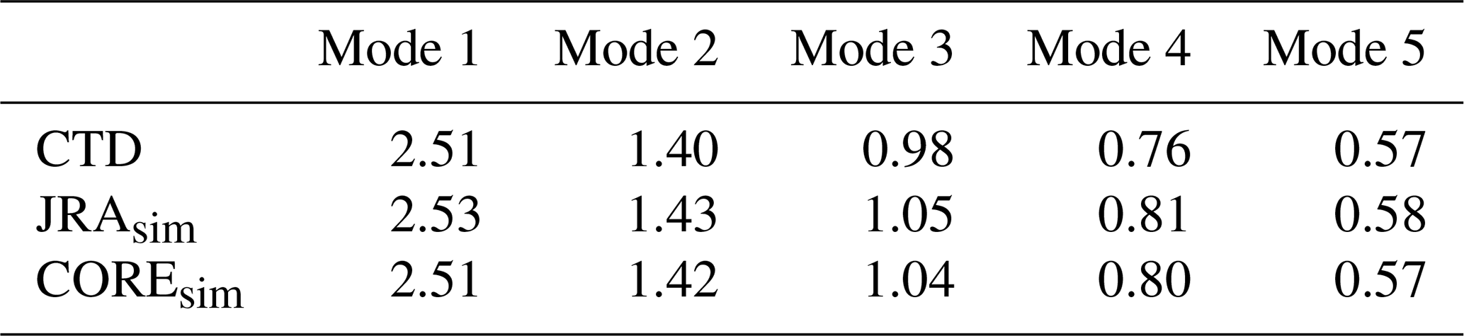
The gravity wave speed of the first five baroclinic modes derived from observations is shown in Table 2. We also derive the vertical structure functions from mean buoyancy frequency profiles using model output from JRA_sim and CORE_sim. For the gravity wave speed, the two simulations are in good agreement with each other and with the observations.

Table 2 Gravity wave speed of the first five baroclinic modes of the gravest basin mode, using squared buoyancy frequencies within a 1° wide, squared box centred at 0° N, 23° W, using CTD profiles and model output from JRA_sim and CORE_sim.

To estimate the contribution of the first five modes to the annual and semi-annual cycle of the zonal velocity field in the tropical Atlantic (10° N–10° S) we use the orthogonality between functions. We fit the vertical normal baroclinic modes and temporal harmonics with reduction operations as follows.

Let ${\widehat{p}}_n\left(z\right)$ be the vertical normal (baroclinic) modes with

$$\begin{array}{}\text{(3)}& \int \mathrm{d}z{\widehat{p}}_n\left(z\right)\cdot {\widehat{p}}_m\left(z\right)={\mathit{\delta }}_{n,m},\end{array}$$

and h_T,τ(t) be the temporal harmonic modes with period T and phase τ, which fulfil

$$\begin{array}{}\text{(4)}& {\displaystyle }\int \mathrm{d}t{h}_{T,\mathrm{0}}\left(t\right)\cdot h_{T/\mathrm{2},\mathrm{0}}\left(t\right)=\mathrm{0}\text{(5)}& {\displaystyle }\int \mathrm{d}t{h}_{T,\mathrm{0}}\left(t\right)\cdot h_{T,\mathrm{0}}\left(t\right)=\mathrm{1}.\end{array}$$

Then, we could compose a signal s(t,z), with different normal modes each having a separate annual and semi-annual cycle as follows:

$$\begin{array}{}\text{(6)}& \begin{array}{rl}s(t,z)& =\sum _n{\mathit{\alpha }}_n^{\mathrm{a}}\cdot {\widehat{p}}_n\left(z\right)\cdot h_{\mathrm{365}\mathrm{d},{\mathit{\tau }}_n^{\mathrm{a}}}\left(t\right)\\ & +\sum _n{\mathit{\alpha }}_n^{\mathrm{s}}\cdot {\widehat{p}}_n\left(z\right)\cdot h_{\mathrm{365}\mathrm{d}/\mathrm{2},{\mathit{\tau }}_n^{\mathrm{s}}}\left(t\right),\end{array}\end{array}$$

where ${\mathit{\alpha }}_n^{\mathrm{a}}$ is the amplitude of the annual cycle of the baroclinic mode n, ${\mathit{\alpha }}_n^{\mathrm{s}}$ is the amplitude of the semi-annual cycle of the baroclinic mode n, ${\mathit{\tau }}_n^{\mathrm{a}}$ is the phase shift in the annual cycle of baroclinic mode n, and ${\mathit{\tau }}_n^{\mathrm{s}}$ is the phase shift in the semi-annual cycle of baroclinic mode n.

The time variability in the baroclinic mode n can be diagnosed using a depth integral

$$\begin{array}{}\text{(7)}& \begin{array}{rl}{\mathit{\alpha }}_n^{\mathrm{a}}\cdot h_{\mathrm{365}\mathrm{d},{\mathit{\tau }}_n^{\mathrm{a}}}\left(t\right)+{\mathit{\alpha }}_n^{\mathrm{a}}\cdot h_{\mathrm{365}\mathrm{d}/\mathrm{2},{\mathit{\tau }}_n^{\mathrm{a}}}\left(t\right)& =\int \mathrm{d}z{b}_n\left(z\right)\cdot s(t,z)\\ & \equiv s_n\left(t\right).\end{array}\end{array}$$

The phase and amplitude of s_n(t) can be diagnosed by projecting a time series covering and integer number of years on a normalised annual ${\mathrm{e}}^{i\mathrm{2}\mathit{\pi }/\mathrm{365}\mathrm{d}\cdot t}$ or semi-annual ${\mathrm{e}}^{i\mathrm{4}\mathit{\pi }/\mathrm{365}\mathrm{d}\cdot t}$:

$$\begin{array}{}\text{(8)}& {\displaystyle }{\mathit{\alpha }}_n^{\mathrm{a}}\propto \left|\int \mathrm{d}t{\mathrm{e}}^{i\mathrm{2}\mathit{\pi }/\mathrm{365}\mathrm{d}\cdot t}{s}_n\left(t\right)\right|,{\mathit{\alpha }}_n^{\mathrm{s}}\propto \left|\int \mathrm{d}t{\mathrm{e}}^{i\mathrm{4}\mathit{\pi }/\mathrm{365}\mathrm{d}\cdot t}{s}_n\left(t\right)\right|\text{(9)}& {\displaystyle }\begin{array}{rl}{\mathit{\tau }}_n^{\mathrm{a}}& =\arg \left(\int \mathrm{d}t{\mathrm{e}}^{i\mathrm{2}\mathit{\pi }/\mathrm{365}\mathrm{d}\cdot t}{s}_n\left(t\right)\right),\\ {\mathit{\tau }}_n^{\mathrm{s}}& =\arg \left(\int \mathrm{d}t{\mathrm{e}}^{i\mathrm{4}\mathit{\pi }/\mathrm{365}\mathrm{d}\cdot t}{s}_n\left(t\right)\right).\end{array}\end{array}$$

2.6 Sverdrup balance

The Sverdrup balance relates the meridional volume transport in the ocean interior to the wind stress curl. It can be derived from the momentum balance between pressure gradient, Coriolis force and wind stress (Sverdrup, 1947). We calculate the Sverdrup stream function as follows:

$$\begin{array}{}\text{(10)}& \begin{array}{rl}\mathrm{\Psi }& =-{\displaystyle \frac{\mathrm{1}}{{\mathit{\rho }}_{\mathrm{0}}\mathit{\beta }}}\left(\underset{x}{\overset{x_{\mathrm{0}}}{\int }}\left(\widehat{\text{k}}\mathrm{\nabla }\times \mathit{\tau }\right)\mathrm{d}x\right),\\ \mathit{\beta }& ={\displaystyle \frac{\partial f}{\partial y}}={\displaystyle \frac{\mathrm{2}\mathrm{\Omega }\cos \left(\mathit{\varphi }\right)}{R_{\mathrm{Earth}}}},\end{array}\end{array}$$

where ρ₀=1025 kg m⁻³ is the mean water density, x₀ refers to the west coast of Africa, x is longitude, $(\widehat{\text{k}}\mathrm{\nabla }\times \mathit{\tau })$ is the wind stress curl, $\mathrm{\Omega }=\mathrm{7.271}\times {\mathrm{10}}^{-\mathrm{5}}$ s⁻¹ is the angular velocity of the Earth rotation, $R_{\mathrm{Earth}}=\mathrm{6.37}\times {\mathrm{10}}^{\mathrm{6}}$ m is the radius of the Earth, and ϕ is latitude. To estimate the contribution of Sverdrup dynamics to the zonal current transport, we calculate the difference in the Sverdrup stream function Ψ (Eq. 10) between the bounding latitudes of each current:

$$\begin{array}{}\text{(11)}& U_{\mathrm{\Psi }}={\mathrm{\Psi }}_{\mathrm{N}}-{\mathrm{\Psi }}_{\mathrm{S}}.\end{array}$$

Please note that the Sverdrup stream function represents the depth-integrated, wind-driven flow field. For example, between 4 and 6° N, the resulting zonal flow calculated from the Sverdrup stream function is distributed across several currents, with the NECC at the surface and the NEUC below.

2.7 Ekman transport and subtropical cells

The wind-driven STCs connect subtropical subduction regions with the tropical upwelling region (e.g. Schott et al., 2004; Tuchen et al., 2019) and can impact the strength of zonal currents in the tropical Atlantic (Rabe et al., 2008). The strength of the STCs is related to the Ekman divergence, which is commonly defined as the difference in Ekman transport between 10° N and 10° S (Rabe et al., 2008; Tuchen et al., 2019). Assuming that the upper branch of the STCs is governed by the poleward Ekman transport, we calculate it as follows:

$$\begin{array}{}\text{(12)}& T_{\mathrm{E}}(x,y,t)=-{\displaystyle \frac{\mathrm{1}}{{\mathit{\rho }}_{\mathrm{0}}}}{\displaystyle \frac{{\mathit{\tau }}_x(x,y,t)}{f\left(y\right)}}\mathrm{\Delta }x,\end{array}$$

where τ_x represents the zonal wind stress component, and Δx is the zonal grid spacing in the model simulation.

2.8 Tropical instability wave activity

Part of the NEUC and SEUC are thought to be driven by mesoscale eddies or vortices, among other tropical instability waves (TIWs; e.g. Jochum and Malanotte-Rizzoli, 2004; Assene et al., 2020). To see if a different intensity of TIWs exists between the two model simulations, we calculate the TIW activity from the simulated meridional velocity field at 160 m depth. We first apply a 20–50 d bandpass filter, followed by a 4–20° bandpass filter, to the five daily meridional velocity field (v^′), using a second-order, zero-phase Butterworth bandpass filter. Then, we calculate the monthly standard deviation from the filtered data (σ(v^′)). This is a well-established method for the analysis of TIWs (Lee et al., 2014; Olivier et al., 2020; Perez et al., 2012; Tuchen et al., 2022b). Finally, we box average the monthly standard deviation of meridional velocity between 3 and 7° N, 30 and 10° W for the NEUC and 3 and 7° S, 30 and 0° W for the SEUC (Fig. 7).

3 Results

To compare the two model simulations CORE_sim and JRA_sim, we focus on quantities of or derived from the wind forcing, as well as quantities of or derived from the simulated velocity field. In particular, we compare zonal wind stress, wind stress curl, zonal velocity and zonal current transport and discuss it in terms of, among others, the Sverdrup stream function and meridional Ekman divergence derived from the wind forcings and the resonant equatorial basin modes fitted to the simulated velocity field. We then compare the mean fields, seasonal variability and longer-term variability and trends. Where possible, we compare the simulations with observations.

3.1 Mean fields

CORE_sim and JRA_sim both represent the common large-scale wind stress pattern in the tropical Atlantic (Fig. 1). The southeasterly trades cross the Equator, leading to negative wind stress curl south of about 2° N and spanning the full width of the Atlantic, as well as the eastern basin south of 6° N and west of 20° W. Positive wind stress curl occurs north of these regions. Between 2 and 5° N and west of 20° W, the wind stress curl is up to 3 times stronger in CORE_sim than in JRA_sim for the period 1980 to 2009. JRA_sim resolves much finer wind stress curl structures than CORE_sim, especially along the western and eastern boundaries. Another important feature of the wind stress curl is the minimum at about 6° N, which drives the sea level slope and is important for the NECC. This is much more pronounced in JRA_sim compared to CORE_sim.

As a first measure to evaluate how this might impact the wind-driven current field in the tropical Atlantic, we calculate the Sverdrup stream function of the temporal-averaged wind stress curl (contour lines in Fig. 1). The tropical gyre north and the equatorial gyre south of the NECC are clearly visible in the two simulations. In CORE_sim, the tropical gyre extends further to the south, especially in the western basin, compared to JRA_sim. In JRA_sim the mean position of the NECC near 6° N lines up with the zero crossing of the Sverdrup stream function between the two gyres. In CORE_sim, this is the case east of 20° W, while the NECC is displaced northward of the zero-crossing that is west of it. In general, largest differences in the Sverdrup stream function between JRA_sim and CORE_sim occur north of the Equator (Fig. 1c).

Next, we compare the mean zonal velocity field derived from repeated ship sections along 23 and 35° W with the simulated mean zonal velocities along these latitudes in the two simulations (Fig. 2a–f). The off-equatorial zonal currents are known to be mostly in geostrophic balance (e.g. Jochum et al., 2004; Brandt et al., 2010; Goes et al., 2013). This relationship is represented well in the mean zonal velocity sections, with stronger currents associated with steeper sloping of isopycnals, and vice versa. Interestingly, the largest differences on the 23° W section between the simulations occur north of the Equator within the region of the NECC, the NEUC and the nSEC. CORE_sim tends to overestimate the strength and vertical extent of these zonal currents compared to JRA_sim and observations. At 35° W, these currents are of similar strength in the two simulations and compare reasonably well to observations. The zonal variation in the differences between the two simulations is also visible in the current transport calculated using Eq. (2) and the parameter from Table 1 (Fig. 2g–l). Please note that due to the large vertical extent of the nSEC, we calculate the transport for the upper part (nSECu; transport above the 24.5 kg m⁻³ isopycnal) and the lower part (nSECl; transport below the 24.5 kg m⁻³ isopycnal) of the nSEC separately. The transport of currents north of the Equator from the two simulations diverges east of 35° W (NECC) or 30° W (NEUC, nSECl), with CORE_sim producing stronger currents at 23° W (Fig. 2h, j, l). At 35° W, the two model simulations agree well with the observations for the NEUC and nSECl and JRA_sim only for the EUC. At 23° W, the two simulations tend to overestimate the current transport compared to observations, apart from the SEUC for which observed transport is about twice as high as the simulated transport. In general, CORE_sim simulates higher transport than JRA_sim.

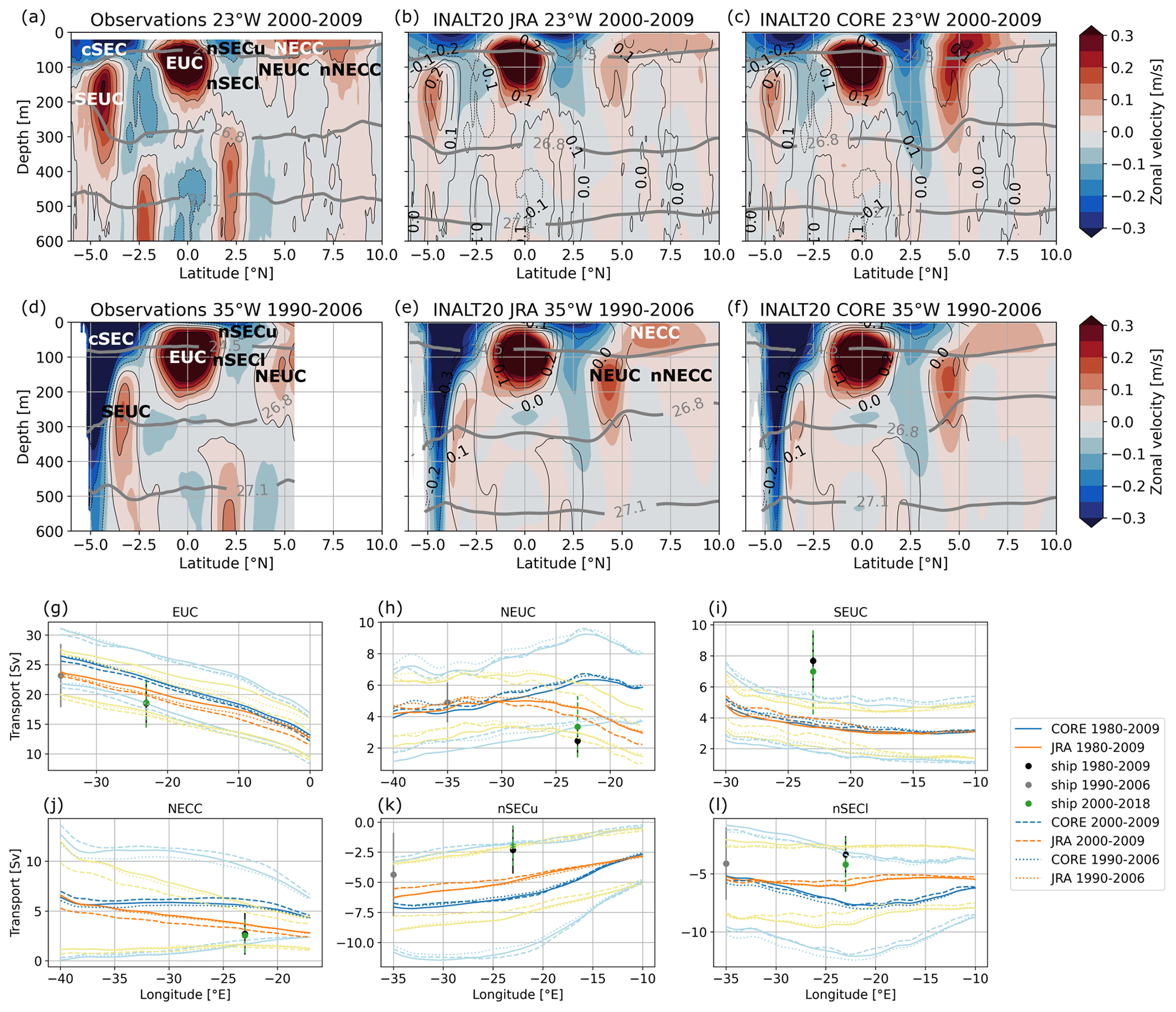
Figure 2 Mean zonal velocity along (a–c) 23° W (2000–2009) and (d–f) 35° W (1990–2006) from (a, d) observations, (b, e) JRA_sim and (c, f) CORE_sim. Eastward velocities are positive (red), and westward velocities are negative (blue). Grey thick contours mark potential density surfaces (kg m⁻³). Thin black contours in panels (a)–(f) mark the observed velocities. (g–l) Temporal mean transport calculated for different periods (solid from 1980–2009; dashed from 2000–2009; dotted from 1990–2006) from the 5 d model output of CORE_sim (blue lines) and JRA_sim (orange lines), as well as ship sections (black dots from 2000–2009; green dots from 2000–2018; grey dots from 1990–2006), using Eq. (2) and the parameters listed in Table 1. The pastel blue and orange lines, as well as the black, green and grey bars, represent 1 standard deviation of model output and ship section in their respective temporal resolution.

To assess how much of the inter-simulation differences in the flow field can be attributed to the wind stress fields and the resulting Sverdrup transport, we use the depth-integrated vorticity equation. Under Sverdrup balance and to leading order, it can be expressed as the balance of the linear advection term $\mathit{\beta }{\mathit{\rho }}_{\mathrm{0}}{\int }_{-H}^{\mathrm{0}}v\mathrm{d}z$ and the wind stress curl, where v is the simulated meridional velocity and H=500 m is the depth of the active ocean layer of interest (Small et al., 2015). Please note, the balance requires an integration depth where the vertical velocity is zero. Given that the isopycnals along 500 m are quite flat in the mean sections at 35 and 23° W we assume that this criterion is approximately fulfilled for long-term means. Differences between the linear advection term and the wind stress curl show where the Sverdrup balance does not hold, for example at the western boundary (Fig. A1). When subtracting the wind stress curl from the linear advection term, the magnitudes in JRA_sim and CORE_sim compare better in the central basin while differences remain in the spatial pattern. The inter-simulation differences in the wind stress curl and the associated Sverdrup balance hence can explain only part of the difference found in the flow field north of the Equator.

The off-equatorial subsurface currents (NEUC and SEUC) are suggested to be partly driven by the pull of upwelling within domes or at the eastern boundary (Furue et al., 2007, 2009; McCreary et al., 2002), and previous observational and model studies found a link between the upwelling regions in the Atlantic and the NEUC (Stramma et al., 2005; Hüttl-Kabus and Böning, 2008; Goes et al., 2013), as well as the SEUC (Doi et al., 2007). We box-averaged the temporal mean (1980–2009) of wind stress curl and Ekman pumping within the Guinea upwelling region (5–10° N, 30–15° W) and found them to be 1.5 times higher in CORE_sim ($\mathrm{1.9}\times {\mathrm{10}}^{-\mathrm{8}}$N m³; 0.8 µm s⁻¹) compared to JRA_sim ($\mathrm{1.2}\times {\mathrm{10}}^{-\mathrm{8}}$N m³; 0.5 µm s⁻¹). The zonally averaged temporal mean (1980–2009) of the NEUC transport west of 25° W is also 1.5 times higher in CORE_sim (6 Sv) compared to JRA_sim (4 Sv). In contrast, the SEUC has a similar mean strength in the two simulations, as do the box-averaged temporal mean (1980–2009) of wind stress curl ($\mathrm{3.7}\times {\mathrm{10}}^{-\mathrm{8}}$N m³) and Ekman pumping (2.5 µm s⁻¹), in a subregion of the Angola Dome region (7.5–4.5° S, 0.5° W–2.5° E) that has been linked to the SEUC by Doi et al. (2007). The comparison of current strength, wind stress curl and Ekman pumping in the upwelling domes between the two simulations suggests that the inter-simulation differences in the NEUC are likely due to differences in the wind stress curl and associated upwelling in the Gulf of Guinea. The good inter-simulation agreement of the SEUC transport fits well to the good agreement of the wind-driven upwelling in the Angola Dome found between the two simulations.

The eastward-flowing NECC has been also shown to be partly connected to the Guinea Dome (Stramma et al., 2005; Hormann et al., 2012; Stramma et al., 2016). Similar to the NEUC, we find that the NECC is on average 1.5 times stronger in CORE_sim (5.4 Sv) than in JRA_sim (3.7 Sv) east of 30° W. Furthermore, the negative wind stress curl anomaly east of 23° W between 3 and 5° N drives eastward Sverdrup flow at 5° N, strengthening the NECC and NEUC in CORE (Fig. 1c). The zonal transport resulting from the meridional Sverdrup transport between 4 and 6° N (U_Ψ; Eq. 11) shows eastward flow in CORE_sim, which is 1 Sv (30° W) to 2.7 Sv (20° W) higher than in JRA_sim. Regarding the entire meridional extent of the NECC (3–10° N), the mean current transport (JRA is 5.2 Sv; CORE is 5.7 Sv) and U_Ψ (JRA is 5.5 Sv; CORE is 5.4 Sv) agree well at 35° W in the two simulations, while they start to diverge further east, with eastward U_Ψ flow in CORE being up to 0.9 Sv (23° W) stronger than in JRA. The anomalous Sverdrup stream function also suggests that CORE drives a strong recirculation between the nSEC and NECC/NEUC, which agrees with the findings of Burmeister et al. (2019) and shows enhanced westward flow along the core position of the nSEC in CORE (Fig. 1c). However, the comparison between the wind stress curl and the linear advection term (Fig. A1) highlights that inter-simulation differences in the wind stress curl and associated Sverdrup transport can only partly explain the inter-simulation differences in the flow field in that region. The surface-flowing nSEC is mainly driven by the equatorial easterlies. The mean zonal wind stress (1980–2009) box-averaged above the SEC region (0–5° N, 35–15° W) is 1.2 times stronger in CORE_sim compared to JRA_sim, as are the zonally averaged current transport for both the nSECu and nSECl.

One of the reasons for the inter-simulation discrepancies might be the coarser spatial resolution of the CORE forcing. Due to its high spatial resolution, the JRA forcing is thought to better resolve fine wind stress curl structures. To get an idea how much the spatial resolution matters, we bin-averaged the wind stress fields of the two simulations to a spatial resolution of 2° × 2° (Fig. A5). Compared to JRA_sim, CORE_sim still shows increased positive wind stress curl along the western boundary, in the central basin along 5° N, within the Guinea Dome region and along northwestern Africa. However, the difference in the Sverdrup stream function between the coarse resolution fields of JRA_sim and CORE_sim (Fig. A5f) does not show any small-scale features visible in the high-resolution fields above the nSEC and NECC/NEUC region, with differences in the Sverdrup stream function of 0.5 to 1.5 Sv east of 30° W (Fig. 1c).

The EUC is mainly driven by the easterly winds along the Equator (Pedlosky, 1987; Wacongne, 1989). However, Arhan et al. (2006) showed that in the absence of the equatorial zonal wind during winter and spring, EUC transport can be remotely forced by the wind stress curl between 2° N and 2° S, connecting it to the western boundary currents. The mean zonal wind stress (1980–2009) in CORE_sim along the Equator is stronger (−0.034 N m⁻², with a standard deviation of ±0.012 N m⁻²), than in JRA_sim (−0.027 N m⁻², with a standard deviation of ±0.011 N m⁻²). The intermodel difference in the mean wind stress can be one reason why the EUC transport is stronger in CORE compared to JRA. Another process impacting the strength of the EUC is the strength of the STCs. The different levels of strength of the trade winds between the forcings may lead to a different level of strength in the poleward Ekman transport, forming the upper branch of the STCs which again can cause a different level of strength in the EUC (Rabe et al., 2008). The strength of the STCs is related to the meridional Ekman, divergence which is quantified as the divergence of the Ekman transport (Eq. 12) between 10° S (JRA_sim −9.4 Sv; CORE_sim -11 Sv) and 10° N (JRA_sim 9.3 Sv; CORE_sim 11.4 Sv). The calculated meridional Ekman divergence for the two simulations (JRA_sim 18.7 Sv; CORE_sim 22.4 Sv) is within the range of estimates derived for different wind products in Tuchen et al. (2019, 20.4±3.1 Sv). We find that the meridional Ekman divergence in CORE_sim is 3.7 Sv larger than in JRA_sim, which can contribute to a stronger mean EUC transport in CORE_sim compared to JRA_sim. Furthermore, at 35° W (23° W), the difference in the mean eastward Sverdrup transport between 2° N and 2° S for the period 1980 to 2009 is 2.2 Sv (0.2 Sv) higher in CORE_sim than in JRA_sim, which might also contribute to a stronger EUC in CORE_sim, especially west of 20° W.

3.2 Seasonal cycle

The seasonal cycle in the tropical Atlantic circulation is dominated by the meridional migration of the ITCZ and concomitant changes in the wind field (e.g. Xie and Carton, 2004). In the following, we investigate how differences in the seasonal cycle of the wind forcings impact the seasonal cycle of the zonal currents. First, we show the main patterns of the seasonal cycle of the wind forcing by fitting the annual harmonic to the zonal wind stress and wind stress curl for the period 1980 to 2009 (Fig. 3). Then, we describe the seasonal cycle of the simulated path following current transport (Eq. 2) for the same period (Fig. 4). This is followed by a model validation, where we focus on the transport of the EUC and NEUC for the period 2000–2018, when we have moored transport observations available, which are calculated within a fixed box for consistency between model and observations (Fig. 5). Finally, we investigate the link of the seasonal cycle between the wind forcing and the velocity field in the two simulations under the aspect of resonant equatorial basin modes (Fig. 6).

The large-scale pattern of the zonal wind stress and wind stress curl amplitudes of the annual harmonic cycle are similar in the two simulations, while CORE_sim produces much higher amplitudes compared to JRA_sim (Fig. 3). Again, the wind stress curl is characterised by fine spatial structures in JRA_sim, which are not present in CORE_sim. Largest differences in zonal wind stress and wind stress curl occur north of the Equator in the eastern basin. The spatial pattern of the phase of the annual harmonic differs between the simulations for zonal wind stress. This leads to phase shifts between the simulations of 0 to 6 months, depending on longitude and latitude. The spatial pattern of the phase of the wind stress curl agrees better between the two simulations. However, between 4° N and 4° S, west of 20° W, the phase is very homogeneous in JRA_sim, while we see a change in phase with longitude of up to 6 months in CORE_sim. The annual harmonic amplitude of zonal wind stress along the Equator is much larger in CORE_sim compared to JRA_sim. Before we investigate how these differences in the wind forcing impact the zonal current variability, we first describe and validate the seasonal cycle of simulated zonal current transport.

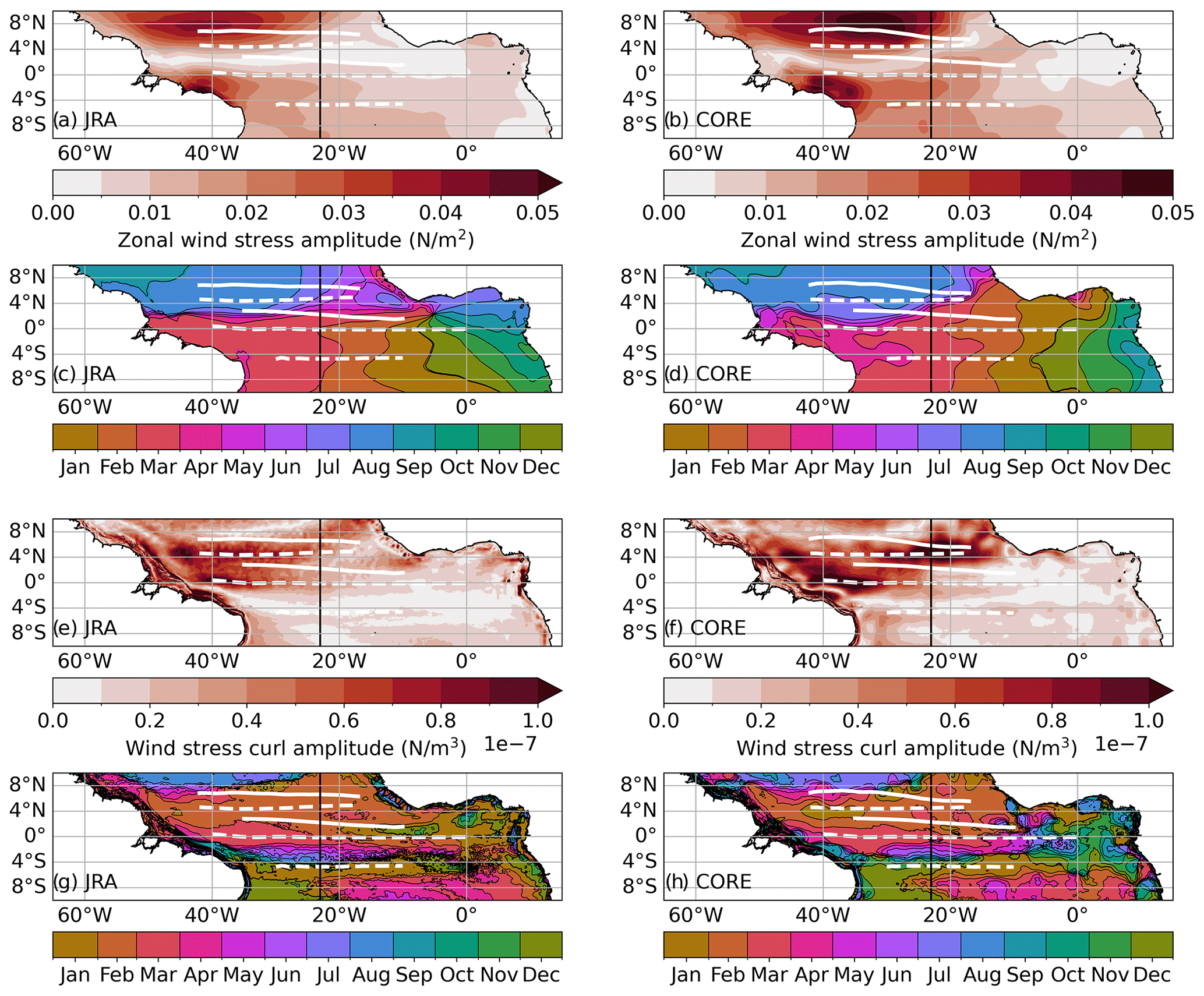
Figure 3 Amplitude (a, b, e, f) and phase (c, d, g, h) of the annual harmonic fitted to the monthly mean climatology of zonal wind stress (a–d) and wind stress curl (e–h) from JRA_sim (left) and CORE_sim (right) for 1980–2009. Zonal white lines mark the mean latitude (Y_CM; Eq. 1) of the simulated surface (solid) and subsurface (dashed) currents for the respective periods. The vertical black lines mark 23° W. Please note that the phase is given as the month of the year when the corresponding amplitude is maximum.

Compared to JRA_sim, CORE_sim exhibits a stronger annual and semi-annual cycle of the zonal current transport, especially at 23° W, except for the SEUC (solid lines in Fig. 4). Aligning with the results for the mean current strength (Fig. 2), the seasonal variability in the SEUC is very similar in the two simulations, and the model tends to underestimate the SEUC strength compared to observations (Fig. 4g). At 23° W, for the EUC and nSECu, the amplitude of the annual cycle in JRA_sim peaks in late boreal spring/early summer, 2 to 3 months earlier than in CORE_sim. For the other currents and for the phase of the semi-annual cycle, the two simulations are in good agreement at 23° W. In general, we find a better agreement between the two simulations regarding the phase and amplitude of the seasonal current transport at 35° W (dashed lines in Fig. 4) than at 23° W.

To get a better understanding of how realistic the model simulates the seasonal cycle of the currents, we compare the seasonal cycle of the simulated currents with moored transport time series available for EUC and NEUC at 23° W only. Note that the reconstructed transport from moored observations is integrated in a fixed box. To compare transport derived from model output and moored observations at 23° W, we calculate the transport for the EUC and the NEUC from model output as the integral of eastward velocity in the respective box (EUC 30–300 m, 1.2° N–1.2° S; NEUC 60–270 m, 4.25–5.25° N). Furthermore, the transport for the seasonal, annual and semi-annual cycles in the following is calculated for a shorter time period covering the time period of observations if possible (see the caption of Fig. 5 for more detail).

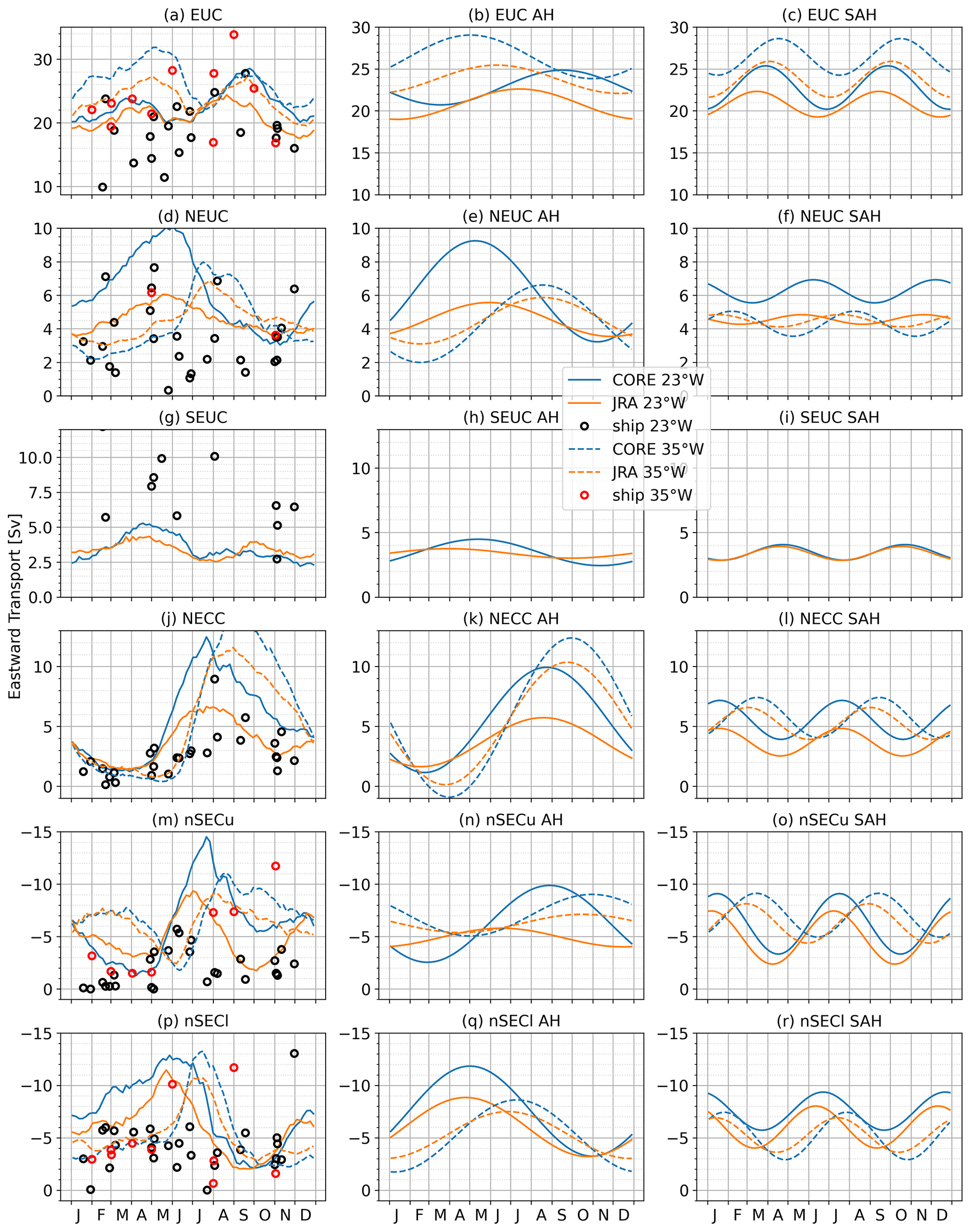
Figure 4 The seasonal cycle (left), annual harmonic (middle) and semi-annual harmonic (right) fitted to the transport time series (Eq. 2) estimated from JRA_sim (orange lines) and CORE_sim (blue lines) at 23° W (solid lines) and 35° W (dashed lines) and averaged over the period 1980 to 2009. Black and red circles in the left column mark the transport estimated from ship sections along 23° W (black) and 35° W (red).

At 23° W, CORE_sim better represents the phase of the annual cycle of the EUC (Fig. 5e–g). We find a 3-month phase shift in the annual cycle in JRA_sim compared to observations. The phase shift in the annual cycle between CORE_sim and the observations is 1 month (Fig. 5f). For the semi-annual harmonic, JRA_sim seems to better represent the amplitude of the observations, while both simulations show a phase shift of about 1 month compared to observations (Fig. 5g). Within the chosen parameters (Table 1), JRA_sim cannot reproduce the EUC intensification in boreal autumn, which seems to be related to the annual cycle peaking in boreal summer. Note that increasing the half-mean width W in Eq. (2) from 2 to 3° results in a 2 Sv increase in the seasonal cycle of EUC transport in boreal autumn (2006–2018), and the fitted annual harmonic is maximum at the end of July (dashed lines in Fig. 5e–g).

The representation of the NEUC transport variability is more realistic in JRA_sim compared to CORE_sim (Fig. 5). JRA_sim better captures the sporadic intraseasonal fluctuations in the NEUC, which is dominating the NEUC variability in the observations (Burmeister et al., 2020). In CORE_sim, the NEUC variability is dominated by a strong seasonal cycle instead (amplitude of 1.8 Sv) even though the spectral analysis of the NEUC in CORE_sim is more energetic on an intraseasonal timescale compared to JRA_sim and observations. Compared to observations, the seasonal cycle of the NEUC in JRA_sim is more realistic but still too strong (JRA_sim 0.6 Sv vs. observations 0.2 Sv). JRA_sim produces a NEUC flow maximum in April to May, which is not visible in the observations, but both the simulated and observed seasonal NEUC cycle show a minimum in boreal autumn. Burmeister et al. (2020) suggested that the NEUC fluctuations might be triggered by Rossby waves which can alter the weak eastward flow of the NEUC. They showed, among others, that small-scale wind stress curl anomalies off the coast of Liberia lead NEUC fluctuations by 1–2 months. Our results suggest that the JRA wind forcing seems to better resolve mechanisms dominating NEUC variability, while CORE_sim seems not to be able to resolve them (Fig. 3e and f). Instead, the annual cycle of the wind stress curl in CORE_sim shows high amplitudes between 4 and 8° N west of 30° W, which might contribute to the strong annual cycle of the NEUC. In CORE_sim, the amplitude of the annual cycle of the wind stress curl averaged in that region (4–8° N, 30–15° W) is twice as strong as in JRA_sim.

The semi-annual and annual zonal flow variability along the Equator is attributed to the resonance period of the gravest basin mode for the second and the fourth baroclinic mode, respectively (Brandt et al., 2016). We perform a baroclinic modal decomposition of the zonal velocity field in the two model simulations to investigate possible resonances and the dynamical response of the ocean to the two wind forcings. We fit the annual and semi-annual harmonic to the first five baroclinic modes. In both simulations, we find high amplitudes of the annual harmonic along the Equator for baroclinic modes four (Fig. 6) and three (Fig. A3). Along the Equator, velocity amplitudes for the annual cycle of baroclinic modes three and four in CORE_sim are up to 2.5 cm s⁻¹ higher than in JRA_sim, with the largest difference occurring between 30 and 20° W for baroclinic mode three (Fig. A3). This agrees with Brandt et al. (2016), who found that the third mode in their model simulation also forced with CORE was enhanced compared to observations. Along the Equator, the phase of the maximum velocity of the annual cycle differs between the two simulations (Fig. 6). Between 0 and 40° W along the Equator (±0.5°), maximum velocities in JRA_sim occur on average 22 d earlier than in CORE_sim, with a standard deviation of 6 d. For the semi-annual cycle, the differences are less distinct (Fig. A2), which is in agreement with the EUC transport time series (Fig. 5). As the phase velocities of the first five baroclinic modes in the two simulations are similar (Table 2), it is likely that the differences are mainly due to the annual cycle of the wind forcing.

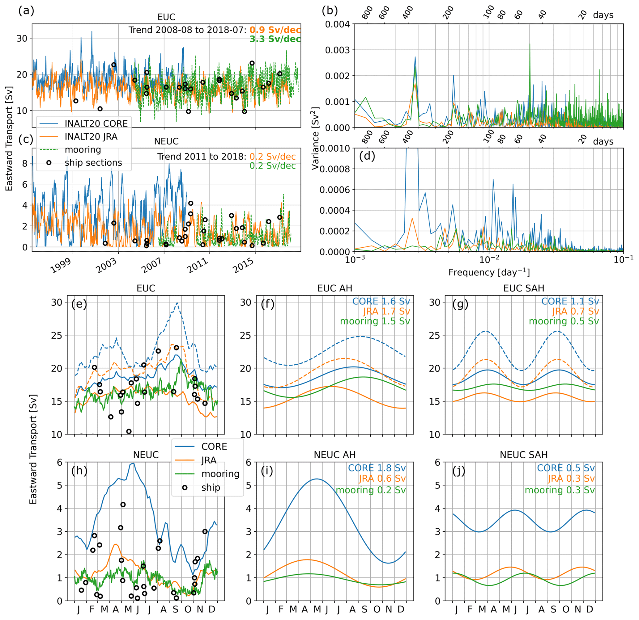
Figure 5 (a, c) Fixed box (EUC is 30–300 m; 1.2° N–1.2° S; NEUC 60–270 m, 4.25–5.25° N) eastward transport time series (solid lines) and (b, d) power spectra of the EUC (a, b) and NEUC (c, d) calculated from CORE_sim (EUC in June 1996–December 2009; NEUC in November 2001–December 2009; blue lines), JRA_sim (EUC in June 2005–December 2018; NEUC in November 2010–December 2018; orange lines), moored observations (EUC in June 2005–December 2018; NEUC in November 2010–December 2018; green lines) and ship sections (black circles) at 23° W. (e, h) Seasonal cycle, (f, i) annual harmonic and (g, j) semi-annual harmonic of (e–g) EUC and (h–j) NEUC. Numbers in panels (f), (g), (i) and (j) represent the amplitude of the fitted harmonic cycle for each time series, respectively. The dashed lines in panels (e)–(g) show the results derived from eastward transport for the EUC calculated using Eq. (2), with a half-mean width W of 3° (CORE_sim in June 1996–December 2009, blue dashes lines; JRA_sim in June 2005–December 2018, orange dashes lines).

Along 5° N within the NEUC region, the amplitude of the annual cycle of the fourth baroclinic mode is slightly higher in CORE_sim and extends further east compared to JRA_sim (Fig. 6). Largest differences in annual cycle amplitudes exist for the first two baroclinic modes just north of the NEUC mean position and south of the nSEC mean position (Fig. A3). This might be one factor explaining why we find a strong annual cycle for the NEUC in CORE_sim and a weak annual cycle in JRA_sim.

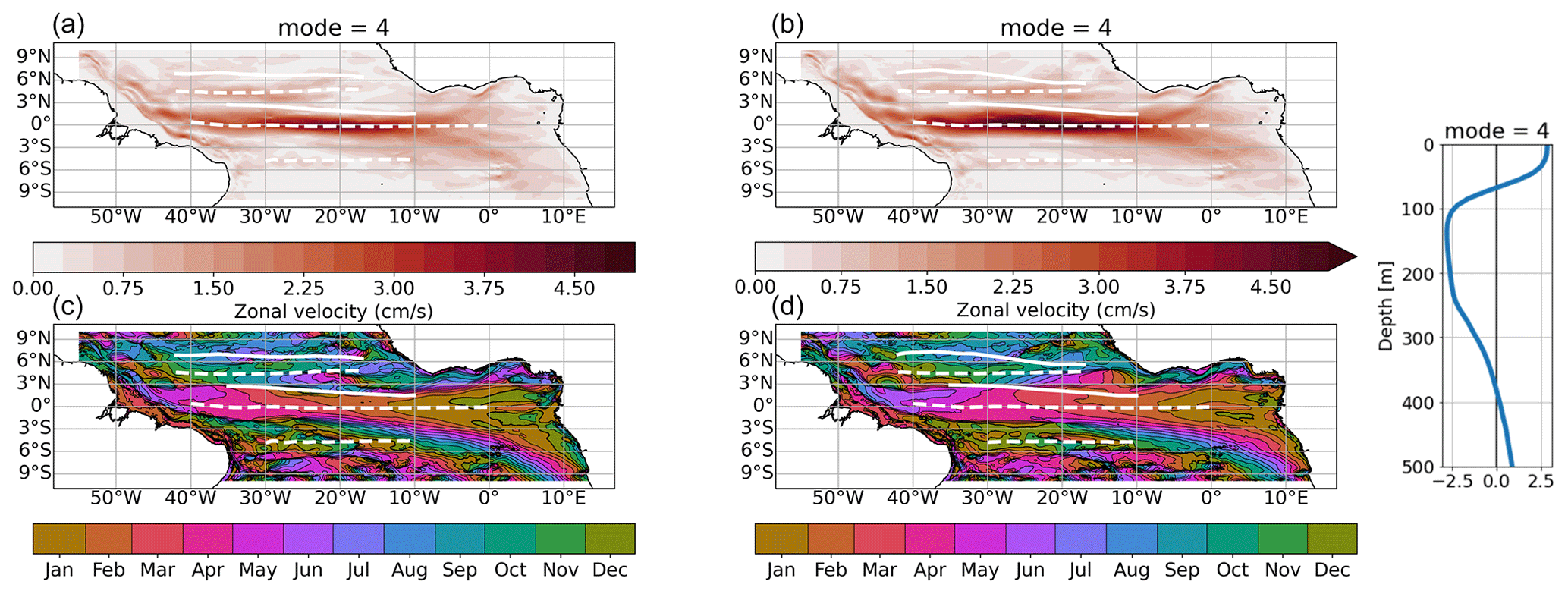
Figure 6 Amplitude (a, b) and phase (c, d) of the fourth baroclinic mode with annual cycle of the zonal velocity from JRA_sim (a, c, 2000–2018) and CORE_sim (b, d, 1991–2009). To derive the 3D zonal velocity field associated with the specific baroclinic mode, the amplitudes must be multiplied by the corresponding vertical structure function shown on the right. The phase is given in month of the year when maximum eastward velocity occurs at the surface. Zonal white lines mark the mean latitude (Y_CM; Eq. 1) of the simulated surface (solid) and subsurface (dashed) currents for the respective periods.

Parts of the NEUC and SEUC are thought to be driven by mesoscale eddies or vortices (e.g. Jochum and Malanotte-Rizzoli, 2004; Assene et al., 2020). Among others, the Eliassen–Palm flux of tropical instability waves (TIWs) is thought to maintain the eastward subsurface currents against dissipation (Jochum and Malanotte-Rizzoli, 2004). Assene et al. (2020) described how westward-propagating mesoscale vortices (e.g. TIWs) east of 20° W can create high potential vorticity gradients in the mean fields which are associated with the NEUC and SEUC. TIWs are mainly generated by shear instabilities between the nSEC and NECC (Philander, 1978; Athie and Marin, 2008) and between the EUC and the nSEC, as well as baroclinic instability within the nSEC and cSEC (Weisberg and Weingartner, 1988; Jochum et al., 2004; von Schuckmann et al., 2008). Inter-simulation differences in the strength of the EUC, nSEC and NECC might generate differences in TIW activity. How the mesoscale dynamics impact the seasonal cycle of the off-equatorial subsurface currents is not clear and beyond the scope of the paper. However, comparing the seasonal cycle of TIW activity between the simulations might give additional insights into why we find different seasonal cycles for the NEUC but not for the SEUC in the two simulations. In general, we find a higher TIW activity in CORE_sim compared to JRA_sim (Fig. 7). Within the NEUC region, we find that the seasonal cycle of the TIW activity in CORE_sim is dominated by an annual cycle, and the seasonal maximum is nearly twice as high as in JRA_sim (Fig. 7). The seasonal cycle of the TIW activity in JRA_sim peaks in August and January and does not reveal a clear annual cycle. The seasonal cycle of TIW activity in the SEUC region agrees well between the two simulations and peaks in March and August. The differences in the seasonal cycle of mesoscale activity within the NEUC region between the two simulations might impact NEUC variability and hence contribute to the inter-simulation discrepancies found.

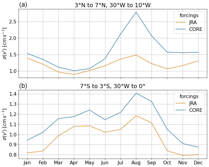
Figure 7 Monthly standard deviation of band-pass-filtered meridional velocity at 160 m depth from JRA_sim (orange line) and CORE_sim (blue line) temporally averaged over the period 1980 to 2009 and spatially averaged within the NEUC (top) and SEUC regions (bottom).

3.3 Long-term variability and trends

In this section, we investigate the interannual and longer-term variability, as well as linear trends of the wind field and current transport in the simulations. Although longer-term variability and trends in the wind forcings are very uncertain, the wind field is expected to change under global warming. It is important to understand how longer-term changes and trends are related to changes in zonal currents. We start by briefly summarising the long-term variability and trends found by previous studies in the moored transport reconstructions of the EUC (Brandt et al., 2021) and NEUC (Burmeister et al., 2020) and briefly check if we can reproduce the results in JRA_sim for an initial validation. This is not possible for CORE_sim, as it does not cover the time period of observations. Linear trends are fitted to the time series within the given period from which the annual and semi-annual harmonic were removed. Then we calculate the autocorrelation to find the degrees of freedom using the e-folding timescale. Finally, we test the significance of the trend using a two-sided t test.

The 8-year moored transport time series of the NEUC is dominated by sporadic intraseasonal variability and does not reveal any longer-term variability or a linear trend between 2010 and 2018 (Fig. 5c, d; Burmeister et al., 2020). JRA_sim realistically represents the result of the observations, except for a small peak in the power spectra for the annual cycle, which is not present in observations.

Brandt et al. (2021) observed that the EUC transport increased significantly by 3.3 Sv/dec at 23° W between 2008 to 2018 (see also Fig. 5a). In JRA_sim, we find a significant but weaker increase in the EUC transport (0.9 Sv/dec) for the same period (Fig. 5a). Brandt et al. (2021) found that an intensification of trade winds in the western tropical North Atlantic, and the concurrent strengthening of the STCs and enhanced Ekman divergence (1.1–2.0 Sv/dec depending on the wind product) can explain part of the observed EUC intensification. They suggested that the increase in the northeasterly trade winds might be associated with the Atlantic multidecadal variability (AMV; Delworth and Greatbatch, 2000), which switched from a warm phase in 2000s to a recent cold phase (Frajka-Williams et al., 2017). In JRA_sim, we find the Ekman divergence increases significantly by 1.4 Sv/dec between 2008 and 2018, which agrees well with the results of Brandt et al. (2021). However, the increase in the EUC during this period in JRA_sim is weaker.

The advantage of this study is that both model simulations go back to 1958, which enables us to compare the interannual to decadal variability in the wind forcings and the simulated zonal wind-driven current field. While the observational studies are not able to clearly identify if the linear trend found over the 10 years of observations is part of a longer-term variability or not, the longer time series from the simulations allow us to do so. Nevertheless, results especially with respect to decadal and longer variability must be regarded with great care, as the forcing products are based on observations which span different time periods and fluctuate in their spatial coverage. Hence, the decadal to longer-term variability in the simulations might not represent reality, especially in the earlier periods.

In the following, we removed the monthly mean seasonal cycle from 1980 to 2009 and averaged the simulated time series annually, which reveals the interannual to decadal variability. Please note that in the following we use the path-following algorithm (Eq. 2) for the current transport of the individual zonal currents.

3.3.1 The wind field

The annual mean zonal wind stress anomalies in CORE_sim are stronger than those obtained for JRA_sim, especially before 1970 (Fig. 8). For this early period, limited availability of observations on which the forcing products are based might be one reason for the large inter-simulation discrepancies. While similarities between the two forcings exist in the western basin, differences increase toward the east of the basin. The largest differences between the two forcing products occur north of the Equator before 1990.

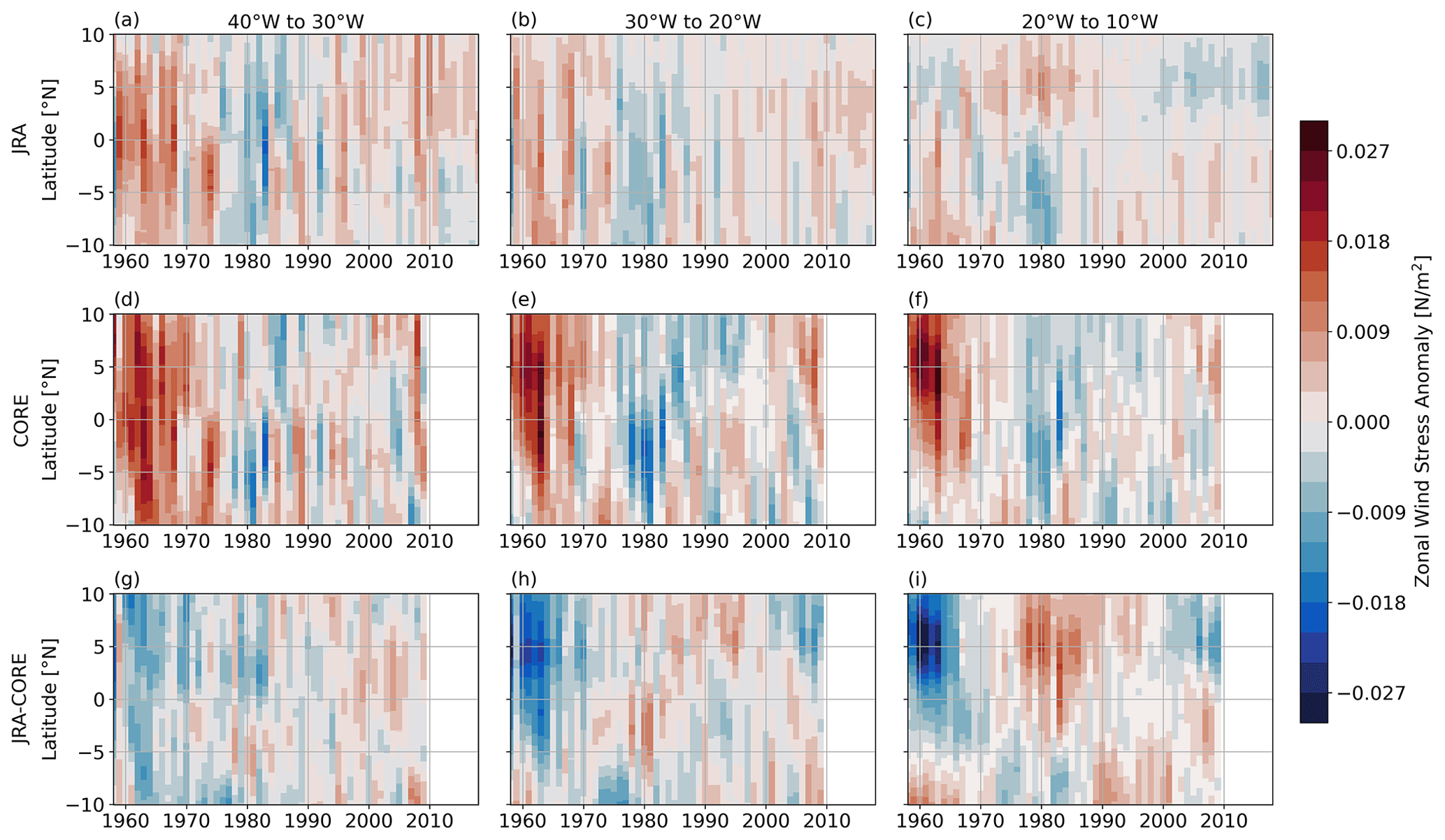
Figure 8 Hovmöller diagram of annual mean zonal wind stress anomalies zonally averaged between 40 and 30° W (a, d, g), 30 and 20° W (b, e, h) and 20 and 10° W (c, f, i) for JRA_sim (a–c), CORE_sim (d–f) and the difference in JRA_sim–CORE_sim (g–i). The anomalies are calculated by removing the seasonal cycle (1980–2009) from the monthly mean output before temporally averaging to annual resolution.

To get a first impression of how these spatial dissimilarities of the wind stress anomalies impact the zonal currents, we calculate the Sverdrup stream function (Eq. 10), using the annual mean wind stress curl anomalies, which we then average for different time periods (Fig. 9b–f). As a reference, we calculate the Sverdrup stream function from the mean wind stress curl field from 1980 to 2009 (Fig. 9a). For comparison with the model flow field, we also calculate the anomalies of the stream function of the depth-integrated velocity field of the upper 500 m (not shown), which compares well with the anomalous Sverdrup stream function, indicating the importance of the Sverdrup stream function for interdecadal changes in the flow field. The spatial differences in the wind field anomalies result in distinct anomalous Sverdrup transport between the simulations, often with the opposite sign for the shown periods. In the following, we present and discuss the longer-term variability and its connection to the wind field for each current separately. Therefore, we calculate the annual mean anomalous volume transport for each current (Fig. 10). Additionally, we calculate the difference in the annual mean anomalous Sverdrup stream function between the approximate latitudinal boundaries (Eq. 11) of the currents at given longitudes (Fig. 11), assuming that the difference represents the zonal transport at that longitude (positive westward; negative eastward).

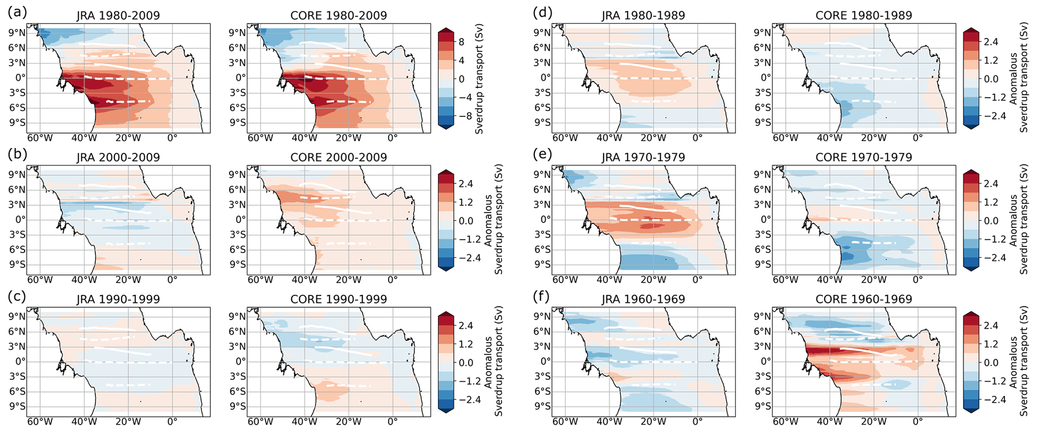
Figure 9 Sverdrup stream function calculated from (a) the 1980–2009 mean wind stress curl field. (b–f) Annual mean wind stress curl anomalies averaged for the periods (b) 2000–2009, (c) 1990–1999, (d) 1980–1989, (e) 1970–1979 and (f) 1960–1969. In panels (b)–(f), we first calculate the Sverdrup stream function from the annual mean wind stress curl anomalies and average then over the respective periods. A negative stream function presents an anticlockwise rotation; this means that a zero contour of the stream function with negative values in the south (north) marks maximum westward (eastward) velocities. Zonal white lines mark the mean latitude (Y_CM; Eq. 1) of the simulated surface (solid) and subsurface (dashed) currents for the respective periods.

3.3.2 EUC

Before 1980, EUC transport is generally increasing in the two simulations (Fig. 10a–b). However, while the lowest EUC transport anomalies (up to −6 Sv) across the entire time series occur in CORE_sim before the mid-1970s, transport anomalies in JRA_sim are still slightly positive during that period. Between 1980 and 2009, the EUC transport decreases in the two simulations (JRA_sim −1.0 Sv/dec; CORE_sim −0.4 Sv/dec), which is significant at a 95 % confidence level (Table 3). This is opposite to the increase in the EUC in the most recent decade (2008–2018) in observations and in JRA_sim (Figs. 5 and 10a). Note that even though we find a strengthening of the EUC in JRA_sim in the last 10 model years, with respect to the 1980–2009 climatology, it is still anomalously weak.

Simultaneous to the EUC strengthening before the 1980s, easterly winds along the Equator are intensifying in the two simulations, with stronger westerly wind anomalies before 1970 in CORE_sim compared to JRA_sim (Fig. 8). This is accompanied by a positive trend in the Ekman divergence of 3.6 Sv/dec in JRA_sim and 3.9 Sv/dec in CORE_sim between 1960 and 1980. Likewise, the easterlies along the Equator tend to decrease after the mid-1980s, and we find a negative trend as well in the Ekman divergence between 1980 and 2009 of −1.5 Sv/dec in JRA_sim and of −0.9 Sv/dec in CORE_sim. Consequently, the EUC transport weakens during this period. Still, interannual anomalies of EUC transport differ between CORE_sim and JRA_sim, which we link to the anomalous Sverdrup transport between 2° N and 2° S (Arhan et al., 2006). Before 1970, when westerly wind anomalies occur along the Equator in the two simulations, we find anomalous westward Sverdrup transport in CORE_sim (Fig. 11), which is associated with a weakening of the EUC (Kessler et al., 2003; Arhan et al., 2006; Brandt et al., 2014). In contrast, the eastward Sverdrup transport anomalies in JRA_sim along the Equator result in positive EUC anomalies before the mid-1970s. In the second period of anomalously weak easterlies along the Equator from the early 1990s onward, the anomalous Sverdrup transport in CORE_sim switches from eastward before 2000 to westward afterwards, which impacts the EUC transport accordingly. In JRA_sim, the signal in the anomalous Sverdrup transport along the Equator is less clear. However, after 2010, the Ekman divergence acts to strengthen the EUC again, while the easterly winds along the Equator stay anomalously weak. The anomalous Sverdrup transport tends to be negative along the Equator before the mid-2010s, which might counteract the EUC strengthening by the anomalous Ekman divergence.

Brandt et al. (2021) showed that the recent EUC strengthening is mainly related to trade wind changes in the western tropical North Atlantic (5–10° N, 60–40° W), which result in the observed increased Ekman divergence in the tropical Atlantic. In agreement with Brandt et al. (2021), we find a switch from weaker northeasterly winds to stronger northeasterly winds in the western North Atlantic in JRA_sim from 2010 onwards. Due to its effect on the Northern Hemisphere trade winds, Brandt et al. (2021) suggested a link between EUC transport variability and the AMV. The AMV transitioned from a cold to a warm phase from 1970 to 2010 and from a warm to a cold phase before 1970 and after 2010. The northeasterly wind is weakest during a warm phase of the AMV. In general, our results support the idea that the decadal variability in the EUC is connected to the AMV through anomalous Ekman divergence which acts to strengthen (weaken) the EUC during a cold (warm) phase of the AMV.

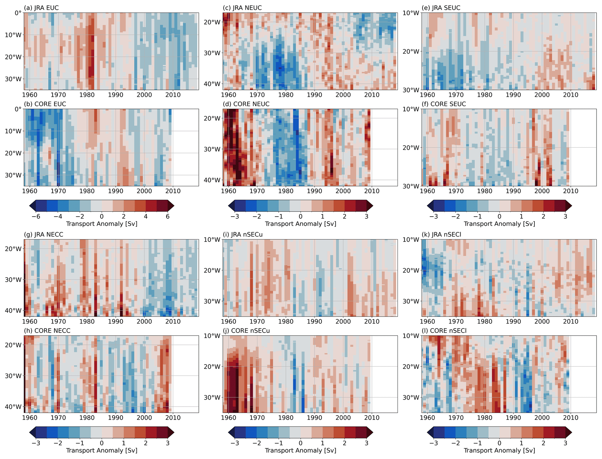
Figure 10 Hovmöller diagram of annual mean transport anomaly (Sv) for (a, b) EUC (eastward current), (c, d) NEUC (eastward current), (e, f) SEUC (eastward current), (g, h) NECC (eastward current), (i, j) nSECu (westward current) and (k, l) nSECl (westward current). The anomalies are calculated by removing the seasonal cycle (1980–2009) from the monthly mean output before temporally averaging to annual resolution.

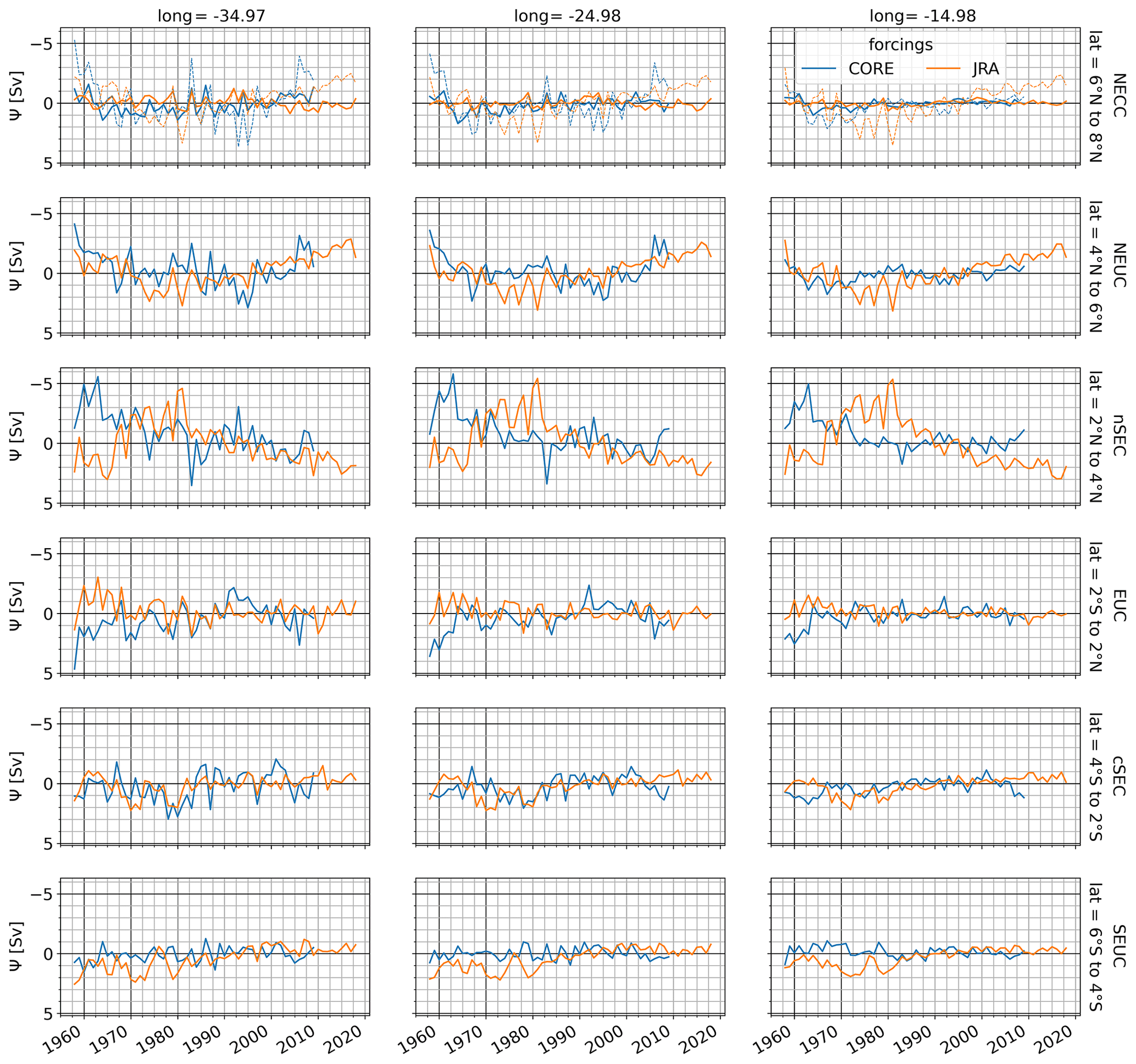
Figure 11 Difference in anomalous Sverdrup stream function Ψ with respect to 1980–2009 climatology calculated for different latitude bands centred above zonal current (rows; southern minus northern Ψ value) for given longitudes (columns) for JRA_sim (orange) and CORE_sim (blue). Dashed lines in the NECC row show the difference in Ψ between 4 and 8° N as the NECC overlaps with the NEUC core position. Note that the y axis is reversed, as negative values indicate eastward flow anomalies.

3.3.3 NEUC

West of 30° W, NEUC transport in the two simulations decreases (switch from positive to negative anomalies) before 1980 and increases afterwards (Fig. 10c–d). At 35° W, we find a significant trend of 0.6 Sv/dec in JRA_sim and 0.8 Sv/dec in CORE_sim between 1980 and 2009 (Table 3). While this signal is zonally coherent in CORE_sim, we find significant negative trends in current transport east of ∼30° W in JRA_sim. In the zonally averaged transport, we cannot find a significant trend in JRA_sim, while the NEUC transport is increasing by 0.8 Sv/dec in CORE_sim.

In JRA_sim anomalies of zonal winds north of the Equator are also not zonally coherent (Fig. 8). West of 20° W, the easterlies north of the Equator are strengthening before 1980, while they are weakening after 1980. In contrast, east of 20° W, the anomalies are reversed. Between 4 and 6° N, the anomalous Sverdrup stream function drives eastward flow when the NEUC west of 30° W is anomalously strong and westward flow when the western NEUC is anomalously weak (Fig. 11). The mean NEUC position west of 30° W is located along zero contours of the anomalous Sverdrup stream function for all decades, except for the 1990s (Fig. 9). East of 30° W, the position of the NEUC is displaced northward of the zero-crossings, which might explain why the NEUC anomalies are not zonally coherent in JRA_sim. In CORE_sim, the NEUC anomalies are significantly correlated (R=0.75), with a strengthening/weakening of zonal easterly winds just north of the Equator (2–8° N, 35–15° W) between 1960 and 2009 (Fig. 12a). This is mainly associated with a switch of positive to negative zonal wind stress anomalies before the 1980s. The correlation decreases for the period 1980 to 2009 (R=0.4).

Goes et al. (2013) suggested a link between the upwelling of the Guinea Dome region and the NEUC on interannual timescales. For the period 1960 to 2009, we find a significant correlation (JRA_sim R=0.50; CORE_sim R=0.47) between the box-averaged wind stress curl (5–10° N, 35–15° W) and the NEUC transport in the two simulations. When repeating the correlation for the period 1980 to 2009, it is still significant but decreases to R=0.39 in JRA_sim, while the correlation becomes non-significant in CORE_sim. In contrast to Goes et al. (2013), the results in JRA_sim suggest a link between the NEUC and the upwelling within the Guinea Dome on interdecadal timescales. In CORE_sim, this link is less clear.

Tuchen et al. (2022b) recently reported decadal variability in TIW activity. As part of the NEUC is eddy-driven (e.g. Jochum and Malanotte-Rizzoli, 2004; Assene et al., 2020), this might lead to long-term changes in the NEUC transport. However, we could not find a clear connection between long-term changes in TIW activity and NEUC transport (Fig. A4).

3.3.4 SEUC

Both model simulations show a significant increase in SEUC transport (JRA_sim 0.4 Sv/dec, CORE_sim 0.3 Sv/dec) between 1980–2009 (Table 3). Anomalies of the long-term variability in the SEUC also tend to be zonally coherent in CORE_sim, while they can be of opposite sign east and west of about 20° W in JRA_sim (Fig. 10e–f). In both simulations, the highest anomalies occur west of 20° W. In JRA_sim, the SEUC west of 20° W shifts from a negative phase before the mid-1990s to a positive phase afterwards. Likewise, the anomalous Sverdrup stream function acts to weaken (strengthen) the eastward flow of the SEUC before (after) the 1990s (Fig. 11). East of 20° W the SEUC in JRA_sim varies by about 1–2 Sv on interannual to decadal timescales.

In CORE_sim, the SEUC seems to covary with the NEUC on decadal timescales, and we find anomalous negative (positive) wind stress curl averaged in a box south of the Equator (10–0° S, 35–15° W) before the 1970s and after 1990s (between 1970 and 1990). The zonal flow associated with the anomalous Sverdrup stream function between 4 and 6° S shows no clear link to the SEUC transport variability on decadal timescales but might explain some of the interannual variability (Fig. 11). The SEUC position in CORE seems to coincide with the maximum Sverdrup stream function, which indicates a meridional exchange with its westward-flanking current bands of the cSEC (Fig. 9). Previous studies showed that the SEUC is mainly fed through recirculation with the ocean interior (Hüttl-Kabus and Böning, 2008; Fischer et al., 2008) and mesoscale eddy fluxes or mesoscale vortices are suggested to be one of the drivers of the SEUC (Jochum and Malanotte-Rizzoli, 2004; Assene et al., 2020). As for the NEUC, however, we could not find a clear connection between long-term changes in TIW activity and SEUC transport (Fig. A4).

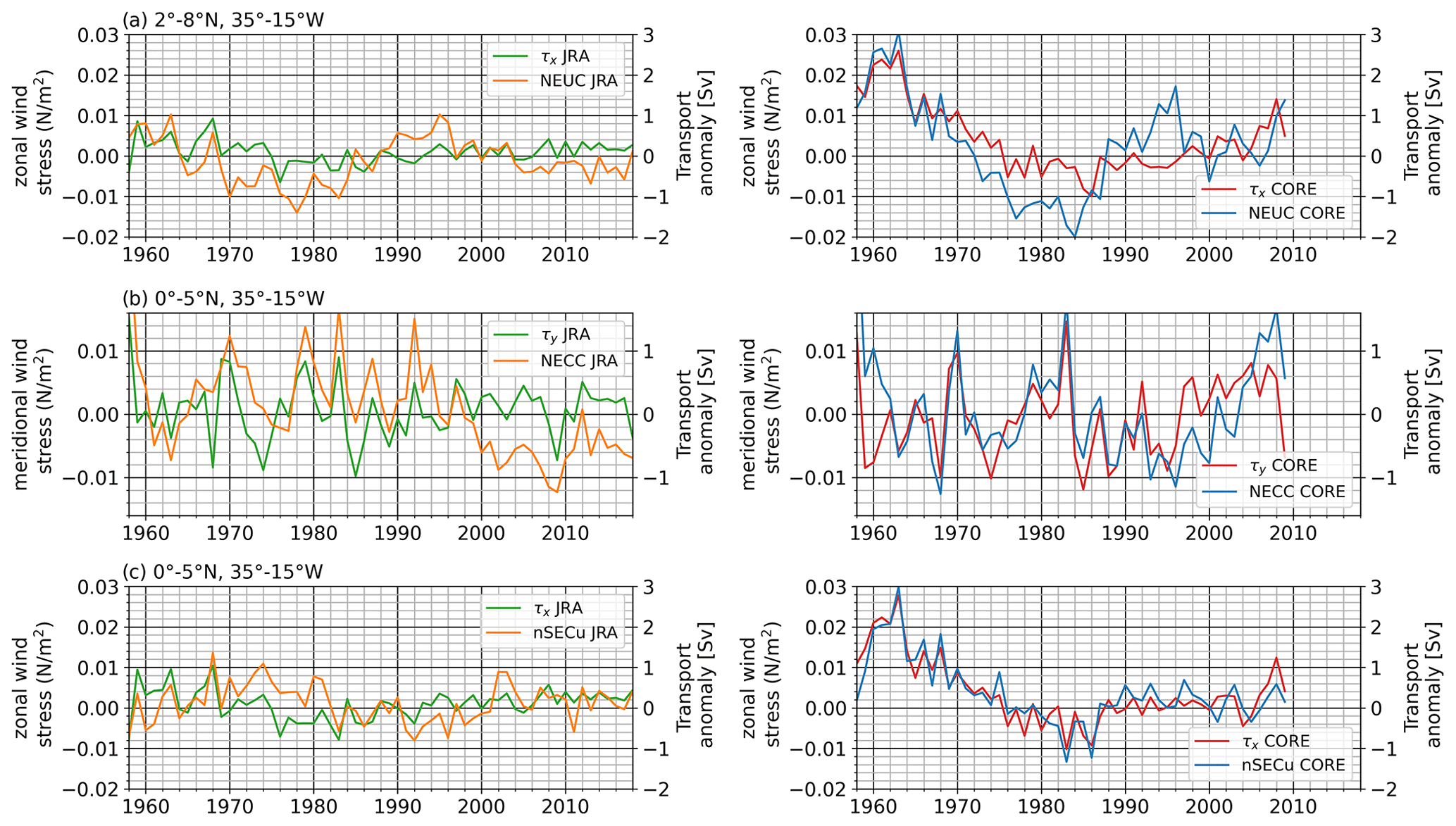
Figure 12 (a) Annual mean zonal wind stress anomalies averaged between 2 and 8° N, 35 and 15° W (green and red lines) and zonally averaged annual mean NEUC transport anomalies (orange and blue lines) for JRA_sim (left) and CORE_sim (right). (b) Annual mean meridional wind stress anomalies averaged between 0 and 5° N, 35 and 15° W (green and red lines) and zonally averaged annual mean NECC transport anomalies (orange and blue lines) for JRA_sim (left) and CORE_sim (right). (c) Annual mean zonal wind stress anomalies averaged between 0 and 5° N, 35 and 15° W (green and red lines) and zonally averaged annual mean nSECu transport anomalies (orange and blue lines) for JRA_sim (left) and CORE_sim (right).

3.3.5 NECC

NECC transport anomalies tend to be zonally coherent in the two simulations (Fig. 10g–h); however, after the mid-1980s, the anomalies are of a different sign in JRA_sim and CORE_sim. We find a decrease of −0.6 Sv/dec in the NECC transport in JRA_sim and an increase of 0.2 Sv/dec in CORE_sim between 1980 to 2009 (Table 3). The NECC anomalies after 1990 are associated with an anomalous Sverdrup stream function of an opposite sign in the NECC region between JRA_sim and CORE_sim (Figs. 9b, c and 11). In CORE_sim, the zonal flow associated with the anomalous Sverdrup stream function between 4 and 8° N seem to better represent the long-term variability in the NECC, while in JRA_sim the anomalous Sverdrup stream function between 6 and 8° N seems to dominate flow variability.

Goes et al. (2013) and Hormann et al. (2012) suggested a link between the NECC variability and the Atlantic meridional mode, one of the dominant modes of tropical Atlantic variability, which is acting on interannual to decadal timescales. The Atlantic meridional mode is characterised by a cross-equatorial sea surface temperature (SST) gradient and anomalous meridional winds blowing from the colder to the warmer hemisphere. It is mainly governed by the wind–evaporation–SST feedback (Carton et al., 1996; Chang et al., 1997). Goes et al. (2013) found a positive correlation between the NECC transport and the meridional wind stress anomalies averaged in the box 0–5° N, 35–15° W just south of the NECC. We find a similar relationship on interannual timescales in the two simulations (Fig. 12b), despite the distinct inter-simulation discrepancies of the NECC on decadal timescales, especially after 2000.

3.3.6 nSEC (upper and lower)

In CORE_sim, the anomalies of the westward-flowing nSECu on interannual to decadal timescales (Fig. 10i–j) are concurrent with anomalous easterlies just north of the Equator (Fig. 8d–f). The nSECu and the easterlies are weaker before the mid-1970s; then, they are stronger until the late 1980s. After 1990, they show weak positive anomalies (weakening) until the 2000s and then covary on an interannual timescale at least between 30–20° W. The correlation coefficient between annual anomalies of zonally averaged nSECu transport and box-averaged zonal wind stress (0–5° N, 35–15° W) is 0.90 at lag 0 in CORE_sim (Fig. 12c). This is not the case in JRA_sim, where the correlation coefficient is 0.35 at lag 0. It seems that the zonal wind stress anomalies (Fig. 8a–c) in JRA_sim lead the nSECu transport anomalies by 5–10 years. Indeed, we find maximum correlation (R=0.45) between annual anomalies of zonally averaged nSECu transport and box-averaged zonal wind stress (0–5° N, 35–15° W), with the wind stress leading 7 years. Still, the correlation between nSECu transport and zonal wind stress is weak compared to CORE.

For the lower part of the nSEC (Fig. 10k–l), the two simulations tend to be in better agreement regarding the long-term variability with stronger nSECl flow before 1970 and during the late 1980s to late 1990s and weaker flow between 1970–late 1980s and after the late 1990s. However, in CORE_sim, anomalies are stronger and seem to propagate from the eastern to the western basin, while this is less clear in JRA_sim. The anomalies of the nSECu and nSECl seem to be largely in phase in JRA_sim, while they tend to vary out of phase in CORE_sim. Interestingly, in JRA_sim after 1980 between 30 and 20° W, the nSEC and the NECC are the two strengthening or weakening at the same time, while this link is less clear in JRA_sim before the 1980s and in CORE_sim for the entire period.

For the zonally averaged nSECu (surface), JRA_sim simulates no significant trend, while CORE_sim shows a significant decrease of 0.2 Sv/dec between 1980 and 2009. For the same period, the zonally averaged nSECl (subsurface) in JRA_sim weakens by 0.1 Sv/dec, while transport strengthened by −0.2 Sv/dec in CORE_sim (Table 3). Looking at trends of the two currents at selected longitudes reveals that they are not zonally coherent in the two simulations. For example, both simulations show a nSECl strengthening of 0.2 Sv at 15° W between 1980 and 2009, while at 35° W the nSECl trend is negative and significant in JRA_sim and negative but not significant in CORE_sim.

Table 3 Linear trends per decade of transport of the currents from 1980 to 2009. Significant trends are shown in bold.

4 Summary and conclusion

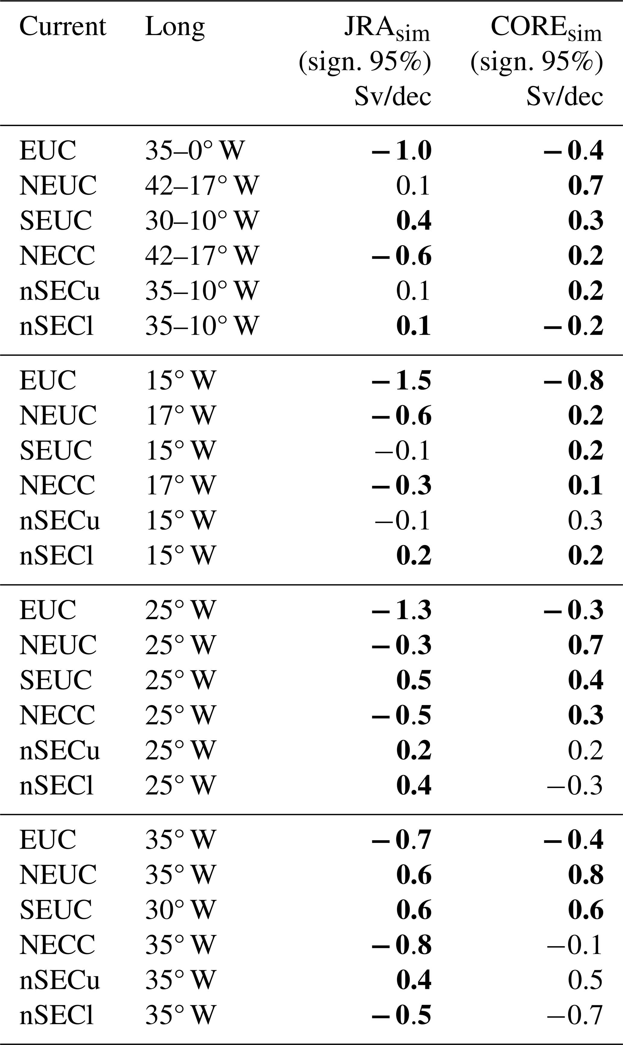
In this study, we investigate the effect of different wind forcings on the representation of zonal current strength and variability in the tropical Atlantic in a general ocean circulation model. The first forcing product is the CORE v2 dataset covering the period 1948 to 2009 (Griffies et al., 2009). It has a horizontal resolution of 2° × 2° and temporal resolution of 6 h. The second forcing product is the JRA55-do surface dataset (Tsujino et al., 2018). This dataset stands out due to its high horizontal (55 km) and temporal resolution (3 h), which covers the entire observational period (1958 to 2018). Where possible, we compare the results to ship sections and moored transport reconstructions along 23 and 35° W (Brandt et al., 2021; Burmeister et al., 2020; Tuchen et al., 2022a).

The wind stress field of the CORE forcing is generally stronger than that of the JRA forcing on all timescales (Figs. 1, 3, 8), which is also reflected in the current transport, except for the SEUC (Figs. 2, 4, 5 and 10). In the mean fields between 1980 and 2009, JRA_sim seems to better represent the EUC, NEUC, NECC and nSECl (Fig. 2). Depending on the individual currents, the two simulations agree better in the western (NEUC, NECC and nSECl) or eastern basin (EUC and nSECu). The SEUC transport agrees well between the two simulations, which both underestimate the SEUC strength compared to observations. We find stronger positive wind stress curl in CORE_sim at the western boundary, as well as north of the Equator in the central basin along 5° N in the Guinea Dome region and along the coast of northwestern Africa (Fig. 1). South of the Equator, away from the western boundary, the mean wind stress curl fields agree well. We find that part of the inter-simulation discrepancies can be explained by the coarser spatial resolution of the CORE forcing, especially east of 30° W, north of the Equator (Figs. 1 and A5). We also find higher wind-driven upwelling in the Guinea Dome in CORE_sim, which can contribute to the higher NEUC transport compared to JRA_sim (Stramma et al., 2005; Hüttl-Kabus and Böning, 2008; Goes et al., 2013). Stronger easterly winds along the Equator can contribute to higher transport of the nSEC and EUC (Wacongne, 1989), which might be one reason for the higher mean current transport in CORE_sim compared to JRA_sim. Additionally, we find higher divergence of the meridional Ekman transport between 10° N and 10° S and higher zonal transport resulting from the meridional Sverdrup transport between 2° N and 2° S in CORE_sim compared to JRA_sim, which again can contribute to inter-simulation differences in the EUC transport (Brandt et al., 2021; Arhan et al., 2006).

CORE_sim generally features a stronger seasonal cycle of the zonal wind stress and wind stress curl (Fig. 3), resulting in stronger seasonal cycle in current transport at 35 and 23° W, except for the SEUC (Fig. 4). The two simulations agree better in amplitude and phase of the zonal wind stress and wind stress curl (Fig. 3), as well as current transport in the western basin than in the eastern basin (Fig. 4). To investigate the dynamical response of the zonal current field to the seasonal wind forcing, we perform a baroclinic mode decomposition (Figs. 6 and A3). The phase speed of the first five baroclinic modes agree well between the two simulations (Table 2), which suggests that the differences in the seasonal cycle of current transport can be mainly attributed to differences in the wind forcing. We find a 2–3 month phase shift in the annual harmonic of EUC transport between the two simulations, with CORE_sim better representing the annual cycle found in observations. JRA_sim realistically captures the sporadic seasonal fluctuations which dominate the NEUC transport variability in observations, while the NEUC in CORE_sim is unrealistically energetic on all timescales and is dominated by an overly strong seasonal cycle (Fig. 5). In contrast, the seasonal cycle of the SEUC transport is in good agreement between the two simulations. Differences in the annual cycle of the first two baroclinic modes between the two simulations may contribute to the discrepancies in the seasonal NEUC transport between CORE_sim and JRA_sim (Fig. A3). We also find different (similar) simulated seasonal TIW activity within the NEUC (SEUC) region between the two simulations (Fig. 7). As the NEUC and SEUC are thought to be partly eddy-driven (e.g. Jochum and Malanotte-Rizzoli, 2004; Assene et al., 2020), this might be another reason for the discrepancies found in the simulated seasonal current transport. However, further analysis is needed to confirm this, which is beyond the scope of this paper.

On interannual to decadal timescales, JRA_sim and CORE_sim show opposite signs of annual mean zonal wind stress anomalies east of 20° W and north of the Equator (Fig. 8g–i). The difference in the spatial pattern of wind field anomalies results in different anomalous Sverdrup flow (Figs. 9 and 11), which again can contribute to the differences in the long-term current variability between the two simulations. Interestingly, the anomalous stream function of the depth-integrated velocity field in the upper 500 m (not shown) is similar to the anomalous Sverdrup flow on decadal timescales (Fig. 9), highlighting the importance of decadal changes in the Sverdrup transport for the flow field in the tropical Atlantic. Between the two simulations, we find some similarities in the current strength of the NEUC and nSECl on interannual to longer-term timescales (Fig. 10c, d, k, l), while there is low agreement for EUC, SEUC, NECC and nSECu (Fig. 10a, b, e–j). For the EUC, we find that the anomalous Sverdrup transport between 2° N and 2° S can be one reason for inter-simulation differences in the transport variability on interannual timescales. Between 1960 and 2009, we find that the decadal variability in the NEUC is significantly correlated with the wind stress curl above the Guinea Dome region in the two simulations (JRA_sim R=0.50; CORE_sim=0.47). This correlation however becomes non-significant in CORE_sim when limiting the period to the last 30 years of the simulation (1980 to 2009). In JRA_sim, the longer-term variability in the SEUC seems to be associated with the anomalous Sverdrup stream function, while in CORE_sim this link might explain some of the interannual transport variability, but it is less clear on decadal timescales (Fig. 11). Even though the NEUC and SEUC are partly eddy-driven, we did not find a clear link between the long-term variability in TIWs and the strength of the off-equatorial subsurface currents (Fig. A4). While the nSEC in CORE_sim shows a high correlation (R=0.9) with the zonal wind stress just north of the Equator on interannual to decadal timescales, the correlation is weaker (R=0.35) in JRA_sim. In the two simulations, the NECC transport and the meridional wind stress anomalies just south of the NECC are related on interannual to decadal timescales (Fig. 12b), despite distinct differences in the longer-term current variability between the two simulations.

The JRA forcing is the successor of the CORE forcing for several ocean general circulation models. The application of the two different forcing products to a high-resolution ocean model, INALT20, provides us with two simulations resolving the complex zonal current field in the tropical Atlantic and allows us to compare the impact of different forcings on the ocean current field. Even though forced model simulations are needed to investigate the decadal and longer variability in ocean currents, it did not escape our notice that, without observations, we cannot validate which of the simulated decadal variability is more realistic. As the JRA forcing covers the modern period of observations and the period of the CORE forcing, JRA is forming a bridge to fill this knowledge gap. For example, Brandt et al. (2021) observed a strengthening of the EUC between 2008 and 2018, which we also found (though weaker in JRA_sim). Looking at the entire simulation period, the two simulations suggest that the EUC transport has been in a weak phase since the late 1990s, and it is still recovering (Fig. 10). The model results indicate a decadal variability in the EUC, which generally supports the assumption of Brandt et al. (2021) that the decadal EUC variability is linked to the AMV. Please note that this result needs to be regarded carefully, as one would need several 100-year-long integrations to make sound statements about multidecadal variability like the AMV. Another example is that Goes et al. (2013) suggested a link between the NECC and meridional wind stress anomalies just south of the current, which is concomitant with the Atlantic meridional mode. Despite distinct inter-simulation discrepancies of the NECC long-term variability, the two model simulations support the link between the NECC strength and the meridional wind stress south of it on interannual to decadal timescales (Fig. 12b).

While it has become common for models to explain processes behind ocean observations, we postulate that velocity observations, once they have reached a critical length, need to be used to test the quality of wind-driven simulations. This paper presents one step in this direction. CORE and JRA are used in many published analyses. Here we have revealed some of their relative and absolute strengths and weaknesses in simulating the upper ocean wind-driven circulation in the tropical Atlantic.

Appendix A

Table A1 Meridional ship sections taken between 21 and 28° W from 2000 to 2018. For all sections, ADCP data are available. Sections including hydrography (CTD) measurements are marked accordingly. This dataset is an extension of the dataset used by Burmeister et al. (2020).

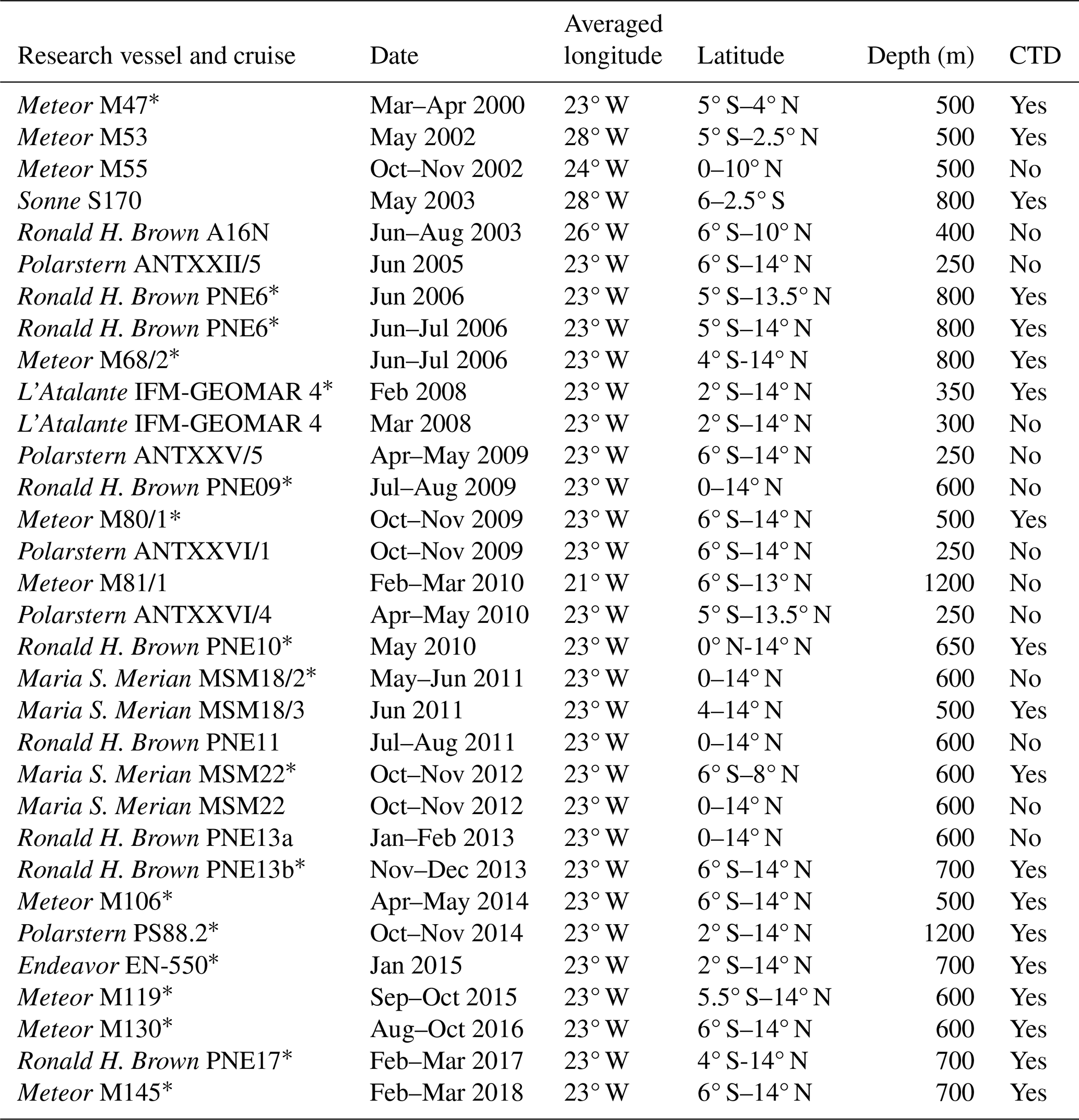
^* Cruises used to derive the buoyancy frequency profile at 0° N, 23° W.

Table A2 Meridional ship sections taken at 35° W from 1990 to 2006. For all sections, ADCP and hydrographic data are available. This dataset is from Hormann and Brandt (2007).

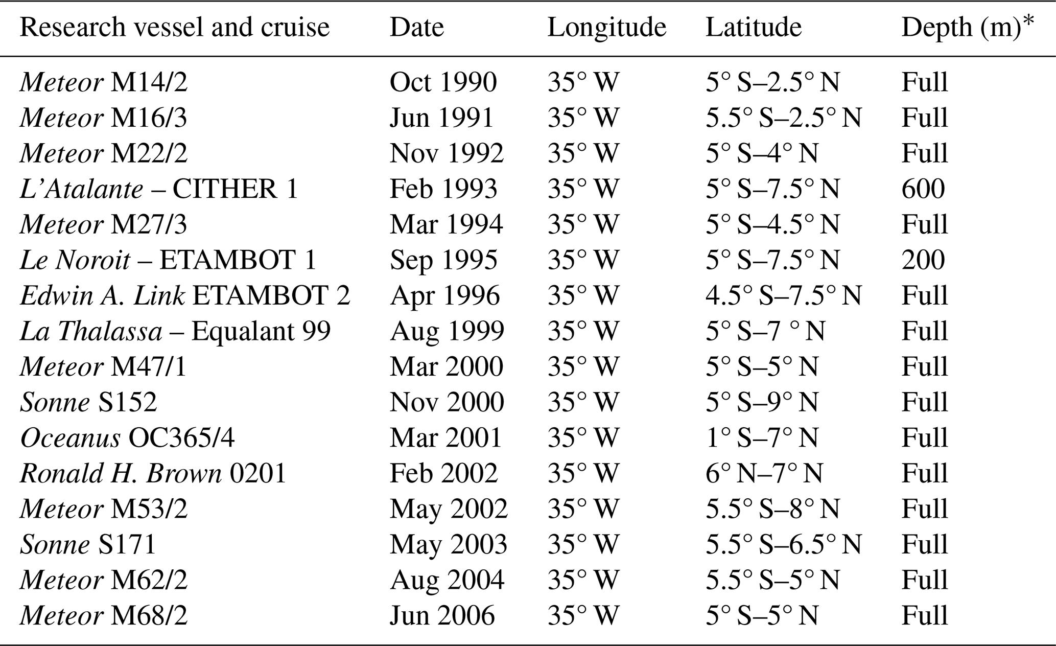
^* Depths marked as “full” span the entire water column.

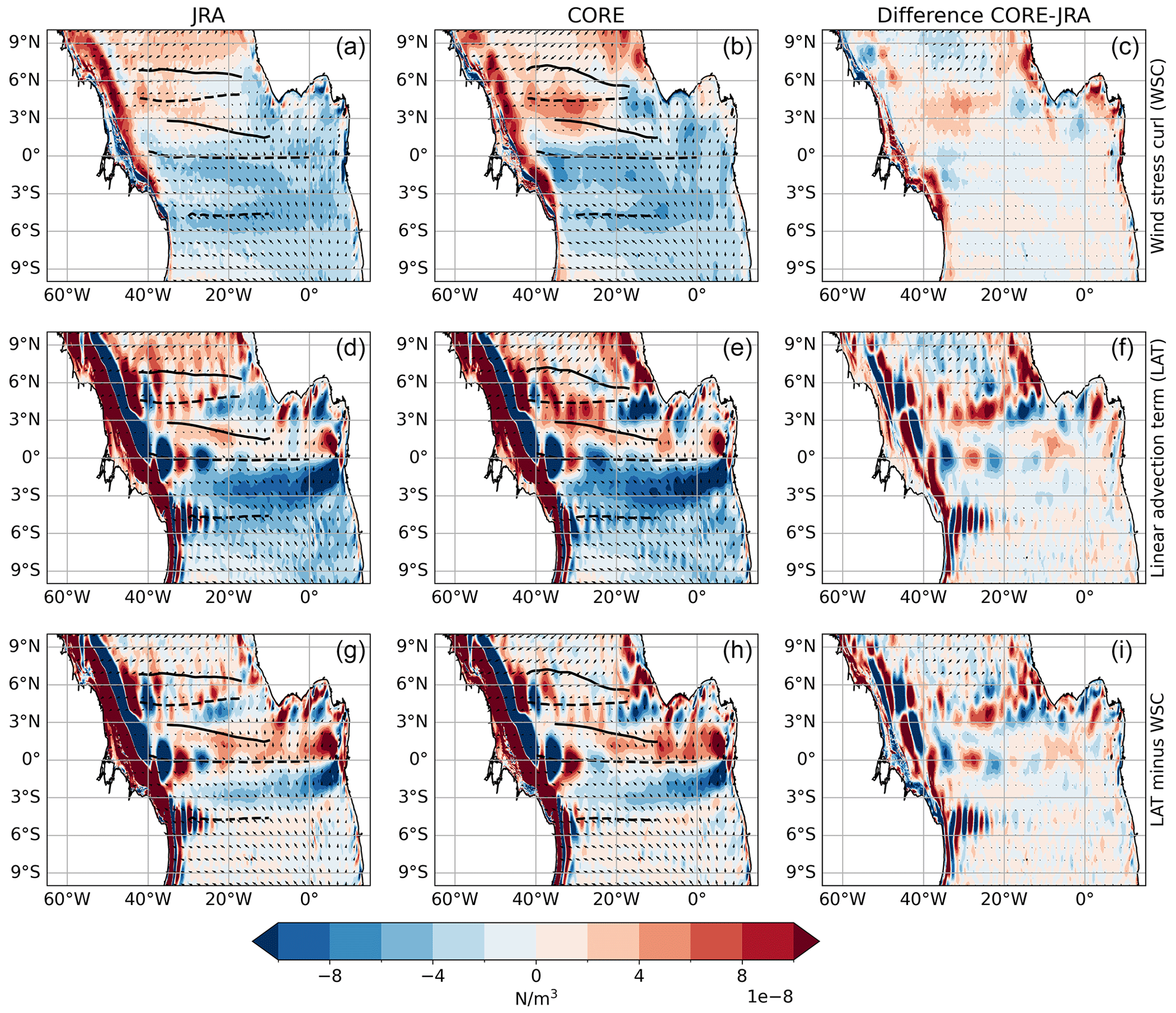
Figure A1 The 1980 to 2009 mean maps of wind stress curl (WSC; colour shading, a–c), wind stress (arrows), the linear advection term $\mathit{\beta }{\mathit{\rho }}_{\mathrm{0}}{\int }_{H=\mathrm{500}\mathrm{m}}^{\mathrm{0}}v\mathrm{d}z$ (LAT; colour shading, d–f) and the difference in the two terms (colour shading, g–i) calculated using JRA_sim (a, d, g), CORE_sim (b, e, h) and the difference between the two forcings (c, f, i). Under Sverdrup balance, LAT and WSC should be equal. Zonal black lines in mark the mean latitude (Y_CM, Eq. 1) of the simulated surface (solid) and subsurface (dashed) currents for the respective periods.

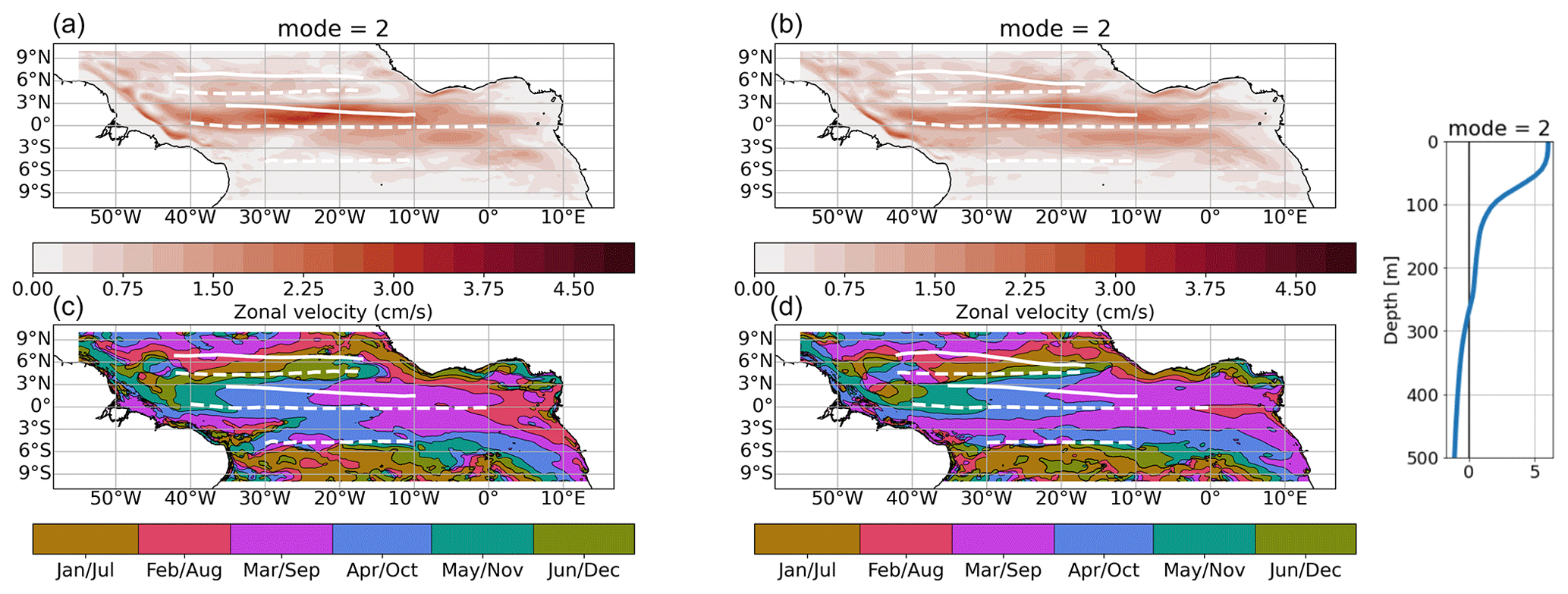
Figure A2 Amplitude (a, b) and phase (c, d) of the second baroclinic mode semi-annual cycle of zonal velocity from JRA_sim (a–c, 2000–2018) and CORE_sim (b, d, 1991–2009). To derive the 3D zonal velocity field associated with the specific baroclinic mode, the amplitudes must be multiplied by the corresponding vertical structure function shown on the right. The phase is given in the month of the year when maximum eastward velocity occurs at the surface. Zonal white lines mark the mean latitude (Y_CM; Eq. 2) of the simulated surface (solid) and subsurface (dashed) currents for the respective periods.

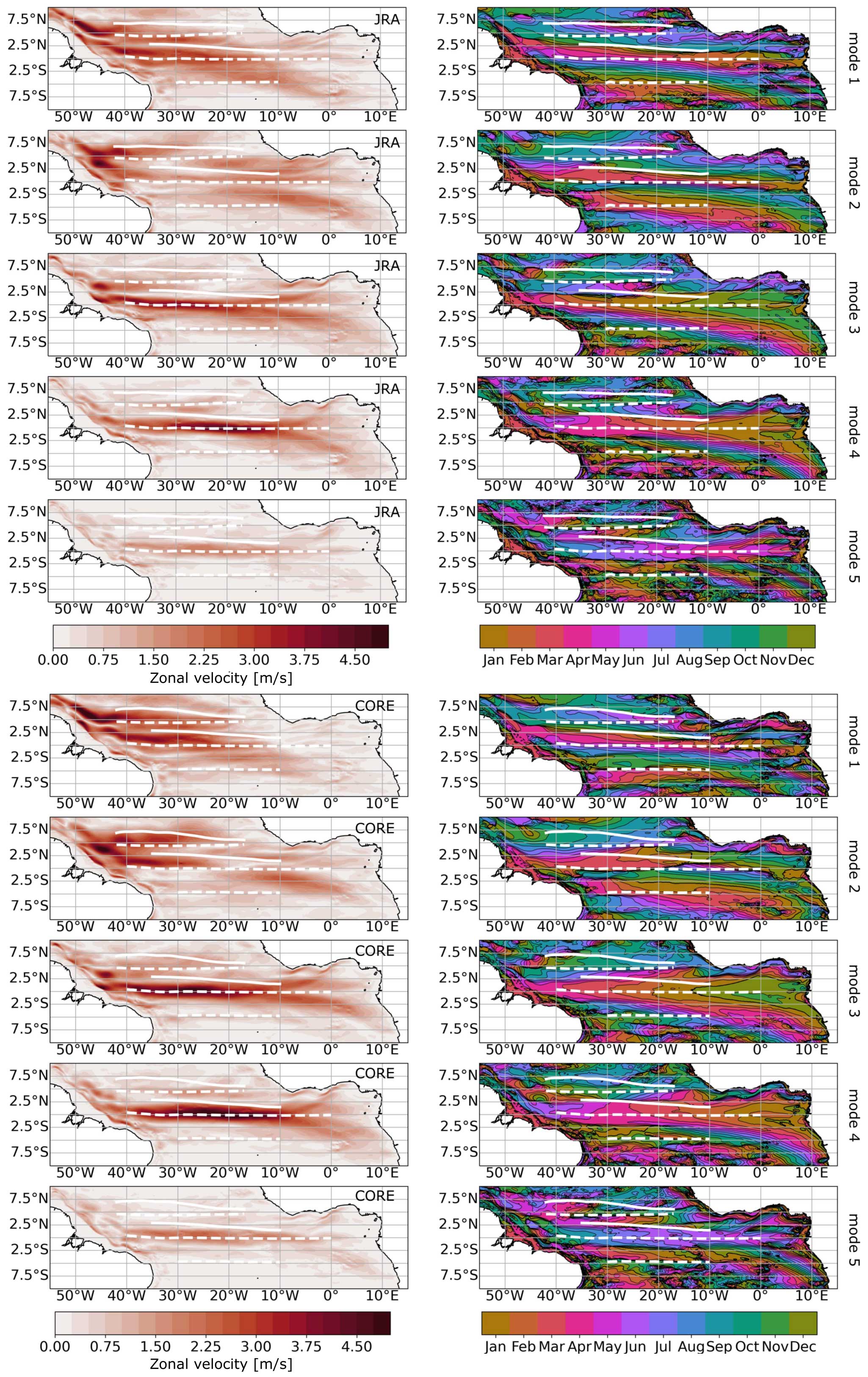
Figure A3 Amplitude (left) and phase (right) of first five baroclinic modes and the annual cycle of zonal velocity from JRA_sim and CORE_sim (1980–2009). To derive the 3D zonal velocity field associated with the specific baroclinic mode, the amplitudes must be multiplied by the corresponding vertical structure function. The phase is given in month of the year when maximum eastward velocity occurs at the surface. Zonal white lines mark the mean latitude (Y_CM; Eq. 2) of the simulated surface (solid) and subsurface (dashed) currents for the respective periods.

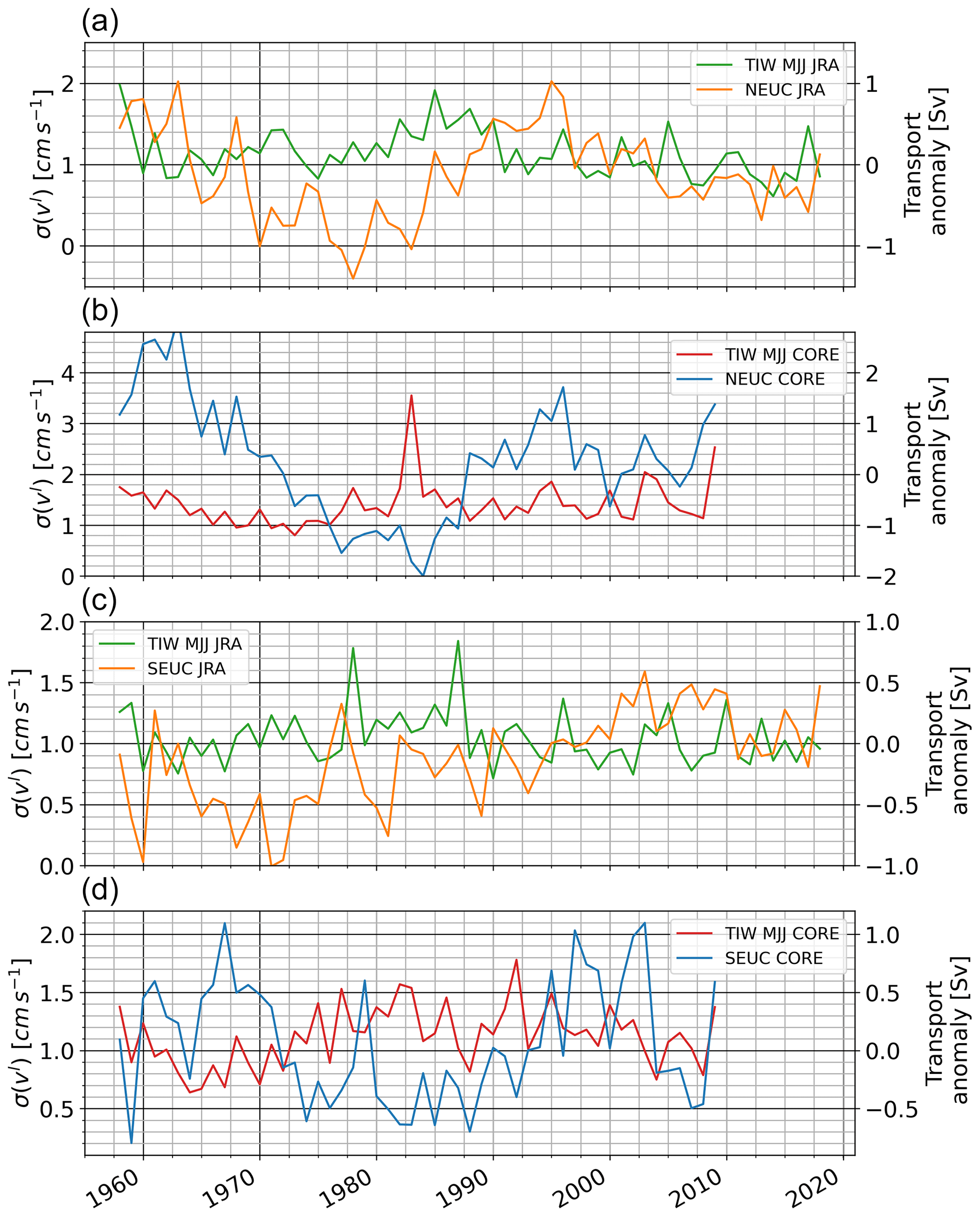
Figure A4 Long-term TIW activity shown as May–June averages of monthly standard deviation of band-pass-filtered meridional velocity at 160 m depth in JRA_sim (green lines) and CORE_sim (red lines) spatially averaged within the NEUC (a, b) and SEUC region (c, d). Also shown are the zonally averaged annual mean transport anomalies of the NEUC and SEUC in JRA_sim (orange lines) and CORE_sim (blue lines).

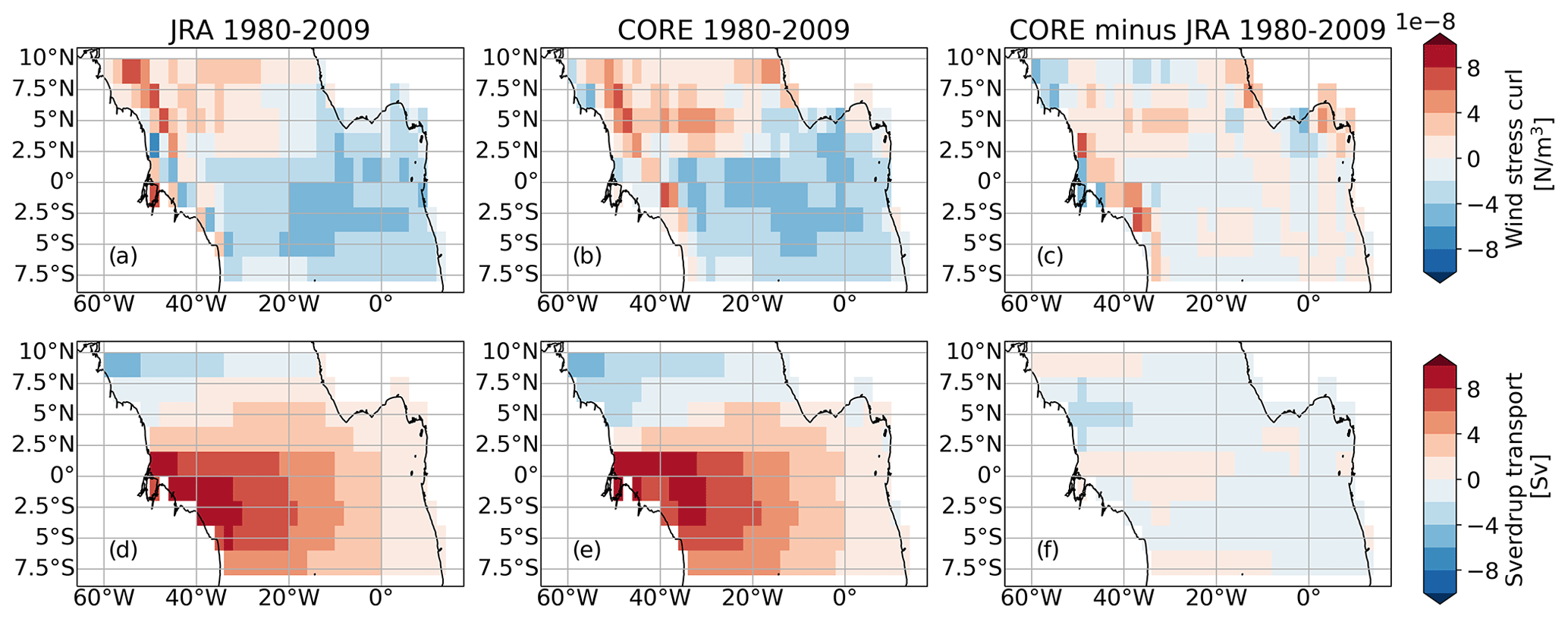
Figure A5 The 1980 to 2009 mean maps of wind stress curl (a–c) and Sverdrup transport (d–f) calculated from wind stress data averaged in 2° × 2° bins.