the Creative Commons Attribution 4.0 License.
the Creative Commons Attribution 4.0 License.
 | 21 Feb 2024
Linking satellites to genes with machine learning to estimate phytoplankton community structure from space
Roy El Hourany
Juan Pierella Karlusich
Lucie Zinger
Hubert Loisel
Chris Bowler
Ocean color remote sensing has been used for more than 2 decades to estimate primary productivity. Approaches have also been developed to disentangle phytoplankton community structure based on spectral data from space, in particular when combined with in situ measurements of photosynthetic pigments. Here, we propose a new ocean color algorithm to derive the relative cell abundance of seven phytoplankton groups, as well as their contribution to total chlorophyll a (Chl a) at the global scale. Our algorithm is based on machine learning and has been trained using remotely sensed parameters (reflectance, backscattering, and attenuation coefficients at different wavelengths, plus temperature and Chl a) combined with an omics-based biomarker developed using Tara Oceans data representing a single-copy gene encoding a component of the photosynthetic machinery that is present across all phytoplankton, including both prokaryotes and eukaryotes. It differs from previous methods which rely on diagnostic pigments to derive phytoplankton groups. Our methodology provides robust estimates of the phytoplankton community structure in terms of relative cell abundance and contribution to total Chl a concentration. The newly generated datasets yield complementary information about different aspects of phytoplankton that are valuable for assessing the contributions of different phytoplankton groups to primary productivity and inferring community assembly processes. This makes remote sensing observations excellent tools to collect essential biodiversity variables (EBVs) and provide a foundation for developing marine biodiversity forecasts.
- Article
(18295 KB) - Full-text XML
-
Supplement
(4892 KB) - BibTeX
- EndNote


The production of organic matter (i.e., productivity) in marine ecosystems relies largely on phytoplankton. These unicellular photosynthetic microorganisms are evolutionarily diverse and exhibit a wide range of cell morphologies, sizes, photosynthetic accessory pigments, elemental requirements, and biogeochemical and trophic functions (Pierella Karlusich et al., 2020). They play a key role in regulating ocean biogeochemistry (Fuhrman, 2009) and global climate, partly through the absorption of atmospheric CO2 and export of carbon to the deep ocean (Guidi et al., 2009; Tilman et al., 2014; Tara Ocean Foundation, 2022).
In order to investigate the potential impacts of environmental changes on marine ecosystem functioning (Ibarbalz et al., 2019; Henson et al., 2021), high-resolution, real-time, and global-scale data on phytoplankton community structure are required (Pereira et al., 2013). However, existing knowledge about the global distribution of phytoplankton communities from in situ observations is highly fragmented, spatially disparate, and temporally punctuated. It is furthermore limited by both the challenges of in situ data collection and the associated costs of measurement techniques, which range from microorganism imaging and flow cytometry to DNA sequencing (Hillebrand and Azovsky, 2001; Irigoien et al., 2004; Smith, 2007; Rodríguez-Ramos et al., 2015; Powell and Glazier, 2017; Righetti et al., 2019; Dutkiewicz et al., 2020; Pierella Karlusich et al., 2020).
Ocean color remote sensing offers an interesting alternative to map the global distribution of phytoplankton communities at the sea surface at a high spatiotemporal resolution. Since 1978, ocean color satellites have been used to observe the concentration of the main phytoplankton pigment, chlorophyll a (Chl a), considered a proxy for phytoplankton biomass (O'Reilly et al., 1998; Sathyendranath et al., 2014). Recently, ocean color data have also been used to gain information about phytoplankton communities, such as their size structure and their taxonomic or functional composition. This interest has facilitated the integration of the concept of phytoplankton functional types (PFTs) and taxonomic phytoplankton groups (PGs) into studies exploring various ecological and biogeochemical aspects (Le Quéré et al., 2005; Hood et al., 2006). PFTs refer to distinct categories associated with biogeochemical processes (e.g., silicifiers, calcifiers) and physiological adaptations to environmental factors (e.g., light, nutrients, turbulence) or to more practical categories identified through specific analytical techniques (e.g., pigment types) (IOCCG report no. 14). On the other hand, phytoplankton groups correspond to taxonomic classes (e.g., diatoms, haptophytes, cyanobacteria). It is important to note that phytoplankton from different taxonomic groups can perform the same ecosystem function; e.g., both diatoms and silicoflagellates can biosilicify but represent different taxonomic groups. Specialized algorithms applied to ocean color data have consequently been developed to detect specific taxa with distinctive optical characteristics (e.g., Brown, 1995; Iglesias-Rodríguez et al., 2002), the dominance of PFTs (e.g., Alvain et al., 2005), the relative abundance of PGs and size classes in terms of their contribution to Chl a (e.g., Hirata et al., 2011; Xi et al., 2020, 2021), and recently plankton assemblages and communities (e.g., Kaneko et al., 2023).
The diagnostic pigment analysis method (DPA; Vidussi et al., 2001) relies on the association of secondary phytoplankton pigments with different broad taxonomic phytoplankton groups. DPA classification was later refined by Uitz et al. (2006), who gave different weightings to the diagnostic pigments to retrieve three phytoplankton size classes (PSCs) from total Chl a. The advantage of this method is that phytoplankton pigments can be measured cost-effectively through high-performance liquid chromatography (HPLC). Today, large in situ HPLC datasets are available with broad spatial and temporal coverage. These HPLC datasets have enabled the development of several DPA-based ocean color algorithms, which has made it possible to evaluate the abundance of different phytoplankton groups and size classes from ocean color satellite data (e.g., Uitz et al., 2006; Hirata et al., 2008, 2011; Soppa et al., 2014; Di Cicco et al., 2017; Organelli et al., 2013; El Hourany et al., 2019a, b; Brewin et al., 2010; Xi et al., 2021). However, the limitation of the DPA approach is that it is associated with large uncertainties in the classification of phytoplankton due to the presence of some pigments in different phytoplankton taxa and cell size classes, which also vary with acclimation to light, temperature, and nutrient availability (Brewin et al., 2015; Chase et al., 2020).
In this work, we propose an alternate approach to develop an ocean color algorithm for phytoplankton group detection from in situ metagenomic observations. The approach is ground-truthed on data collected by Tara Oceans, which constitutes the most comprehensive and harmonized molecular dataset available on phytoplankton taxonomic community structure on a global scale. More specifically, we used metagenomics reads to extract the global-scale distribution and abundance of the single-copy gene psbO, which is present across all phytoplankton groups and provides an unbiased picture of phytoplankton cell abundances (Pierella Karlusich et al., 2022). We used these data, together with satellite-derived optical, physical, and biogeochemical parameters, to train an unsupervised machine learning algorithm able to discern the nonlinear relationship between phytoplankton taxonomic community structure and data derived from satellites. This new algorithm allowed us to derive the spatiotemporal variability of seven PGs between 1997 and 2021. We then compared the performance of this new algorithm with that of two previous DPA-based algorithms (El Hourany et al., 2019a; Xi et al., 2021).
In this section, we present the datasets that were used for training the algorithm and for evaluating the outputs. The input dataset includes the in situ distribution and abundance of phytoplankton groups inferred from metagenomics data from Tara Oceans and their associated satellite matchups. The outputs of the new algorithm are compared to a global dataset of in situ HPLC diagnostic pigments, as well as with estimates from two DPA-based remote sensing algorithms.
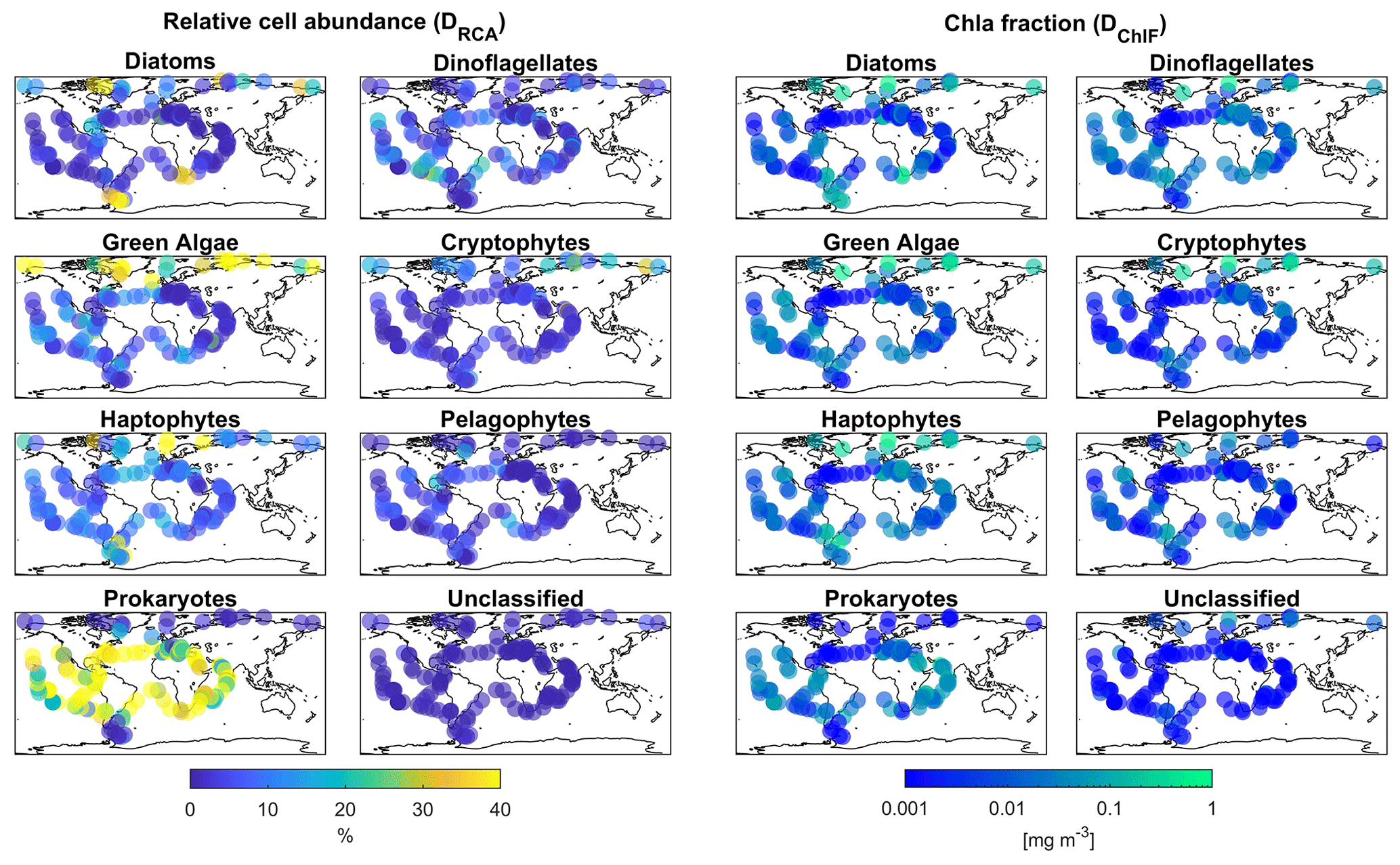
Figure 1Global biogeographical patterns of marine phytoplankton relative cell abundance and Chl a fraction per group based on psbO reads obtained from metagenomes from seawater samples collected during the Tara Oceans expeditions. Two sub-datasets are represented in this figure; the first, DRCA, is composed of psbO-derived relative cell abundance, and the second, DChlF, psbO-derived Chl a fraction per phytoplankton group.
2.1 Input dataset
2.1.1 Metagenomic read abundance of the psbO gene
The psbO gene encodes the manganese-stabilizing protein of around 270 amino acids, which constitutes a core subunit of photosystem II (PSII) and is unique to organisms carrying out oxygenic photosynthesis. The psbO gene is a single-copy gene in the vast majority of eukaryotes and prokaryotes. We used psbO reads from the metagenomes generated by the Tara Oceans expedition as a proxy for phytoplankton relative cell abundance (Pierella Karlusich et al., 2022). Among the 210 Tara Oceans stations, 145 stations sampled psbO reads in different ocean regimes from oligotrophic to eutrophic waters (Chl a from 0.01 to 10 mg m−3, median at 0.3 mg m−3) from 2009 to 2013. Seawater samples were filtered in order to differentiate five planktonic size fractions (0.22–3, 0.8–5, 5–20, 20–180, 180–2000 µm). For the purpose of this study, we pooled the five size fractions into a single aggregated sample.
The psbO data enabled us to taxonomically differentiate seven phytoplankton groups: diatoms, dinoflagellates, green algae, haptophytes, pelagophytes, cryptophytes, and prokaryotes (cyanobacteria) (Fig. 1). The psbO read abundances of these seven groups are expressed as relative phytoplankton cell abundance (%). Phytoplankton that were not assigned to any of these seven groups (unclassified) represented less than 5 % of the total relative cell abundance among all size classes.
The psbO measurements are proxies for relative cell abundance since this protein-encoding gene is generally present as a single copy and is found in all phytoplankton groups. For example, if we take a micro-sized diatom compared to a pico-sized Synechococcus, both have one psbO gene and are therefore counted as one within the psbO quantification. However, we know that a diatom's Chl a content is significantly greater than that of Synechococcus (Agustí, 1991; Fujiki and Taguchi, 2002; Dairiki et al., 2020; Bock et al., 2022). This is where the conversion via size-dependent weights is essential in the case of Chl a content estimation.
We should note, however, that filters may retain cells smaller than the nominal pore size because of net clogging, being trapped in fecal pellets, and being present as symbioses and colonies. This has been observed with prokaryotic pico-sized cells such as Synechococcus and Prochloroccocus being overrepresented in the 180–2000 µm size fraction (Fig. 2). To minimize this impact, we based our size weighting on four size fractions, while excluding the 180–2000 µm size range. Chl a fraction per group is expressed as follows:
where is the psbO read abundance for a specific phytoplankton group (PG) and for one of the four size fractions (s), and size corresponds to the mid-value of the corresponding size range, following the protocol in Sommeria-Klein et al. (2021), i.e., ×0.9 for the [0.6–1.2] size class, ×2.9 for the [0.8–5] size class, ×12.5 for the [5–20] size class, and ×100 for the [20–180] size class. Applying Eq. (1) pools all size fractions per group while considering the psbO read values and the size factors mentioned above.
There are hence two levels of information derived from the molecular dataset: relative abundance of psbO reads as a proxy for relative cell abundance and the fraction of Chl a that each group represents. Both types of information have different implications. Chl a is often used as a proxy for biomass, which is a relevant parameter for energy and matter fluxes (e.g., food webs, biogeochemical cycles), while cell abundance corresponds to species abundance for unicellular organisms, which is an important measure for inferring community assembly processes.
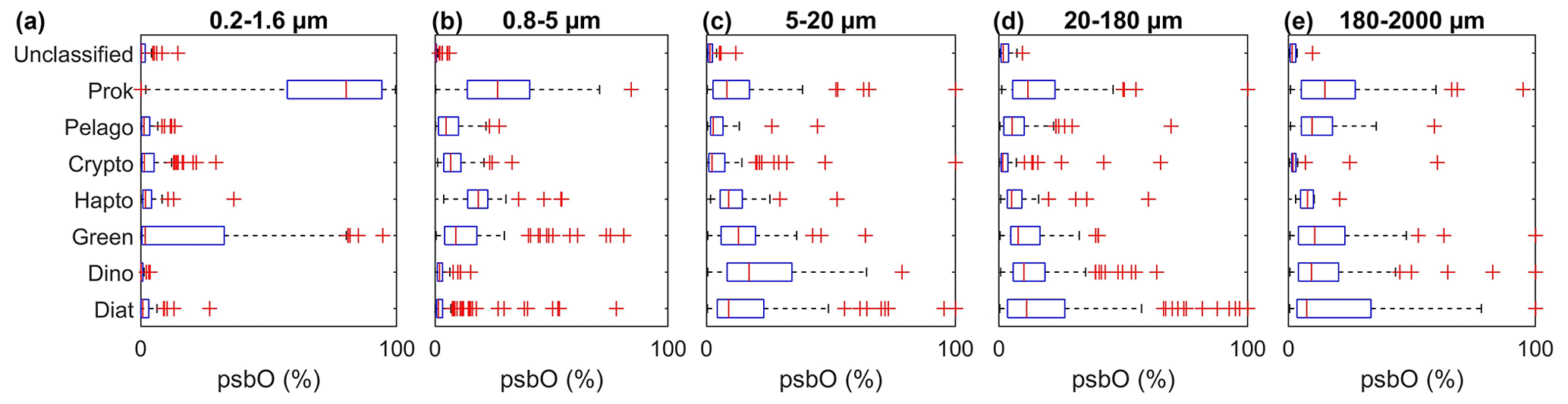
Figure 2Relative abundance of psbO reads as a proxy for phytoplankton group cell abundance observed in each size fraction. The box plots represent the distribution of each group, and each panel shows the different size fractions. The equivalent plots for the psbO read values normalized by sequencing depth are displayed in the Supplement in Fig. S1.
2.1.2 Satellite datasets
We used ocean color products from the GlobColour project (R2019, full archive reprocessed, 2020) from 1997 to the present day, downloaded from the GlobColour portal. These products were constructed by merging data from various satellite sensors: Sea-viewing Wide Field-of-view Sensor (SeaWiFS), Moderate Resolution Imaging Spectroradiometer (MODIS), Visible Infrared Imaging Radiometer Suite (VIIRS), Medium Resolution Imaging Spectrometer (MERIS), and Ocean and Land Colour Instrument (OLCI). We used 16 GlobColour products: chlorophyll a concentration (Chl a, product name: CHL1-AVW), remote sensing reflectances (Rrs) at 11 wavelengths (412, 443, 469, 490, 510, 531, 547, 555, 620, 645, and 670 nm), light attenuation coefficient at 490 nm (Kd490), photosynthetically available radiation (PAR), normalized fluorescence light height (NFLH), and particulate backscattering at 443 nm (bbp). These products have daily and 4 km spatiotemporal resolution. In addition, we used the Climate Change Initiative (CCI) sea surface temperature (SST) product at 4 km resolution and daily frequency distributed by the Copernicus Marine Services (CMEMS) portal.
2.2 HPLC datasets
To compare psbO-derived phytoplankton group distributions with more conventional DPA-based products, we compiled a global HPLC dataset regrouping 12 000 HPLC observations from several HPLC datasets between 1997 and 2014 (Fig. 3, Table S1): MAREDAT, NOMAD, SeaBASS, AESOP-CSIRO, and other oceanographic campaigns including GeP&Co, Polarstern, BROKE-West, and SAZ-Sense Voyage (Werdell et al., 2003; Werdell and Bailey, 2005; Dandonneau et al., 2004; Bracher, 2015a, b, c; Peloquin et al., 2013; Wright et al., 2010; de Salas et al., 2011). This HPLC dataset was collocated with satellite GlobColour and the CCI SST product matchups. It depicts the abundance of the pigments most widely used to identify major phytoplankton groups: fucoxanthin (Fuco), peridinin (Perid), alloxanthin (Allo), zeaxanthin (Zea), chlorophyll b (Chl b), 19′-hexanoyloxyfucoxanthin (19HF), and 19′-butanoyloxyfucoxanthin (19BF) (Table 1). To estimate the Chl a fraction for each phytoplankton group, namely diatoms, dinoflagellates, haptophytes, green algae, cryptophytes, pelgophytes, and prokaryotes, diagnostic pigments were used. The Chl a fraction per group is expressed by
where a is a coefficient associated with a diagnostic pigment (DP) for a specific PG.
Four sets of coefficients a are proposed for a global ocean application and are presented in Table 1 (Uitz et al., 2006; Soppa et al., 2014; Brewin et al., 2015; Losa et al., 2017). An examination of the values assigned to the coefficients by these four studies reveals disparities that do not consistently align across all pigments. Notably, while the coefficients for diatoms exhibit similarity across the four sets, differences arise. For instance, in the case of dinoflagellates, only Uitz et al. (2006) and Brewin et al. (2015) show close coefficients associated with Perid, while in the case of haptophytes, Brewin et al. (2015), Soppa et al. (2014), and Losa et al. (2017) estimate close coefficients attributed to 19HF. The discrepancies can be attributed to variations in the datasets utilized for coefficient estimation and differences in the methodologies employed. We averaged the output of the four sets of coefficients to increase the robustness of the results while considering the different outputs of the utilization of these coefficients.
Simultaneously, Tara Oceans HPLC measurements (Pesant et al., 2015), which are available for the same stations and sampling time as for psbO, were considered to evaluate the correspondence between pigments and psbO-derived phytoplankton groups.
Table 1Phytoplankton groups and size classes associated with their diagnostic pigments and coefficients α. Major phytoplankton groups, emphasized in bold, serve to label the outputs resulting from the application of coefficient α to the respective diagnostic pigment.
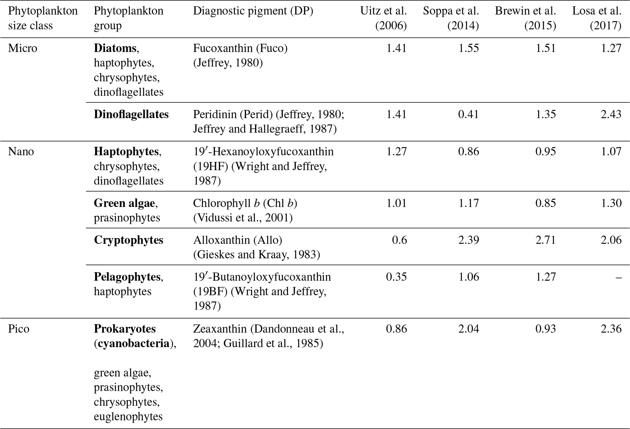
Coefficients are based on the global HPLC dataset corresponding to the sum of the weighted diagnostic pigments to the total Chl a; Chl DP.
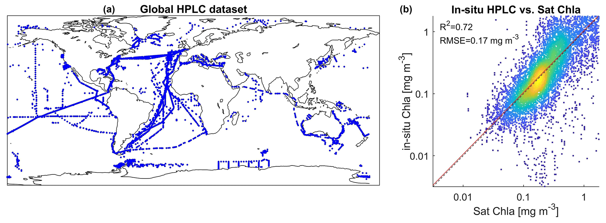
Figure 3(a) Geographical location of the global HPLC dataset stations regrouping observations from 1997 and 2014. Panel (b) represents a comparison between in situ HPLC Chl a measurement and its matchup using the GlobColour Chl a product.
2.3 Phytoplankton group satellite products
In order to compare the outputs of our method to those of existing DPA-based remote sensing algorithms, we used two previously published algorithms.
2.3.1 CMEMS phytoplankton Chl a fraction
This daily GlobColour product contains the concentration of each phytoplankton group (expressed in terms of Chl a concentration fraction) based on the Xi et al. (2021) algorithm from 2002 to the present at the global scale and with a 4 km resolution. This algorithm estimates the Chl a concentration of diatoms, dinoflagellates, haptophytes, green algae, and prokaryotes. The algorithm was implemented with HPLC-based phytoplankton groups using the DPA approach (Soppa et al., 2014) merged to ocean color (OC) Rrs products (412, 443, 490, 510, 531, 547, 555, 670, and 678 nm) and accounting for the influence of SST on the derived PG quantities (product number: OCEANCOLOUR_GLO_BGC_L3_MY_009_103).
2.3.2 SOM phytoplankton pigments
SOM-Pigments (El Hourany et al., 2019a) is a machine-learning-based algorithm that allows the estimation of phytoplankton pigment concentrations in oceanic waters from satellite ocean color data (chlca, Rrs at four wavelengths: 412, 443, 490, and 555 nm) and SST. This algorithm is based on the use of self-organizing maps (SOMs) and an unsupervised neural network, and it was calibrated using the HPLC dataset described above.
The SOM-Pigments algorithm applied to GlobColour products allows estimating the daily concentration of 10 phytoplankton pigments (chlorophyll a – Chl a, divinyl-chlorophyll a – DVChl a, chlorophyll b – Chl b, divinyl-chlorophyll b – DVChl b, 19′exfucoxanthin – 19HF, 19′butfucoxanthin – 19BF, fucoxanthin – Fuco, peridinin – Perid, alloxanthin – Allo, zeaxanthin – Zea) at the global scale from 1997 to the present with a resolution of 4 km. We then used the coefficients in Table 1 of Uitz et al. (2006), Soppa et al. (2014), and Brewin et al. (2015) to convert pigments into the Chl a concentration of five phytoplankton groups, namely diatoms, dinoflagellates, haptophytes, green algae, and prokaryotes.
The algorithm to estimate phytoplankton groups from satellite data was built using SOM (Kohonen, 2013) and topology-constrained organization. This allowed us to confirm the nonlinear relationships between phytoplankton group composition and satellite data through topology conservation. Next, we used the ascending hierarchical clustering algorithm to identify the large-scale patterns generated by SOM. This allowed us to emphasize the predominant data structure learned by SOM and to characterize phytoplankton biomes. The steps of the training and operational phase of the SOM methodology are illustrated in flowcharts found in the Supplement (Figs. S2–S4). Finally, to characterize the differences between the DPA- and psbO-based approaches, we used random forest models to highlight the cumulative importance of a pigment composition to estimate a phytoplankton group abundance. In the following section, each methodology and algorithm is explained in detail.
3.1 Structure of the training and test databases
The initial dataset (D) consists of the 145 Tara Oceans observations of psbO relative abundance of the seven defined phytoplankton groups, the Chl a fraction per group, and the associated matchups of 21 satellite-derived parameters (Chl a, SST, Rrs at 15 wavelengths from 412 to 709 nm, NFLH, Kd at 490 m, PAR, and bbp at 443 nm). The unclassified phytoplankton fraction was also considered, despite negligible values, to ensure coherence of the total phytoplankton pool. To extract the matchup for a given observation, a 3×3 pixel box was employed, centered around the observation's coordinates on the same day. The average of the non-outlier pixels was computed. If this approach was unproductive due to fewer than four valid pixels within the 3×3 box or the absence of any pixel, a 3×3 pixel extraction was performed for the adjacent days (+1 and −1) (El Hourany et al., 2019a, b). Following these matchup exercises, we performed a baseline comparison between in situ Chl a and satellite-derived Chl a. This comparison is deemed satisfactory, with an average error rate of 33 %.
We built two sub-datasets, the first (DRCA) relating psbO-derived relative cell abundance of the seven defined phytoplankton groups to the 17 satellite-derived parameters and the second (DChlF) joining psbO-derived Chl a fraction per phytoplankton group and the same 17 satellite-derived parameters. We then constructed two algorithms using either DRCA or DChlF, both based on the same SOM methodology described below. Following the positioning of Tara Oceans stations and the distribution of Chl a values within both datasets (Figs. S5 and S6), both algorithms are suitable for case 1 water applications (i.e., open ocean).
The rationale behind this is that the phytoplankton community should be treated as a whole; consequently, the variability of each phytoplankton group is dependent on each other in a relative way. DRCA and DChlF both present missing values (Table 2), most likely due to cloud coverage, coastal proximity, and/or ice presence. In situ psbO-based observations also contained missing values due to an absence of certain measurements at a given station. Since the in situ dataset contains a low number of observations (145 stations), every observation is valuable. In order to overcome the several limitations faced with this training dataset, we used the SOM algorithm that can deal with missing values and allow a robust generalization in the case of limited observations (Jouini et al., 2013). Before applying the SOM, we ensured that all variables, phytoplankton observations, and satellite parameters were weighted alike while normalizing their values by their variance.
Table 2Percentage of missing values within the initial database.

3.2 Self-organizing map applied to Tara Oceans psbO data
3.2.1 General concept of SOM
The SOM algorithm is utilized for clustering multidimensional databases by assigning them to classes represented by a fixed network of neurons known as the self-organizing map (SOM). The SOM consists of a rectangular grid of p×q neurons and defines a discrete distance between neurons, enabling the partitioning of the dataset. Each cluster is associated with a neuron and represented by a prototype vector. Observations in the dataset are assigned to the nearest neuron based on the Euclidean norm. A key feature of SOM is its ability to provide topological ordering, where close neurons on the map correspond to similar observations in the data space. The estimation of a neuron's vector and the topological order are determined through a minimization process of a cost function that depends on the distance between the neuron and its assigned observation. SOMs have been widely employed to complete missing data, utilizing the truncated distance (Folguera et al., 2015; Charantonis et al., 2015; Saitoh, 2016; Rejeb et al., 2022). The truncated distance is defined as a modification of the standard Euclidean distance between two observations that accounts only for the existing components of the vectors. This modification of the distance measure allows for the comparison of observations with incomplete information by considering only the existing components and effectively handling missing data. The SOM algorithm can then use this truncated distance measure in its learning process to complete missing data and integrate incomplete information, enabling more robust analysis and visualization of the data.
3.2.2 Training phase
Briefly, we first split the Tara Oceans psbO datasets so as to obtain 80 % of the data to train the SOM and 20 % of the data as a test set, the latter consisting of 30 observations with complete psbO information. We did this separately for DRCA and DChlF sub-datasets so as to generate SOMRCA, which stands for the algorithm specialized in relative cell abundance estimation, and SOMChlF for the algorithm specialized in Chl a fraction per phytoplankton group.
During the SOM training, different combinations of satellite variables were used to determine the best set of variables to estimate the seven phytoplankton groups in terms of relative cell abundance and Chl a fraction. For each combination of variables, we increased the number of neurons from 10 to 1000 neurons, with an interval of 10 neurons, to determine the optimal size of the SOM. For each SOM obtained, we quantified quantization and topographic errors. The quantization error represents the difference between an observation and its closest neuron. This error is monitored during the training procedure until it reaches stability at a minimum value with increasing training epochs. This is where the training should stop to prevent overfitting. The quantization error is expressed as follows:
where xi is the vector of an input observation i, wci is the vector of the closest neuron c of a sample xi, and n is the number of observations.
However, the topographic error is a representation of having, for each observation of the database, distant first and second best-matching neurons and is expressed as follows:
where d(xi)=1 if the first and second closest neurons to xi are not adjacent; otherwise, d(xi)=0.
Minimizing this quantity is important to ensure the preservation of the topological order within the SOM with an increasing number of interpolated neurons. A leave-one-out cross-validation procedure was performed to assign three performance metrics to help choose the best combination of SOM size and satellite variables: regression coefficient (R2) and root mean squared error (RMSE). One should note that, for SOMChlF, the R2 was calculated using log-transformed Chl a values, and RMSE was calculated using non-transformed Chl a values. At each iteration of the cross-validation procedure, we randomly chose one observation as a test, whereas the other observations served to train the SOM with the given grid size. We calculated the closest neuron to the test observation based on its satellite variables only and associated these latter with the neuron's vector for the seven phytoplankton groups. When all the observations were used as a test, we calculated a mean R2 and an RMSE associated with the given size map, while comparing the estimated and observed phytoplankton group values. The best SOM configuration and variable combination are based on an optimum where te, qe, and the RMSE are in low ranges while avoiding overfitting. The chosen SOM was tested using the 20 % test set, providing independent performance metrics to evaluate the generalization of the chosen SOM. As a result, we present in the paper the performance metrics of the chosen SOM configuration based on the cross-validation procedure and the test set.
The optimal combination of satellite parameters for the SOMRCA and SOMChlF algorithms was determined to be Chl a, SST, Rrs at four wavelengths (412, 443, 490, and 555 nm), bbp, and Kd490. The grid size for SOMRCA was set at 242 neurons, while SOMChlF had a grid size of 222 neurons. This selection was based on several factors, including a high regression coefficient between estimated and observed phytoplankton values, low error values of quantization and topographic error, and a low global RMSE encompassing all phytoplankton groups. The choice of Rrs bands aligns with previous work conducted on the PHYSAT method by Alvain et al. (2005) and Ben Mustapha et al. (2013). The PHYSAT method utilizes water-leaving radiance anomalies in the same four selected bands to identify dominant phytoplankton functional types. In the clear open ocean, the information contained in the remote sensing reflectance (Rrs) bands beyond 555 nm is limited due to the strong absorption by water (Torrecilla et al., 2011; Taylor et al., 2011). It should be noted that the Rrs bands selected are commonly measured by all sensors used to build the Rrs product of GlobColour. This overlap of different sensors enhances data availability and coverage, thus increasing the importance of these Rrs bands within the initial dataset.
Through the iterative training process described above, the results show a significant increase in the general performance of the method when the number of neurons increases to a certain extent (Fig. 4). Using a number of neurons larger than the training dataset still allows a refined discretization. In this case, some neurons will capture a sample of the database, which permits defining a referent vector for these neurons. When the neuron did not capture any data observation, the discrete distance between the neighboring neurons was used to determine the referent vector w of each neuron that did not capture any data (Sarzeaud and Stephan, 2000; El Hourany et al., 2019a). This leads to preserving the topological order provided by new interpolated neurons. However, the quantization error’s lowest values above 350 neurons might indicate overfitting.
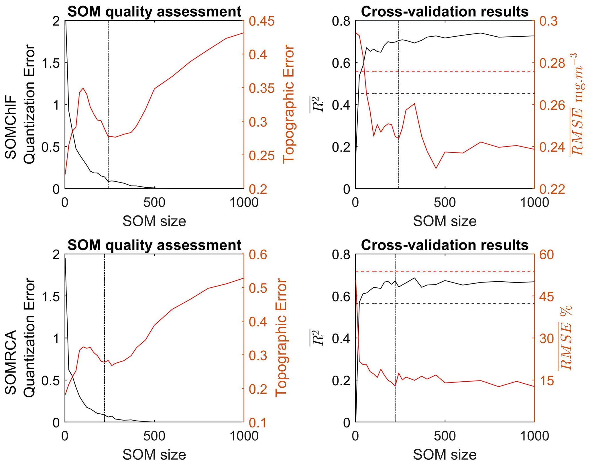
Figure 4Quality assessment based on the quantization and topographic error related to the training of SOMChlF and SOMRCA as a function of increasing SOM size (number of neurons) using Chl a, SST, Rrs at four wavelengths (412, 443, 490, and 555 nm), bbp, and Kd490. In parallel, the average regression coefficient and the root mean squared error as a function of increasing SOM size were calculated through a “leave-one-out” cross-validation procedure. The dashed black and red lines respectively correspond to the R2 and the RMSE using the K-nearest neighbor algorithm. Finally, the dotted lines correspond to the chosen SOM size for SOMChlF = 242 neurons and SOMRCA = 222 neurons.
3.2.3 Operational phase
During the operational phase, we estimated the phytoplankton group variability using the best combination of satellite parameters. The set of parameters of a pixel was projected onto the SOM. In doing so, the parameters at each pixel were normalized by the variance of that same parameter within the initial training dataset to maintain an equal weight among the parameters and were assigned with the closest best-matching neuron using the truncated distance. At the end of the assignment phase, each pixel was associated with a referent vector corresponding to the best-matching neuron, which includes the seven phytoplankton groups as a function of relative cell abundance in the case of SOMRCA or Chl a fraction in the case of SOMChlF. Since the training was undertaken for the whole phytoplankton community at once, alongside the total Chl a information, the SOM allows the inherent structure of the data to be preserved.
For this phase, level-3 mapped 4 km daily images were used to estimate the phytoplankton groups at the same spatiotemporal resolution.
3.2.4 Masking and uncertainty evaluation
Given that our initial dataset is of limited size, it is possible that it does not contain certain naturally occurring cases. In order to prevent abnormal predictions for cases not observed in the initial dataset, we conducted a quality evaluation of the method's output. This evaluation involved quantifying a reliability index by comparing the set of satellite parameter values at a particular pixel with the values of the same parameters in the initial dataset. If a satellite variable's value fell outside the range defined within the initial dataset by the mean value of the same variable’s distribution plus or minus 2 standard deviations, it was considered distant. This evaluation was performed for all satellite variables per pixel, and the reliability index was determined by dividing the number of accepted variables by the total number of existing variables. A higher reliability index indicates greater reliability of the method, while regions with lower reliability index values require additional attention.
In the context of the global ocean, numerous uncertainties are associated with in situ measurements, model parameterization, satellite parameters, and regions. The SOM algorithm is known to effectively reduce noise and mitigate the impact of uncertainties within the dataset (da Silva and Costa, 2013). However, the main source of uncertainty in the estimation process stems from selecting the best-matching neuron. This involves finding and associating the closest neuron in the SOM with a new or unfamiliar observation, such as a satellite pixel. Due to the topology conservation, a pixel could be assigned to several close neurons, forming a neighborhood along a distance gradient. Consequently, a single satellite observation can represent various probabilities of phytoplankton group combinations influenced, to a certain extent, by the uncertainties of the satellite parameter.
To account for uncertainties in the estimations, we opted to associate each pixel and phytoplankton group (based on relative cell abundance or Chl a fraction) with a weighted standard deviation derived from the values of the 10 closest neurons. The weights were determined by the distances between the first 10 matching neurons and the pixel. This approach allowed us to incorporate uncertainties into the assignment process and provide a confidence measure for each pixel's assignment. By considering both the reliability index and the weighted standard deviation, we could assess the influence of uncertainties in the satellite variables.
However, we should acknowledge the importance of addressing the uncertainties in the psbO measurements and their potential impacts on the algorithm's outputs, which are not taken into account in this study. This exclusion is primarily due to the absence of a comprehensive framework that accounts for all the associated steps in the quantification of psbO, including aspects such as filtration, extraction, and the accuracy of psbO analysis. Pierella Karlusich et al. (2022) conducted a thorough comparative study, evaluating psbO quantities against data obtained from confocal and optical microscopy, as well as cytometry, revealing agreement of 70 % (Spearman's rho = 0.64–0.71, p value < 0.001). However, it is essential to recognize that like psbO, every quantification method is subject to uncertainties stemming from the various steps of the quantification process, emphasizing the necessity of comprehensive assessments within every in situ measurement protocol.
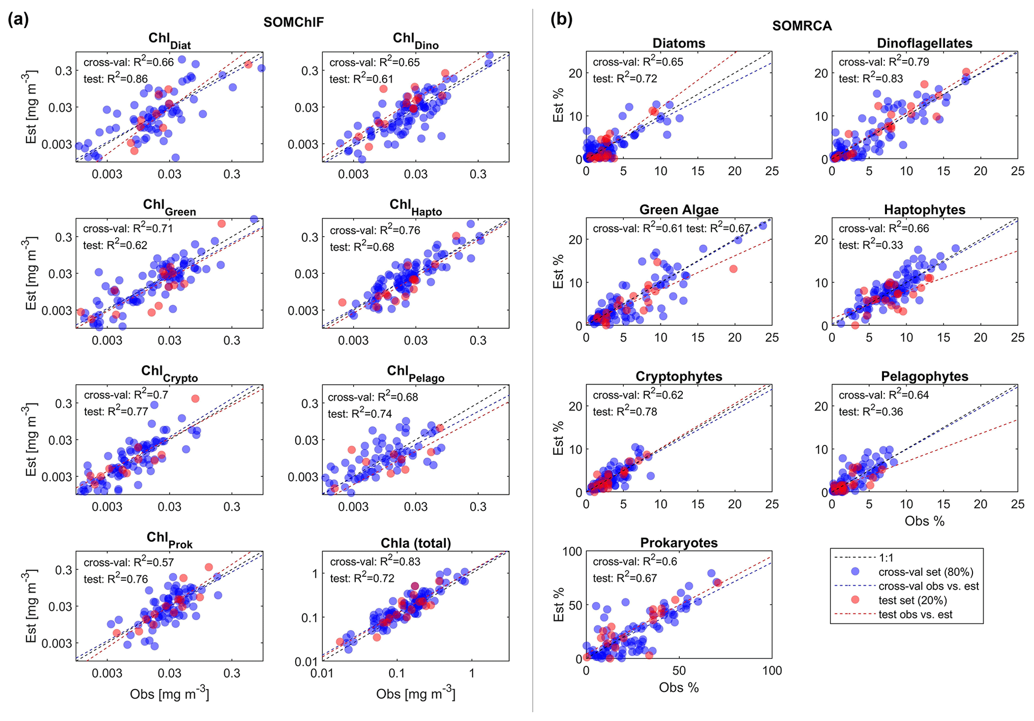
Figure 5Results of the two-step cross-validation (blue) and test (red) procedures for SOMChlF (a) and SOMRCA (b) with the chosen best combination of satellite parameters and a SOM grid, respectively, of 242 and 222 neurons. From the initial dataset consisting of 145 observations, two sets were split: 80 % to be used in a one-leave-out cross-validation procedure and 20 % as an independent test. For the cross-validation, each observation among the 115 observations was used iteratively as a training set and as a test set until all observations served as tests (blue dots). This procedure was used to identify the best satellite combination and SOM grid size. Finally, the remaining 30 observations were used as a test to evaluate the generalization capacity of the SOM with the chosen configuration (red dots). One should note that, for SOMChlF, the R2 was calculated using log-transformed Chl a values. For complete evaluation metrics refer to Table 3.
3.3 Characterization of phytoplankton biomes
To emphasize the predominant data structure learned by SOMChlF, the ascending hierarchical clustering algorithm (AHC) was used to characterize phytoplankton biomes on the basis of their Chl a fractions (a proxy for a phytoplankton group's biomass) and optical signature.
The AHC is a bottom-up clustering algorithm. The AHC starts with individuals and combines them according to their similarity (with respect to the chosen distance) to obtain new clusters. The exact number of biomes is not known a priori, but at the end of the SOM + AHC procedure, several possibilities of a number of clusters to be taken into account were revealed. A compromise was made between the number of clusters we could explain from a physical point of view and the number of clusters for which we needed to include the maximum information embedded in the dataset. This procedure has been used with success in several studies (Reygondeau et al., 2014; Richardson et al., 2003; Rossi et al., 2014; Sawadogo et al., 2009; El Hourany et al., 2021). At the end of the AHC clustering phase, each neuron of the SOMChlF was associated with a cluster. The association of several neurons in a cluster allows us to identify common phytoplankton community structures and therefore characterize phytoplankton biomes. Upon applying SOMChlF as described in the operational phase section, each pixel of a satellite image could be associated with a cluster.
3.4 Evaluation of pigments to estimate phytoplankton groups
Each phytoplankton group's psbO abundance was associated with its corresponding HPLC pigment measurements performed for the same Tara Oceans station. The ability of pigments to predict a specific phytoplankton group was evaluated using a bagged random forest algorithm (number of learners set to 200), following the permutation-based importance method.
Using this method, a pigment composition of the seven major phytoplankton pigments cited in Table 1 was tested to predict the abundance of each of the seven psbO-derived phytoplankton groups and therefore estimate their importance relative to each group. The concentration of each pigment was converted in terms of pigment ratios, which is a ratio relative to the sum of all pigment concentrations, and in parallel, the psbO-derived relative abundance was used.
The bagged random forest algorithm is a set of decision trees, each composed of internal nodes and leaves. Within the internal nodes, the algorithm uses pigment data as the predictor variable to partition the dataset into subsets based on pigment characteristics. These subsets are then utilized to predict the abundance of specific phytoplankton groups, enabling effective analysis of the importance of pigments to describe the variability of a phytoplankton group. Since this algorithm is used in a case of regression, the training is done while minimizing the error between the psbO-derived phytoplankton group abundance and the predicted one. The permutation-based importance method will randomly shuffle each pigment and compute the change in the model’s performance to predict the abundance of a phytoplankton group.
4.1 Performances, uncertainties, and spatial limitation of the SOMRCA and SOMChlF algorithms
To assess the integrity of inter-variable relationships within the input data represented by the self-organizing map (SOM), a comparison of correlation coefficients and distributions of phytoplankton group values was conducted between SOMRCA and SOMChlF with their respective measures, DRCA and DChlF. This analysis indicated that the correlation coefficients and value distributions remained unaffected within both SOMRCA and SOMChlF compared to the initial dataset, illustrating the capacity of SOM to retain the characteristics of the original dataset after training (Figs. S5 and S6).
The cross-validation and test exercises demonstrated an average R2 of 0.68 for SOMRCA and 0.74 for SOMChlF across all phytoplankton groups (Fig. 5, Table 3). Aggregating all Chl a fractions showed satisfactory agreement between estimated total Chl a and in situ values (R2=0.83), indicating the preservation of the initial phytoplankton quantity expressed in total Chl a. For SOMRCA, the RMSE ranged between 2 % and 24 % in the test set and between 2 % and 19 % in cross-validation. The highest errors were observed for prokaryotes, reaching 24 % due to their high relative cell abundance in the initial dataset. In the case of SOMChlF, the RMSE ranged between 0.02 and 0.24 mg m−3 in cross-validation and 0.02 and 0.31 in the test set, with the highest error associated with the estimation of Chl a, stemming from the cumulative Chl a fractions of phytoplankton groups. Notably, the largest RMSE among phytoplankton groups was observed for the diatom Chl a fraction, attributed to their substantial Chl a content and its exponential relationship with total Chl a. The MRD highlighted a distinct contrast between SOMRCA and SOMChlF performance. Notably, SOMRCA exhibited a significantly higher median relative deviation approximately 3 times that of SOMChlF's MRD. The MRD for SOMRCA fluctuated between 0.36 and 0.81 for cross-validation and between 0.28 and 0.92 for the test set, with dinoflagellates exhibiting the highest MRD. In contrast, SOMChlF's MRD per group ranged between 0.13 and 0.24 for phytoplankton Chl a fraction and 0.33 for Chl a in the test set. This discrepancy emphasizes the complexity of determining the phytoplankton community structure in terms of relative cell abundance, indicating the likelihood of diverse community structures responding to the same satellite-derived environmental context.
Given the limited size of the initial dataset, applying SOMRCA and SOMChlF to the global satellite data must be done with caution. For each pixel and at each time step between 1997 and 2021, we performed the quality control described in Sect. 3.2.3 to provide a measure of the applicability of this method (Fig. 6). Regions of low confidence can be identified where the value of the reliability index does not exceed 60 % throughout the time series. This threshold was arbitrarily chosen while evaluating the frequency histogram of this index's values in Fig. 6. A value of 60 % roughly translates to the exclusion of three out of eight satellite parameter values considered outliers at a certain pixel. These regions are mainly found in coastal and turbid waters, as well as the South Pacific Ocean gyre, and are characterized either by very high or very low Chl a values. This result is expected because the SOM algorithm is mainly adapted for case 1 waters and cannot extrapolate beyond the distribution of values in the initial dataset. Furthermore, moderate-confidence regions in which around 20 % of the pixels fall out of the accepted bounds are highlighted by a reliability index under 80 %. These regions are mainly found at high latitudes, especially in the Southern Ocean, mainly due to the limited number of available samples in the area and the particular optical characteristics of that region (Mitchell et al., 1991).
Uncertainty values reached 30 % relative cell abundance for SOMRCA and 0.15 mg m−3 of Chl a for SOMChlF, revealing distinct regional patterns in both cases. Notably, the observed uncertainties generally aligned with the concentration gradient in Chl a fraction and cell abundance per group. The uncertainty associated with SOMRCA's outputs corresponded to the high relative deviation noted in the test and cross-validation, suggesting the potential acceptance of multiple community structures represented by the neurons of SOMRCA for a single satellite pixel, thus contributing to increased uncertainty levels. Regions at high latitudes exhibited the highest uncertainties for diatoms, green algae, and haptophyte relative cell abundances, while the Southern Ocean displayed heightened uncertainties specifically for prokaryotic cell abundance.
The increased uncertainty within the Southern Ocean, particularly for prokaryotes, could be attributed to the limited sampling conducted in this geographical region. This limitation resulted in a notable dissimilarity between satellite data collected in this area and the data sampled in the initial dataset, aligning with the findings of the reliability index. This finding is consistent with the documented very low abundance of cyanobacteria in the Southern Ocean (Flombaum et al., 2013), which may contribute to heightened model uncertainty for this particular region.
Table 3Results of the cross-validation and test exercises of SOMRCA and SOMChlF based on the regression coefficient (R2), the root mean squared error (RMSE), and the median relative deviation (MRD). One should note that, for SOMChlF, the R2 and MRD were calculated using log-transformed Chl a values and RMSE was calculated using real Chl a values.
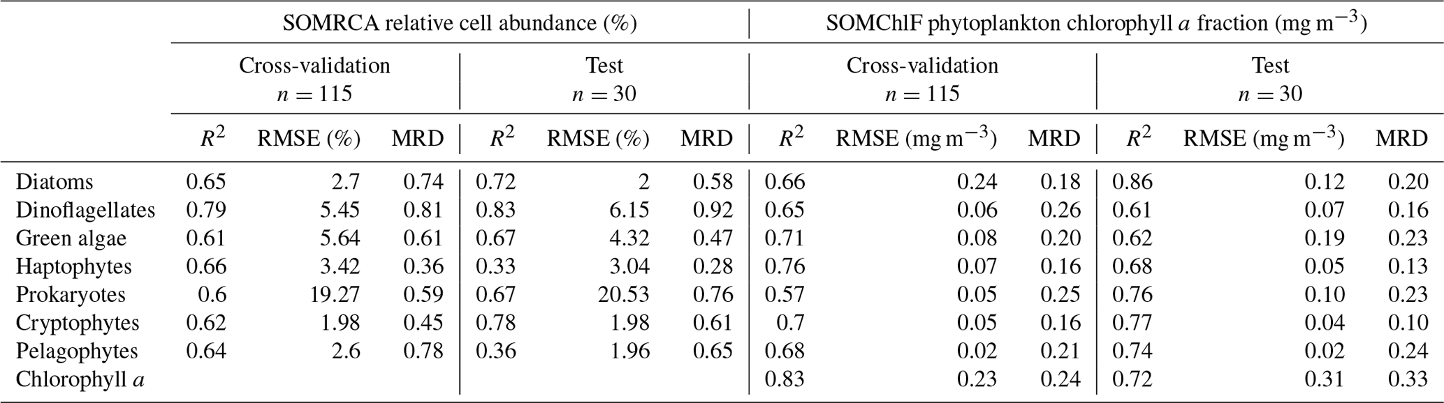
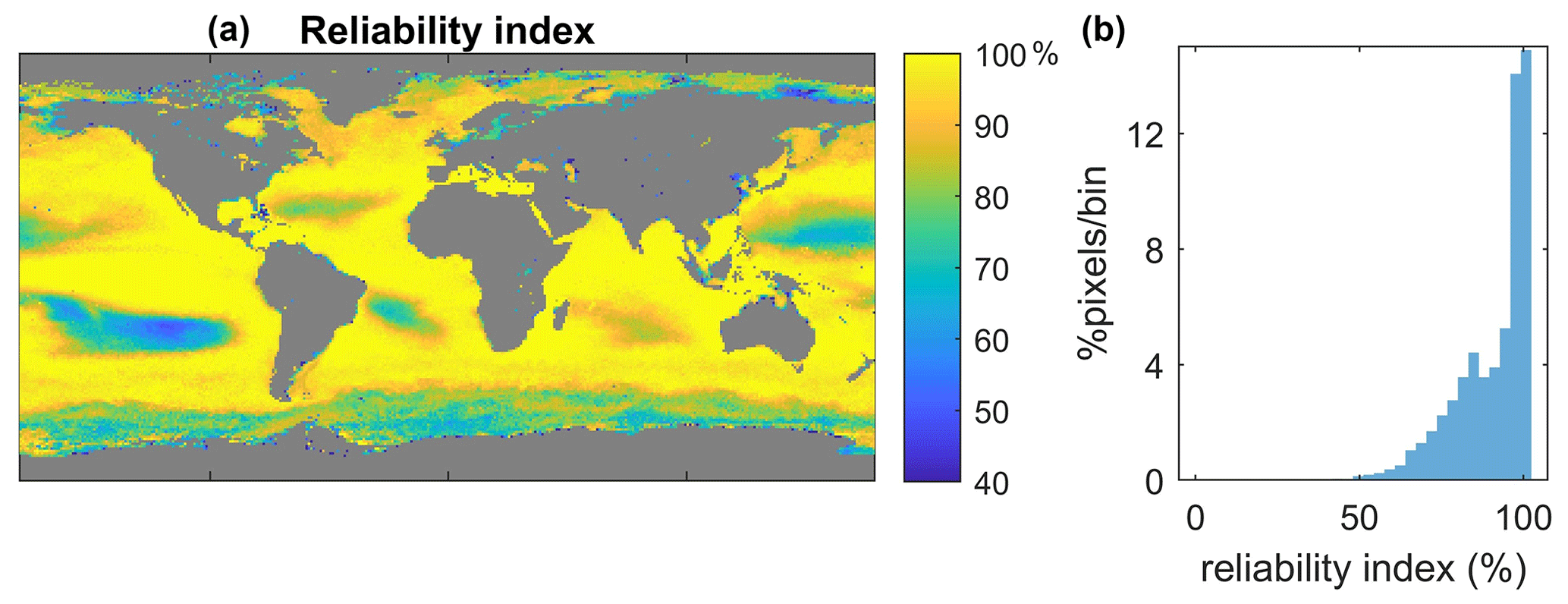
Figure 6Applicability of the satellite psbO-based method. The geographical (a) and value distributions (b) of the reliability index were calculated between 1997 and 2021 by testing the set of satellite parameters at a given pixel against the values in the original dataset (D).
4.2 Comparison with global HPLC pigment dataset
The global in situ HPLC dataset was then used to estimate Chl a fractions for each phytoplankton group using the diagnostic pigment approach (DPA). This dataset was compared to the Chl a fraction matching each phytoplankton group that was estimated by SOMChlF (Fig. 7). A total of 2671 matchups were found following the same procedure described in Sect. 3.1. Evaluating the sum of Chl a fractions and comparing it with in situ Chl a can be considered a baseline evaluation of this method. This comparison showed a satisfying correspondence score of R2=0.72. Relatively good correspondence is noted for diatoms and haptophytes, showing an R2=0.64 between in situ and SOMChlF for diatoms and 0.65 for haptophytes. Moderate correspondence was found for green algae, cryptophytes, and pelagophytes, with an R2 ranging between 0.43 and 0.39. Prokaryotes and dinoflagellates had the lowest correspondence between both outputs. The comparison between DPA-based phytoplankton groups and SOMChlF estimates is highly uncertain. It compares two types of information indicating the same phytoplankton group, with different underlying assumptions about how to define and describe a certain group. For some of the groups, these results are coherent. For example, the diatom Chl a fraction is well captured by the latter, and the values agree with those estimated using HPLC observations; however, we noted a major overestimation within the HPLC DPA method. For prokaryotes, this comparison leads us to say that using zeaxanthin as an indicator of the cyanobacterial contribution to Chl a may not entirely represent this group.
The permutation-based importance analysis using random forest, performed on the in situ Tara Oceans psbO and HPLC measurements, emphasizes the necessity of a multivariate approach for predicting phytoplankton community structure based on pigments (see Fig. 8). Notably, the diagnostic pigments mentioned in Table 1 exhibited dominant importance in determining the relative abundance of their respective assigned phytoplankton groups. For instance, peridinin represented dinoflagellates, chlorophyll b characterized green algae, and zeaxanthin indicated prokaryotes (Table 1). These pigments demonstrated the highest importance for their respective groups, as illustrated in Fig. 8, accompanied by a positive Spearman correlation. However, individually, these pigments accounted for less than 25 % of the variance in their respective groups. Conversely, in the case of cryptophytes, diatoms, and haptophytes, no pigment stood out in terms of importance, and the observed correlations were related to covariation between pigments (e.g., Chl b and Fuco in diatoms), possibly influenced by Chl a variability. Therefore, the variability within each group is best explained not by a single diagnostic pigment, but rather by the overall pigment composition. It is crucial to consider how natural variability can influence the interpretation of pigment composition in relation to phytoplankton community structure. Pigment ratios not only vary with phytoplankton composition but also reflect the diverse strategies employed by different phytoplankton types to acclimate to environmental factors such as light, temperature, nutrients, and other variables.
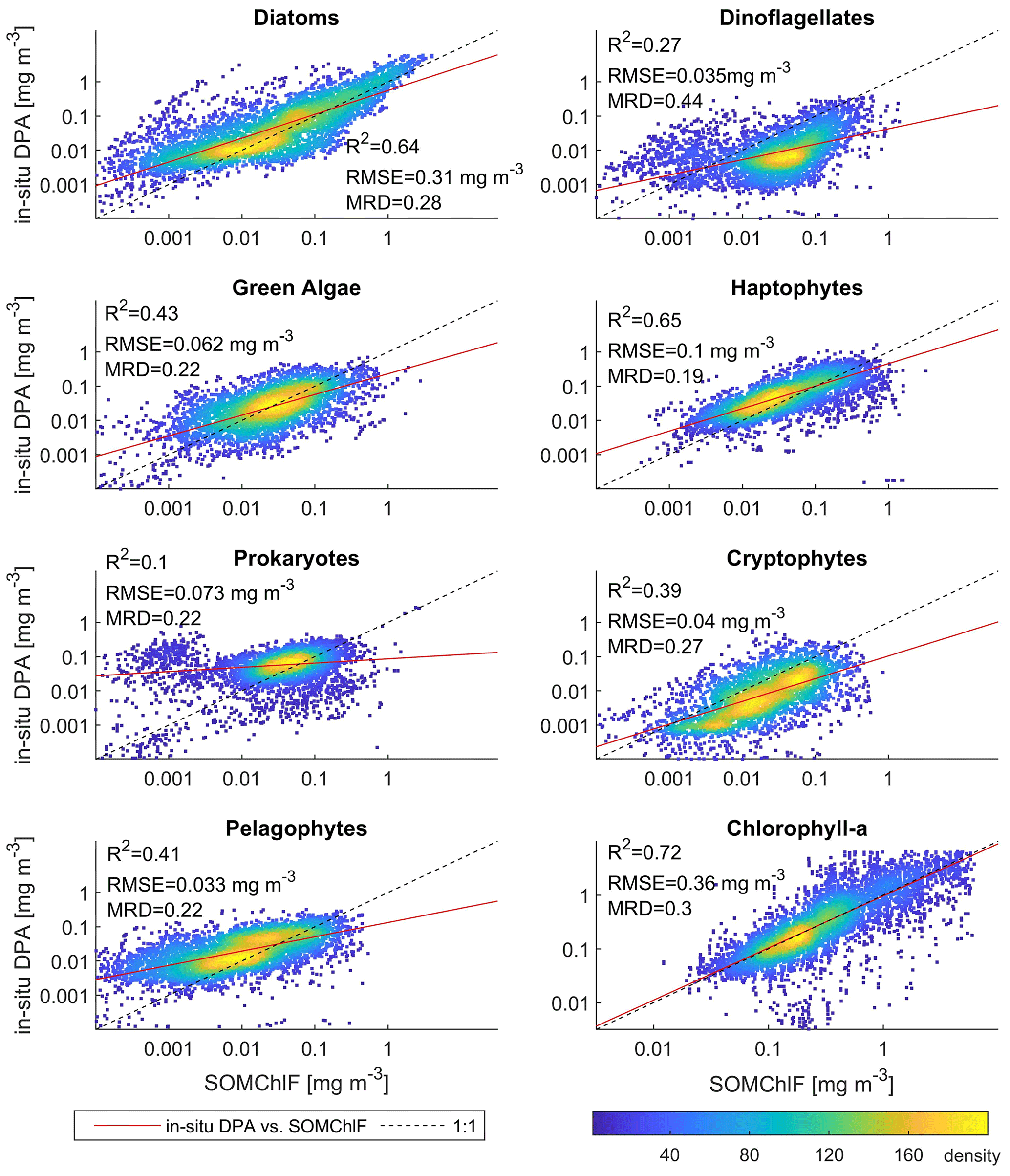
Figure 7Comparison between the outputs of SOMChlF and the DPA approach applied to an in situ global HPLC dataset. 2672 matchups were found between the outputs of SOMChlF and the in situ dataset and analyzed in this figure. The R2 and MRD result from calculations based on log-transformed data, and RMSE is based on non-log-transformed data.
4.3 Global patterns of satellite-derived phytoplankton groups
We then applied our method to GlobColour satellite data to generate a daily database spanning from 1997 to 2021, capturing the relative cell abundance and Chl a fraction of seven phytoplankton groups of interest. Figure 9 presents the annual patterns of relative cell abundance and Chl a fraction for each phytoplankton group, derived from this satellite dataset.
Regarding relative cell abundance, the prokaryotes stand out as a dominant group. This group largely dominated tropical regions, with a relative abundance of up to 80 % in subtropical gyres. Haptophytes, green algae, and diatoms exhibited higher abundance in middle and high latitudes as well as the equatorial region, showing a maximum relative abundance of 30 %. The remaining three phytoplankton groups displayed relative abundances that barely exceeded 10 % of the total phytoplankton community. Pelagophytes and dinoflagellates were primarily observed in middle and subtropical latitudes, while cryptophytes were found in coastal areas and high latitudes.
Examination of how each phytoplankton group contributed to total Chl a revealed that diatoms had a significant contribution at high latitudes and equatorial regions. Prokaryotes, on the other hand, had an overall low to moderate contribution to total Chl a.
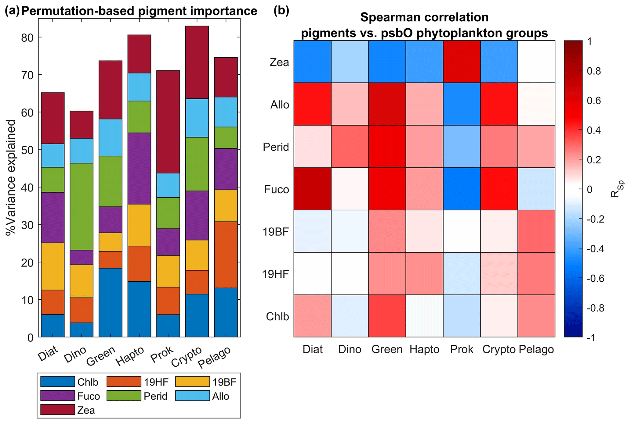
Figure 8Evaluation of secondary pigment weighting for the estimation of different phytoplankton groups. Panel (a) represents the percentage of variance of each phytoplankton group explained by a set of frequently used phytoplankton secondary pigments. This analysis has been done using a random forest algorithm applied to the in situ Tara Oceans psbO and HPLC datasets. A Spearman correlation coefficient has been calculated between each pigment and the phytoplankton groups (b).
Qualitatively, the information captured by SOMChlF was clustered into five groups, each characterized by a distinct remote sensing reflectance spectrum that corresponded to the phytoplankton community structure (Fig. 10). To illustrate the link between each group's contribution to total Chl a concentration and relative cell abundance, we depicted the latter while evaluating the pixel's assigned relative abundance values for each of the five clusters. This approach revealed that three out of the five clusters are dominated by prokaryotes in terms of cell abundance (C1, C2, and C3). However, based on their relative contribution to Chl a, C1 was found to be dominated by prokaryotes and dinoflagellates, C2 exhibited a mixed composition, and C3 and C4 represented diatoms and other eukaryotes, whereas C5 was predominantly composed of diatoms. The shift from relative cell abundance to size-integrated relative Chl a fraction illustrates how cell size influences Chl a contribution and variability.
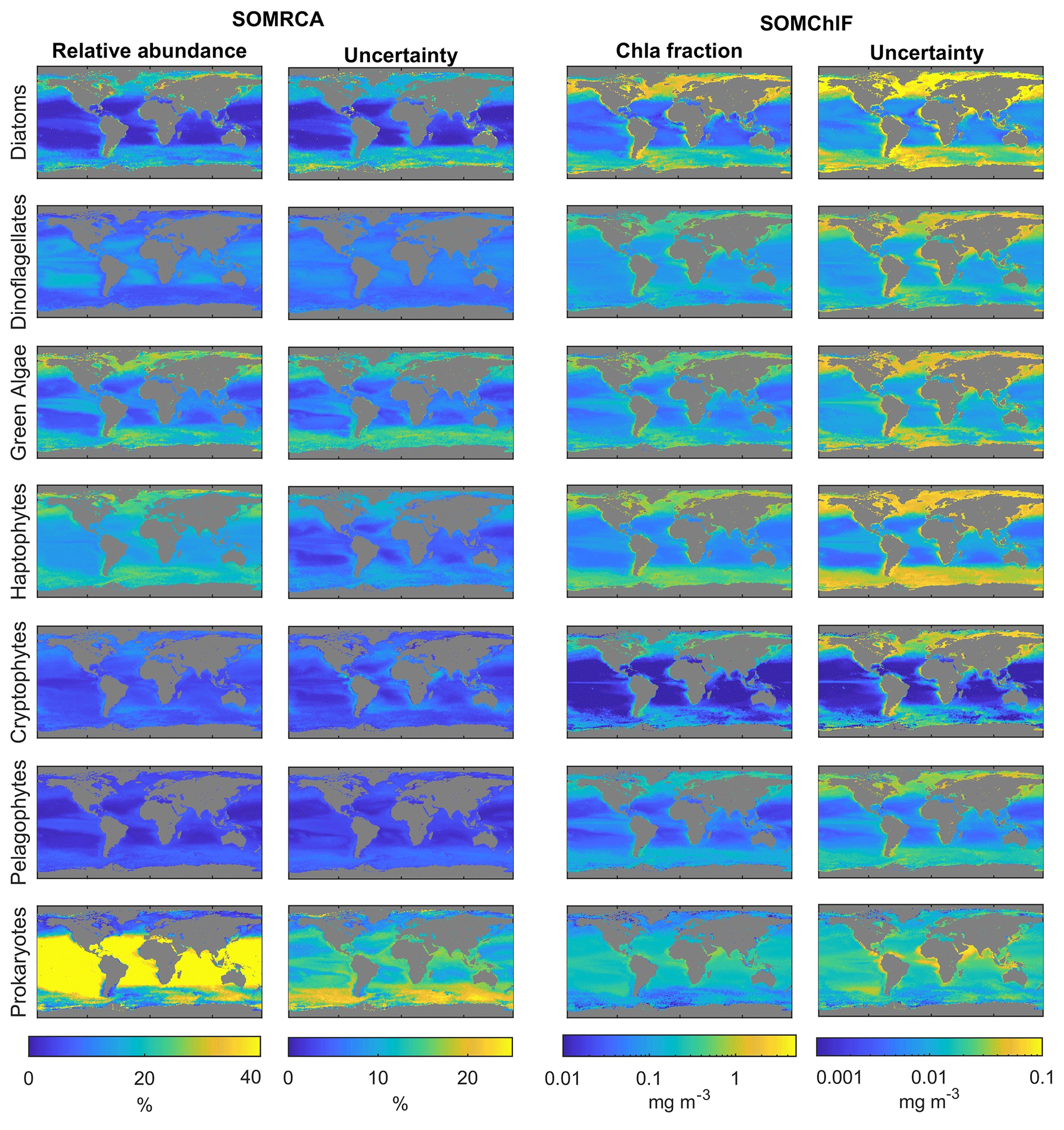
Figure 9Annual composites of the relative abundances and Chl fractions of the seven psbO-derived phytoplankton groups based on satellite data (compiled using data from 1997–2021). The uncertainties related to each group and each method are because of their different possible combinations through the weighted standard deviations, as described in Sect. 3.2.3. We note that the scales for uncertainty are smaller than those in the abundance and Chl a columns.
Each cluster is characterized by a specific optical signature in terms of Rrs spectra. The Rrs values per wavelength were normalized based on their corresponding variance, enabling intercomparison regardless of magnitude. For instance, C1, which exhibits higher reflectance in the blue wavelength, represents clear, oligotrophic waters. In such environments with low nutrients and high surface stratification, picophytoplankton groups like cyanobacteria thrive due to their high surface-to-size ratio (Raven, 1998; Chisholm, 1992). C2 represents normalized Rrs spectra with insignificant differences between normalized bands, suggesting an average state where the phytoplankton community appears mixed. In C3 and C4, we observed an increase in normalized Rrs values in the green compared to the blue wavebands, indicating higher Chl a in these environments. Given that C3 and C4 are located in high-latitude regions with ample nutrient resources and exceptional seasonal variability of light intensity, larger-cell-sized phytoplankton groups, including diatoms, are favored, leading to increased biomass and Chl a contribution (Brun et al., 2015). C5, with the greatest difference between Rrs in the blue and green, represents eutrophic waters, known for their high productivity and diatom-dominated blooms (Brun et al., 2015).
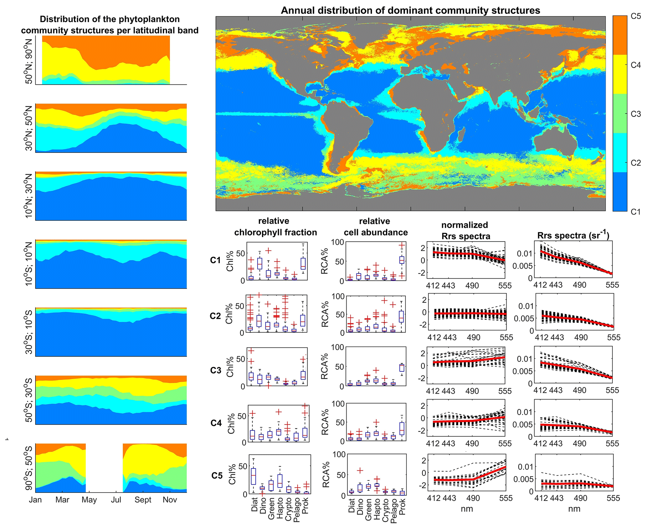
Figure 10Satellite-derived biomes of phytoplankton communities, obtained by unsupervised clustering (hierarchical clustering) of SOMChlF neurons. Relative cell abundances per phytoplankton group as well as normalized and denormalized Rrs spectra were also derived. The global map shows the most frequent community structure recorded during the 1997–2021 period. A spatiotemporal analysis was conducted to highlight latitudinal patterns.
Based on the global distributions of these clusters, several biomes can be defined. C1 is centered in subtropical gyres, C2 is found in transitional zones such as midlatitude regions and the equatorial region, C3 is observed in the Southern Ocean, C4 corresponds to high-latitude regions, and C5 is prevalent in coastal and eutrophic waters.
Different temporal variability is evident for each cluster across different latitudinal bands. In northern high latitudes, an increase in C5 indicates maximal productivity occurring in that region around May. At midlatitudes, the winter maximum is marked by an increase in C5 and C4 clusters. A secondary, less pronounced peak can be observed in autumn, attributed to the break in the thermocline and remineralization processes. During summer, C1 dominates the midlatitude regions. In tropical regions, C1 is predominant, with a cyclic increase in C2 suggesting coastal influences, likely due to the proximity of C2 to nutrient-rich zones like upwelling systems. In contrast to northern high latitudes, the Southern Ocean exhibits a different temporal variability. The presence of prokaryotes is signified by C1 in this region, whereas C3 dominates during the bloom season in January. This analysis confirms the Antarctic nature of C3 in contrast to C4, highlighting differences in water types between the two regions based on phytoplankton community structure and satellite data.
This division into parallel and transitional biomes underscores the significant influence of latitudinal physical gradients, including light availability and temperature, on the structuring of the phytoplankton community in terms of types and size. These findings align with previous global phytoplankton studies conducted in situ (Ibarbalz et al., 2019; Sommeria-Klein et al., 2021) as well as satellite estimates (Alvain et al., 2006; Hirata et al., 2011; Ben Mustapha et al., 2013; El Hourany et al., 2019a; Xi et al., 2020, 2021).
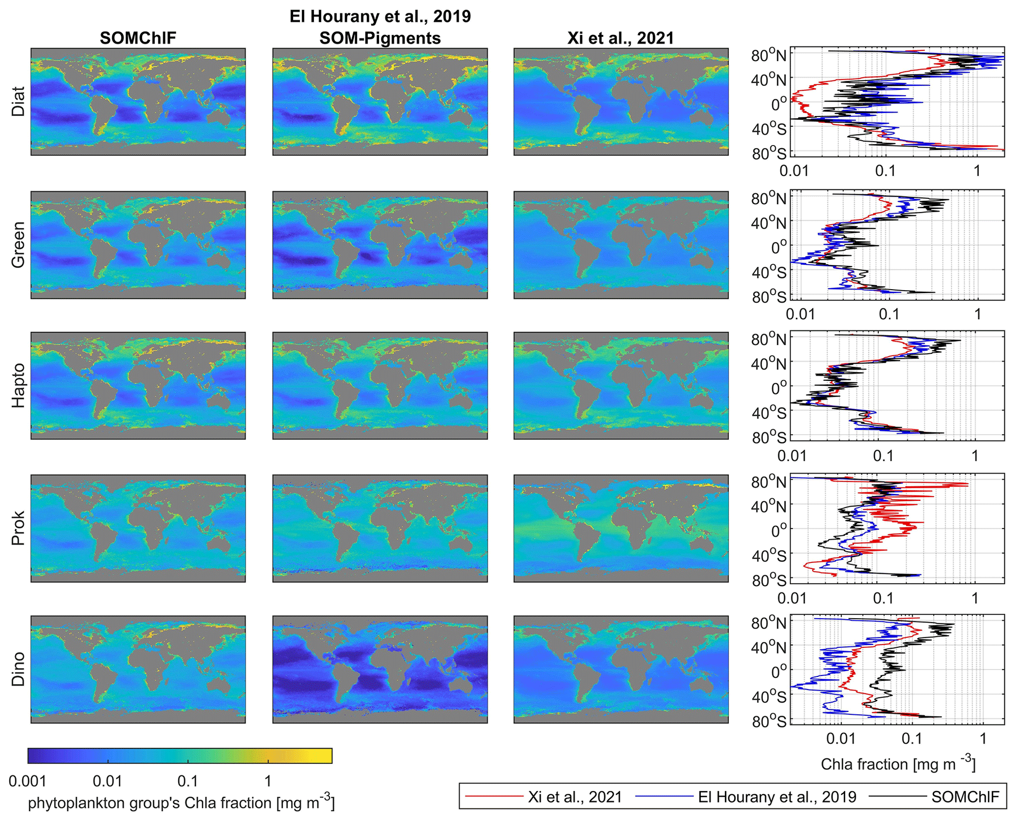
Figure 11Intercomparison of five satellite-derived phytoplankton group Chl a fractions based on the SOMChlF, SOM-Pigments (El Hourany et al., 2019a), and Xi et al. (2021) algorithms for the year 2020. The annual average and the average per latitude of each Chl a fraction are calculated to reveal global and latitudinal patterns.
4.4 Intercomparison of satellite-derived phytoplankton group products
A comparison was performed between SOMChlF output and two operational products based on the Xi et al. (2021) and SOM-Pigments (El Hourany et al., 2019a) algorithms. We based this on the five phytoplankton groups common to all three algorithms: diatoms, dinoflagellates, green algae, haptophytes, and prokaryotes for the year 2020. The annual patterns show substantial agreement between all three satellite-derived phytoplankton estimates (Fig. 11). However, some differences between the estimated quantities of Chl a phytoplankton groups can be noted. For diatoms, the outputs based on El Hourany et al. (2019a) and SOMChlF exhibit higher Chl a values, while those based on Xi et al. (2021) show low values near the equatorial latitudes. For green algae and haptophytes, the three products show matching latitudinal variability, with only minor discrepancies in values at high and subtropical latitudes. For prokaryotes, the outputs of Xi et al. (2021) show higher estimates, particularly near the Arctic and equatorial regions. Lastly, for dinoflagellates, the SOM-Pigments method yielded lower Chl a values, especially in subtropical gyres, whereas SOMChlF showed the highest Chl a estimates for this taxonomic group.
Upon comparing the uncertainty patterns with those observed in Xi et al. (2021), similar trends were identified for the Chl a fraction of eukaryotic phytoplankton, displaying consistency in following the Chl a concentration gradient as seen in our study. Notably, regions such as the gyres exhibited lower uncertainties, whereas higher uncertainties were evident in high-latitude regions and marginal seas. Conversely, when examining the uncertainty in the retrieval of prokaryote Chl a by Xi et al. (2021), lower uncertainties were noted in polar regions, contrasting with higher uncertainties observed in low-latitude regions. Similarly, in Brewin et al. (2017), the uncertainty maps for diatoms and dinoflagellates depicted distribution patterns akin to our uncertainty estimations in the North Atlantic Ocean.
This coherence in uncertainty patterns between HPLC-based products and our psbO-based product can be attributed to the direct relationship between DPA pigment concentration and total Chl a, as well as between psbO-derived Chl a fractions and total Chl a. Consequently, similar patterns in predictions, as well as in the uncertainties, emerge.
However, addressing the similarities and differences between the outputs of the above-cited methods referring to the same phytoplankton group is not a straightforward task. These methods are based on distinct assumptions and resolutions of phytoplankton groups; the estimation of phytoplankton groups using pigments is inherently imperfect and relies on assumptions that introduce considerable variability and bias in determining the contribution of specific pigments to the assessment of phytoplankton groups. For instance, several studies showed that the DPA approach tends to overestimate diatoms (Brewin et al., 2014; Chase et al., 2020). This approach may compromise the relevance of satellite images when used. However, the added value of such an approach resides in the availability of the large HPLC dataset, which allows the development of robust algorithms. On the other hand, the method described in this paper and the generated outputs are based for the first time on a complete and harmonized database of phytoplankton taxonomic community structure on a global scale, which is an approach that provides an unbiased picture of phytoplankton cell abundances. However, the major limitation of this approach at this time is the low number of observations from which the metric has been derived.
By employing an alternative approach utilizing in situ metagenomic observations, a reliable ocean color algorithm for detecting phytoplankton groups was developed in this work. This achievement is noteworthy considering the limited availability of omics data used in our analysis. The successful implementation was made possible by leveraging machine learning techniques and preserving the data structure using self-organizing maps. The methodology demonstrated satisfactory performance in producing robust estimates for the seven major phytoplankton groups, albeit with some limitations in terms of global generalization due to the limited availability of data. For instance, it is important to exercise caution when interpreting estimates for regions such as the subtropical gyres. As DNA sequencing costs continue to decrease and new expeditions generate molecular data from undersampled ocean regions, we expect the training datasets to increase rapidly in future years, which should further increase the accuracy of our method. Furthermore, this study presents a new global dataset of the relative cell abundances of the seven phytoplankton groups and their contributions to total Chl a. These two types of information carry different implications. Chl a serves as a biomass proxy, which is crucial for energy and matter fluxes in various ecological and biogeochemical processes. On the other hand, cell abundance represents species abundance for unicellular organisms, providing insights into community assembly processes.
This dataset opens up possibilities for intercomparisons with existing approaches, such as DPA-based methods using in situ and satellite data. The results provide coherent yet distinct information about phytoplankton communities, contributing to a better understanding of their composition. While our focus was on seven broad phytoplankton groups, it is worth mentioning that the deep taxonomic resolution achievable through molecular methods allows for species-level monitoring, which can be an interesting avenue for future implementation.
The methodology presented in this work provides a unique opportunity to observe the state of the major phytoplankton groups at the global scale in real time and at high resolution. This makes remote sensing observations excellent tools to collect EBVs, play the role of broker between monitoring initiatives and decision-makers, and provide a foundation for developing marine biodiversity forecasts under different policy and management scenarios. To reach this objective, remote sensing data inherently need to be validated with in situ observations as well. Of further interest is the launch of NASA's Plankton, Aerosol, Cloud, ocean Ecosystem (PACE) mission, a strategic climate continuity mission that will make global hyperspectral ocean color measurements possible. This will allow extended data records on ocean ecology and global biogeochemistry, revolutionizing the detection of phytoplankton communities from space. From the perspective of the PACE mission, this study is a step towards further understanding the effect of environmental changes on phytoplankton community structure and diversity.
| Acronym | Definition |
| PFT | Phytoplankton functional type |
| PG | Phytoplankton taxonomic group |
| PSC | Phytoplankton size class |
| HPLC | High-performance liquid chromatography |
| DPA | Diagnostic pigment analysis |
| DP | Diagnostic pigment |
| Chl a | Chlorophyll a |
| Fuco | Fucoxanthin |
| Perid | Peridinin |
| Allo | Alloxanthin |
| Zea | Zeaxanthin |
| Chlb | Chlorophyll b |
| 19HF | 19′-Hexanoyloxyfucoxanthin |
| 19BF | 19′-Butanoyloxyfucoxanthin |
| DVChl a | Divinyl-chlorophyll a |
| DVChl b | Divinyl-chlorophyll b |
| MAREDAT | MARine Ecosystem DATa |
| PSII | Photosystem II |
| OC | Ocean color |
| SeaWiFS | Sea-viewing Wide Field-of-view Sensor |
| MODIS | Moderate Resolution Imaging Spectroradiometer |
| VIIRS | Visible Infrared Imaging Radiometer Suite |
| MERIS | Medium Resolution Imaging Spectrometer |
| OLCI | Ocean and Land Colour Instrument |
| PACE | Plankton, Aerosol, Cloud, ocean Ecosystem mission |
| IOCCG | International Ocean Colour Coordinating Group |
| CCI | Climate Change Initiative |
| CMEMS | Copernicus Marine Environment Monitoring Service |
| Rrs | Remote sensing reflectance |
| Kd490 | Attenuation coefficient at 490 nm |
| PAR | Photosynthetically available radiation |
| NFLH | Normalized fluorescence line height |
| bbp | Particulate backscattering coefficient |
| SST | Sea surface temperature |
| SOM | Self-organizing map |
| AHC | Ascending hierarchical clustering |
| TD | Truncated distance |
| D | Initial dataset |
| DRCA | Phytoplankton groups' relative cell abundance sub-dataset to train SOMRCA |
| DChlF | Phytoplankton groups' chlorophyll a fraction per group sub-dataset to train SOMChlF |
| SOMRCA | SOM algorithm dedicated to estimating phytoplankton groups' relative cell abundance |
| SOMChlF | SOM algorithm dedicated to estimating phytoplankton groups' Chl a fraction |
| RMSE | Root mean squared error |
| R2 | Regression coefficient |
| MRD | Median relative deviation |
The psbO dataset can be found at https://www.ebi.ac.uk/biostudies/studies/S-BSST761 (Bowler and Pierella Karlusich, 2022). The GlobColour dataset can be found at https://hermes.acri.fr/index.php (ACRI-ST, 2019). The SST CCI dataset can be found at https://doi.org/10.48670/moi-00169 (ESA SST CCI and C3S reprocessed sea surface temperature analyses, 2019). The global HPLC pigment compiled dataset sources are MAREDAT (Peloquin et al., 2013), Polarstern data (Bracher, 2015a, b, c), Tara Oceans Expedition (Pesant et al., 2015), GeP&Co (Dandonneau et al., 2004), the NOMAD NASA Bio-Optical Marine Algorithm Dataset (Werdell and Bailey, 2005), and numerous campaigns found on the NASA SeaBASS portal (Werdell et al., 2003; Wright et al., 2010; de Salas et al., 2011). The MATLAB version of both operational SOM psbO algorithms, the training psbO, and satellite matchup dataset, along with the compiled HPLC data and their corresponding SOMChlF output matchups, can be accessed on Zenodo at the following links: https://doi.org/10.5281/zenodo.10361485 (El Hourany et al., 2024) and https://doi.org/10.5281/zenodo.10571578 (El Hourany, 2024). The MATLAB software library SOM Toolbox 2.1 was used, implementing the self-organizing map and hierarchical ascending classification algorithm © 1999 (by Esa Alhoniemi, Johan Himberg, Jukka Parviainen, and Juha Vesanto; accessible at https://github.com/ilarinieminen/SOM-Toolbox/tree/master, ilarinieminen, 2012). The MATLAB function for the random forest algorithm was used to run the algorithm (MATLAB version R2020b).
The supplement related to this article is available online at: https://doi.org/10.5194/os-20-217-2024-supplement.
Conceptualization: REH, ML, CB. Methodology: REH. Validation: REH, JPK. Formal analysis: REH, JPK, ML, CB. Investigation: REH, JPK, LZ, HL, ML, CB. Resources: ML, CB. Data curation: JPK, REH. Writing (original draft preparation): REH. Writing (review and editing): REH, JPK, LZ, HL, ML, CB. Visualization: REH. Supervision: ML, CB. Project administration: ML, CB. Funding acquisition: REH, ML, CB.
The contact author has declared that none of the authors has any competing interests.
Publisher's note: Copernicus Publications remains neutral with regard to jurisdictional claims made in the text, published maps, institutional affiliations, or any other geographical representation in this paper. While Copernicus Publications makes every effort to include appropriate place names, the final responsibility lies with the authors.
The authors acknowledge the recommendations and guidance of Emmanuel Boss (University of Maine) and Sylvie Thiria (Sorbonne University), as well as the constructive comments and suggestions provided by the editor and the four reviewers, which contributed to the enhancement of the paper. Roy El Hourany acknowledges CNES postdoc fellowship 2019–2021, ANR junior professor (ANR-22-CPJ1-0003-01), CNES TOSCA 2020–2021, Sorbonne University Emergence program 2021–2023, ML4BioChange, and IFSEA that benefits from grant ANR-21-EXES-0011. Juan Pierella Karlusich acknowledges postdoctoral funding from the Fonds Français pour l'Environnement Mondial. Chris Bowler acknowledges the ERC Advanced Award Diatomic (grant agreement no. 835067); the Horizon Europe projects AtlantECO (grant agreement no. 862923), Marco-Bolo (grant agreement no. 101082021), and BlueRemediomics (grant agreement no. 101082304); the French government “Investissements d'Avenir” programs OCEANOMICS (ANR-11-BTBR-0008), FRANCE GENOMIQUE (ANR-10-INBS-09-08), MEMO LIFE (ANR-10-LABX-54), and PSL Research University (ANR-11-IDEX-0001-02); and the BNP Paribas Foundation's Climate and Biodiversity Initiative. This article is contribution number 148 of Tara Oceans.
This research has been supported by the Centre National d'Etudes Spatiales (postdoctoral fellowship 2019–2021 and TOSCA BIODIV: Phytoplankton Diversity from Space), Sorbonne Université (ML4BioChange Emergence program 2021–2023), the European Research Council H2020 (diatomic project, grant agreement no. 835067), the Agence Nationale de la Recherche (CPJ – ANR-22-CPJ1-0003-01, Graduate school IFSEA – ANR-21-EXES-0011, OCEANOMICS – ANR-11-BTBR-0008, FRANCE GENOMIQUE – ANR-10-INBS-09-08, MEMO LIFE – ANR-10-LABX-54, and PSL Research University – ANR-11-IDEX-0001-02), the Fonds Français pour l'Environnement Mondial (postdoctoral fellowship), the ERC Advanced Award Diatomic (grant agreement no. 835067), AtlantECO (grant agreement no. 862923), the Horizon Europe projects Marco-Bolo (grant agreement no. 101082021) and BlueRemediomics (grant agreement no. 101082304), and the BNP Paribas Foundation's Climate and Biodiversity Initiative.
This paper was edited by Jochen Wollschlaeger and reviewed by Alison Chase and three anonymous referees.
ACRI-ST: The European Service for Ocean Colour – GlobColour, [data set], https://hermes.acri.fr/index.php (last access: 29 January 2024), 2019. a
Agustí, S.: Allometric Scaling of Light Absorption and Scattering by Phytoplankton Cells, Can. J. Fish. Aquat. Sci., 48, 763–767, https://doi.org/10.1139/f91-091, 1991. a
Alvain, S., Moulin, C., Dandonneau, Y., and Bréon, F.: Remote sensing of phytoplankton groups in case 1 waters from global SeaWiFS imagery, Deep-Sea Res. Pt. I, 52, 1989–2004, https://doi.org/10.1016/j.dsr.2005.06.015, 2005. a, b
Alvain, S., Moulin, C., Dandonneau, Y., Loisel, H., and Bréon, F. M.: A species-dependent bio-optical model of case I waters for global ocean color processing, Deep-Sea Res. Pt. I, 53, 917–925, https://doi.org/10.1016/j.dsr.2006.01.011, 2006. a
Ben Mustapha, Z., Alvain, S., Jamet, C., Loisel, H., and Dessailly, D.: Automatic classification of water-leaving radiance anomalies from global SeaWiFS imagery: Application to the detection of phytoplankton groups in open ocean waters, Remote Sens. Environ., 146, 97–112, https://doi.org/10.1016/j.rse.2013.08.046, 2013. a, b
Bock, N., Subramaniam, A., Juhl, A. R., Montoya, J., and Duhamel, S.: Quantifying per-cell chlorophyll a in natural picophytoplankton populations using fluorescence-activated cell sorting, Front. Mar. Sci., 9, 850646, https://doi.org/10.3389/fmars.2022.850646, 2022. a
Bowler, C. and Pierella Karlusich, J. J.: A robust approach to estimate relative phytoplankton cell abundances from metagenomes, BioStudies, S-BSST761, [data set], https://www.ebi.ac.uk/biostudies/studies/S-BSST761 (last access: 29 January 2024), 2022. a
Bracher, A., Taylor, M. H., Taylor, B., Dinter, T., Röttgers, R., and Steinmetz, F.: Using empirical orthogonal functions derived from remote-sensing reflectance for the prediction of phytoplankton pigment concentrations, Ocean Sci., 11, 139–158, https://doi.org/10.5194/os-11-139-2015, 2015a. a
Bracher, A., Taylor, M. H., Taylor, B., Dinter, T., Röttgers, R., and Steinmetz, F.: Using empirical orthogonal functions derived from remote-sensing reflectance for the prediction of phytoplankton pigment concentrations, Ocean Sci., 11, 139–158, https://doi.org/10.5194/os-11-139-2015, 2015b. a
Bracher, A., Taylor, M. H., Taylor, B., Dinter, T., Röttgers, R., and Steinmetz, F.: Using empirical orthogonal functions derived from remote-sensing reflectance for the prediction of phytoplankton pigment concentrations, Ocean Sci., 11, 139–158, https://doi.org/10.5194/os-11-139-2015, 2015c. a
Brewin, R. J., Sathyendranath, S., Jackson, T., Barlow, R., Brotas, V., Airs, R., and Lamont, T.: Influence of light in the mixed-layer on the parameters of a three-component model of phytoplankton size class, Remote Sens. Environ., 168, 437–450, https://doi.org/10.1016/J.RSE.2015.07.004, 2015. a, b, c, d, e
Brewin, R. J., Ciavatta, S., Sathyendranath, S., Jackson, T., Tilstone, G., Curran, K., Airs, R. L., Cummings, D., Brotas, V., Organelli, E., Dall'Olmo, G., and Raitsos, D. E.: Uncertainty in ocean-color estimates of chlorophyll for phytoplankton groups, Front. Mar. Sci., 4, 104, https://doi.org/10.3389/FMARS.2017.00104/BIBTEX, 2017. a
Brewin, R. J. W., Sathyendranath, S., Hirata, T., Lavender, S. J., Barciela, R. M., and Hardman-Mountford, N. J.: A three-component model of phytoplankton size class for the Atlantic Ocean, Ecol. Model., 221, 1472–1483, https://doi.org/10.1016/j.ecolmodel.2010.02.014, 2010. a
Brewin, R. J. W., Sathyendranath, S., Tilstone, G., Lange, P. K., and Platt, T.: A multicomponent model of phytoplankton size structure, J. Geophys. Res.-Oceans, 119, 3478–3496, https://doi.org/10.1002/2014JC009859, 2014. a
Brown, C.: Global Distribution of Coccolithophore Blooms, Oceanography, 8, 59–60, https://doi.org/10.5670/oceanog.1995.21, 1995. a
Brun, P., Vogt, M., Payne, M. R., Gruber, N., O'Brien, C. J., Buitenhuis, E. T., Le Quéré, C., Leblanc, K., and Luo, Y.-W.: Ecological niches of open ocean phytoplankton taxa, Limnol. Oceanogr., 60, 1020–1038, 2015. a, b
Charantonis, A. A., Testor, P., Mortier, L., D'Ortenzio, F., and Thiria, S.: Completion of a sparse GLIDER database using multi-iterative Self-Organizing Maps (ITCOMP SOM), Procedia Comput. Sci., 51, 2198–2206, 2015. a
Chase, A. P., Kramer, S. J., Haëntjens, N., Boss, E. S., Karp-Boss, L., Edmondson, M., and Graff, J. R.: Evaluation of diagnostic pigments to estimate phytoplankton size classes, Limnol. Oceanogr.-Meth., 18, 570–584, https://doi.org/10.1002/LOM3.10385, 2020. a, b
Chisholm, S. W.: Phytoplankton Size, in: Primary Productivity and Biogeochemical Cycles in the Sea, edited by: Falkowski, P. G., Woodhead, A. D., Vivirito, K., Environmental Science Research, vol 43. Springer, Boston, MA, https://doi.org/10.1007/978-1-4899-0762-2_12, 1962. a
da Silva, L. E. B. and Costa, J. A. F.: Clustering, noise reduction and visualization using features extracted from the self-organizing map, in: Intelligent Data Engineering and Automated Learning–IDEAL 2013: 14th International Conference, IDEAL 2013, Hefei, China, 20–23 October 2013, Proceedings 14, Springer, 242–251, 2013. a
Dairiki, C., Motokawa, S., Murata, A., and Taguchi, S.: How does cell volume influence the total light absorption efficiency of a mixed population of dinoflagellates with similar cell shapes and pigment compositions?, Plankton Benthos Res., 15, 250–258, 2020. a
Dandonneau, Y., Deschamps, P.-Y., Nicolas, J.-M., Loisel, H., Blanchot, J., Montel, Y., Thieuleux, F., and Bécu, G.: Seasonal and interannual variability of ocean color and composition of phytoplankton communities in the North Atlantic, equatorial Pacific and South Pacific, Deep-Sea Res. Pt. I, 51, 303–318, https://doi.org/10.1016/j.dsr2.2003.07.018, 2004. a
de Salas, M. F., Eriksen, R., Davidson, A. T., and Wright, S. W.: Protistan communities in the Australian sector of the Sub-Antarctic Zone during SAZ-Sense, Deep-Sea Res. Pt. II, 58, 2135–2149, 2011. a
Di Cicco, A., Sammartino, M., Marullo, S., and Santoleri, R.: Regional Empirical Algorithms for an Improved Identification of Phytoplankton Functional Types and Size Classes in the Mediterranean Sea Using Satellite Data, Front. Mar. Sci., 4, 126, https://doi.org/10.3389/fmars.2017.00126, 2017. a
Dutkiewicz, S., Cermeno, P., Jahn, O., Follows, M. J., Hickman, A. E., Taniguchi, D. A. A., and Ward, B. A.: Dimensions of marine phytoplankton diversity, Biogeosciences, 17, 609–634, https://doi.org/10.5194/bg-17-609-2020, 2020. a
El Hourany, R.: Satellite-derived phytoplankton community structure from space using psbO and machine learning, Zenodo [code], https://doi.org/10.5281/zenodo.10571578, 2024. a
El Hourany, R., Abboud-Abi Saab, M., Faour, G., Aumont, O., Crépon, M., and Thiria, S.: Estimation of secondary phytoplankton pigments from satellite observations using self-organizing maps (SOM), J. Geophys. Res.-Oceans, 124, 1357–1378, https://doi.org/10.1029/2018JC014450, 2019a. a, b, c, d, e, f, g, h, i
El Hourany, R., Abboud-Abi Saab, M., Faour, G., Mejia, C., Crépon, M., and Thiria, S.: Phytoplankton Diversity in the Mediterranean Sea From Satellite Data Using Self-Organizing Maps, J. Geophys. Res.-Oceans, 124, 5827–5843, https://doi.org/10.1029/2019JC015131, 2019b. a, b
El Hourany, R., Mejia, C., Faour, G., Crépon, M., and Thiria, S.: Evidencing the Impact of Climate Change on the Phytoplankton Community of the Mediterranean Sea Through a Bioregionalization Approach, J. Geophys. Res.-Oceans, 126, e2020JC016808, https://doi.org/10.1029/2020JC016808, 2021. a
El Hourany, R., Pierella Karlusich, J. J., Zinger, L., Loisel, H., Levy, M., and Bowler, C.: Linking satellites to genes with machine learning to estimate phytoplankton community structure from space, Zenodo [data set], https://doi.org/10.5281/zenodo.10361485, 2024. a
ESA SST CCI and C3S reprocessed sea surface temperature analyses: E.U. Copernicus Marine Service Information (CMEMS), Marine Data Store (MDS), [data set], https://doi.org/10.48670/moi-00169, 2019. a
Flombaum, P., Gallegos, J. L., Gordillo, R. A., Rincon, J., Zabala, L. L., Jiao, N., Karl, D. M., Li, W. K. W., Lomas, M. W., Veneziano, D., Vera, C. S., Vrugt, J. A., and Martiny, A. C.: Present and future global distributions of the marine Cyanobacteria Prochlorococcus and Synechococcus, P. Natl. Acad. Sci. USA, 110, 9824–9829, https://doi.org/10.1073/pnas.1307701110, 2013. a
Folguera, L., Zupan, J., Cicerone, D., and Magallanes, J. F.: Self-organizing maps for imputation of missing data in incomplete data matrices, Chemometr. Intell. Lab., 143, 146–151, 2015. a
Fuhrman, J. A.: Microbial community structure and its functional implications, 459, 193–199, https://doi.org/10.1038/nature08058, 2009. a
Fujiki, T. and Taguchi, S.: Variability in chlorophyll a specific absorption coefficient in marine phytoplankton as a function of cell size and irradiance, J. Plankton Res., 24, 859–874, 2002. a
Guidi, L., Stemmann, L., Jackson, G. A., Ibanez, F., Claustre, H., Legendre, L., Picheral, M., and Gorsky, G.: Effects of phytoplankton community on production, size, and export of large aggregates: A world-ocean analysis, Limnol. Oceanogr., 54, 1951–1963, https://doi.org/10.4319/LO.2009.54.6.1951, 2009. a
Henson, S. A., Cael, B. B., Allen, S. R., and Dutkiewicz, S.: Future phytoplankton diversity in a changing climate, Nat. Commun., 12, 1–8, https://doi.org/10.1038/s41467-021-25699-w, 2021. a
Hillebrand, H. and Azovsky, A. I.: Body size determines the strength of the latitudinal diversity gradient, Ecography, 24, 251–256, https://doi.org/10.1034/J.1600-0587.2001.240302.X, 2001. a
Hirata, T., Aiken, J., Hardman-Mountford, N., Smyth, T., and Barlow, R.: An absorption model to determine phytoplankton size classes from satellite ocean colour, Remote Sens. Environ., 112, 3153–3159, https://doi.org/10.1016/J.RSE.2008.03.011, 2008. a
Hirata, T., Hardman-Mountford, N. J., Brewin, R. J. W., Aiken, J., Barlow, R., Suzuki, K., Isada, T., Howell, E., Hashioka, T., Noguchi-Aita, M., and Yamanaka, Y.: Synoptic relationships between surface Chlorophyll-a and diagnostic pigments specific to phytoplankton functional types, Biogeosciences, 8, 311–327, https://doi.org/10.5194/bg-8-311-2011, 2011. a, b, c
Hood, R. R., Laws, E. A., Armstrong, R. A., Bates, N. R., Brown, C. W., Carlson, C. A., Chai, F., Doney, S. C., Falkowski, P. G., Feely, R. A., Friedrichs, M. A., Landry, M. R., Keith Moore, J., Nelson, D. M., Richardson, T. L., Salihoglu, B., Schartau, M., Toole, D. A., and Wiggert, J. D.: Pelagic functional group modeling: Progress, challenges and prospects, Deep-Sea Res. Pt. II, 53, 459–512, https://doi.org/10.1016/J.DSR2.2006.01.025, 2006. a
Ibarbalz, F. M., Henry, N., Brandão, M. C., Martini, S., Busseni, G., Byrne, H., Coelho, L. P., Endo, H., Gasol, J. M., Gregory, A. C., Mahé, F., Rigonato, J., Royo-Llonch, M., Salazar, G., Sanz-Sáez, I., Scalco, E., Soviadan, D., Zayed, A. A., Zingone, A., Labadie, K., Ferland, J., Marec, C., Kandels, S., Picheral, M., Dimier, C., Poulain, J., Pisarev, S., Carmichael, M., Pesant, S., Acinas, S. G., Babin, M., Bork, P., Boss, E., Bowler, C., Cochrane, G., de Vargas, C., Follows, M., Gorsky, G., Grimsley, N., Guidi, L., Hingamp, P., Iudicone, D., Jaillon, O., Karp-Boss, L., Karsenti, E., Not, F., Ogata, H., Poulton, N., Raes, J., Sardet, C., Speich, S., Stemmann, L., Sullivan, M. B., Sunagawa, S., Wincker, P., Pelletier, E., Bopp, L., Lombard, F., and Zinger, L.: Global Trends in Marine Plankton Diversity across Kingdoms of Life, Cell, 179, 1084–1097, https://doi.org/10.1016/J.CELL.2019.10.008, 2019. a, b
Iglesias-Rodríguez, M. D., Brown, C. W., Doney, S. C., Kleypas, J., Kolber, D., Kolber, Z., Hayes, P. K., and Falkowski, P. G.: Representing key phytoplankton functional groups in ocean carbon cycle models: Coccolithophorids, Global Biogeochem. Cy., 16, 1–20, https://doi.org/10.1029/2001GB001454, 2002. a
ilarinieminen: SOM Toolbox 2.1, [code], https://github.com/ilarinieminen/SOM-Toolbox/tree/master (last access: 29 January 2024), 2012. a
Irigoien, X., Hulsman, J., and Harris, R. P.: Global biodiversity patterns of marine phytoplankton and zooplankton, Nature, 429, 863–867, https://doi.org/10.1038/nature02593, 2004. a
Jouini, M., Lévy, M., Crépon, M., and Thiria, S.: Reconstruction of satellite chlorophyll images under heavy cloud coverage using a neural classification method, Remote Sens. Environ., 131, 232–246, https://doi.org/10.1016/j.rse.2012.11.025, 2013. a
Kaneko, H., Endo, H., Henry, N., Berney, C., Mahé, F., Poulain, J., Labadie, K., Beluche, O., El Hourany, R., et al.: Predicting global distributions of eukaryotic plankton communities from satellite data, ISME Commun., 3, 101, https://doi.org/10.1038/s43705-023-00308-7, 2023. a
Le Quéré, C., Harrison, S. P., Colin Prentice, I., Buitenhuis, E. T., Aumont, O., Bopp, L., Claustre, H., Cotrim Da Cunha, L., Geider, R., Giraud, X., Klaas, C., Kohfeld, K. E., Legendre, L., Manizza, M., Platt, T., Rivkin, R. B., Sathyendranath, S., Uitz, J., Watson, A. J., and Wolf-Gladrow, D.: Ecosystem dynamics based on plankton functional types for global ocean biogeochemistry models, Global Change Biol., 11, 2016–2040, https://doi.org/10.1111/j.1365-2486.2005.1004.x, 2005. a
Losa, S. N., Soppa, M. A., Dinter, T., Wolanin, A., Brewin, R. J., Bricaud, A., Oelker, J., Peeken, I., Gentili, B., Rozanov, V., et al.: Synergistic exploitation of hyper-and multi-spectral precursor sentinel measurements to determine phytoplankton functional types (SynSenPFT), Front. Mar. Sci., 4, 203, https://doi.org/10.3389/fmars.2017.00203, 2017. a, b
Mitchell, B. G., Brody, E. A., Holm-Hansen, O., McClain, C., and Bishop, J.: Light limitation of phytoplankton biomass and macronutrient utilization in the Southern Ocean, Limnol. Oceanogr., 36, 1662–1677, https://doi.org/10.4319/lo.1991.36.8.1662, 1991. a
O'Reilly, J. E., Maritorena, S., Mitchell, B. G., Siegel, D. a., Carder, K. L., Garver, S. a., Kahru, M., and McClain, C.: Ocean color chlorophyll algorithms for SeaWiFS, J. Geophys. Res., 103, 24937, https://doi.org/10.1029/98JC02160, 1998. a
Organelli, E., Bricaud, A., Antoine, D., and Uitz, J.: Multivariate approach for the retrieval of phytoplankton size structure from measured light absorption spectra in the Mediterranean Sea (BOUSSOLE site), Appl. Opt., 52, 2257, https://doi.org/10.1364/AO.52.002257, 2013. a
Peloquin, J., Swan, C., Gruber, N., Vogt, M., Claustre, H., Ras, J., Uitz, J., Barlow, R., Behrenfeld, M., Bidigare, R., Dierssen, H., Ditullio, G., Fernandez, E., Gallienne, C., Gibb, S., Goericke, R., Harding, L., Head, E., Holligan, P., Hooker, S., Karl, D., Landry, M., Letelier, R., Llewellyn, C. A., Lomas, M., Lucas, M., Mannino, A., Marty, J.-C., Mitchell, B. G., Muller-Karger, F., Nelson, N., O'Brien, C., Prezelin, B., Repeta, D., Jr. Smith, W. O., Smythe-Wright, D., Stumpf, R., Subramaniam, A., Suzuki, K., Trees, C., Vernet, M., Wasmund, N., and Wright, S.: The MAREDAT global database of high performance liquid chromatography marine pigment measurements, Earth Syst. Sci. Data, 5, 109–123, https://doi.org/10.5194/essd-5-109-2013, 2013. a
Pereira, H. M., Ferrier, S., Walters, M., Geller, G. N., Jongman, R. H., Scholes, R. J., Bruford, M. W., Brummitt, N., Butchart, S. H., Cardoso, A. C., Coops, N. C., Dulloo, E., Faith, D. P., Freyhof, J., Gregory, R. D., Heip, C., Höft, R., Hurtt, G., Jetz, W., Karp, D. S., McGeoch, M. A., Obura, D., Onoda, Y., Pettorelli, N., Reyers, B., Sayre, R., Scharlemann, J. P., Stuart, S. N., Turak, E., Walpole, M., and Wegmann, M.: Essential biodiversity variables, Science, 339, 277–278, 2013. a
Pesant, S., Not, F., Picheral, M., Kandels-Lewis, S., Le Bescot, N., Gorsky, G., Iudicone, D., Karsenti, E., Speich, S., Trouble, R., Dimier, C., and Searson, S.: Open science resources for the discovery and analysis of Tara Oceans data, Sci. Data, 2, 1–16, https://doi.org/10.1038/SDATA.2015.23, 2015. a
Pierella Karlusich, J. J., Ibarbalz, F. M., and Bowler, C.: Phytoplankton in the Tara Ocean, Annu. Rev. Mar. Sci., 12, 233–265, https://doi.org/10.1146/ANNUREV-MARINE-010419-010706, 2020. a, b
Pierella Karlusich, J. J., Pelletier, E., Zinger, L., Lombard, F., Zingone, A., Colin, S., Gasol, J. M., Dorrell, R. G., Henry, N., Scalco, E., Acinas, S. G., Wincker, P., de Vargas, C., and Bowler, C.: A robust approach to estimate relative phytoplankton cell abundances from metagenomes, Molec. Ecol. Resour., 23, 16–40, https://doi.org/10.1111/1755-0998.13592, 2022. a, b, c
Powell, M. G. and Glazier, D. S.: Asymmetric geographic range expansion explains the latitudinal diversity gradients of four major taxa of marine plankton, Paleobiology, 43, 196–208, https://doi.org/10.1017/PAB.2016.38, 2017. a
Raven, J.: The twelfth Tansley Lecture. Small is beautiful: the picophytoplankton, Funct. Ecol., 12, 503–513, 1998. a
Rejeb, S., Duveau, C., and Rebafka, T.: Self-organizing maps for exploration of partially observed data and imputation of missing values, Chemometr. Intell. Lab., 231, 104653, https://doi.org/10.1016/j.chemolab.2022.104653, 2022. a
Reygondeau, G., Irisson, J.-O., Ayata, S. D., Gasparini, S., Benedetti, F., Albouy, C., Hattab, T., Guieu, C., and Koubbi, P.: Definition of the Mediterranean Eco-regions and Maps of Potential Pressures in These Eco-regions, Tech. Rep., Perseus Deliverable 1, http://www.perseus-net.eu/assets/media/PDF/deliverables/3336.6_Final.pdf (last access: 26 Janaury 2024), 2014. a
Richardson, A. J., Risien, C., and Shillington, F. A.: Using self-organizing maps to identify patterns in satellite imagery, Prog. Oceanogr., 59, 223–239, https://doi.org/10.1016/j.pocean.2003.07.006, 2003. a
Righetti, D., Vogt, M., Gruber, N., Psomas, A., and Zimmermann, N. E.: Global pattern of phytoplankton diversity driven by temperature and environmental variability, Sci. Adv., 5, 6253–6268, 2019. a
Rodríguez-Ramos, T., Marañón, E., and Cermeño, P.: Marine nano- and microphytoplankton diversity: redrawing global patterns from sampling-standardized data, Global Ecol. Biogeogr., 24, 527–538, https://doi.org/10.1111/GEB.12274, 2015. a
Rossi, V., Ser-Giacomi, E., Lõpez, C., and Hernández-García, E.: Hydrodynamic provinces and oceanic connectivity from a transport network help designing marine reserves, Geophys. Res. Lett., 41, 2883–2891, https://doi.org/10.1002/2014GL059540, 2014. a
Saitoh, F.: An ensemble model of self-organizing maps for imputation of missing values, in: 2016 IEEE 9th International Workshop on Computational Intelligence and Applications (IWCIA), 9–14, https://doi.org/10.1109/IWCIA.2016.7805741, 2016. a
Sarzeaud, O. and Stephan, Y.: Data interpolation using Kohonen networks, Proceedings of the International Joint Conference on Neural Networks, 6, 197–202, 2000. a
Sathyendranath, S., Aiken, J., Alvain, S., Barlow, R., Bouman, H., Bracher, A., Brewin, R., Bricaud, A., Brown, C. W., Ciotti, A. M., Clementson, L. A., Craig, S. E., Devred, E., Hardman-Mountford, N., Hirata, T., Hu, C., Kostadinov, T. S., Lavender, S., Loisel, H., Moore, T. S., Morales, J., Mouw, C. B., Nair, A., Raitsos, D., Roesler, C., Shutler, J. D., Sosik, H. M., Soto, I., Stuart, V., Subramaniam, A., and Uitz, J.: Phytoplankton functional types from Space, International Ocean-Colour Coordinating Group, Dartmouth, Nova Scotia, B2Y 4A2, Canada, ioccg; 15 Edn., https://epic.awi.de/id/eprint/36000/ (last access: 26 Janaury 2024), 2014. a
Sawadogo, S., Brajard, J., Niang, A., Lathuiliere, C., Crepon, M., and Thiria, S.: Analysis of the Senegalo-Mauritanian upwelling by processing satellite remote sensing observations with topological maps, 2009 International Joint Conference on Neural Networks, Atlanta, GA, USA, 28260–2832, https://doi.org/10.1109/IJCNN.2009.5178623, 2009. a
Smith, V. H.: Microbial diversity–productivity relationships in aquatic ecosystems, FEMS Microb. Ecol., 62, 181–186, https://doi.org/10.1111/J.1574-6941.2007.00381.X, 2007. a
Sommeria-Klein, G., Watteaux, R., Ibarbalz, F. M., Karlusich, J. J. P., Iudicone, D., Bowler, C., and Morlon, H.: Global drivers of eukaryotic plankton biogeography in the sunlit ocean, Science, 374, 594–599, 2021. a, b
Soppa, M. A., Hirata, T., Silva, B., Dinter, T., Peeken, I., Wiegmann, S., and Bracher, A.: Global retrieval of diatom abundance based on phytoplankton pigments and satellite data, Remote Sens., 6, 10089–10106, https://doi.org/10.3390/rs61010089, 2014. a, b, c, d
Tara Ocean Foundation: Tara Oceans, European Molecular Biology Laboratory (EMBL), Priorities for ocean microbiome research, Nat. Microbiol., 7, 937–947, https://doi.org/10.1038/s41564-022-01145-5, 2022. a
Taylor, B. B., Torrecilla, E., Bernhardt, A., Taylor, M. H., Peeken, I., Röttgers, R., Piera, J., and Bracher, A.: Bio-optical provinces in the eastern Atlantic Ocean and their biogeographical relevance, Biogeosciences, 8, 3609–3629, https://doi.org/10.5194/bg-8-3609-2011, 2011. a
Tilman, D., Isbell, F., and Cowles, J. M.: Biodiversity and Ecosystem Functioning, Annu. Rev. Ecol. Evol. Syst, 45, 471–493, https://doi.org/10.1146/annurev-ecolsys-120213-091917, 2014. a
Torrecilla, E., Stramski, D., Reynolds, R. A., Millán-Núñez, E., and Piera, J.: Cluster analysis of hyperspectral optical data for discriminating phytoplankton pigment assemblages in the open ocean, Remote Sens. Environ., 115, 2578–2593, 2011. a
Uitz, J., Claustre, H., Morel, A., and Hooker, S. B.: Vertical distribution of phytoplankton communities in open ocean: An assessment based on surface chlorophyll, J. Geophys. Res., 111, C08005, https://doi.org/10.1029/2005jc003207, 2006. a, b, c, d, e
Vidussi, F., Claustre, H., Manca, B. B., Luchetta, A., and Marty, J.-C.: Phytoplankton pigment distribution in relation to upper thermocline circulation in the eastern Mediterranean Sea during winter, J. Geophys. Res.-Oceans, 106, 19939–19956, https://doi.org/10.1029/1999JC000308, 2001. a
Werdell, P. J. and Bailey, S. W.: An improved in-situ bio-optical data set for ocean color algorithm development and satellite data product validation, Remote Sens. Environ., 98, 122–140, https://doi.org/10.1016/j.rse.2005.07.001, 2005. a
Werdell, P. J., Bailey, S., Fargion, G., Pietras, C., Knobelspiesse, K., Feldman, G., and McClain, C.: Unique data repository facilitates ocean color satellite validation, Eos, 84, 377–387, 2003. a
Wright, S. W., van den Enden, R. L., Pearce, I., Davidson, A. T., Scott, F. J., and Westwood, K. J.: Phytoplankton community structure and stocks in the Southern Ocean (30–80∘ E) determined by CHEMTAX analysis of HPLC pigment signatures, Deep-Sea Res. Pt. II, 57, 758–778, 2010. a
Xi, H., Losa, S. N., Mangin, A., Soppa, M. A., Garnesson, P., Demaria, J., Liu, Y., D'Andon, O. H. F., and Bracher, A.: Global retrieval of phytoplankton functional types based on empirical orthogonal functions using CMEMS GlobColour merged products and further extension to OLCI data, Remote Sens. Environ., 240, 111704, https://doi.org/10.1016/J.RSE.2020.111704, 2020. a, b
Xi, H., Losa, S. N., Mangin, A., Garnesson, P., Bretagnon, M., Demaria, J., Soppa, M. A., Hembise Fanton d'Andon, O., and Bracher, A.: Global chlorophyll a concentrations of phytoplankton functional types with detailed uncertainty assessment using multisensor ocean color and sea surface temperature satellite products, J. Geophys. Res.-Oceans, 126, e2020JC017127, https://doi.org/10.1029/2020JC017127, 2021. a, b, c, d, e, f, g, h, i