Study of the role of abyssal ocean stratification in the rearrangement of potential vorticity through the water column

Observations of abyssal variability performed in the Ionian Sea (Mediterranean Sea) have revealed the presence of a dense, stable abyssal layer, whose thermohaline and dynamical properties changed drastically over a decade. Building upon these available observations, we aim to investigate the role that stratification can play in the transmission of vorticity throughout the water column to the abyss and, in turn, in the redistribution of energy stored in the deep sea, with a set of stationary states. A quasi-geostrophic level model equipped with four coupled layers, a free surface, and a mathematical artifice for parameterizing decadal time evolution has been considered, proving that the relative-thickness and relative-density differences among the layers are the two critical factors that determine the dynamical characteristics of this rearrangement. The variability in ocean stratification is a relevant aspect that can activate deep and intermediate dynamics, engaging in the propagation and stabilization of signals throughout the water column. This demonstrates the non-negligible active connection between the dynamics of the bottom layers and the surface. The theoretical framework and parameterization used are based on specific observations made in the Ionian Sea over the last decades but retain general applicability to all ocean basins that are characterized by the presence of a stratified, dense water mass in their deep and intermediate layers.

1 Introduction

The effects of deep variability on dynamics at the surface and intermediate depths are generally not well investigated, despite growing evidence of the large amount of thermal energy stored in the abyss (Desbruyères et al., 2016; Riser et al., 2016; Meyssignac et al., 2019; Johnson and Doney, 2006; Heuzé et al., 2022). The role of deep dynamics in redistributing this energy through small-scale mixing activation is far from negligible, yet it remains an open question (Ferrari et al., 2016; De Lavergne et al., 2016; Mashayek et al., 2017b, a; McDougall and Ferrari, 2017).

Given the dynamical characteristics of the Mediterranean Sea, which is generally considered a “miniature ocean” as its thermohaline circulation is governed by density-driven processes (Bethoux et al., 1999), this sea serves as an ideal laboratory for investigating the impact of stratification on abyssal processes as it exhibits shorter timescales than those associated with the global oceans. In particular, the Ionian Sea, located in the eastern part of the Mediterranean Sea, is a perfect site for studying abyssal dynamics because it connects two main areas of deep-water formation (i.e., the Adriatic and Aegean seas), and its deep variability is particularly interesting with regard to ocean circulation (Theocharis et al., 1993; Pinardi et al., 2019; Wüst, 1961; Hainbucher et al., 2006; Malanotte-Rizzoli et al., 1999). This makes the Ionian Sea representative of ocean basins with deep- and intermediate-water inputs, giving this case study broader applicability.

Observations made in the depths of the Ionian Sea over the last 30 years or more – based on deep-profiling CTD (conductivity–temperature–depth) casts, moorings, and seafloor observatories – reveal variability at both interannual and decadal scales, thus showing how active the Mediterranean abyss is (Artale et al., 2018; Hainbucher et al., 2006; Manca et al., 2006; Budillon et al., 2010), despite the sparse observations and the time series gaps. The dense and stable stratification of the deep layer of the Ionian Sea, observed in nearly full-depth profiles, could be a key condition for observing deep variability (Giambenedetti et al., 2023). Analysis of different datasets on the deep layers of the Ionian Sea suggests the presence of vorticity, likely generated by stream instability in the deep layers (Rubino et al., 2012; Giambenedetti et al., 2023). Despite advancements in technology, the scarcity of available data obtained below 2000 m of depth remains a challenge that limits our understanding of the deep sea. To address this gap and gain deeper insights into this complex system, it is crucial to integrate approaches combining existing observations, theories, and numerical models.

To investigate the role that stratification can play in the transmission of perturbations at depth, we started with hydrological observations of the Ionian Sea. The observed structure suggests that a four-layer scheme should provide a realistic yet straightforward theoretical representation. This representation adds some complexity to the general view of the Ionian Sea as a two-layer system (Rubino et al., 2020; Gačić et al., 2021).

Since we want to focus on the abyss response rather than the more active surface and intermediate layers, the quasi-geostrophic (QG) approximation theory is most suitable for addressing our problem. Hence, we focused on potential vorticity, which can be induced by circulation and gyres and whose dynamic variability is known to control flow stability in rotating fluids (Sutyrin, 2015; Dritschel, 1989). The stability of vortices is indeed considered an important topic as it plays an active role in the redistribution of excess heat in the ocean (Wunsch and Ferrari, 2004; Cushman-Roisin, 1987; Armi, 1978; Cessi et al., 2006; Danabasoglu et al., 1994; Abernathey et al., 2010). However, many vortices in nature have a longevity that is not correctly represented by theory (Benilov, 2005; Rubino et al., 2007). One proposed explanation for this longevity is the stabilizing effect of bottom topography, as noted by Gulliver and Radko (2022), which is an important effect that is often neglected. As suggested by Giambenedetti et al. (2023), the presence of stable deep stratification can enhance topographic effects. Particularly when considering abyssal dynamics, focusing on topography alone leaves open questions about the connection between different layers throughout the water column.

Typically, potential-vorticity studies focus on surface and intermediate layers, which have more rapid responses compared to abyssal layers and are characterized by many energetic processes, such as thermocline ventilation and diabatic mixing (Smith and Vallis, 2001; Yassin and Griffies, 2022).

Given the presence of the dense abyssal layer observed in the Ionian Sea, the best representation is provided by a QG equation with four nonlinearly coupled levels, with parameters based on in situ data. We used a level model instead of a layer model, meaning the discretization uses a vertical z coordinate instead of a ρ coordinate to follow isopycnals. The two schemes are equivalent when ρ is considered a linear function of z, but this is not the case here. In fact, the density structure observed in the Ionian Sea abyss is not linear with depth; hence, we needed a coordinate that accounts for this variability throughout the entire water column. In numerical models of the ocean, both approaches are combined: the vertical coordinate is typically used only in surface layers, while the interior, which is considered more stable, is treated using isopycnals (Griffies et al., 2000).

The presence of significant relative-density differences in abyssal layers represents not only a local phenomenon in the Ionian Sea, but also a wider trend in the global oceans as ocean stratification has increased substantially over the past decades, even at great depths (Izquierdo and Mikolajewicz, 2019; Heuzé et al., 2022). Hence, our study also aims to highlight that abyssal stratification should receive more attention in models as neglecting its presence could lead to biased representations of ocean dynamics.

The approach used is the “equivalent barotropic” method, which is the simplest way to realistically account for the effects of stratification (Benzi et al., 1982). To further simplify the model, no external forcing is applied, bathymetry is ignored, and only dissipation is retained. Moreover, a small-scale dissipation term and a numerical damping term are included in the solution of the QG equation system to stabilize noise.

Each stratification configuration is solved over time to reach stability, assumed as the state where dissipation between consecutive iterations becomes negligible, resulting in a set of stationary states. This can be seen as a time parameterization, meaning that the different thicknesses of the deep layers can be representative of the stratification structures evolving over decades, which reflects the timescales of the deep-stratification adjustment observed during the Eastern Mediterranean Transient (EMT) in the Ionian Sea (Artale et al., 2018; Klein et al., 1999; Malanotte-Rizzoli et al., 1999). The EMT consisted of a transition of deep Ionian water sources from the Adriatic Sea to the Aegean Sea, which is warmer and saltier, leading to a drastic change in stratification and affecting Mediterranean Sea circulation over the following decades. This event, which started in the early 1990s, stimulated intense research, but the causes are still debated within the oceanographic community. The EMT has generally been linked to surface changes (Borzelli et al., 2009; Pinardi et al., 2019; Amitai et al., 2017) impacting the deep layers, without considering the reverse process or the concurrence of deep and surface mechanisms in the process.

The mathematical artifice we decided to implement to parameterize the different timescales involved in abyssal-stratification changes provides a way of looking at the complexity of the connection between surface and depth from an upside-down point of view, with the aim of explaining the observed variability in the Ionian abyssal layers.

2 Observations and problem formulation

In Giambenedetti et al. (2023), the presence of a deep, dense, stable layer in the Ionian Sea is shown, along with an enhancement of diffusivity in the abyssal layer due to tides. The presence of this stable layer has been suggested as a key means of observing mixing activation in the abyss. The dataset presented in Giambenedetti et al. (2023) has been integrated here with long time series of CTD and current meter data from the multidisciplinary seafloor observatory NEMO-SN1.

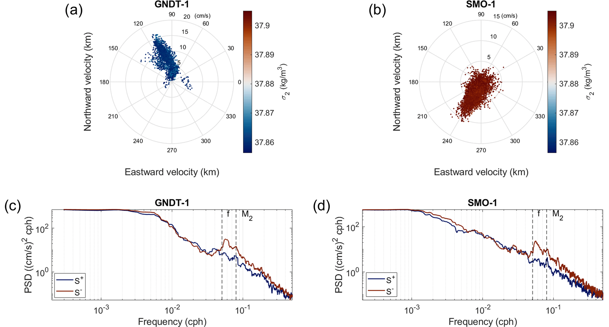
Figure 1 Current hodographs for the (a) 2002–2003 (GNDT 1) and (b) 2012–2013 (SMO 1) NEMO-SN1 missions, with the color bars indicating density anomaly (σ₂) values (Lilly and Rhines, 2002). Rotary spectra for the (c) 2002–2003 (GNDT 1) and (d) 2012–2013 (SMO 1) current meter data from NEMO-SN1, where different colors represent clockwise/anticlockwise spectra (S±). The dashed gray lines indicate the inertial (f) and tidal (M₂) frequencies. PSD: power spectral density.

NEMO-SN1 is located in the western Ionian Sea off eastern Sicily (Italy), about 25 km from the coast (37.5° N, 15.4° E), at a depth of 2100 m, and the two missions referred to in this study were carried out from October 2002 to February 2003 (GNDT 1) and from June 2012 to June 2013 (SMO 1) (Favali et al., 2013; Lo Bue et al., 2019). Both the observatory data and the CTD survey data from Giambenedetti et al. (2023) show the presence of the dense stable layer during the same period. Figure 1a and b clearly show how the thermohaline and current properties of the bottom layers of the Ionian Sea have drastically changed over a period of 10 years. In fact, the potential-density anomaly (σ₂), with a reference pressure of 2000 dbar (20 000 kPa), undergoes a change corresponding to Δσ₂=0.05 kg m⁻³ (color bars in Fig. 1a and b), which is 4 times bigger than the usual range of interannual variability at these depths. Moreover, the current underwent drastic changes: even though the current's amplitude remained within a similar range of variability, the current's direction changed completely. An interesting feature captured by the NEMO-SN1 current time series can be seen in the rotary spectra shown in Fig. 1c and d, hinting at the presence of vorticity in the abyss. In fact, the spectra are dominated by inertial oscillations at the Coriolis frequency (f), which are “blue-shifted” from the local Coriolis frequency – i.e., shifted toward higher frequencies due to the presence of background potential vorticity (Kunze, 1985). The near-inertial peak for the 2002–2003 mission (GNDT 1) corresponds to f_{GNDT 1}=0.0577 cph (Fig. 1c), and the near-inertial peak for the 2012–2013 mission (SMO 1) corresponds to f_{SMO 1}=0.0562 cph (Fig. 1d) – i.e., there is a blue shift of ∼12 %–10 %, which is consistent with the 10 % frequency excess in the inertial band reported in the literature (Garrett, 2001). The properties of the internal waves are significantly dependent on the stratification conditions of the area, which are straightforward in shallow waters (Kurkina et al., 2017; van Haren, 2015). However, even at great depths, where changes in thermohaline properties happen over decades, the variability in bottom-layer stratification can impact the properties, propagation, and interactions of near-inertial waves.

Figure 2 (a) Temperature (T) and salinity (S) profiles obtained during April 2002 for the Ionian Sea, sourced from the dataset available at https://doi.org/10.5281/zenodo.7871734. (b) The average vertical-density profile of the in situ reference data (solid orange line) and the piecewise constant approximation (solid black line). The dashed lines indicate the interfaces between the layers (in this case, $h_{\mathrm{3}}=h_{\mathrm{4}}=\mathrm{1150}$ m).

These hints, combined with the findings of Giambenedetti et al. (2023), are the starting point for the development of our idealized model; hence, the model parameters are chosen based on the nearly full-depth CTD profiles used in Giambenedetti et al. (2023). The surveys were performed between 1999 and 2003 in the Ionian Sea (36°18^′ N, 16°6^′ E). Therefore, the Coriolis parameter was computed at the sampling site coordinates, and the level thicknesses were chosen from the water masses defined by the temperature and salinity profiles (Fig. 2a). The densities were computed according to international standards using the TEOS-10 routine (https://teos-10.org/, last access: 19 February 2021) for each observed layer (Fig. 2b) and were kept constant for all configurations to ensure that there was always a fourth, denser level.

It can be seen in Fig. 2a how, especially at depth, the thermohaline properties of Ionian Sea waters are more driven by salinity since the temperature profile is constant in the bottom layers. Figure 2b gives an example of the piecewise constant density used for one of the configurations, which is compared with the in situ reference density profile. Specifically, we set the densities of the four levels to ρ₁=1029.2, ρ₂=1032.2, ρ₃=1037.2, and ρ₄=1041.6 kg m⁻³. The Brunt–Väisälä frequency was computed from the density profiles and corrected for compressibility using the TEOS-10 routines.

3 Methods

We start with the QG equations for potential vorticity, which describe nonlinear motions in a continuously stratified fluid on a beta plane (Pedlosky, 1987; Vallis, 2017; Cushman-Roisin and Beckers, 2011). The first equation is expressed as

$$\begin{array}{}\text{(1)}& {\displaystyle \frac{\partial q}{\partial t}}+J(\mathit{\psi },q)=\mathrm{0},\end{array}$$

where $J(\cdot ,\cdot )$ stands for the Jacobian operator, the pressure field is transformed into a streamfunction via p=ρ₀f₀ψ, $f=f_{\mathrm{0}}+\mathit{\beta }y$ is the Coriolis parameter in the beta-plane approximation, and the potential vorticity is defined as

$$\begin{array}{}\text{(2)}& q={\mathrm{\nabla }}^{\mathrm{2}}\mathit{\psi }+{\displaystyle \frac{\partial }{\partial z}}\left({\displaystyle \frac{f_{\mathrm{0}}^{\mathrm{2}}}{N^{\mathrm{2}}}}{\displaystyle \frac{\partial \mathit{\psi }}{\partial z}}\right)+{\mathit{\beta }}_{\mathrm{0}}y.\end{array}$$

In our case, the beta effect is negligible; hence, we will drop the last term in Eq. (2). The QG formulation can be seen as a generalization of Ertel's theorem under the hydrostatic approximation but with a different formulation (McWilliams, 2006).

To describe the four-level, two-dimensional (2D) ocean, we consider arbitrary nondimensional thicknesses ($h_j^{*}=h_j/H$, where $j=\mathrm{1},\mathrm{\dots },\mathrm{4}$ and H represents the vertical scale) and constant nondimensional densities within the levels (${\mathit{\rho }}_j^{*}={\mathit{\rho }}_j/{\mathit{\rho }}_{\mathrm{0}}$, where $j=\mathrm{1},\mathrm{\dots },\mathrm{4}$; see Fig. 2). The dynamics are described for each level by the streamfunction (ψ) and the potential vorticity (q) (Eqs. 1 and 2).

Equation (2) contains derivatives in z, which must be discretized to conform with a four-layer representation. We use a level model – i.e., the finite-difference discretization considers fixed vertical levels to define the layers instead of the density. Since the discretization is performed directly on z, rather than using ρ as a vertical variable, the formalization of the level model is slightly different from that of more common layer models (Vallis, 2017; Cushman-Roisin and Beckers, 2011). However, the two approaches are equivalent when considering long-scale systems where density is a linear function of z and are commonly combined in more comprehensive ocean models (Griffies et al., 2000). Using z as a vertical coordinate makes it possible for us to use the simplest discretization approach, accurately representing pressure gradients and the equation of state for a Boussinesq fluid (Griffies et al., 2000).

Due to the levels' uniform density and fixed arbitrary nonzero thicknesses, we have four immiscible, inviscid fluids of different densities contained between the interfaces (Flierl, 1978). This means that the stratification frequency in Eq. (2) is uniform across the levels. Hence, given the piecewise constant definition of density (Fig. 2) and the buoyancy frequency definition, we can define N² for the jth level (where $j=\mathrm{1},\mathrm{\dots }\mathrm{4}$) as follows (Sokolovskiy, 1997; Cushman-Roisin and Beckers, 2011):

$$\begin{array}{}\text{(3)}& N_j^{\mathrm{2}}=-{\displaystyle \frac{g}{h_j}}\mathrm{\Delta }{\mathit{\rho }}_j,\end{array}$$

where $\mathrm{\Delta }{\mathit{\rho }}_j=\frac{({\mathit{\rho }}_j-{\mathit{\rho }}_{j-\mathrm{1}})}{{\mathit{\rho }}_{\mathrm{0}}}$ and $g\mathrm{\Delta }{\mathit{\rho }}_j=g_j^{\prime }$, with the latter representing reduced gravity.

To apply the boundary conditions in the vertical direction, we employed a variable separation method for the streamfunction – i.e., we assumed that $\mathit{\psi }(x,y,z,t)=\stackrel{\mathrm{̃}}{\mathit{\psi }}(x,y,t){\mathit{\psi }}^{\prime }\left(z\right)$. We considered flat-bottom boundary conditions, which require zero vertical velocity when $z=-H$ and are given by

$$\begin{array}{}\text{(4)}& {\displaystyle \frac{\partial {\mathit{\psi }}^{\prime }}{\partial z}}=\mathrm{0}.\end{array}$$

Moreover, we use a free-surface boundary condition when z=0, with no inflow/outflow, expressed as

$$\begin{array}{}\text{(5)}& {\displaystyle \frac{\partial {\mathit{\psi }}^{\prime }}{\partial z}}+{\displaystyle \frac{N^{\mathrm{2}}}{g}}{\mathit{\psi }}^{\prime }=\mathrm{0}.\end{array}$$

The free-surface boundary condition is not typically used in layer models because a rigid lid allows for easier treatment of the coupling coefficient matrix (Vallis, 2017; Sokolovskiy, 1997; Carton et al., 2014). However, it is a necessary condition for our aims as it enables us to include the surface response and keep it free of movement. In fact, although we will keep the thickness configurations of the first two levels fixed, a kinematic condition on the free surface is necessary since we are interested in the vertical rearrangement.

Using a discretized form, the boundary condition at the surface can be written by introducing an artificial streamfunction for the atmosphere (${\mathit{\psi }}_{\mathrm{0}}^{\prime }$) and using Eq. (3) as follows:

$$\begin{array}{}\text{(6)}& \begin{array}{rl}& {\displaystyle \frac{{\mathit{\psi }}_{\mathrm{1}}^{\prime }-{\mathit{\psi }}_{\mathrm{0}}^{\prime }}{h_{\mathrm{1}}}}+{\displaystyle \frac{N_{\mathrm{1}}^{\mathrm{2}}}{g}}{\mathit{\psi }}_{\mathrm{1}}^{\prime }=\mathrm{0}\\ & N_{\mathrm{1}}^{\mathrm{2}}=-g{\displaystyle \frac{\mathrm{\Delta }{\mathit{\rho }}_{\mathrm{1}}}{h_{\mathrm{1}}}}=-{\displaystyle \frac{g}{h_{\mathrm{1}}}}({\displaystyle \frac{{\mathit{\rho }}_{\mathrm{1}}}{{\mathit{\rho }}_{\mathrm{0}}}}-\mathrm{1})\\ & \Rightarrow {\mathit{\psi }}_{\mathrm{0}}^{\prime }={\mathit{\psi }}_{\mathrm{1}}^{\prime }\left(\mathrm{2}-{\displaystyle \frac{{\mathit{\rho }}_{\mathrm{1}}}{{\mathit{\rho }}_{\mathrm{0}}}}\right)=\mathit{\kappa }{\mathit{\psi }}_{\mathrm{1}}^{\prime },\end{array}\end{array}$$

where κ=1, i.e., ρ₁=ρ₀, yields the rigid-lid condition (Sokolovskiy, 1997). The boundary condition at the bottom can be simply set as ${\mathit{\psi }}_{\mathrm{5}}^{\prime }={\mathit{\psi }}_{\mathrm{4}}^{\prime }$, where ${\mathit{\psi }}_{\mathrm{5}}^{\prime }$ is an artificial streamfunction for the seafloor.

The vertical streamfunctions for the levels are then defined independently and are connected at the interface through the finite differences derived from the second derivatives in Eq. (2):

$$\begin{array}{}\text{(7a)}& {\displaystyle }\begin{array}{rl}{\displaystyle \frac{{\partial }^{\mathrm{2}}{\mathit{\psi }}^{\prime }}{\partial z^{\mathrm{2}}}}& {|}_{\mathrm{1}}\simeq {\displaystyle \frac{{\mathit{\psi }}_{\mathrm{0}}^{\prime }-\mathrm{2}{\mathit{\psi }}_{\mathrm{1}}^{\prime }+{\mathit{\psi }}_{\mathrm{2}}^{\prime }}{\mathrm{\Delta }{z}^{\mathrm{2}}}}={\displaystyle \frac{({\mathit{\psi }}_{\mathrm{2}}^{\prime }-{\mathit{\rho }}_{\mathrm{1}}{\mathit{\psi }}_{\mathrm{1}}^{\prime })}{h_{\mathrm{1}}^{\mathrm{2}}}}\\ & (\text{rigid lid when }{\mathit{\rho }}_{\mathrm{1}}=\mathrm{1}),\end{array}\text{(7b)}& {\displaystyle \frac{{\partial }^{\mathrm{2}}{\mathit{\psi }}^{\prime }}{\partial z^{\mathrm{2}}}}{|}_{\mathrm{2}}\simeq {\displaystyle \frac{{\mathit{\psi }}_{\mathrm{1}}^{\prime }-\mathrm{2}{\mathit{\psi }}_{\mathrm{2}}^{\prime }+{\mathit{\psi }}_{\mathrm{3}}^{\prime }}{\mathrm{\Delta }{z}^{\mathrm{2}}}}={\displaystyle \frac{({\mathit{\psi }}_{\mathrm{1}}^{\prime }-\mathrm{2}{\mathit{\psi }}_{\mathrm{2}}^{\prime }+{\mathit{\psi }}_{\mathrm{3}}^{\prime })}{h_{\mathrm{2}}^{\mathrm{2}}}},\text{(7c)}& {\displaystyle \frac{{\partial }^{\mathrm{2}}{\mathit{\psi }}^{\prime }}{\partial z^{\mathrm{2}}}}{|}_{\mathrm{3}}\simeq {\displaystyle \frac{{\mathit{\psi }}_{\mathrm{2}}^{\prime }-\mathrm{2}{\mathit{\psi }}_{\mathrm{3}}^{\prime }+{\mathit{\psi }}_{\mathrm{4}}^{\prime }}{\mathrm{\Delta }{z}^{\mathrm{2}}}}={\displaystyle \frac{({\mathit{\psi }}_{\mathrm{2}}^{\prime }-\mathrm{2}{\mathit{\psi }}_{\mathrm{3}}^{\prime }+{\mathit{\psi }}_{\mathrm{4}}^{\prime })}{h_{\mathrm{3}}^{\mathrm{2}}}},\text{(7d)}& {\displaystyle \frac{{\partial }^{\mathrm{2}}{\mathit{\psi }}^{\prime }}{\partial z^{\mathrm{2}}}}{|}_{\mathrm{4}}\simeq {\displaystyle \frac{{\mathit{\psi }}_{\mathrm{3}}^{\prime }-\mathrm{2}{\mathit{\psi }}_{\mathrm{4}}^{\prime }+{\mathit{\psi }}_{\mathrm{5}}}{\mathrm{\Delta }{z}^{\mathrm{2}}}}={\displaystyle \frac{({\mathit{\psi }}_{\mathrm{3}}^{\prime }-{\mathit{\psi }}_{\mathrm{4}}^{\prime })}{h_{\mathrm{4}}^{\mathrm{2}}}},\end{array}$$

where we used a straightforward central finite-difference technique, given that a second-order derivative is applied, and h_j represents nondimensional thickness. We would like to stress that this is a crucial point regarding our choice of vertical coordinate: if this discretization were made using ρ instead of z, the finite differences would be too big to provide a good approximation of the derivatives in our case. While this could, of course, be addressed by adding more levels, it would lead to higher computational costs; hence, this was the best compromise for our aims.

The set of governing equations can now be written in vectorial form for all four levels as follows:

$$\begin{array}{}\text{(8a)}& {\displaystyle \frac{\partial \mathit{q}}{\partial t}}+J(\mathit{\psi },\mathit{q})=\mathrm{0},\text{(8b)}& {\displaystyle }\mathit{q}={\mathrm{\nabla }}^{\mathrm{2}}\mathit{\psi }+\mathbf{A}\mathit{\psi },\end{array}$$

where

$$\mathbf{A}=-f_{\mathrm{0}}^{\mathrm{2}}\left(\begin{array}{cccc}-\frac{\frac{{\mathit{\rho }}_{\mathrm{1}}}{{\mathit{\rho }}_{\mathrm{0}}}}{h_{\mathrm{1}}{g}_{\mathrm{1}}^{\prime }}& \frac{\mathrm{1}}{h_{\mathrm{1}}{g}_{\mathrm{1}}^{\prime }}& \mathrm{0}& \mathrm{0}\\ \frac{\mathrm{1}}{h_{\mathrm{2}}{g}_{\mathrm{2}}^{\prime }}& -\frac{\mathrm{2}}{h_{\mathrm{2}}{g}_{\mathrm{2}}^{\prime }}& \frac{\mathrm{1}}{h_{\mathrm{2}}{g}_{\mathrm{2}}^{\prime }}& \mathrm{0}\\ \mathrm{0}& \frac{\mathrm{1}}{h_{\mathrm{3}}{g}_{\mathrm{3}}^{\prime }}& -\frac{\mathrm{2}}{h_{\mathrm{3}}{g}_{\mathrm{3}}^{\prime }}& \frac{\mathrm{1}}{h_{\mathrm{3}}{g}_{\mathrm{3}}^{\prime }}\\ \mathrm{0}& \mathrm{0}& \frac{\mathrm{1}}{h_{\mathrm{4}}{g}_{\mathrm{4}}^{\prime }}& -\frac{\mathrm{1}}{h_{\mathrm{4}}{g}_{\mathrm{4}}^{\prime }}\end{array}\right)$$

is the coupling matrix and

$$\mathit{\psi }=\left(\begin{array}{c}{\mathit{\psi }}_{\mathrm{1}}\\ {\mathit{\psi }}_{\mathrm{2}}\\ {\mathit{\psi }}_{\mathrm{3}}\\ {\mathit{\psi }}_{\mathrm{4}}\end{array}\right)$$

is the total streamfunction vector for the four levels.

Therefore, the term A, which represents a linear version of vertical stretching, encapsulates the nonlinear connection between the stratification and the levels' thicknesses, which are now limited at the interfaces. Since the coupling matrix (A) does not vary with time (as densities and thicknesses are fixed), the system of equations for the levels in Eq. (8b) can be decoupled using a linear transformation approach (Carr, 2021; Sokolovskiy, 1997). Let us introduce $\stackrel{\mathrm{̃}}{\mathit{\psi }}=B^{-\mathrm{1}}\mathit{\psi }$, where B is an invertible matrix (n×n, where n is the number of levels involved). This leads to ${\mathbf{B}}^{-\mathrm{1}}\mathbf{AB}=\mathrm{\Lambda }=\mathrm{diag}({\mathit{\lambda }}_{\mathrm{1}},\mathrm{\dots },{\mathit{\lambda }}_n)$, which represents the eigenvalues of A. Accordingly, an appropriate choice involves taking the corresponding eigenvectors as the columns of B. When both sides of Eq. (8b) are multiplied by B⁻¹, the time evolution for each nth level is given by

$$\begin{array}{}\text{(9a)}& {\displaystyle }{\stackrel{\mathrm{̃}}{q}}_n={\mathrm{\nabla }}^{\mathrm{2}}\stackrel{\mathrm{̃}}{{\mathit{\psi }}_n}+{\mathit{\lambda }}_n\stackrel{\mathrm{̃}}{{\mathit{\psi }}_n},\text{(9b)}& {\displaystyle \frac{\partial {\stackrel{\mathrm{̃}}{q}}_n}{\partial t}}+J({\stackrel{\mathrm{̃}}{\mathit{\psi }}}_n,{\stackrel{\mathrm{̃}}{q}}_n)=\mathrm{0}.\end{array}$$

The Jacobian operator was discretized using the Arakawa scheme (Mesinger and Arakawa, 1976), which ensures conservation laws – i.e., it ensures a null integral over a domain with uniform ψ values along the boundary, related to the evolution of kinetic energy – and also maintains the anti-symmetry property of the Jacobian operator ($J(\mathit{\psi },q)=-J(q,\mathit{\psi })$).

The numerical method used to solve this is equivalent to a Runge–Kutta method of the fourth order (Dormand and Prince, 1980), and the streamfunction is updated at each step by extrapolating from the previous values, i.e., inverting the Laplacian using a Gauss–Seidel approach.

If turbulent dissipation is retained in the formalism, Eq. (1) becomes more complicated. However, for numerical applications, a good approximation is given as follows (Cushman-Roisin and Beckers, 2011):

$$\begin{array}{}\text{(10)}& {\displaystyle \frac{\partial q}{\partial t}}+J(\mathit{\psi },q)=A_H{\mathrm{\nabla }}^{\mathrm{2}}q,\end{array}$$

where q remains defined by Eq. (2) and A_H is a constant representing physical dissipation. It can be useful to add an extra term, such as one representing the scale-selective biharmonic dissipation of vorticity, to filter out spurious oscillations from the solution due to aliasing problems created by nonlinearities:

$$\begin{array}{}\text{(11)}& {\displaystyle \frac{\partial q}{\partial t}}+J(\mathit{\psi },q)=A_H{\mathrm{\nabla }}^{\mathrm{2}}q-B_H{\mathrm{\nabla }}^{\mathrm{2}}\left({\mathrm{\nabla }}^{\mathrm{2}}q\right),\end{array}$$

where B_H controls the damping. Since it is a filter for numerical purposes, it is constructed to depend on the grid spacing and time step.

We set the physical-diffusion coefficient (A_H) to 0.1 and the biharmonic coefficient (B_H) to 10⋅ΔxΔy. The horizontal grid measured 250×250 for a vortex scale (L) of 8000 m. The timescale (T) chosen was 100 000 s, based on algorithm stability checks conducted for the case of two levels with perturbed streamfunctions. The time step was constrained by the CFL (Courant–Friedrichs–Lewy) condition (Cushman-Roisin and Beckers, 2011).

For the numerical simulation, we kept the thickness of the first and second levels fixed at 200 and 500 m, respectively, while changing the relative thicknesses of the third and fourth levels to form a total water column of 3000 m. This was a reasonable assumption since our aim is to consider long-term effects and neglect seasonal variability. The third level was then varied from 300 to 2000 m using a ∼50 m spacing, with the fourth level adjusted accordingly, for a total of 35 configurations. To better observe the critical behavior, a few more configurations were added.

The mean flow considered for the basic states is circular (Carton et al., 2014; Katsman et al., 2003; Sokolovskiy, 1997), i.e., a cyclonic vortex centered at the origin, and its radial streamfunction is given by

$$\begin{array}{}\text{(12)}& {\stackrel{\mathrm{‾}}{\mathit{\psi }}}_{\mathrm{1}}={\mathrm{\Psi }}_{\mathrm{0}}{e}^{-r^{\mathrm{2}}/L},\end{array}$$

where $r=\sqrt{x^{\mathrm{2}}+y^{\mathrm{2}}}$ is the radius (in cylindrical coordinates), L the horizontal scale of the vortex, and Ψ₀ is the streamfunction scale. For the other levels, ${\stackrel{\mathrm{‾}}{\mathit{\psi }}}_j=\mathrm{0}$ at the starting point (where $j=\mathrm{2},\mathrm{3},\mathrm{4}$). Figure 3a shows the radial profiles of the level-wise streamfunctions of the initial states. They were chosen to follow a Gaussian radial profile, consistent with the typical intermediate-water eddies/cyclones observed in the Mediterranean Sea (Paillet et al., 2002). More importantly, for a Gaussian vortex, baroclinic instability has been shown to be dominant (Carton et al., 1989). In the final states, regardless of the configuration, the stratification coupling effect corresponds to a higher-order nonlinearity, resulting in the first two levels consistently exhibiting the same behavior (Fig. 3b), with small peripheral ringlets. In contrast, the responses of the other levels are small in intensity but significantly greater than the numerical noise (O(10⁻¹⁶) in our case), and they are highly dependent on the thickness configuration (Fig. 3c).

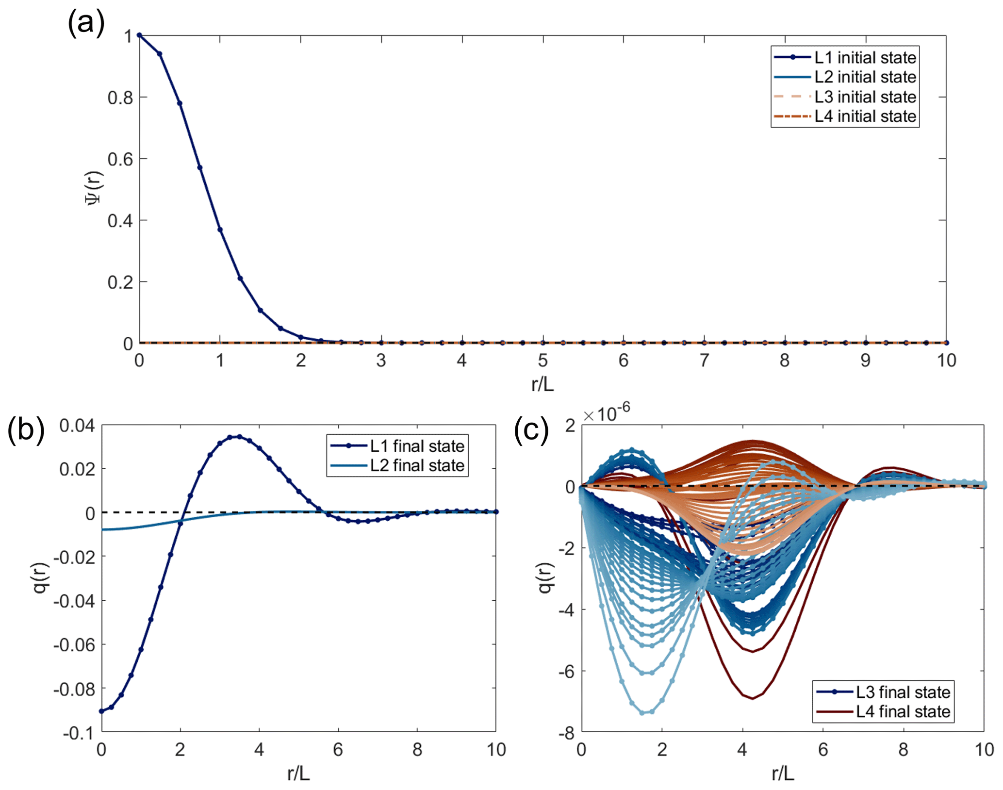
Figure 3 (a) Radial profiles of the initial states of the streamfunctions for the four levels (L_i, where $i=\mathrm{1},\mathrm{\dots },\mathrm{4}$). Radial profiles of the final states of potential vorticity with respect to (b) the first two levels and (c) the remaining levels for all configurations, with shades of blue representing the third level and shades of red representing the fourth level.

3.1 Qualitative validation

In layered QG models, the interfacial deformation radii are determined using layer-wise stratification parameters. Thus, using level thicknesses, the Coriolis parameter, and densities, it is possible to evaluate the internal instance of the interfacial deformation radius ($L_{\mathrm{d}}^j=\sqrt{g_j^{\prime }{h}_j}/f$) for the jth level, which is a baroclinic Rossby radius of deformation, taking into account reduced gravity and the relative thickness of the levels (LeBlond and Mysak, 1978). In continuously stratified systems, the modal deformation radii decrease with increasing mode number (Nittis et al., 1993). Higher modes are associated with shorter vertical wavelengths and more zero crossings in their vertical structure functions. On the other hand, in a layered model, the radii tend to increase toward the bottom of the water column due to reduced gravity, and the thickness of the layers changes with depth. This is easily explained in a two-layer model (LeBlond and Mysak, 1978; Carton et al., 2014), but in our case, it depends on the nonlinear coupling among the different levels, resulting in a locally equivalent barotropic dynamic.

The first level exhibits L_d≃15 km, while the second level exhibits L_d≃44 km, consistent with the typical internal radius values for the first oscillation modes reported in the literature (Carton et al., 2014; Nittis et al., 1993). The third- and fourth-level radii measure ∼ 40–120 km, as shown in Fig. 4a, peaking at ∼90 km, which aligns with observations from the Ionian Sea in which the only persisting scales are attributable to gyres at intermediate and deep levels (Nittis et al., 1993; Robinson et al., 1991; Pinardi and Masetti, 2000). Of course, these high values are dependent on the abrupt density variations considered when using the piecewise constant density in the model (Fig. 2b). However, the fact that they fall within the same order of magnitude as different observations suggests that we are not deviating too much from reality.

To overcome the data paucity and make use of the available resources and former observations, we found that the only parameter capable of providing a reasonable comparison between very different observations and our model data was the phase speed of the internal modes (LeBlond and Mysak, 1978). In Fig. 4b, we compare the phase speed values from our model with two available observations conducted in the Ionian Sea deep layer: one concerns the abyssal vortex identified by Rubino et al. (2012), and the other concerns the blue-shift peak observed in the current spectrum of NEMO-SN1 in the same period (Fig. 1a). The phase speed values from our model account for both the scales of the parameters and the timescale of the integration to yield a more realistic speed value ($v_{\mathrm{p}}=\sqrt{g_j^{\prime }{h}_j}\cdot (H/LT{f}_{\mathrm{0}})$). The phase speed is v_p≃5.86 cm s⁻¹ for the first level, v_p≃16.4 cm s⁻¹ for the second level, ∼ 10–50 cm s⁻¹ for the third level, and ∼ 10–40 cm s⁻¹ for the fourth level. The estimates from Rubino et al. (2012) take into account the background flow (which travels in a direction opposite to that of the vortices depicted in Fig. 3a of their paper) and the Rossby radius (as shown in Table 1 of their paper) to generate a scaling factor comparable to ours ($v_{\mathrm{p}}=(\mathit{\lambda }/T+\mathrm{bkg})\cdot (H/R{r}_{\mathrm{vortex}})\simeq \mathrm{29.4}$ cm s⁻¹, where λ represents the wavelength, T represents the period of the first anticyclone, and “bkg” stands for background). The NEMO-SN1 phase speed estimate is based on the blue-shifted peak in the current spectra, as shown in Fig. 1a, and is expressed as $v_{\mathrm{p}}=\mathit{\omega }/k\simeq \mathrm{23.5}$ cm s⁻¹ (i.e., frequency over wavenumber).

Figure 4 (a) Relative frequency of the values of internal deformation radii for the different configurations of the third and fourth levels. The values of the first- and second-level radii are also presented. (b) Relative frequency of Rossby phase speed values for the different configurations of the third and fourth levels. The values of the first- and second-level speeds (black) are also presented. Additionally, phase speed estimates for observed vortices in the Ionian Sea (red), sourced from Rubino et al. (2012), are shown, as well as those for current time series from NEMO-SN1 (blue).

4 Results and discussion

The potential vorticity that propagates through the levels significantly differs when the relative thicknesses of the bottom levels are altered (Fig. 3c). If the relative thickness of the different levels had a negligible impact on all possible configurations, according to the design of our numerical model, no changes would occur, and the potential vorticity would remain confined in its original state. However, the second-order stretching term (Eq. 8b), which connects the water column through the density differences between the levels and their different thicknesses, seems to have a bigger impact on some configurations of the relative thicknesses of the third and fourth levels.

To investigate whether there were any typical configurations, we plotted the final states in the $(q_i,q_{i+\mathrm{1}})$ parameter space ($i=\mathrm{1},\mathrm{3}$), chosen because the potential vorticities at each level directly affect system stability (Bashmachnikov et al., 2017), creating a sort of stability phase diagram, which, however, turned out to be quite complex (Fig. 5a and b). In Fig. 5a, the final potential vorticity of the first two levels, which are never perturbed, is not exactly the same for all configurations. There is a shift in some cases, while the overall pattern remains the same, reflecting the radial distribution seen in Fig. 3. This suggests that changes in the configurations of the third- and fourth-level thicknesses influence the transmission of potential vorticity through the bottom layers of the water column (and vice versa). In particular, there is more transmission when $h_{\mathrm{3}}/h_{\mathrm{4}}=\mathrm{0.74}$, 0.77, 1, 1.1, 1.2, 1.3, 1.4, 1.5, 1.6, 3.6, 4.1, or 4.4 (the “bumps” in Fig. 5a), corresponding to larger features of the bottom-level potential vorticity (Fig. 5b).

In Fig. 5b, it can be seen how the potential vorticity of the bottom levels changes drastically in response to varying thicknesses, without showing regularity. However, in the 2D plot, a trend emerges where the vorticity of the third and fourth levels tends to align with the spiral pattern of the first two levels when the first and last configurations are applied (dark blue and dark red). This tendency is disrupted by nonlinearity as we approach $h\mathrm{3}/h\mathrm{4}=\mathrm{1}$, which corresponds to the “bumps” pertaining to the first two levels, as mentioned earlier. This indicates that the strong nonlinear coupling of the relative thickness and density of the deep layers affects the entire water column.

Figure 5 Final-state potential vorticity in parameter space ($q_i,q_{i+\mathrm{1}}$; $i=\mathrm{1},\mathrm{3}$) for (a) the first and second levels and (b) the third and fourth levels, meshed with relative thickness in the vertical direction (the ticks are equispaced for readability since there are some extra configurations). Contours are colored according to the configurations of bottom-level thickness. The inset in the top-right corner of each panel shows the same data in 2D. The chosen plotting angle makes the inversion nodes for $h_{\mathrm{3}}/h_{\mathrm{4}}=\mathrm{0.67}$ and $h_{\mathrm{3}}/h_{\mathrm{4}}=\mathrm{4.1}$ evident.

Examining the spatial fields at the limit values of $h_{\mathrm{3}}/h_{\mathrm{4}}$ – specifically, the lowest, highest, and about-critical values – it can be seen that vorticity penetrates more into the third level when $h_{\mathrm{3}}/h_{\mathrm{4}}\ll \mathrm{1}$ (Fig. 6a) and more into the fourth level when $h_{\mathrm{3}}/h_{\mathrm{4}}\gg \mathrm{1}$ (Fig. 6d). Before the threshold transition, the third level exhibits higher potential-vorticity values than the fourth (Fig. 6b). After the transition, the potential vorticity in the third and fourth levels is almost the same (Fig. 6c), and it can be seen, particularly at the outer corners of the vortex in the third level, how the rotational direction inverts (Fig. 6b and c).

Figure 6 Spatial fields of potential vorticity in the four-level case for (a) $h_{\mathrm{3}}/h_{\mathrm{4}}=\mathrm{0.15}$, (b) $h_{\mathrm{3}}/h_{\mathrm{4}}=\mathrm{0.77}$, (c) $h_{\mathrm{3}}/h_{\mathrm{4}}=\mathrm{0.84}$, and (d) $h_{\mathrm{3}}/h_{\mathrm{4}}=\mathrm{6.7}$. The color bar ranges are different for different levels.

This behavior is not reproduced in the two-level (Fig. 7) and three-level (Fig. 8) cases, which were simulated under the same conditions as the four-level case and employed the same thickness ratios for the bottom levels. In Figs. 7 and 8, it can be seen how the coupling slowly transfers more potential vorticity to the bottom level.

Figure 7 Spatial fields of potential vorticity in the two-level case for (a) $h_{\mathrm{1}}/h_{\mathrm{2}}=\mathrm{0.15}$ and (b) $h_{\mathrm{1}}/h_{\mathrm{2}}=\mathrm{3.18}$. The color bar ranges are different for different levels.

Figure 8 Spatial fields of potential vorticity in the three-level case for (a) $h_{\mathrm{2}}/h_{\mathrm{3}}=\mathrm{0.15}$ and (b) $h_{\mathrm{2}}/h_{\mathrm{3}}=\mathrm{3.18}$. The color bar ranges are different for different levels.

Figure 9 Streamfunction projection on the barotropic and baroclinic modes in the physical plane for (a) $h_{\mathrm{3}}/h_{\mathrm{4}}=\mathrm{0.15}$, (b) $h_{\mathrm{3}}/h_{\mathrm{4}}=\mathrm{0.77}$, (c) $h_{\mathrm{3}}/h_{\mathrm{4}}=\mathrm{0.84}$, and (d) $h_{\mathrm{3}}/h_{\mathrm{4}}=\mathrm{6.7}$. The color bar ranges are different for different modes.

When exploring the modal projection of the streamfunction, the impact of varying stratification configurations on the system becomes even more apparent (Fig. 9). The modes are computed from Eq. (8b) when q=0, using the separation of variables, and then the evolved streamfunction is projected onto the eigenvector basis (Smith and Vallis, 2001; Katsman et al., 2003). There is a conversion between the first and second baroclinic modes that alters the sign of the barotropic mode for values before the critical transition (Fig. 9a and b). The first and second modes are more affected by the stratification configuration. The first mode has more modal energy near the transition (Fig. 9b and c), while the second mode is more energetic away from the transition (Fig. 9a and d) and has different signs. On the other hand, the third mode is almost identical across all configurations, exhibiting slightly more or less modal energy away from transition (Fig. 9a and d).

This critical behavior becomes more evident when choosing more appropriate variables to investigate the nonlinear region, i.e., the ratios between the vorticities of the third and fourth levels and the corresponding thickness ratios (Fig. 10). In particular, Fig. 10a shows the ratio between the sign-preserving maximum absolute values of the third- and fourth-level potential vorticities, which can be defined, using x as a generic variable, as

$$\begin{array}{}\text{(13)}& \mathrm{sign}\left(\min \right(x)+\max (x\left)\right)\cdot \max \left(\right|\min \left(x\right)|,|\max \left(x\right)\left|\right).\end{array}$$

As the thickness of the third level increases (and subsequently the thickness of the fourth level decreases), the vorticity signal tends to initially rotate in the same direction until it reaches a critical ratio below $h_{\mathrm{3}}/h_{\mathrm{4}}=\mathrm{1}$, at which point a sort of phase transition occurs (Parisi and Shankar, 1988). This behavior is not present in either the three-level case (Fig. 10b) or the two-level case (Fig. 10c), where the potential vorticity slowly transitions to the bottom level in a monotonic manner.

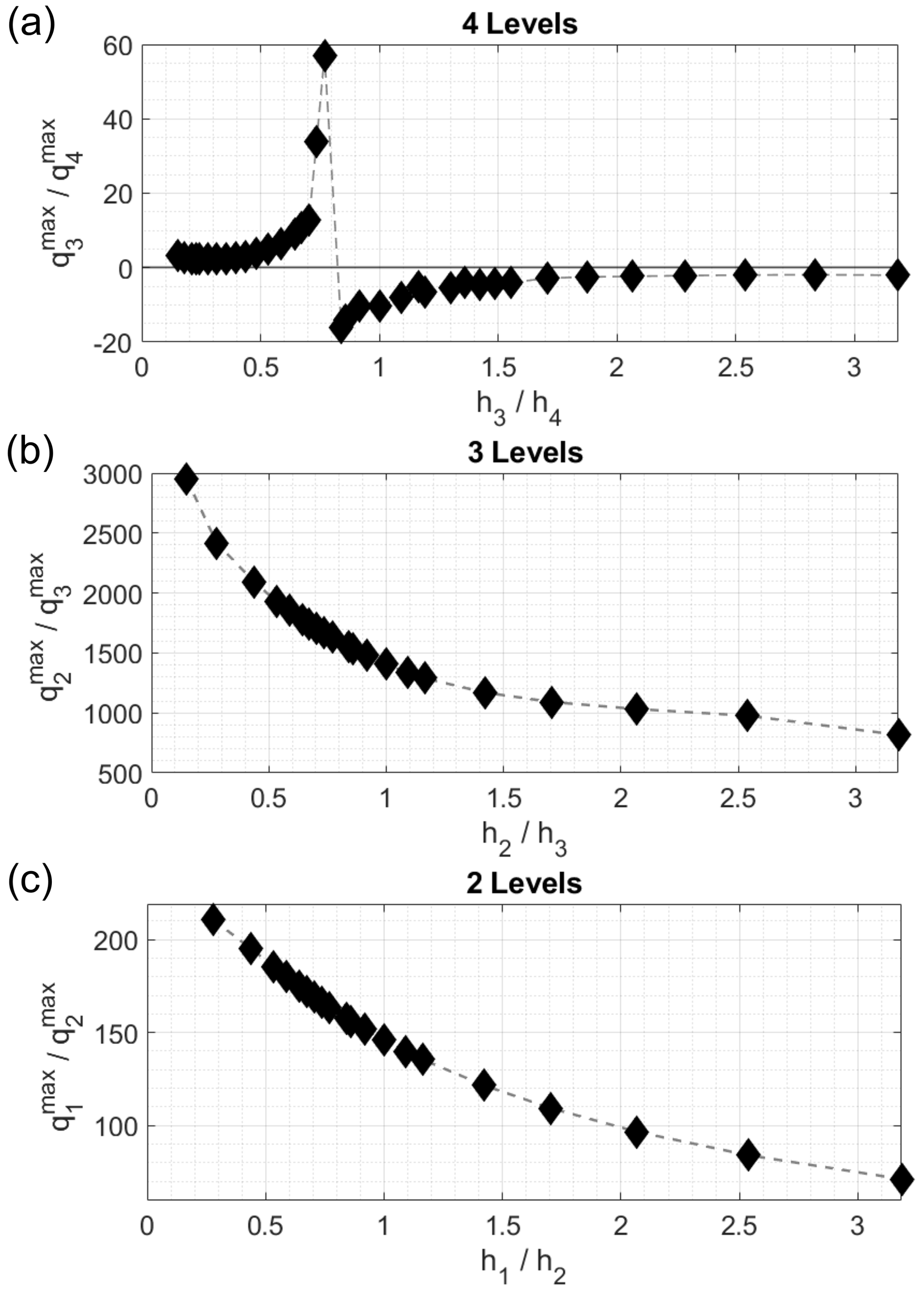
Figure 10 The ratios of the sign-preserving maximum absolute values of the potential vorticities for the (n−1)th and nth levels versus the thickness ratios for the (a) four-level case, (b) three-level case, and (c) two-level case.

In particular, the critical ratio found for the four-level case has a value of ∼0.77, which is close to the value of 0.8, where the marginal stability curves meet in the two-level case, as reported by Benilov (2003). This is also the configuration in which the sign of the barotropic mode's streamfunction changes (Fig. 9b). The presence of such critical configurations serves as a retrospective justification for the time parameterization used (i.e., exploring the stable configuration independently of time evolution) since this approach would lead to non-convergence of the algorithm in an evolutionary model. The potential-vorticity signal thus increases in the fourth level, and the rotation direction inverts. Therefore, regardless of stronger dissipation, forcing, and other instabilities considered in a more accurate description of the flow dynamics, the net effect of deep-stratification variability reshapes the structure of the mean circulation and mass distributions throughout the entire water column.

This stratification-driven reshaping can have important implications for understanding realistic vortex stability. It has been suggested that a weak co-rotating circulation in the lower layer of a vortex can stabilize the vortex, providing a plausible explanation for the observed longevity of oceanic vortices (Dewar and Killworth, 1995; Benilov, 2005). Moreover, Benilov (2005) shows that instead of assuming deep circulation has the same profile as the upper-layer vortex (like in Dewar and Killworth, 1995, and Katsman et al., 2003), it is more realistic to assume constant potential vorticity in the deep layers. This implies that the circulation resulting from upper-layer displacement is always co-rotating, contributing to its stabilization. Alternatively, as proposed by Sutyrin (2015), the presence of a middle layer with uniform potential vorticity can weaken vertical coupling and enhance vortex stability.

To explore the stability of the system (which, in our case, has a small-order effect but still deserves attention), we used the Benilov (2003) definition for vortex stability inside the ith layer, given by the sign of the potential-vorticity radial derivative with respect to the azimuthal velocity of the vortex ($\mathrm{d}{Q}_i/\mathrm{d}r\to -V_i$). Figure 11 shows the radial derivatives of potential vorticity for all the levels. For the first two levels (Fig. 11a and b), the radial derivative of the streamfunction, i.e., the radial velocity, is also observed. However, for the sake of readability, the latter cannot be included in the same plot as the other radial-derivative data as it also depends on the configuration (Fig. 11c and d).

Figure 11 Radial derivative of potential vorticity for the (a) first, (b) second, (c) third, and (d) fourth levels. The dashed line indicates the zero line, and the dashed–dotted line in panels (a) and (b) shows the radial derivative of the streamfunction.

The vortex in the first and second levels (Fig. 11a and b) is stable at the center but becomes unstable at the borders, which is expected due to dissipation. Overall, the trends for the third and fourth levels are very different and not comparable, except with respect to certain configurations. In particular, configurations with a smaller third level (smaller than 450 m) have the same sign (indicating a very unstable vortex), and configurations with h₃=975, 1000, 1150, 1200, 1250, 1300, 1350, 1375, 1400, 1800, 1850, or 1875 have opposite signs (indicating a very stable vortex). Even in the absence of disturbances, the equilibrium state is not stable for all configurations of levels.

Regarding the overall stability of the vortex throughout the water column, one can consider a criterion similar to that of Rayleigh’s inflection point thereom – i.e., the vortex is stable when the sign of $\mathrm{d}{Q}_i/\mathrm{d}r$ does not change in the other layer (McWilliams, 2006). Comparing the signs of $\mathrm{d}{Q}_i/\mathrm{d}r$ among the levels (Fig. 11), it becomes evident how changes in deep stratification can influence the stability of the potential-vorticity profiles. This is particularly noticeable for the second level in relation to the third, which, in turn, is strongly coupled with the fourth. This, of course, is a reflection of the change in the potential-vorticity sense of rotation highlighted previously.

The fact that the layers couple through stratification, instantaneously creating a circulation pattern in the layers below (with a rotation sign related to the relative thickness of the layers), could be an important factor affecting the stability/instability of vortices. In a QG framework, when considering ocean-like stratifications, i.e., accounting for the upper-layer pycnocline while assuming an abyss at rest, the equilibration mechanisms for vortices are typically set a priori (Smith and Vallis, 2001). Our results suggest that introducing a little complexity to the vertical structure of the abyssal layers could provide a more realistic picture without imposing a priori conditions for stability. However, the contribution of the deep stratification we found is relatively small when comparing the potential-vorticity values in the upper layers with those in the lower layers. To further test the implications and possible impacts, we examined the vortex evolution under the same conditions, introducing periodic radial perturbations into the streamfunction (Eq. 12). This can be defined as $r=r\cdot (\mathrm{1}+\mathit{ϵ}\cos \mathrm{2}\mathit{\theta })$, where θ is the azimuthal angle and ϵ is a small parameter, allowing for variation in ψ with a finite but small amplitude. We consider 2θ since, in a single-level case, this choice leads to a known scenario involving the dipolar breaking of the original vortex patch, providing a reference point for interpreting the results in the four-level case (Carton et al., 2014; Cushman-Roisin and Beckers, 2011).

Figure 12 Time evolution of the spatial fields from the perturbed four-level case across several iterations, with a bottom-level thickness ratio of $h_{\mathrm{3}}/h_{\mathrm{4}}=\mathrm{0.15}$. The columns are organized by level and the rows by iteration time. A zoomed-out view of the grid allows us to better capture the evolution shape. Note also that the color bar has a consistent time range for each level, though it differs from level to level.

Figure 13 Time evolution of the spatial fields from the perturbed four-level case across several iterations, with a bottom-level thickness ratio of $h_{\mathrm{3}}/h_{\mathrm{4}}=\mathrm{0.77}$. The columns are organized by level and the rows by iteration time. A zoomed-out view of the grid allows us to better capture the evolution shape. Note also that the color bar has a consistent time range for each level, though it differs from level to level.

In Figs. 12 and 13, the vortex patch evolutions for bottom-level thickness ratios of $h_{\mathrm{3}}/h_{\mathrm{4}}=\mathrm{0.15}$ and $h_{\mathrm{3}}/h_{\mathrm{4}}=\mathrm{0.77}$, respectively, are shown. The overall evolution of the first level is different from what was expected. The presence of the levels below generates certain effects through potential-vorticity conservation; however, compared to the non-perturbed case, these effects are greater in terms of both the instability of the patch evolution geometry and the potential-vorticity magnitude. As observed in the non-perturbed case, the nonlinear coupling automatically creates a nonzero vorticity in the second level, which then propagates to the bottom levels. The evolution of a vortex interacting with a vortex patch in the middle level has been studied before (Sokolovskiy et al., 2020), and it typically leads to the dipolar breaking of the upper-level vortex. Instead, here, we observe the formation of a tripole in the second level as well. In the third and fourth levels, small vortices form that remain aligned with the initial vortex position. Over longer timescales, the vortices continue to rotate until complete dissipation occurs since there is no background flow for them to interact with. The bottom levels contribute to dissipation by acting as sinks of potential vorticity, as clearly shown by the intensification illustrated in the bottom panels of Fig. 12.

Figure 14 Streamfunction projection on the barotropic and baroclinic modes in the physical plane for (a) $h_{\mathrm{3}}/h_{\mathrm{4}}=\mathrm{0.15}$ and (b) $h_{\mathrm{3}}/h_{\mathrm{4}}=\mathrm{0.77}$, corresponding to the perturbed four-level case from the last iterations shown in Figs. 12 and 13. The color bar ranges are different for different modes.

The most interesting outcome is that the critical behavior observed in the stationary case is also reproduced in the first two levels when perturbation is considered. In fact, when $h_{\mathrm{3}}/h_{\mathrm{4}}=\mathrm{0.77}$, which approaches the critical transition in the stationary case (Fig. 10a), the rotation direction also inverts in the first levels (Fig. 13). Moreover, the potential vorticity that reaches the bottom levels is significantly higher in this case than in the stationary case, thus reassuring us that the presence of deep stratification can indeed lead to a non-negligible impact when considering more realistic evolution.

This is consistent with the barotropic modal structure of the stationary case (Fig. 9) and can be observed in the corresponding modal projection for the perturbed case (Fig. 14). The signs of the modes in the stationary and perturbed cases are the same; however, the perturbation changes the modal structure, modulating the energy distribution. This perturbation highlights the strong connection between stratification configuration and the first two baroclinic modes (Fig. 14). During the critical transition, in addition to the sign and orientation of the barotropic mode changing, the first and second baroclinic modes behave very differently, and a symmetry in the modal structure around the critical value emerges. The second modal structure in Fig. 14a is reproduced by the first mode for the critical configuration (Fig. 14b), while the first mode in Fig. 14a and the second mode in Fig. 14b are completely different in terms of both shape and sign. The third mode appears unchanged, as it does in the stationary case.

Therefore, even when considering regular perturbations, the mere presence of a dense deep layer, which depends on the thickness of the deep layer relative to the upper layer, can act as either a stabilizer or a disruptor of ocean vortices. This is also relevant in our case study area, where abyssal vortices exist and were observed by Rubino et al. (2012) in 2002–2003, with in situ data depicting a relative stratification of $h_{\mathrm{3}}/h_{\mathrm{4}}=\mathrm{800}/\mathrm{1500}=\mathrm{0.53}$. This value, as seen in Fig. 5c, corresponds to a higher vorticity content in the third level and co-rotation of the third and fourth levels; thus, it is one of the configurations ensuring the vortex stability condition discussed earlier (Benilov, 2003).

This contribution of deep stratification to deep-sea variability, though small, can have important impacts when integrated over time in energy budgets. The deep sea varies on small scales compared to the rest of the ocean, but even small variations can have cascading impacts. This is seen, for example, in the EMT, during which variations of ∼0.2 °C in temperature and ∼0.1 psu in salinity in the abyss (Artale et al., 2018) resulted in abrupt changes in the circulation patterns of the Mediterranean Sea.

5 Conclusions

We applied a quasi-geostrophic level model to a two-dimensional ocean, featuring four nonlinearly coupled layers and observation-based parameters, to investigate the role of abyssal stratification in the rearrangement of potential vorticity through the water column. The transmission and stabilization of potential vorticity through the bottom layer depend on the relative thicknesses and stratification of the layers, which have proven to be critical factors in reshaping the circulation patterns of the water column. The dense and stable deep layer observed in the Ionian Sea since the late 1990s provides an example of the baroclinic exchange from kinetic to potential energy along the vertical direction (Artale et al., 2018; Manca et al., 2006; Klein et al., 1999; Li and Tanhua, 2020; Giambenedetti et al., 2023). This example reflects a wider trend observed in the global oceans, as noted in the latest Intergovernmental Panel on Climate Change (IPCC) reports, which state that ocean stratification has increased substantially over the past decades, even at great depths (Li et al., 2020).

The formulation of our model did not follow that of the usual layer models employed in studies of vortex stability (Sokolovskiy, 1997; Carton et al., 2014; Katsman et al., 2003) or potential-vorticity propagation from the surface (Smith and Vallis, 2001; Zeitlin, 2018) because we were focused neither on the evolution of a perturbed vortex across short timescales nor on higher-order processes, such as those involved in the upper layers. Instead, we wanted to investigate the problem from an upside-down point of view, aiming to understand the impact of long-timescale stratification changes in the abyss, such as those observed in the available data, on the potential vorticity structure in the water column. Hence, we used a time parameterization approach, analyzing a set of stationary states to study the nonlinear system's evolution over a decade.

The simplifications and assumptions made, however, proved to provide a realistic, albeit more qualitative than quantitative, representation when compared with different observations. In fact, the Rossby internal radii from our model are consistent with the Ionian Sea circulation trends, and the phase speed values estimated from available observations are of the same order of magnitude as those from our model (Fig. 4). Moreover, the time parameterization of the stratification evolution was justified a posteriori by the finding of critical ratios of bottom-level thicknesses (Fig. 5c).

We found that as the thickness of the denser bottom layer decreases, the potential-vorticity signal tends to initially rotate in the same direction as the above levels until the ratio between the thicknesses of the last two levels falls below a critical value of 1, at which point a sort of phase transition occurs. The potential-vorticity signal thus increases in the bottom level, and the rotation direction inverts. This critical behavior is not present when considering fewer levels (Fig. 10), suggesting that the conventional two-layer Ionian Sea system, discussed in the literature, is too simplistic for a complete representation of all processes in the ocean water column (Rubino et al., 2020; Gačić et al., 2021). Moreover, the impact of this critical behavior extends to the surface layers; in fact, the conversion between the first two baroclinic modes alters the sign of the barotropic mode (Fig. 9), and the effects of this instability on the upper level are evident when perturbing the evolution of the vortex. Indeed, we observe that near the critical values of thickness ratios pertaining to the bottom levels found in the non-perturbed case, the rotation of the first level also inverts (Figs. 12 and 13).

Therefore, regardless of stronger dissipation, forcing, and background flow, as well as other instabilities considered in a more accurate description of the flow dynamics, the net effect of deep-stratification variability reshapes the structure of the mean circulation and mass distributions throughout the entire water column.

The stratification-induced inversion we found for certain configurations of level thickness is also consistent with local observations from the Ionian Sea, as can be seen, for example, in the hodographs in Fig. 1a and b. The deep-layer stratification in the Ionian Sea changed drastically during the EMT, when the continuous entrainment of warmer and saltier Aegean waters favored instabilities and heat transfer through diffusion and turbulent mixing. After a few decades, mixing due to the concurrence of different properties (e.g., tides, internal waves, topography, and morphology) homogenized the bottom layer in the Ionian Abyssal Plain.

We demonstrated the crucial role of stratification in directing the rotation of potential vorticity generated at the interface between layers of different densities, and we showed that the entire water column engages in abyssal dynamics. This can play a role in stabilizing the propagation of Rossby waves, which, in turn, affects the sub-surface circulation. Further, it highlights the impact of the bottom layers on the vertical structure, which may have interesting implications for the redistribution of energy stored in the deep sea, warranting further investigation.

Our findings provide insight into how deep variability is connected with intermediate and surface dynamics through vertical stratification. We suggest that this should be considered in more comprehensive models, particularly when accounting for topographic effects and their interaction with a more realistic stratification than that discussed in the present work, as it could yield interesting outcomes.