Mechanisms and intraseasonal variability in the South Vietnam Upwelling, South China Sea: the role of circulation, tides, and rivers

Summer monsoon southwest wind induces the South Vietnam Upwelling (SVU) over four main areas along the southern and central Vietnamese coast: upwelling offshore of the Mekong shelf (MKU), along the southern and northern coasts (SCU and NCU), and offshore (OFU). Previous studies have highlighted the roles of wind and ocean intrinsic variability (OIV) in intraseasonal to interannual variability in the SVU. The present study complements these results by examining the influence of tides and river discharges and investigates the physical mechanisms involved in MKU functioning.

MKU is driven by non-chaotic processes, explaining its negligible intrinsic variability. It is triggered first by the interactions of currents over marked topography. The surface convergence of currents over the southwestern slope of the Mekong shelf induces a downwelling of the warm northeastward alongshore current. It flows over the shelf and encounters a cold northwestward bottom current when reaching the northeastern slope. The associated bottom convergence and surface divergence lead to an upwelling of cold water, which is entrained further north by the surface alongshore current.

Tides strengthen this circulation-topography-induced MKU through two processes. First, tidal currents weaken the current over the shallow coastal shelf by enhancing the bottom friction. This increases the horizontal velocity gradient and hence the resulting surface convergence and divergence and the associated downwelling and upwelling. Second, they reinforce the surface cooling upstream and downstream of the shelf through lateral and vertical tidal mixing. This tidal reinforcement explains 72 % of MKU intensity on average over the summer and is partly transmitted to SCU through advection. Tides do not significantly influence OFU and NCU intensity. Mekong waters slightly weaken MKU (by 9 % of the annual average) by strengthening the stratification but do not significantly influence OFU, NCU, and SCU. Last, tides and rivers do not modify the chronology of upwelling in the four areas.

1 Introduction

The South Vietnam Upwelling (SVU) develops in the South China Sea (SCS) along and off the Vietnamese coast under the influence of the summer monsoon southwest wind (Xie, 2003; Dippner et al., 2007). It is a major component of the SCS ocean circulation and influences the local climate (Xie, 2003; Zheng et al., 2016; Yu et al., 2020) as well as biological activity and fishing resources (Bombar et al., 2010; Liu et al., 2012; Loisel et al., 2017; Loick-Wilde et al., 2017; Lu et al., 2018).

The SCS circulation along and off the central and southern Vietnamese coast is characterized by a southern anticyclonic circulation and a northern cyclonic circulation. They form an eddy dipole and are associated with northeastward and southward boundary alongshore currents, respectively (Wyrtki, 1961; G. Wang et al., 2006). Recent studies showed that SVU develops over four main areas (highlighted in Fig. 1) driven by different mechanisms (Da et al., 2019; Ngo and Hsin, 2021; To Duy et al., 2022; Herrmann et al., 2023). The northeastward and southward boundary currents converge near ∼14° N, forming the summertime eastward jet (SEJ). This offshore current separation induces the southern coastal component of the SVU, hereafter called SCU. Similar upwelling can develop along the northern coast (NCU), induced by the formation of seaward currents through the convergence of alongshore currents associated with small coastal eddies. Beside those Ekman-transport-driven coastal upwellings, an Ekman-pumping-driven offshore upwelling (OFU) develops north of SEJ. Last, To Duy et al. (2022) and Herrmann et al. (2023) revealed the existence of an upwelling that develops over the Mekong shelf (MKU), whose physical mechanisms have yet to be explained.

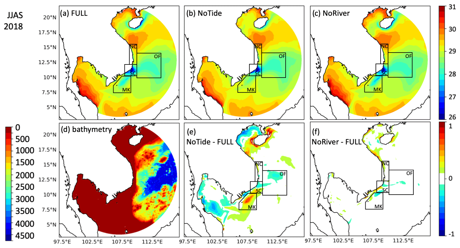
Figure 1 Ensemble average summer SST in June–September 2018 from the FULL (a), NoTide (b), and NoRiver (c) ensembles and the difference between the NoTide and FULL (e) and the NoRiver and FULL (f) ensembles [°C]. (d) Bathymetry of the domain [m]. Colour bars for panels (a)–(c) and (e)–(f) are provided at the top and bottom right, and the colour bar for panel (d) is at the bottom left. Upwelling areas have the following names and coordinates: boxNC (12.2–15.5° N, 108.7–109.9° E), boxSC (10.3–12.2° N, 108–109.9° E), boxOF (10–14° N, 109.9–114° E), and boxMK (at depth >17 m; 7.5–10.3° N, 106–109° E).

The SVU shows strong variability, from the daily and intraseasonal scales to the interannual scales. Wind is a major factor in this variability at different scales. Over the last 2 decades, numerous studies have showed the effects of wind and the El Niño–Southern Oscillation on the interannual variability in the large-scale circulation formed by the SEJ and eddy dipole and the effects on the interannual variability in the SVU intensity (Kuo et al., 2004; Y. Wang et al., 2006; Li et al., 2014; Da et al., 2019; Ngo and Hsin, 2021; To Duy et al., 2022): stronger (weaker) summer monsoon southwest wind enhanced (weakened) during La Niña (El Niño) events induces more (less) intense SEJ and SVU than average. Only a few studies have focused on the SVU variability at the intraseasonal scale. Isoguchi and Kawamura (2006) and Xie et al. (2007) showed that wind, itself strongly driven by the Madden–Julian Oscillation at the intraseasonal summer scale but also by tropical storms, is a major driver of SVU daily variability. Herrmann et al. (2023) more specifically showed that wind is the main driver of daily variability in SEJ and in SCU, OFU, and MKU. They showed that NCU variability was rather driven by the strength of the large-scale circulation at the intraseasonal scale: the well-established circulation and southward boundary current during the core of summer prevent the development of seaward currents along the northern coast and hence the development of NCU. NCU rather develops at the beginning and end of the summer when this circulation is weaker, allowing small-scale eddying structures and seaward currents to develop.

Recent modelling studies moreover revealed the high impact of ocean intrinsic variability (OIV) on SVU. OIV is mainly related to the intense activity of (sub-)mesoscale structures and eddies of strongly chaotic nature in the SCS (Ni et al., 2021; Xiu et al., 2010). Li et al. (2014) first suggested that OIV could contribute 20 % of the SEJ interannual variability. Da et al. (2019) and To Duy et al. (2022) suggested that OIV influences the SVU interannual variability, in particular that of the OFU. To explain and quantify this impact of OIV, Herrmann et al. (2023) then performed and analysed an ensemble of high-resolution simulations for summer 2018, a year of strong SVU (Ngo and Hsin, 2021; To Duy et al., 2022). SCU and MKU are mainly driven by the strength of the SEJ, itself driven by wind intensity, and the impact of OIV is of the second order: the ratio between the ensemble dispersion and average of upwelling intensity is smaller than 10 %. This impact is slightly stronger for OFU (a ratio of 18 %) and significantly stronger for NCU (a ratio of 37 %). It is related to the spatial organization of sub-mesoscale to mesoscale structures and eddies of strongly chaotic behaviour and to their interaction with the wind curl.

The Mekong shelf receives considerable freshwater input from the Mekong River, with a monthly discharge varying between 15×10³ and 25×10³ m³ s⁻¹ during the summertime (Chen et al., 2012). It also hosts strong tidal activity. SCS is one of the few areas in the world where diurnal tides (mainly K₁ and O₁, with amplitudes of ∼30–50 cm over the open sea region; Guohong, 1986; Fang et al., 1999; Phan et al., 2019; Trinh et al., 2024) generally dominate semi-diurnal tides (mainly M₂ and S₂, with amplitudes generally smaller than 10–20 cm). M₂ amplitude and tidal currents are, however, locally similar to K₁ and O₁ in the southwestern SCS, in particular over the Mekong Delta shelf. There, the tidal amplitude of all components is stronger than over the rest of the basin (reaching ∼1 m for M₂; see the estimations by the FES2014b tidal atlas by Carrere et al., 2013, and numerical simulations in Trinh et al., 2024). The SVU may therefore be influenced by river water and tides, in particular in the MKU and SCU regions, which host the Mekong plume and strong tidal activity.

The role of the interactions between circulation, tides, rivers, and topography was examined and demonstrated in other upwelling regions, mostly based on numerical experiments. In the northern SCS in particular, several authors examined upwellings developing off the coast of Hainan Island. Lü et al. (2008) and Li et al. (2020) proved that tidal mixing induces changes in the horizontal pressure gradient and hence in circulation, which explains the development of upwelling off western and northeastern Hainan. The surface cooling is also intensified locally by the vertical tidal mixing of cold deep water with warmer shallow water (Li et al., 2020). Bai et al. (2020) moreover showed that the high-frequency variations in the western Hainan upwelling were related to both horizontal advection due to tidal currents and vertical velocity due to divergence/convergence triggered by tidal waves. Changes in horizontal density gradients and circulation induced by tidal mixing were also shown to play a major role further north, in the upwelling that develops in the lee of a coastal promontory off the Yangtze River estuary in the East China Sea (Lü et al., 2006) and in the Bohai Sea (Xu et al., 2023). Lü et al. (2006) also mentioned the role of the Yangtze river discharge. Upwelling in those regions can moreover be induced by the interactions of geostrophic circulation (Lü et al., 2006).

Despite the importance of river discharge and tidal activity in the SVU area, very few numerical studies of SVU have been based on three-dimensional models including tides and realistic river discharges and even fewer have investigated the impact of these processes. Among them, the process-oriented experiments of Chen et al. (2012) suggested that during summertime stratified conditions, tidal rectification, river discharge, and local bathymetry could intensify the northern southward and southern northeastward currents and the associated SCU. In the $\mathrm{1}/\mathrm{12}$° simulations of Da et al. (2019) using monthly climatological discharges for three rivers (Mekong, Pearl, and Red rivers) but not including tides, rivers did not have a statistically significant effect on the global SVU intensity at the interannual scale. They did, however, produce strong differences in certain years. Their statistical significance should thus be explored given the OIV effect on the SVU.

This paper follows and belongs to the ensemble of studies cited above that investigated the functioning and variability in the upwelling that develops off the Vietnamese coast, in particular through its signature of sea surface temperature (SST). The general goal of the paper is to deepen our understanding of the functioning and variability in the SVU, considering potentially important processes and aspects that were not the focus of most of the previous studies in this upwelling region: small-scale dynamics and associated chaotic variability, tides and daily river discharges, and upwelling over the Mekong shelf. This follows, in particular, the study of Herrmann et al. (2023), who quantified the impact of OIV at the intraseasonal scale based on ensemble simulations. Given the strong influence of OIV on SVU, we adopt the same probabilistic approach following Waldman et al. (2017, 2018). We now aim first to quantify and explain the influence of tides and rivers on the SVU over its four areas of development at the daily to intraseasonal scales. Second, we aim to identify the physical mechanisms responsible for MKU development. For that, we perform high-resolution reference and sensitivity ensemble simulations using the same configuration of the SYMPHONIE model as To Duy et al. (2022) and Herrmann et al. (2023), including, in particular, realistic daily river discharges and explicit tide representation.

The model, reference and sensitivity ensemble simulations, and statistical indicators are presented in Sect. 2. Results of the ensembles are statistically analysed in Sect. 3 to quantitatively assess the effects of tides and rivers on SCU, NCU, OFU, and MKU intensity. Mechanisms behind MKU are explored in Sect. 4. The robustness of our conclusions is discussed in Sect. 5. Concluding remarks and future works are given in Sect. 6.

2 Methodology and tools

2.1 The ocean model SYMPHONIE

The SYMPHONIE model (Marsaleix et al., 2008, 2019) is a three-dimensional ocean model developed by the SIROCCO group for the study of coastal and regional oceans. As explained on the SIROCCO website, “it is based on the Navier–Stokes primitive equations solved on an Arakawa curvilinear C grid under the hydrostatic and Boussinesq approximations.” Vertical mixing is parameterized according to the k-epsilon turbulence closure scheme (Rodi, 1987). The configuration used here was implemented by To Duy et al. (2022) over the Vietnamese coastal area and South China Sea region, using a standard horizontal polar grid with a resolution decreasing linearly from 1 km at the coast to 4.5 km offshore and 50 VQS (vanishing quasi-sigma) vertical levels. Figure 1 shows the limits and bathymetry of the numerical domain. Forcings are the same as used by Herrmann et al. (2023) to perform an ensemble simulation over the period 2017–2018. The atmospheric forcing is computed from the bulk formulae of Large and Yeager (2004) using the 3 h output of the European Center for Medium-Range Weather Forecasts (ECMWF) $\mathrm{1}/\mathrm{8}$° atmospheric analysis, distributed on http://www.ecmwf.int (last access: 17 August 2024). Lateral ocean boundary conditions are provided by the daily outputs of the global ocean $\mathrm{1}/\mathrm{12}$° analysis, PSY4QV3R1, distributed by the Copernicus Marine and Environment Monitoring Service (CMEMS) on http://marine.copernicus.eu (last access: 17 August 2024). The implementation of tides follows Pairaud et al. (2008, 2010), and we prescribe the same daily discharge of 36 rivers along the coast as Herrmann et al. (2023), including majors rivers such as the Mekong and Red rivers.

The ability of the model to represent the ocean dynamics and water masses of the study area, from daily to interannual scales and from coastal to regional scales, was demonstrated in detail by To Duy et al. (2022). For this, they compared a simulation performed over the period of 2009–2018, hereafter called LONG, to satellite datasets of sea surface temperature, salinity, and elevation and with in situ temperature and salinity datasets from ARGO floats; a glider; conductivity, temperature, and depth (CTD) sensors; and thermosalinograph measurements. In particular, their high-resolution simulation, together and in agreement with a careful examination of available satellite and in situ data, showed for the first time the existence of MKU and the ability of the model to represent it.

2.2 Ensemble simulations

We performed three ensemble simulations over the period of 2017–2018. The reference ensemble FULL includes rivers and tides and was already used by Herrmann et al. (2023) to examine the impact of OIV on the SVU intraseasonal variability. The additional sensitivity ensembles, NoRiver and NoTide, are identical to FULL but without river discharges and without tides, respectively. Each ensemble is composed of 10 members with perturbed initial small-scale fields of temperature, salinity, and currents, as detailed by Herrmann et al. (2023); the randomization strategy is based on the fact that most of the OIV develops at the (sub-)mesoscale related to eddies and structures of strongly chaotic behaviour (Sérazin et al., 2015; Waldman et al., 2018) that are smaller than ∼100 km in the South China Sea (Lin et al., 2020; Ni et al., 2021). For each member MXX, with XX between 09 and 18, the initial state in terms of temperature, salinity, currents, and sea surface elevation is the sum of a large-scale state and a small-scale state. The large-scale state is the same for all members, given by the large-scale state from 1 January 2017 from the PSY4QV3R1 analysis. The small-scale state differs among members and is given for member MXX from the small-scale state of 1 January 20XX from the PSY4QV3R1 analysis. Large- and small-scale states are computed applying 100 km low-pass and high-pass filters, respectively, to the PSY4QV3R1 outputs.

2.3 Indicators

We define here indicators quantifying the upwelling intensity as well as the impact of OIV and of tides and rivers. As explained by Da et al. (2019), upwelling indicators can be built based on surface wind (Ekman transport theory) or SST (see Benazzouz et al., 2014, for a review). SST-based indicators inform us about the upwelling intensity but also about the spatial distribution of upwelled water that triggers primary production at the surface. They can moreover be applied to satellite-derived SST data to study and monitor the upwelling.

2.3.1 Upwelling areas and intensity

Figure 1 shows the June–September (hereafter JJAS) mean of the ensemble average STT of the FULL, NoTide, and NoRiver ensembles. We highlight the four main areas of development of the SVU defined by To Duy et al. (2022) based on the spatial distribution of SST and upwelling intensity in the LONG simulation: boxSC and boxNC for the southern (SCU) and northern (NCU) coastal upwelling, respectively; boxOF for the offshore upwelling (OFU); and boxMK for the upwelling offshore of the Mekong Delta (MKU). Coordinates of the upwelling areas are provided in Fig. 1.

To quantify the intensity of upwelling, we use the indicators defined by Da et al. (2019), To Duy et al. (2022), and Herrmann et al. (2023). For any given point (x,y) of the domain where $\text{SST}(x,y,t)<T_{\mathrm{0}}$, the daily intensity is defined on day t as

$$\begin{array}{}\text{(1)}& {\text{UI}}_{\mathrm{d}}(x,y,t)=T_{\text{ref}}-\text{SST}(x,y,t),\end{array}$$

where T_o=27.6 °C is the threshold temperature below which upwelling happens and T_ref=29.20 °C is the reference temperature over the area outside of the upwelling (see To Duy et al., 2022, for details). For a given upwelling area B of size A_B, the daily upwelling intensity integrated over box B is given on day t by

$$\begin{array}{}\text{(2)}& \begin{array}{rl}& {\text{UI}}_{\mathrm{d},B}\left(t\right)=\\ & {\displaystyle \frac{{\iint }_{(x,y)\text{in}B/\text{SST}(x,y,t)<T_o}(T_{\text{ref}}-\text{SST}(x,y,z,t\left)\right)\mathrm{d}x\mathrm{d}y}{A_B}}.\end{array}\end{array}$$

Last, the intensity of upwelling integrated over the summer and the area B is given by

$$\begin{array}{}\text{(3)}& {\text{UI}}_{\text{JJAS},B}={\displaystyle \frac{{\int }_{\text{JJAS}}{\text{UI}}_{\mathrm{d},B}\left(t\right)\mathrm{d}t}{{\text{ND}}_{\text{JJAS}}}},\end{array}$$

where ND_JJAS=122 is the number of days over JJAS.

Figure 2 shows the area of upwelling development (highlighted by the 0.2 °C isoline of the summer average of daily upwelling index UI_d) in 2017 and 2018 for the 10 members of the FULL ensemble and from 2009 to 2018 for the LONG simulation. Figures 1 and 2 confirm that the boxes defined by To Duy et al. (2022) fully cover the upwelling development areas. MKU does not develop along the coast but ∼50 km off the Mekong Delta coastline. It thus slightly covers the Mekong plume, as highlighted in Fig. 2a by the difference between FULL and NoTide in the JJAS sea surface salinity ensemble average.

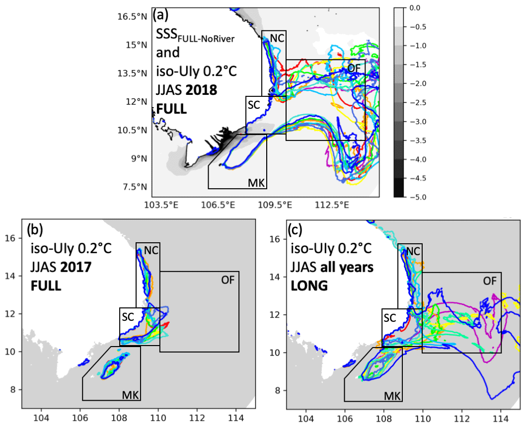
Figure 2 Ensemble average sea surface salinity in June–September 2018 from FULL (colours; a) and 0.2 °C isoline of the summer-averaged upwelling index for the 10 members of the FULL simulation in 2018 (a) and 2017 (b) and for the 10 years of the LONG simulation (c).

2.3.2 Ocean intrinsic variability

To quantify the impact of OIV on daily and yearly upwelling indexes for a given ensemble, we use the OIV indicators defined by Herrmann et al. (2023).

IV_d,B quantifies the effect of OIV on upwelling intensity over a given upwelling area at the daily scale:

$$\begin{array}{}\text{(4)}& {\text{IV}}_{\mathrm{d},B}\left(t\right)={\displaystyle \frac{{\mathit{\sigma }}_i\left({\text{UI}}_{\mathrm{d},B}\right(t\left)\right)}{\sqrt{m_i\left({\mathit{\sigma }}_t\right({\text{UI}}_{\mathrm{d},B}\left(t\right){)}^{\mathrm{2}})}}},\end{array}$$

where m_i is the ensemble mean and σ_t and σ_i the temporal and ensemble standard deviations.

IV_JJAS,B quantifies the effect of OIV on upwelling intensity at the summer scale:

$$\begin{array}{}\text{(5)}& {\text{IV}}_{\text{JJAS},B}={\displaystyle \frac{{\mathit{\sigma }}_i\left({\text{UI}}_{\text{JJAS},B}\right)}{m_i\left({\text{UI}}_{\text{JJAS},B}\right)}}.\end{array}$$

2.3.3 Effect of tides and rivers

To quantify the effect of tides and rivers on the upwelling intensity and intrinsic variability, we use the indicators defined by Da et al. (2019). We compute the relative differences Δm and Δσ between the FULL reference ensemble and the NoRiver or NoTide sensitivity ensemble of the respective mean (that quantifies the intensity) and standard deviation (that quantifies its intrinsic variability) of the 10-member vector of the yearly upwelling index:

$$\begin{array}{}\text{(6)}& {\displaystyle }\begin{array}{rl}{\displaystyle }\mathrm{\Delta }m& {\displaystyle }\left({\text{UI}}_{\text{JJAS},B}\right)=\\ {\displaystyle }& {\displaystyle \frac{m_{i,\text{SIM}}\left({\text{UI}}_{\text{JJAS},B}\right)-m_{i,\text{FULL}}\left({\text{UI}}_{\text{JJAS},B}\right)}{m_{i,\text{FULL}}\left({\text{UI}}_{\text{JJAS},B}\right)}}\times \mathrm{100},\end{array}\text{(7)}& {\displaystyle }\begin{array}{rl}{\displaystyle }\mathrm{\Delta }\mathit{\sigma }& {\displaystyle }\left({\text{UI}}_{\text{JJAS},B}\right)=\\ {\displaystyle }& {\displaystyle \frac{{\mathit{\sigma }}_{i,\text{SIM}}\left({\text{UI}}_{\text{JJAS},B}\right)-{\mathit{\sigma }}_{i,\text{FULL}}\left({\text{UI}}_{\text{JJAS},B}\right)}{{\mathit{\sigma }}_{i,\text{FULL}}\left({\text{UI}}_{\text{JJAS},B}\right)}}\times \mathrm{100},\end{array}\end{array}$$

where SIM denotes the sensitivity simulation NoRiver or NoTide. The sole values of Δm and Δσ reported in Table 1 do not allow us to quantitatively estimate whether those differences, and hence whether the effect of tides or rivers, are statistically significant. For that, we compute the p values p_m and p_σ associated with the t test (significance of the mean difference) and F test (significance of the standard deviation difference), respectively. We apply those tests to the 10-member vectors of UI_JJAS,B in the reference and sensitivity simulations and report them in Table 1. We also perform those tests at the daily scale on UI_d,B to assess the significance of the time series of ensemble average and intrinsic variability in upwelling intensity shown in Fig. 3 between reference and sensitivity simulations, highlighting in colours the periods when the differences are significant at more than 99 % (p value<0.01).

Table 1 Value of UI_JJAS,B for each member of each ensemble (columns 1 to 11); ensemble mean (11), standard deviation, (13) and their ratio IV_JJAS,B (14); and the difference between the sensitivity and reference simulations of the ensemble mean (12) and the ensemble spread (15). Last column (16): correlation c between UI_d,B in the sensitivity and reference simulations. In columns 12 to 15, UI stands for UI_JJAS,b.

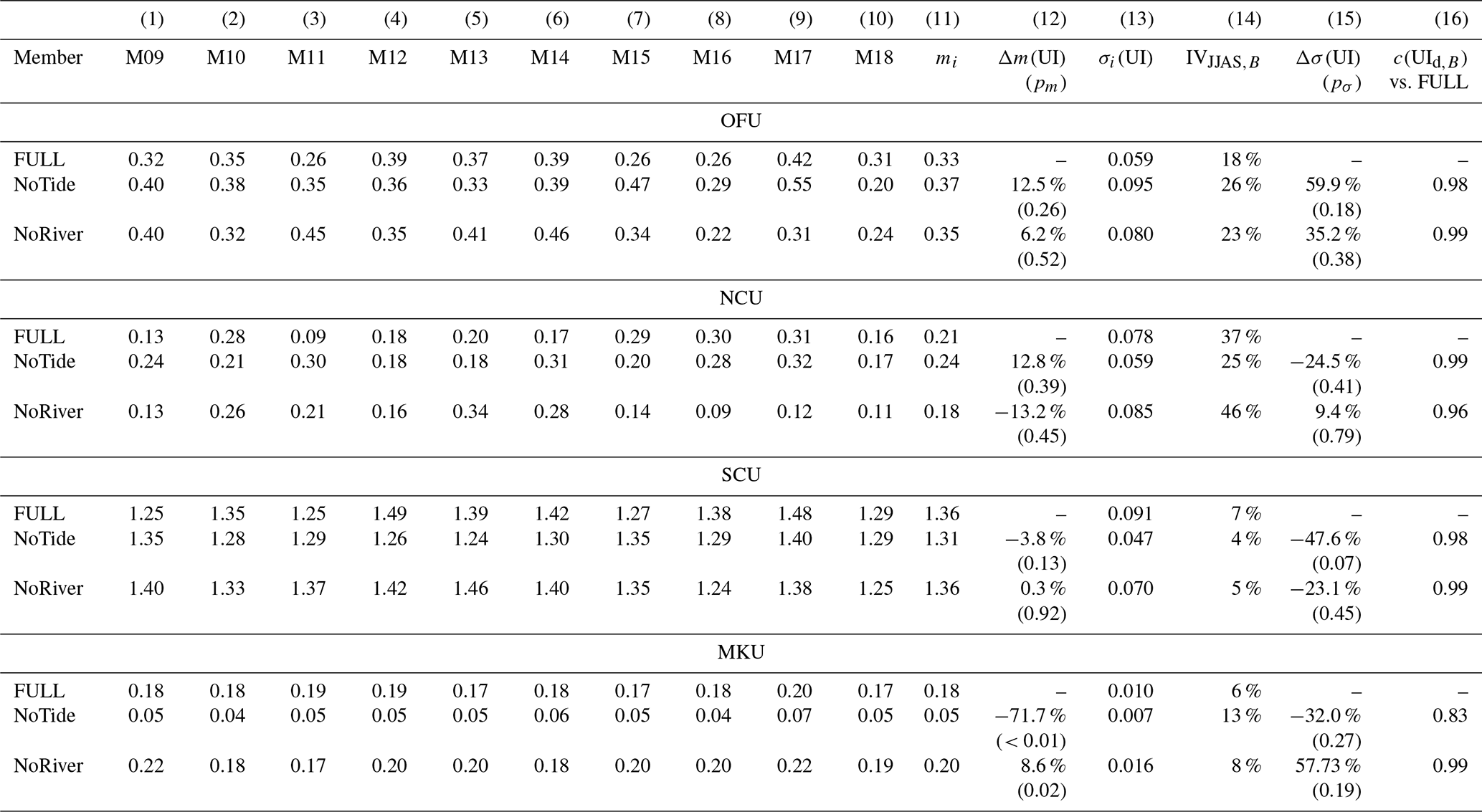
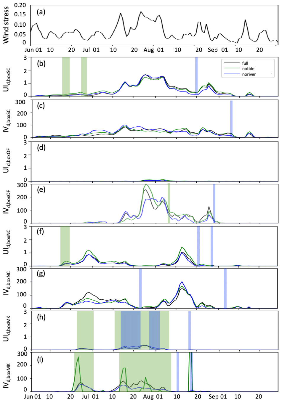
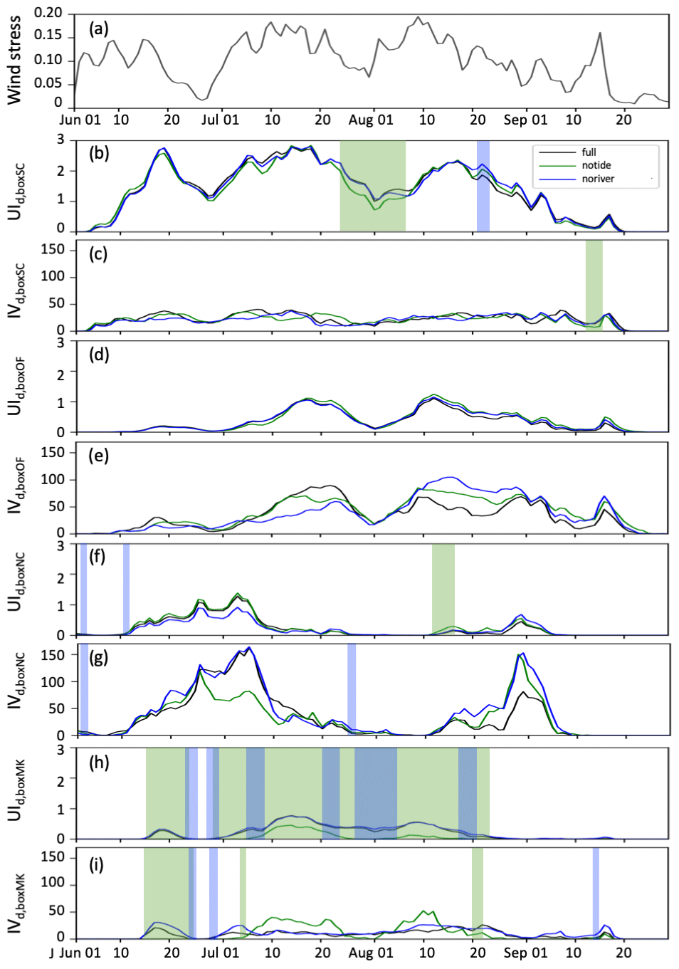
Figure 3 Daily time series in summer 2018 of averaged wind stress (a; N m⁻²) over the whole upwelling region (7.5–14° N, 106–114° E) and of the ensemble mean of UI_d,B and of IV_d,B [°C] for the FULL (black), NoTide (green), and NoRiver (blue) ensembles for NCU (b, c), SCU (d, e), OFU (f, g), and MKU (h, i). Shaded green and blue colours shows the areas where the difference between the reference FULL and sensitivity NoTide and NoRiver ensembles is statistically significant at more than 99 %.

Last, we quantify the relationship between the daily chronology of several variables over JJAS (upwelling intensity over different areas as well as wind) by computing the Pearson correlation coefficient and associated p value (that quantifies the statistical significance of the correlation) between the 122 d time series of those variables.

3 Impact of tides and rivers on the four upwelling areas

We examine the effect of tides and rivers on the four upwelling areas from a statistical point of view, based on the analysis of the daily and summer indicators introduced in Sect. 2.3. Figure 1e and f shows the maps of the difference in the ensemble average of the mean JJAS SST in NoTide and NoRiver compared to FULL. Figure 3 shows the daily time series of wind stress averaged over the entire upwelling region; of the ensemble average of UI_d,B; and of its intrinsic variability, IV_d,B, for each upwelling area, B, and each ensemble. Table 1 shows, for each ensemble and each area, the values of the summer integrated upwelling intensity, UI_JJAS,B, for all members; of their ensemble average and standard deviation; and of the differences between the sensitivity ensembles NoRiver and NoTide and the reference ensemble FULL with their levels of statistical significance.

3.1 Upwelling intraseasonal chronology

Herrmann et al. (2023) showed that the daily to intraseasonal variability in MKU, SCU, and OFU is similar and driven at the first order by the variability in wind over the upwelling region. NCU does not develop during the core of the summer but in late June and late August (Fig. 3). To Duy et al. (2022) and Herrmann et al. (2023) showed for the summers of 2009 to 2018 and summer 2018, respectively, that NCU intraseasonal variability is driven first by the large-scale circulation. The SEJ and eddy dipole that form this large-scale circulation are well established in July–August, preventing NCU from developing. They are much weaker at the beginning (June) and end (September) of summer (or during summers of very weak wind), allowing NCU to develop. This development then depends on the organization of strongly chaotic small-scale circulation and consequently shows very high intrinsic variability.

In the NoTide and NoRiver ensembles, the daily to intraseasonal chronology of upwelling intensity is very similar and is highly statistically correlated (p value<0.01) to that of the FULL ensemble for each upwelling area (Fig. 3 and Table 1, column 16). Correlation exceeds 0.96, except for MKU for the NoTide ensemble (0.83, p<0.01).

3.2 Influence of rivers

The effect of river discharge on MKU is significant, although weak. Removing river discharges increases the summer ensemble average of UI_JJAS,boxMK by 7 % (the p value associated with the differences between FULL and NoRiver is p_m=0.02; Table 1). This river effect is mainly significant during the transition period between two peaks of wind and upwelling, in particular before and after the strong mid-July and mid-August peaks (Fig. 3h): removing river discharge slightly but statistically significantly (p_m<0.01) increases the ensemble average of MKU intensity, UI_d,boxMK, by up to 30 % on 31 July. The effect of river discharge on the intrinsic variability in UI_d,boxMK is much weaker: p_σ<0.01 only during 3 d, during which MKU intensity and intrinsic variability are at any rate very weak (Fig. 3h and i).

The effect of river discharge on the ensemble average and intrinsic variability in OFU, NCU, and SCU is statistically significant neither at the summer integrated scale nor at the daily scale. The p_m and p_σ are indeed larger than 0.1 for UI_JJAS,B (Table 1, columns 12 and 15), JJAS SST differences are negligible (Fig. 1e), and p_m and p_σ<0.01 are obtained for UI_d,B only during very short periods (2–3 d maximum) and/or during periods of very weak upwelling (Fig. 3b–g).

3.3 Influence of tides

The most striking and significant effect highlighted by our sensitivity simulations is the influence of tides on MKU. This is first shown by the difference in the summer average of the SST ensemble average: the difference between NoTide and FULL reaches 0.8 °C over a large part of boxMK (Fig. 1d). The ensemble-average value of UI_JJAS,boxMK consequently decreases by 72 % (p_m<0.01) when tides are removed (Table 1). This effect of tides on the ensemble average of UI_d,boxMK intensity is highly statistically significant during the whole summer (p value<0.01, Fig. 3g). The effect of tides on intrinsic variability is, however, much weaker, with p_σ<0.01 only during a short period in June (Fig. 3i).

Tides do not significantly affect the ensemble average and intrinsic variability in SCU intensity at the summer integrated scale (p_m and p_σ>0.07; Table 1). However, at the intraseasonal scale, removing tides induces a statistically significant decrease in the ensemble average of UI_d,boxSC that can reach ∼20 % (p_m<0.01) during the transition period of relatively low SCU intensity between the July and August wind peaks (Fig. 3d). The effect of tides on the intrinsic variability in UI_d,boxSC is not statistically significant (p_σ>0.01; Fig. 3e).

Tides have a negligible influence on NCU and OFU at the summer integrated and daily scales. For those areas, the difference in JJAS SST between NoTide and FULL is negligible, barely reaching 0.3 °C (Fig. 1d). The p_m and p_σ for UI_JJAS,B are larger than 0.1 (Table 1), and periods of p_m and p_σ<0.01 for UI_d,B only occur when the upwelling intensity is very weak (Fig. 3d–g).

This analysis of spatially integrated indicators shows that river discharges and tides have a negligible influence on the daily to intraseasonal chronology in the four upwelling areas. For OFU, SCU, and MKU, wind therefore remains the main driver of the upwelling chronology, whereas for NCU, the effect of large-scale circulation predominates. However, tides and to a lesser extent river discharges significantly influence the intensity of MKU. Tides also influence SCU intensity but to a second-order extent. Rivers do not significantly influence NCU, OFU, and SCU, and tides have a negligible influence on NCU and OFU. The existence of MKU was recently revealed by To Duy et al. (2022), who suggested that given its very low chaotic variability, MKU was induced by non-chaotically varying processes such as topography or tides. In the following, we examine which physical mechanisms induce the development of MKU and explain the influence of river discharge and tides on MKU and SCU.

4 Physical mechanisms of MKU development

As already shown by Herrmann et al. (2023), the intrinsic variability in MKU is very low, with values of VI_tm(UI_JJAS,boxMK) smaller than 15 % on average over the year (Table 1) and values of VI_d(UI_d,boxMK) not exceeding 40 % at the daily scale for FULL and NoRiver and 60 % for NoTide (Fig. 3i). In other words, the spread of MKU intensity over the 10 members of a given ensemble is very small. To investigate the physical mechanisms involved in the development of MKU, we therefore examine and compare in this section one member of each ensemble from FULL, NoTide, and NoRiver. We take M17, i.e. the simulation where both the small- and large-scale states are taken from January 2017 conditions from the PSY4QV3R1 analysis (see Sect. 2.2). In this section, for the sake of simplicity, FULL, NoTide, and NoRiver refer to member M17 of the FULL, NoTide, and NoRiver ensembles.

4.1 Circulation mechanisms

For member M17 of the FULL ensemble, Fig. 4a, d, and g shows the surface and bottom temperatures and their difference on 16 July 2018, the day of the July peak of MKU (Fig. 3h). Figure 5a, d, and g shows the surface and bottom horizontal velocity and the surface vertical velocity on the same day. The detailed bathymetry of the area is shown in Fig. 4i, as well as the location of points A to G that are used in the analysis below.

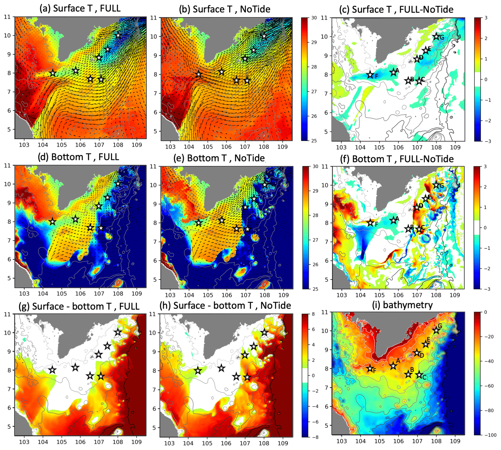
Figure 4 Left and middle columns: surface (a, b) and bottom (d, e) temperature and their differences (g, h) on 16 July 2018 in M17 from the FULL (a, d, g) and NoTide (b, e, h) ensembles [°C]. Arrows show the surface (a, b) or bottom (d, e) horizontal velocity (see Fig. 5 for the values). Right column: (c, f) differences between FULL and NoTide [°C] and (i) bathymetry [m] of the area, with isobaths from 10 to 100 m every 10 m.

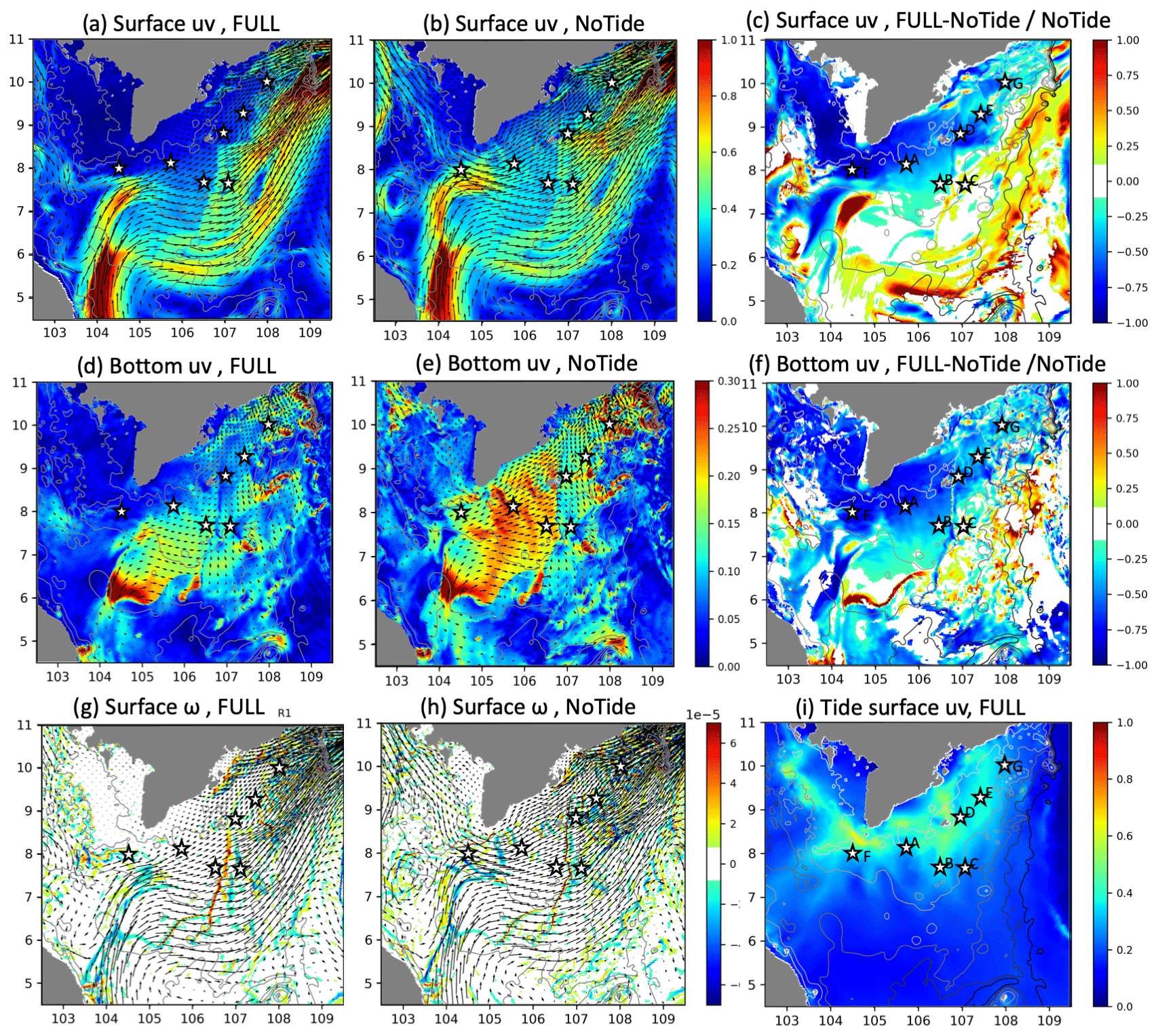
Figure 5 Surface (a, b) and bottom (d, e) horizontal velocity on 16 July 2018 in M17 from the FULL (a, d) and NoTide (b, e) ensembles (in m s⁻¹: colours indicate the speed and arrows the direction). (c, f) Relative differences between FULL and NoTide [no unit]. (g, h) Surface vertical velocity in FULL (g) and NoTide (h) (in m s⁻¹: arrows show the surface horizontal velocity). (i) Surface tidal speed in FULL [m s⁻¹].

In the Gulf of Thailand, a warm surface current (reaching 30 °C) flows southward, following the 40 m isobath (Figs. 4a and 5a). A branch of the Gulf of Thailand current veers east at 8° N around a seamount that rises to 20 m (north of point F; Fig. 4i). Over and north of the mount, the average surface current is extremely weak (less than 5 cm s⁻¹; see the surface velocity maps as well as the profile of horizontal velocity at point F; Figs. 5a and 6f). This horizontal gradient of surface current velocity along the southern flank of the mount results in a divergence associated with positive values of vertical velocity reaching 2 to $\mathrm{5}\times {\mathrm{10}}^{-\mathrm{5}}$ m s⁻¹, i.e. 1 to 4 m d⁻¹ (Fig. 5g). The induced upwelling partly explains the surface cooling observed in this area (SST<28 °C; Fig. 4a).

Figure 6 Profiles of temperature (colour; in °C) and horizontal velocity (arrows; in m s⁻¹) on 16 July and 31 July 2018 at points A, B, C, D, E, and F shown in Figs. 4, 5, and 8 in M17 for the FULL and NoTide ensembles.

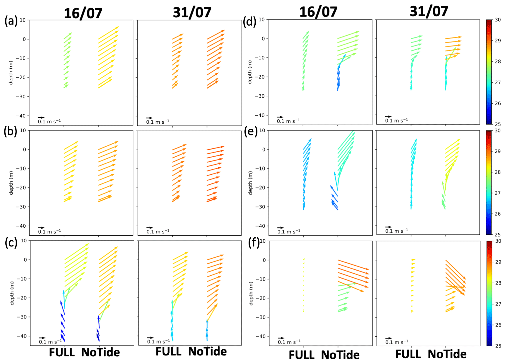
South of the Gulf of Thailand, a northward surface current flows with velocities exceeding 1 m s⁻¹ (Fig. 5a) and relatively cold temperatures compared to the surrounding surface waters (∼28 °C; Fig. 4a). It belongs to the large-scale anticyclonic circulation that prevails in the southeastern SCS. This cold current meets a second branch of the warm southward Gulf of Thailand current, and they both bifurcate northeastward in the area around 4.5–7.5° N, 103.5–105° E. This convergence results in a front of negative surface vertical velocity ($\sim -\mathrm{2}\times {\mathrm{10}}^{-\mathrm{5}}$ m s⁻¹ or $\sim -\mathrm{2}$ m d⁻¹; Fig. 5g), thus resulting in a downwelling of surface water. The downwelled water flows northeastward on the shelf bottom, with velocities reaching 30 cm s⁻¹ (Fig. 5d) and with a temperature of ∼28 °C, much warmer than the surrounding bottom water (<26 °C; Fig. 4d). This area of downwelled water flow corresponds to the area where the difference between the surface and the bottom temperature is negligible (<1 °C; Fig. 4g); i.e. the water column is rather homogeneous. These results are confirmed by the vertically homogeneous profiles of temperature and northeastward horizontal velocity at points A (∼27.5 °C and ∼20 cm s⁻¹; Fig. 6a) and B (∼28.5 °C and ∼30 cm s⁻¹; Fig. 6b), located on the shelf downstream of the area of surface convergence.

Further northeast on the shelf slope, this barotropic warm northeastward current meets a cold bottom northwestward current that flows from the open area towards the coast (Figs. 4d and 5d). At the surface of this bottom convergence, a strong divergence of the northeastward alongshore surface current occurs, with values increasing abruptly from ∼30 to ∼60 cm s⁻¹ (Fig. 5a). This can be seen more quantitatively in the profiles of temperature and velocity at points B and C, located west (upstream) and east (downstream), respectively, of the front of bottom convergence and surface divergence (Fig. 5g). Point C shows a cold (<26 °C) and northwestward current in the bottom layer below 20 m in depth and a warm and fast northeastward current in the surface 0–20 m layer (28.5 °C and ∼50 cm s⁻¹ at the surface; Fig. 6c). This current is almost twice as fast at the surface than the current at point B (∼28.5 °C and ∼30 cm s⁻¹; Fig. 6b), which is northeastward over the entire depth. This bottom convergence of warm northeastward and cold northwestward currents and the divergence of the northeastward surface current are associated with a front of positive vertical velocity between 6 and 8.5° N and 106 and 107° E that reaches $\sim \mathrm{6}\times {\mathrm{10}}^{-\mathrm{5}}$ m s⁻¹ or ∼5 m d⁻¹ (Fig. 5g). The relatively cold bottom water (<27 °C) that results from the meeting of the warm and cold bottom water masses is upwelled and advected northward during this upwelling. It finally emerges at the surface near 8.5° N, where it is advected northeastward by the alongshore current (Figs. 4a and 5a). Points D and E, located further north and downstream of the convergence region, respectively, indeed show homogeneous cold ( 27.5 and <27 °C, respectively) profiles with northeastward velocities (Fig. 6d and e).

The upwelling that develops offshore of the Mekong mouth can therefore be explained by the divergence/convergence associated with gradients of horizontal current resulting from the interactions over marked topography of coastal and offshore surface and bottom circulation that prevails over the area. To further highlight the role of topography, we performed an additional simulation, with the same configuration as member M17 from the FULL ensemble but where we smoothed the topographic anomalies observed along the area of high upward vertical velocity observed in Fig. 5g (Fig. 7a and b). The 10 members of the FULL ensemble as well as the LONG simulation show extremely similar positions and values of strong surface velocity (see Fig. 7c–e, which shows the surface vertical velocity for those simulations on 16 July 2018, the day of MKU intensity peak). In the simulation with smoothed bathymetry, the position of the area of strong vertical surface velocity is modified, shifted by ∼30 km to the west (Fig. 7f). This sensitivity simulation therefore confirms the role of topography in determining the spatial extension of MKU.

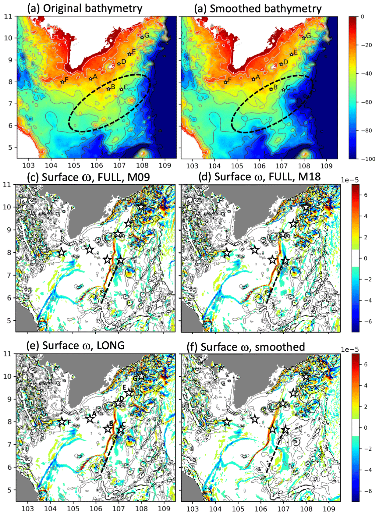
Figure 7 Initial bathymetry (a, in m) and smoothed bathymetry (b); the dashed ellipses show the area of bathymetry smoothing. Surface vertical velocity [m s⁻¹] on 16 July 2018 in M09 (c) and M18 (d) from the FULL ensemble (the other members, not shown, are extremely similar), in LONG (e), and in the sensitivity simulation with smoothed bathymetry (f). The dashed lines in (c)–(f) highlight the front of strong upward vertical velocity.

4.2 Impact of tides

Figure 8 shows the maps of tidal ellipses and currents for the three main tidal components over the MKU region: O₁, K₁, and M₂. It also shows the 0.2 °C isocontour of difference between the JJAS SST in the ensemble averages of FULL and NoTide, corresponding to the area of stronger upwelling southeast of point F and over the eastern slope of the Mekong shelf in FULL compared to in NoTide. Strong tidal currents with velocities reaching 30 cm s⁻¹ for O₁, K₁, and M₂ develop along the southeastern part of the Gulf of Thailand, in the surface convergence area described in Sect. 4.1 (around point F), over the shelf along the Mekong mouth, and over the shelf downstream of the surface divergence area (near points D and E). These areas of strong tidal currents are contiguous with the region of strong JJAS SST difference between FULL and NoTide.

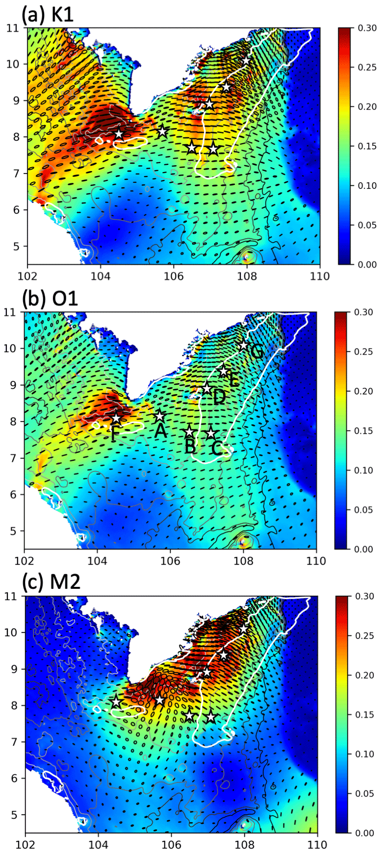
Figure 8 Depth-averaged tidal current ellipses and current intensity [m s⁻¹] in M17 from the FULL ensemble for the three significant tidal components in the MKU region: K₁, O₁, and M₂. The white lines show the 0.2 °C isoline of the difference between JJAS-averaged SST in FULL and in NoTide, corresponding to the area where upwelling is much stronger in FULL than in NoTide in Fig. 1.

We show below that tides actually influence the development of MKU through two mechanisms: their influence on currents and the mixing of cold bottom water with warm waters from shallow areas. Figure 5i shows the tidal surface currents on 16 July 2018 for member M17 of the FULL ensemble. Figure 4b, e, and h shows the surface and bottom temperatures and their difference, and Fig. 5b, e, and h shows the surface and bottom horizontal velocity and the surface vertical velocity for NoTide. Figures 4c and f and 5c and f show the difference in bottom and surface temperature and horizontal velocity between FULL and NoTide.

4.2.1 Tidal influence on the current velocity and its horizontal gradient

The first effect of tides is their impact on the average current. In NoTide, an alongshore coastal current flows over the whole depth, southward in the Gulf of Thailand then northeastward along the Mekong mouth (Fig. 5b and e). In the FULL simulation with tides, this current is non-existent to very weak: its velocity is reduced by more than 75 % (Fig. 5c and f). For points A, B, D, and E, located along this current in NoTide, the velocity decreases from ∼40–50 cm s⁻¹ in NoTide to ∼20 cm s⁻¹ in FULL (Fig. 6a, b, d, and e). For point F, the difference is even stronger, with a 60 cm s⁻¹ surface current in NoTide vs. no current in FULL. The area where the alongshore coastal current is weakened when tides are taken into account (i.e. where the reduction in velocity in FULL compared to NoTide exceeds 50 %; Fig. 5c and f) coincides with the area of strong tidal currents, where the total tidal current reaches an average daily velocity of 50–60 cm s⁻¹ (Fig. 5i). As shown over the Yellow Sea (Moon et al., 2009; Wu et al., 2018; Lin et al., 2022), this weakening of the current flowing over the shallow coastal area is due to the effect of tidal currents that increase the bottom friction and background turbulence due to the nonlinear interaction between wind-driven current and tides in the quadratic bottom friction term (Hunter, 1975).

Conversely, the tide weakly modifies the strong large-scale cyclonic current that originates from the southwest of the domain, with speeds reaching 1 m s⁻¹, and flows northeastward following the shelf slope (Fig. 5a and b). It even slightly increases locally by about ∼20 % (Fig. 5c): the surface velocity downstream of the upwelling front increases from 40 cm s⁻¹ in NoTide to 50 cm s⁻¹ in FULL (Fig. 5a, b and point C; Fig. 6c). The horizontal velocity gradient between the regions of strong northeastward current offshore of the Mekong shelf and of weak current over the shelf is consequently stronger in FULL than in NoTide at both the surface and the bottom (Fig. 5a, b, d, and e). Similarly, the gradient south of the mount near point F strongly increases in FULL. Although they still exist, the surface and bottom convergence and divergence associated with the horizontal velocity gradient upstream and downstream of the Mekong shelf are therefore weakened when tides are removed (Fig. 5h). This first effect of tides on the horizontal velocity gradient thus explains the weakening of the associated downwelling and upwelling in NoTide compared to FULL.

4.2.2 Effect of tidal mixing on vertical stratification

The second contribution of tides to the upwelling is related to the tidally induced vertical mixing of water masses. This tidal mixing contributes to the homogenization of the water column and to the surface cooling, thus enhancing the effect of the horizontal gradient of surface and bottom currents described above. This effect occurs in specific areas of the domain upstream and downstream of the Mekong shelf. For FULL and NoTide, Fig. 9 shows the profiles of temperature and vertical diffusivity for points A to F, k_z, quantifying the vertical mixing. Points D, E, and F are located in the area of strong tidal currents (Fig. 8) upstream of the surface convergence zone (point F; Fig. 5g) and downstream of the surface divergence zone (points D and E). For those points, k_z is much stronger in FULL ($>{\mathrm{10}}^{-\mathrm{2}}$ m² s⁻¹) than in NoTide (between 10⁻⁵ and 10⁻² m² s⁻¹; Fig. 9b). As a result, the temperature is vertically homogeneous in FULL, whereas NoTide shows a strong vertical temperature gradient of 1 to 2 °C and warmer surface water and colder bottom water compared to FULL (Fig. 9a). Tidal mixing thus significantly contributes to the upwelling there. Conversely, for points A and B located on the Mekong shelf, the temperature is vertically homogeneous (although slightly warmer in NoTide compared to FULL, by ∼0.5 °C) and k_z is similar (between 10⁻² and 10⁻¹ m² s⁻¹) in both simulations. The low stratification in the shelf region between the surface convergence and divergence areas is thus not due to a local effect of vertical tidal mixing over the shelf itself. It rather results from the advection by the northeastward current of the water downwelled and mixed by tides remotely, upstream of the shelf. Besides vertical mixing, lateral mixing induced by bottom tidal currents explains the eastward intrusion of cold, deep water over the western bottom shelf slope near 104° E (Fig. 4f). This cold water is then advected over the shelf by the alongshore current, thus also contributing to the water cooling in the downstream area.

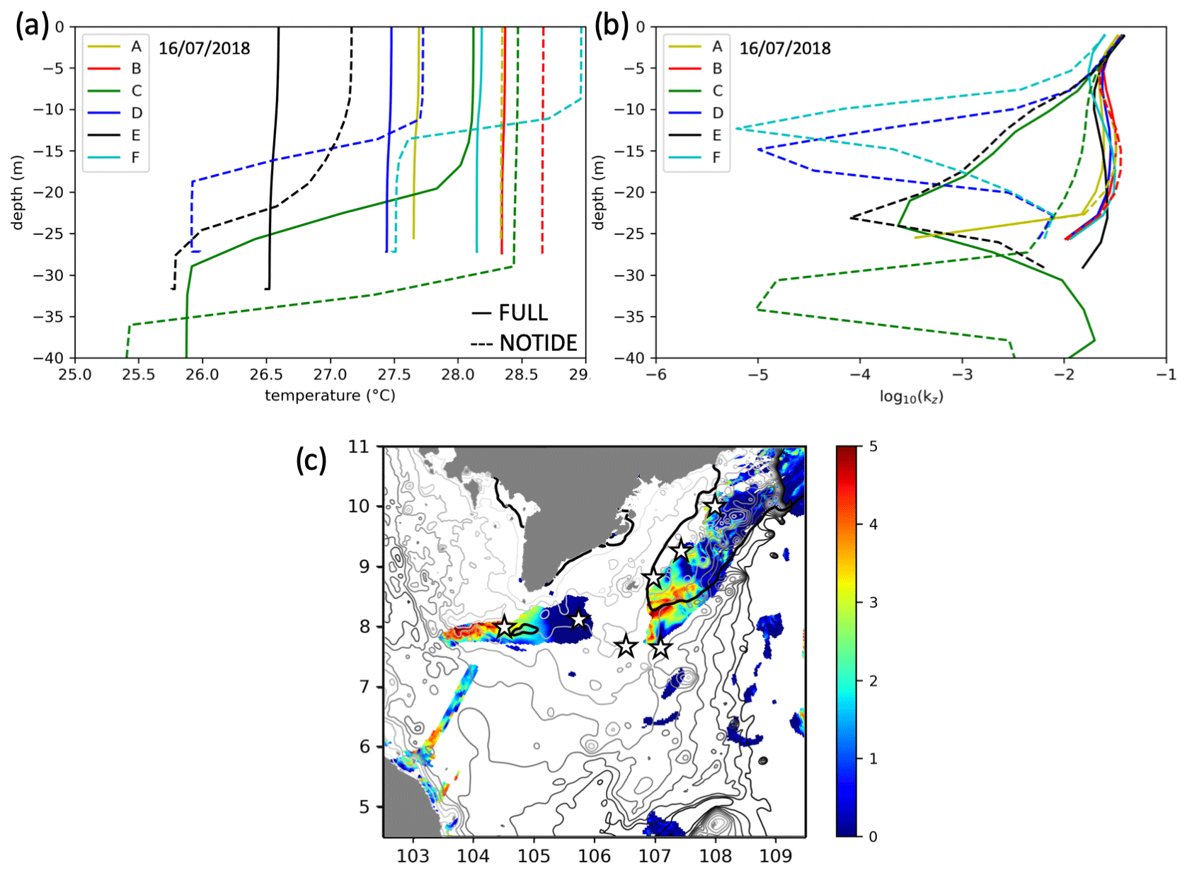
Figure 9 Profiles of temperature (a; in °C) and diffusivity coefficient k_z (b; in m² s⁻¹, logarithmic scale) on 16 July 2018 at points A, B, C, D, E, and F shown in Figs. 4, 5, and 8 in M17 from the FULL (solid lines) and NoTide (dashed line) ensembles. (c) Map of the maximum over the water column of the difference in diffusivity coefficient between FULL and NoTide, Δlog ₁₀(k_z), from the same day as (b), plotted for areas where the FULL − NoTide SST difference exceeds 0.4 °C. The black line shows the T_o=27.6 °C surface isotherm.

This effect of tidal mixing allows MKU to be partially maintained during the midsummer low-wind period (late July–early August; Fig. 3a and h). During this period, MKU indeed reaches a local minimum in the FULL ensemble, whereas it completely disappears in the NoTide ensemble. Figure 6 shows the vertical profiles of temperature and horizontal currents for points A–F in FULL and NoTide on 31 July, i.e. the day of minimum wind and UI_d,boxMK during this low-wind period. Over the shelf, the velocity of the northeastward surface current as well its gradient are reduced on 31 July compared to 16 July in both FULL and NoTide. In NoTide, velocity is about 40 cm s⁻¹ at A, B, and C on 16 July and about 30 cm s⁻¹ on 31 July, with negligible velocity difference between these points. The upwelling completely vanishes. In FULL, velocity on 31 July goes from ∼20 cm s⁻¹ at A to ∼30 cm s⁻¹ at B and C vs. 20, 30 and 50 cm s⁻¹, respectively, on 16 July. The difference between C and A thus decreases from ∼30 cm s⁻¹ on 16 July to ∼10 cm s⁻¹ on 31 July. This strongly reduces the upwelling due to the horizontal velocity gradient effect in FULL. Besides, points E and F (and to a lower extent point D) still show fully homogeneous temperature profiles in FULL on 31 July vs. stratified profiles in NoTide, with ∼0.5 and 1 °C temperature differences between the surface and bottom, respectively. Tidal mixing therefore still occurs in FULL, inducing partial surface cooling and contributing to the maintenance of MKU. During the period of low wind, the contribution of the horizontal circulation gradient to MKU is therefore strongly weakened, and tidal mixing is a major factor in maintaining MKU.

Tidal mixing therefore enhances the upwelling through both a local effect (direct mixing of water column) and a remote effect (advection of water mixed upstream). These effects are eventually transmitted to SCU through the advection of water upwelled in MKU to the SCU zone. This explains the significantly higher UI_d for SCU during the midsummer low-wind period (∼20 %; Fig. 3b).

To quantify the respective contributions of local and remote effects to the surface cooling, we examine the maximum of the difference in vertical diffusivity coefficient k_zover the water column between FULL and NoTide, Δlog ₁₀(k_z). Figure 9c shows the map of Δlog ₁₀(Kz) together with the −0.4 °C contours of the SST difference between FULL and NoTide, which highlights the area of surface cooling induced by tides, and the T_o isotherm in FULL, which highlights the area of upwelling. A value of Δlog ₁₀(Kz) higher than 2 means that the vertical mixing induced locally by tides dominates the vertical mixing, i.e. upstream of the Mekong shelf (point F) and in the wake of Con Day island (points D and E; see profiles of temperature and k_z in Fig. 9a and b). A value lower than 1 means that tides do not significantly contribute to the local vertical mixing, i.e. over the Mekong shelf between the surface convergence and divergence zones (point A downstream of point F).

4.3 Effect of rivers

The NoRiver ensemble produces a slightly higher MKU than FULL, with the strongest difference (∼30 %) in the UI_d,boxMK ensemble average on 31 July during the midsummer low-wind period (Fig. 3h) and a 9 % increase in UI_JJAS,boxMK (Table 1). Figure 10a and b shows the maps of the difference in sea surface salinity (SSS) and temperature (SST) between NoRiver and FULL on 31 July. Removing Mekong River discharge logically results in a strong increase in sea surface salinity near the Mekong mouth in NoRiver compared to FULL. The area of ∼1 psu SSS difference highlights the Mekong plume, which is removed in NoRiver. The upwelling intensification in NoRiver occurs in the northeastern part of this plume, with a ∼1 °C SST cooling compared to FULL (point G; Fig. 10b).

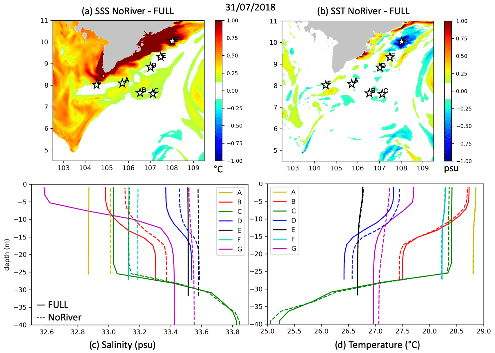
Figure 10 (a, b) Difference in sea surface salinity (a; in psu) and temperature (b; in °C) between M17 from the NoRiver and FULL ensembles over the MKU region on 31 July 2018. (c, d) Corresponding profiles of salinity (c) and temperature (d) over points A–G shown in panels (a) and (b) for the FULL (solid lines) and NoTide (dashed line) ensembles.

This removal of the upper layer of fresher and hence lighter water in NoRiver induces a weakening of the vertical stratification. Figure 10c and d shows the vertical profiles of salinity and temperature for points A–G on 31 July in both simulations. For points A to F, located south of the Mekong plume, temperature and salinity vertical profiles are very similar in NoRiver and FULL, even if slightly shifted. More specifically, the vertical gradients of temperature and salinity are similar in both simulations: differences in the surface–bottom difference between NoRiver and FULL are smaller than 0.1 °C and 0.1 psu. For those points, the stratification is therefore not significantly modified by river discharge. Conversely, for point G, located in the MKU area downstream of point E but also in the Mekong plume area (Fig. 10a), those profiles are very different in NoRiver and FULL. The salinity difference between the surface and the bottom is ∼1 psu in FULL vs. less than 0.1 psu in NoRiver, and the temperature difference is 0.6 °C in FULL vs. 0.1 °C in NoRiver. The stratification at point G is therefore significantly weakened in NoRiver. This stratification weakening makes the water column easier to mix vertically, facilitating the tidal vertical mixing that is the main contributor to MKU in this area and during the transition period, as explained above. The resulting surface cooling finally explains the increase in MKU intensity in NoRiver. Rivers thus locally hinder the development of MKU through their strengthening effect on the stratification.

This area of Mekong plume influence on the stratification and on MKU is, however, small, as highlighted by Fig. 10a and c (limited to point G) and confirmed by Fig. 2: in the area where upwelling develops, the sea surface salinity difference between FULL and NoRiver does not exceed 1.0 psu. The area where strong buoyancy gradients can develop and enhance chaotic variability therefore does not reach the MKU region, explaining the non-significant effect of river discharge on MKU OIV (Fig. 3i). The JJAS SST difference between FULL and NoRiver moreover shows that the river effect on the stratification is not sufficient to significantly enhance the Ekman-transport-driven upwelling at the coast (Fig. 1f).

5 Representativeness of summer 2018

Wind and upwelling intensity over the SVU region were stronger than average during summer 2018 and weaker during summer 2017 (To Duy et al., 2022). To discuss the representativeness of the results and conclusions obtained from the analysis of summer 2018, we thus examine the spatial and temporal variability in upwelling for summer 2017 in the FULL, NoTide, and NoRiver 2-year ensembles. Figure 11 shows the maps of summer SST in the three ensembles for 2017, and Fig. 12 shows the daily time series of wind and upwelling indicators.

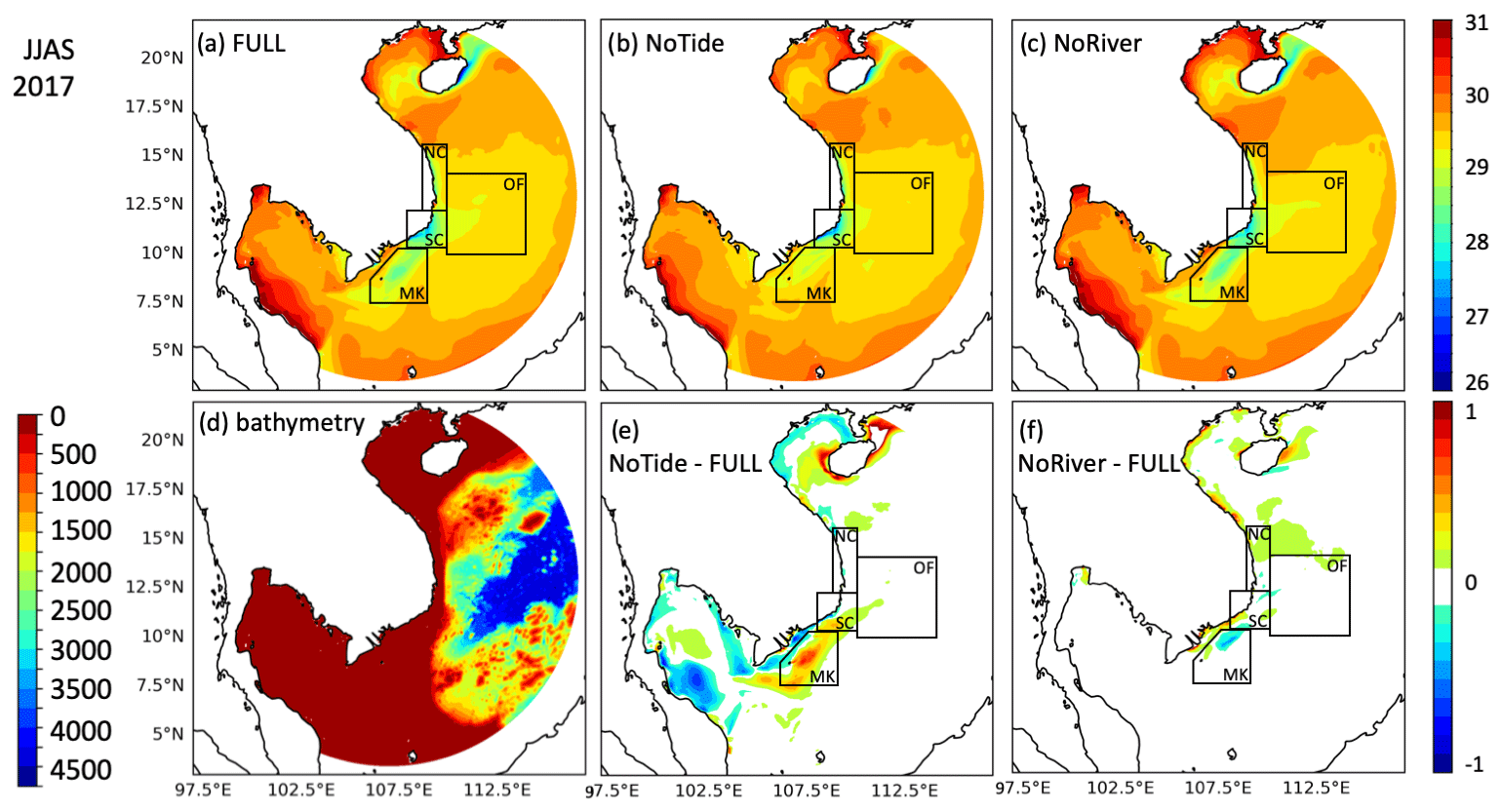
Figure 11 Same as Fig. 1 but for summer 2017.

The analysis of summer 2017 is in agreement with the analysis of summer 2018. First, the intraseasonal chronology of OFU, SCU, and MKU intensity is primarily driven by wind (Fig. 12a, b, d, and h, with highly significant correlations between 0.55 and 0.68, p value<0.01 between UI_d,B and wind for both summers). It is not the case for the intraseasonal chronology of NCU (Fig. 12a and f) that only develops at the beginning and end of summer 2017, confirming our conclusion about the blocking role of the core of summer general circulation. Second, the influence of OIV on upwelling intensity is very weak for MKU, weak for SCU, and stronger for OFU and NCU (Fig. 12c, e, g, and i). Third, tides have a major role in MKU development in both 2017 and 2018, with no MKU developing at all in the NoTide ensemble in summer 2017 (Figs. 11e and 12h). Rivers slightly reduce MKU intensity in the middle of summer, whereas neither tides nor rivers significantly impact the upwelling over the other three areas (Figs. 11e, f and 12b–h).

Figure 12 Same as Fig. 3 but for summer 2017.

To complete this analysis, we examine the summer upwelling location for different years/members in Fig. 2. For the 10 members of the FULL ensemble, MKU rigorously shows the same location of development for summer 2018 and is similar for summer 2017, although its extension is strongly reduced. Between 2009 and 2018 in the LONG simulation, MKU also always develops over the same core area, with a spatial extension varying with the strength of the upwelling. Those results, together with the sensitivity analysis to topography (Sect. 4.1), confirm the stability of MKU location related to the influence of topography.

6 Conclusions

We studied here the effect of tides and rivers on the intensity of SVU over its four areas of development at the daily to intraseasonal scale and explored the detailed mechanisms explaining the development of upwelling over the Mekong shelf, MKU. For that, a reference and two sensitivity ensembles of 10 members were performed for the case study of the strong upwelling that occurred during summer 2018 along and offshore of the Vietnamese coast.

Tides contribute strongly to MKU intensity, increasing its summer average by a factor of 3.5, whereas rivers slightly reduce it, by 9 % of the summer average. Tides slightly increase SCU intensity during the midsummer low-wind period, and rivers do not affect it. Tides and rivers do not have a statistically significant influence on the upwelling in the offshore and northern coastal regions, OFU and NCU. For the four upwelling areas, neither tides nor rivers significantly influence the upwelling intraseasonal chronology. For OFU, SCU, and MKU, wind therefore remains the main driver of the upwelling chronology, whereas for NCU, the effect of large-scale circulation predominates.

Circulation and tides interacting over marked topography are the main factors that explain MKU development. The interactions of a weak coastal alongshore shallow current flowing over the Mekong shelf and strong surface and bottom currents that prevail offshore around the shelf locally induce strong convergence or divergence of horizontal currents on the western and eastern flanks of the shelf slope. This results in high vertical velocities (on the order of a few metres per day), with a downwelling upstream (west) of the shelf and an upwelling downstream (east) of the shelf. Tidal currents first enhance the bottom friction and background turbulence, which weaken the coastal alongshore shallow current. This increases the horizontal velocity gradient, the resulting divergence and convergence, and associated vertical velocities, hence intensifying the induced downwelling and upwelling. Second, tides contribute to the vertical and lateral mixing of cold bottom waters with shallower warmer water. The advection into the upwelling region of the resulting cold water masses further intensifies the surface cooling. This effect of tidal mixing explains most of the MKU maintenance during the low-wind midsummer period, during which time the circulation mechanisms barely induce the upwelling. The water upwelled in the MKU area is moreover advected into the SCU area, explaining the ∼20 % contribution of tides to SCU intensity during this period. Last, surface freshwater from the Mekong River slightly weakens the MKU intensity (by up to 30 % during the low-wind period) by strengthening the vertical stratification. MKU is therefore mostly driven by non-chaotic processes (large-scale circulation, topography, and tides), which explains its negligible OIV compared to NCU and OFU. A further analysis of the summers of 2009 to 2017 suggests that those conclusions are robust throughout the different years and associated atmospheric, oceanic, and river conditions. Figure 13 summarizes these findings on the processes involved in the functioning of MKU.

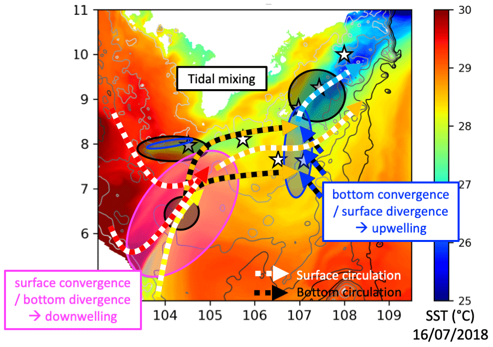
Figure 13 Schematic representation of MKU functioning. Arrows represent the surface (white) and bottom (black) circulation and the associated temperatures (colours).

Following and complementing the previous studies about the SVU, this study allowed us to deepen our understanding of the physical mechanisms involved in the functioning of and variability in this upwelling over its different areas of development: wind, (sub-)mesoscale dynamics, ocean intrinsic variability, tides, rivers, and topography. New studies are now required to better understand the influence of the upwelling on the planktonic ecosystems, notably based on the use of coupled physical–biogeochemical modelling (e.g. SYMPHONIE-Eco3M-S; Ulses et al., 2016; Herrmann et al., 2017). The surface cooling associated with the SVU and its different mechanisms is moreover part of the heat budget of the regional climate system. Several studies also highlighted the impact of the SVU on local atmospheric dynamics, including winds (Zheng et al., 2016; Yu et al., 2020). Using online closed budget tools, as was done by Trinh et al. (2024) over the whole South China Sea, as well as ocean–atmosphere coupled models such as the SYMPHONIE-RegCM recently developed by Desmet (2024) will now allow us to better understand and quantify the role of the upwelling as well as other factors in those budgets, its feedback into the atmospheric dynamics and local climate, and its response to climate change, especially since climate projections predict a weakening of the summer winds (Herrmann et al., 2020, 2021). Applying perturbations to the atmospheric fields that drive the upwelling (i.e. the wind; see for example Nguyen-Duy et al., 2023) or to the lateral boundary conditions that would create a different sub-mesoscale to mesoscale circulation (i.e. the wind; see for example Da et al., 2019) would also introduce chaos into our simulations and would be interesting to study. Beside these modelling efforts, dedicated in situ campaigns would be extremely useful to confirm our conclusions, in particular for MKU for which extremely little data are available.