Extension of Ekman (1905) wind-driven transport theory to the β plane

The seminal Ekman (1905) f-plane theory of wind-driven transport at the ocean surface is extended to the β plane by substituting the pseudo-angular momentum for the zonal velocity in the Lagrangian equation. When the β term is added, the equations become nonlinear, which greatly complicates the analysis. Though rotation relates the momentum equations in the zonal and the meridional directions, the transformation to pseudo-angular momentum greatly simplifies the longitudinal dynamics, which yields a clear description of the meridional dynamics in terms of a slow drift compounded by fast oscillations; this can then be applied to describe the motion in the zonal direction. Both analytical expressions and numerical calculations highlight the critical role of the Equator in determining the trajectories of water columns forced by eastward-directed (in the Northern Hemisphere) wind stress even when the water columns are initiated far from the Equator. Our results demonstrate that the averaged motion in the zonal direction depends on the amplitude of the meridional oscillations and is independent of the direction of the wind stress. The zonal drift is determined by a balance between the initial conditions and the magnitude of the wind stress, so it can be as large as the mean meridional motion; i.e., the averaged flow direction is not necessarily perpendicular to the wind direction.

1 Introduction

The seminal theory of wind-driven transport at the ocean surface was developed about 120 years ago by the Swedish oceanographer Vagn Walfrid Ekman for the highly idealized case of constant Coriolis frequency – the f plane. The Ekman (1905) theory addresses the downward-spiraling horizontal velocity in the ocean's surface and its vertical integral – the transport. Ekman's elegant solution of the problem has become textbook material in physical oceanography, dynamical meteorology, and geophysical fluid dynamics (see, e.g., Gill, 1982; Pedlosky, 1987; Vallis, 2017). For uniform wind stress the dynamics on the f plane consist of two parts: a steady flow to the right and left of the wind direction in the Northern and Southern Hemisphere and inertial oscillations (of frequency f₀ – the constant Coriolis frequency). However, though it is one of the cornerstones of atmosphere and ocean dynamics, the theory was never extended to include the latitudinal increase in the Coriolis frequency, known as the β effect, which is the focus of the present study. In contrast to the β plane, in spherical coordinates the theory of wind-driven transport was studied numerically in Constantin and Johnson (2019) and Paldor (2002), but due to the complexity of the governing equations in these coordinates, the numerical solutions have not yielded analytic understanding. With the wind-driven dynamics on the f plane fully understood and quantified, the β plane offers an in-between set-up wherein analytical insight can complement the numerical solutions.

For given wind stress forcing, the known general differences between the dynamics on the f plane and β plane heuristically suggest that the extension of Ekman's transport theory to the β plane should include the following qualitative elements.

1. An increase or decrease in mean meridional velocity for an eastward- or westward-directed stress due to the decrease or increase in Coriolis frequency when the water column moves southward or northward.

2. The frequency of oscillation about the mean velocity should decrease or increase (so oscillation period should increase or decrease) due to the decrease or increase in Coriolis frequency along the trajectory (for an eastward-directed stress in the Northern Hemisphere, while the opposite changes occur for westward-directed stress and in the Southern Hemisphere).

3. Since the oscillation's frequency and amplitude are inversely correlated (energy flux is unchanged) a decrease in frequency should lead to an increase in amplitude and vise versa.

4. Since inertial oscillations that form a perfectly circular motion on the f plane drift westward on the β plane, the averaged zonal motion should drift to the west. A heuristic reasoning of the westward drift in terms of the change in the radius of the inertia circle was proposed by Von Arx (1964), and complete quantitative theories of the drift were developed in Ripa (1997) and Paldor (2007).

The numerical solutions of the governing Lagrangian equations (see Sect. 2 below) shown in Fig. 1 fully confirm the first three expectations listed above but contradict the fourth one – for both westward (right panel) and eastward (left panel) stresses, the trajectories drift to the east. From the particular example shown in Fig. 1 it is unclear whether the eastward transition is a general feature of the wind-driven dynamics on the β plane or a specific occurrence related to the particular choice of initial conditions and/or parameter values.

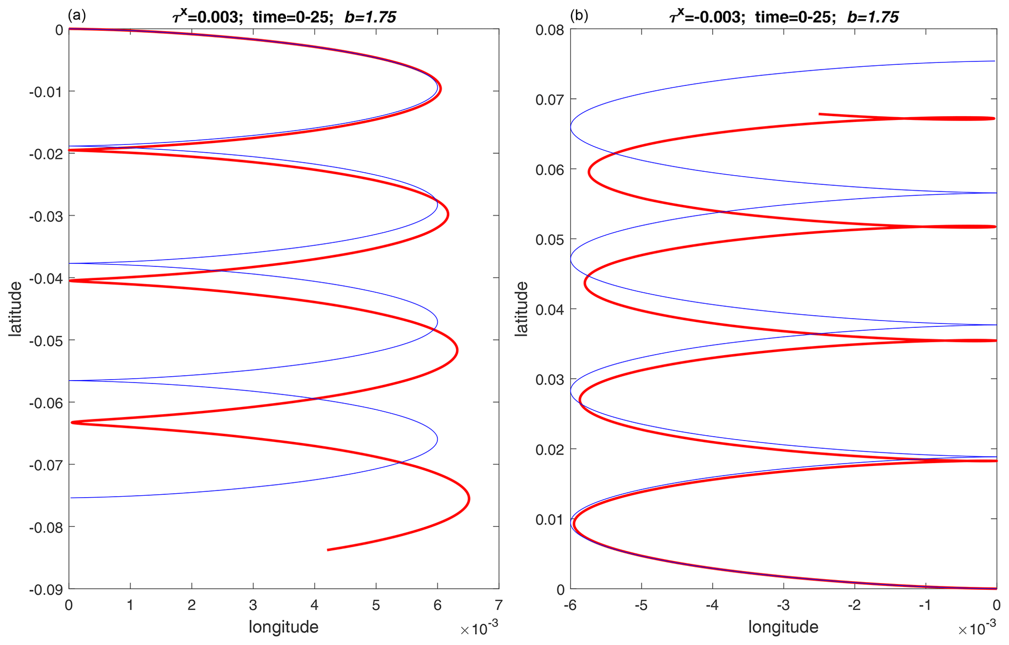
Figure 1 The (longitude, latitude) trajectories of water columns at the ocean surface subject to westward-directed (b) and eastward-directed (a) wind stress on the f plane (blue curves) and on the β plane (red curves). The time unit is the inverse of the mean Coriolis frequency, and the longitude and latitude distances are scaled on Earth's radius. The value of b (scaled β) corresponds to 30^∘ latitude. The scaling of the wind stress (τ^x) is detailed in Sect. 2. Both trajectories start from $(x,y)=(\mathrm{0},\mathrm{0})$ located at the bottom right point in the right panel and at the upper left point in the left panel.

In addition to resolving the issue of the zonal drift and quantifying the various rates of changes, the present study also addresses the equatorial problem that exists only on the β plane. This equatorial issue can be described as follows: an eastward-directed stress in the Northern Hemisphere forces a net southward-directed mean flow, which, on the β plane, is accompanied by a decrease in the Coriolis frequency. Thus, at some time the wind-forced water column must find itself at a latitude at which the Coriolis frequency vanishes – the Equator. From that point onward the water column is subject to non-rotating dynamics and must move eastward at an accelerated velocity. In the rest of this work we will estimate the time it takes the water column to change its dynamics from rotating to non-rotating and analyze how the two dynamical regimes connect with one another.

The work is organized as follows: in Sect. 2 we nondimensionalize the governing Lagrangian equations and simplify them by substituting the pseudo-angular momentum for the zonal velocity. The simplified system is analyzed in Sect. 3, and the work concludes with a discussion and summary in Sect. 4.

2 The nondimensional model

The time-dependent trajectory of a column of water in the surface Ekman layer forced by the overlying uniform wind stress on the f plane is a fundamental problem of physical oceanography that is fully described in most textbooks (Gill, 1982; Pedlosky, 1987; Vallis, 2017). The governing Lagrangian equations that describe the dynamics of vertically averaged horizontal velocity components consist of the momentum equations in the zonal and meridional directions and the (trivial) relations between these velocity components as well as the changes in the coordinate of the moving column, i.e.,

$$\begin{array}{}\text{(1)}& {\displaystyle \frac{\mathrm{d}x}{\mathrm{d}t}}=U,{\displaystyle \frac{\mathrm{d}y}{\mathrm{d}t}}=V,{\displaystyle \frac{\mathrm{d}U}{\mathrm{d}t}}=fV+{\displaystyle \frac{{\mathit{\tau }}^x}{H\mathit{\rho }}},{\displaystyle \frac{\mathrm{d}V}{\mathrm{d}t}}=-fU.\end{array}$$

Here τ^x is the uniform zonally directed wind stress (which is positive or negative for eastward- or westward-directed wind, respectively), ρ is the water density, H is the depth (thickness) of the layer, $f=f_{\mathrm{0}}+\mathit{\beta }y$ is the Coriolis parameter (where f₀=2Ωsin(ϕ₀), β=2Ωcos(ϕ₀) $/$ R_e with R_e and Ω – Earth's radius and rotation frequency, respectively, and ϕ₀ – the latitude at which the plane is tangential to Earth), U and V are the vertically averaged horizontal velocity components in the eastward and northward directions, respectively, and x and y are the respective coordinates in these directions. The only added complication of this system relative to that studied in detail in, e.g., Ch. 9 of Gill (1982), is that here the Coriolis frequency, f, in the momentum equations is y-dependent.

The four-dimensional system (Eq. 1) can be easily integrated numerically, but the general properties of its solutions can be best deciphered by reducing the number of its free parameters. This is done by scaling time, t, on $\frac{\mathrm{1}}{f_{\mathrm{0}}}$ and x and y on R_e so the velocity scale is f₀R_e. With this scaling the nondimensional Coriolis frequency is 1+by, where $b=\frac{\mathit{\beta }{R}_{\mathrm{e}}}{f_{\mathrm{0}}}=\text{cot}\left({\mathit{\varphi }}_{\mathrm{0}}\right)$ is the nondimensional β. The system is further simplified by replacing U by the pseudo-angular momentum, defined as $D=U-y(\mathrm{1}+\frac{b}{\mathrm{2}}y)$ in nondimensional units. As was shown by Paldor (2007), when τ^x=0, i.e., in the inertial case, D is conserved. We note that in spherical coordinates the conservation of angular momentum, which is the spherical counterpart of D, yields a simple relation between the zonal velocity and the latitude (Paldor, 2001). Formally, a similar quantity relating the zonal velocity, U, and the meridional coordinate, y, can also be derived in Cartesian coordinates, but, unlike spherical coordinates, this conserved quantity is not the angular momentum. With these changes the system (Eq. 1) transforms to

$$\begin{array}{}\text{(2)}& {\displaystyle \frac{\mathrm{d}x}{\mathrm{d}t}}=D+y\left(\mathrm{1}+{\displaystyle \frac{b}{\mathrm{2}}}y\right),\text{(3)}& {\displaystyle \frac{\mathrm{d}y}{\mathrm{d}t}}=V,\text{(4)}& {\displaystyle \frac{\mathrm{d}D}{\mathrm{d}t}}=\mathrm{\Gamma },\text{(5)}& {\displaystyle \frac{\mathrm{d}V}{\mathrm{d}t}}=-(\mathrm{1}+by)\left(D+y\left(\mathrm{1}+{\displaystyle \frac{b}{\mathrm{2}}}y\right)\right).\end{array}$$

Here t, x, y, and V denote the nondimensional counterparts of the dimensional variables denoted by the same symbols in Eq. (1), and, as explained above, $D=U-y(\mathrm{1}+\frac{b}{\mathrm{2}}y)$ is the nondimensional pseudo-angular momentum. Equation (4) confirms that D is indeed conserved when Γ=0. The solutions of this system are determined by the four required initial conditions and the two parameters $b=\frac{\mathit{\beta }{R}_{\mathrm{e}}}{f_{\mathrm{0}}}=$ cot(ϕ₀), the nondimensional β, and $\mathrm{\Gamma }=\frac{{\mathit{\tau }}^x}{H\mathit{\rho }{f}_{\mathrm{0}}^{\mathrm{2}}{R}_{\mathrm{e}}}$, the constant nondimensional surface wind stress. The value of b at ${\mathit{\varphi }}_{\mathrm{0}}=\mathrm{30}{}^{\circ }$ is 1.75. For realistic values (${\mathit{\tau }}^x/\mathit{\rho }\approx \mathrm{2}\times {\mathrm{10}}^{-\mathrm{4}}$ m² s⁻², $f_{\mathrm{0}}={\mathrm{10}}^{-\mathrm{4}}$ s⁻¹, and H=30 m), the value of $\mathrm{\Gamma }={\mathrm{10}}^{-\mathrm{3}}$, so the theory should be applicable to b of O(1) and Γ≪1. The sign of Γ is that of τ^x – positive for eastward-directed stress and negative for westward-directed stress.

We solve this system by starting at the origin of the β plane, i.e., $x\left(\mathrm{0}\right)=y\left(\mathrm{0}\right)=\mathrm{0}$, and assume that the initial V(0) and D(0)=U(0) are sufficiently small. The numerical solutions presented below are initiated with D(0)=0 and V(0)≠0. However, the definition of D implies that trajectories emanating from D(0)≠0 and y(0)=0 can also be calculated starting from D(0)=0 and a suitable y(0)≠0. Note that the choice D(0)=0 does not restrict the generality of our solutions since the shift of time from t to $t^{\prime }=t+D\left(\mathrm{0}\right)/\mathrm{\Gamma }$ yields $D(t^{\prime }=\mathrm{0})=\mathrm{0}$, so D(0)=0 can be assumed. The analysis of the solutions of Eqs. (2)–(5), including numerical examples, are presented in the next section.

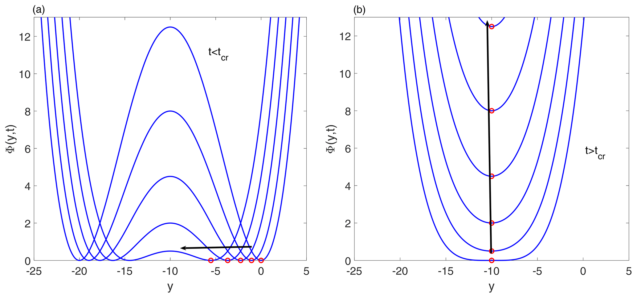
Figure 2 A schematic demonstration of the change in the potential Φ(y,t) for b=0.1 and Γ=0.1 at $t=\mathrm{0},\mathrm{10},\mathrm{20},\mathrm{\dots },\mathrm{100}$. The direction of increase in time is indicated by the black arrows for t<t_cr (a) and t>t_cr (b). The minima, $y_{\mathrm{m}}^{+}$, of the potentials are indicted by red circles.

3 Analysis

The analysis of Eqs. (2)–(5) begins with the (V, y) subsystem, i.e., Eqs. (3) and (5) along with the (trivial) solution D=Γt of Eq. (4). The derived solution of y(t) will then be substituted in Eq. (2) to yield the zonal propagation speed. First, we combine Eqs. (3) and (5) to the single second-order equation

$$\begin{array}{}\text{(6)}& {\displaystyle \frac{d^{\mathrm{2}}y}{\mathrm{d}{t}^{\mathrm{2}}}}=-(\mathrm{1}+by)\left[D+y\left(\mathrm{1}+{\displaystyle \frac{b}{\mathrm{2}}}y\right)\right].\end{array}$$

We will discuss solutions of this equation for initial conditions in the vicinity of $y=\mathrm{d}y/\mathrm{d}t=V=\mathrm{0}$ and assume that Γ is sufficiently small (for the smallness condition see Eq. A3 in the Appendix). We proceed by rewriting Eq. (6) as

$$\begin{array}{}\text{(7)}& {\displaystyle \frac{d^{\mathrm{2}}y}{\mathrm{d}{t}^{\mathrm{2}}}}=-{\displaystyle \frac{\partial \mathrm{\Phi }(y,t)}{\partial y}},\end{array}$$

where

$$\begin{array}{}\text{(8)}& \mathrm{\Phi }(y,t)={\displaystyle \frac{\mathrm{1}}{\mathrm{2}}}{\left[\mathrm{\Gamma }t+y\left(\mathrm{1}+{\displaystyle \frac{\mathrm{1}}{\mathrm{2}}}by\right)\right]}^{\mathrm{2}}.\end{array}$$

Equation (7) describes the dynamics of a quasi-particle in a slowly (for small Γ) time-varying quasi-potential well Φ(y,t). In Fig. 2 we illustrate this potential for $\mathrm{\Gamma }=b=\mathrm{0.1}$ at times $t=\mathrm{0},\mathrm{10},\mathrm{20},\mathrm{\dots },\mathrm{100}$. The minima of these potentials, denoted collectively by y_m, are given by the three roots of

$$\begin{array}{}\text{(9)}& {\displaystyle \frac{\partial \mathrm{\Phi }}{\partial y}}{|}_{y=y_{\mathrm{m}}}=\left[\mathrm{\Gamma }t+y_{\mathrm{m}}\left(\mathrm{1}+{\displaystyle \frac{\mathrm{1}}{\mathrm{2}}}b{y}_{\mathrm{m}}\right)\right](\mathrm{1}+b{y}_{\mathrm{m}})=\mathrm{0}.\end{array}$$

Two cases should be considered depending on time being below or above the critical time

$$\begin{array}{}\text{(10)}& t_{\mathrm{cr}}={\displaystyle \frac{\mathrm{1}}{\mathrm{2}b\mathrm{\Gamma }}}.\end{array}$$

For t<t_cr, there are two minima defined by $\mathrm{\Gamma }t+y_{\mathrm{m}}\left(\mathrm{1}+\frac{\mathrm{1}}{\mathrm{2}}b{y}_{\mathrm{m}}\right)=\mathrm{0}$, i.e.,

$$\begin{array}{}\text{(11)}& y_{\mathrm{m}}^{\pm }={\displaystyle \frac{\mathrm{1}}{b}}(-\mathrm{1}\pm \sqrt{\mathrm{1}-\mathrm{2}b\mathrm{\Gamma }t}),\end{array}$$

while for t>t_cr, there is a single minimum located at

$$\begin{array}{}\text{(12)}& y_{\mathrm{m}}^{\mathrm{0}}=-{\displaystyle \frac{\mathrm{1}}{b}}.\end{array}$$

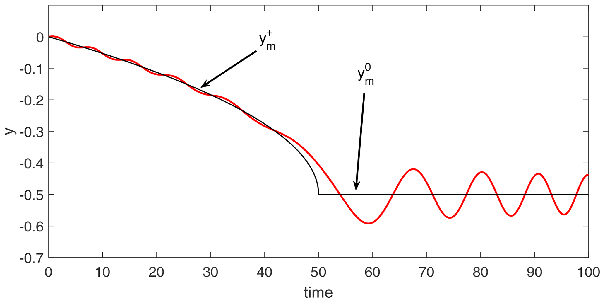
Figure 3 shows the numerical solutions of y(t) when the column originates near $y_{\mathrm{m}}^{+}$; i.e., $x=y=D=\mathrm{0}$ and V=0.002. As predicted, the exact solution of y(t) oscillates with small amplitude (that increases with the value of V(t=0)) about the evolution curves of $y_{\mathrm{m}}^{+}$ and $y_{\mathrm{m}}^{\mathrm{0}}$ shown by the black curves. The direction of evolution of $y_{\mathrm{m}}^{+}\left(t\right)$ and its transformation to the constant $y_{\mathrm{m}}^{\mathrm{0}}\left(t\right)$ at t=t_cr correspond to the evolution of the red circles in Fig. 2 for t<t_cr (a) and t>t_cr (b). The averaged numerical solution is expected to deviate appreciably from the simple scenario shown here only for high oscillation amplitude near $y_{\mathrm{m}}^{+}$.

The main idea of the following analysis is that since the system starts near $y=\mathrm{d}y/\mathrm{d}t=V=\mathrm{0}$, i.e., near the minimum of the potential, $y_{\mathrm{m}}^{+}$, by the adiabatic theory (see pages 531–535 in Goldstein, 1980), it will stay near this minimum for t<t_cr. At t=t_cr, $y_{\mathrm{m}}^{+}$ transforms into $y_{\mathrm{m}}^{\mathrm{0}}$, and therefore at all t>t_cr, the system remains near $y_{\mathrm{m}}^{\mathrm{0}}$. Thus, the column remains near the minimum of Φ at all times, while this minimum slowly decreases for t<t_cr and stays constant for t>t_cr. Since the trajectory originates near the minimum $y_{\mathrm{m}}^{+}$ and since for small Γ the variation of the potential is slow (see Eq. 9), we expect the solution for y to be of the form

$$\begin{array}{}\text{(13)}& y=y_{\mathrm{m}}\left(t\right)+\mathit{\delta }y,\end{array}$$

where y_m(t) starts at $y_{\mathrm{m}}^{+}$ and later (i.e., at t=t_cr) transforms into $y_{\mathrm{m}}^{\mathrm{0}}$, and δy is a small perturbation. We substitute this form of solution into Eq. (6) and rewrite the resulting equation as

$$\begin{array}{}\text{(14)}& {\displaystyle \frac{d^{\mathrm{2}}\mathit{\delta }y}{\mathrm{d}{t}^{\mathrm{2}}}}=F-{\mathit{\omega }}_{\mathrm{0}}^{\mathrm{2}}\left(t\right)\mathit{\delta }y-A\mathit{\delta }{y}^{\mathrm{2}}-B\mathit{\delta }{y}^{\mathrm{3}},\end{array}$$

where $F=-d^{\mathrm{2}}{y}_{\mathrm{m}}/\mathrm{d}{t}^{\mathrm{2}}$ is an inhomogeneous forcing term, and the coefficients of the other three terms on the right-hand side (RHS) of this equation are

$$\begin{array}{}\text{(15)}& {\displaystyle }{\mathit{\omega }}_{\mathrm{0}}^{\mathrm{2}}\left(t\right)=\left\{\begin{array}{ll}(\mathrm{1}+b{y}_{\mathrm{m}}^{+}{)}^{\mathrm{2}}=\mathrm{1}-\mathrm{2}b\mathrm{\Gamma }t,& t<t_{\mathrm{cr}}\\ b\mathrm{\Gamma }t-\mathrm{1}/\mathrm{2},& t>t_{\mathrm{cr}}\end{array}\right.,\text{(16)}& {\displaystyle }A=\left\{\begin{array}{ll}(\mathrm{3}/\mathrm{2})b{\mathit{\omega }}_{\mathrm{0}},& t<t_{\mathrm{cr}}\\ \mathrm{0},& t>t_{\mathrm{cr}}\end{array}\right.,\end{array}$$

and

$$B={\displaystyle \frac{\mathrm{1}}{\mathrm{2}}}{b}^{\mathrm{2}}.$$

In the present model, Eq. (11) implies that for t<t_cr, $d^{\mathrm{2}}{y}_{\mathrm{m}}^{+}/\mathrm{d}{t}^{\mathrm{2}}=-b{\mathrm{\Gamma }}^{\mathrm{2}}(\mathrm{1}-\mathrm{2}b\mathrm{\Gamma }t{)}^{-\mathrm{3}/\mathrm{2}}$, so according to Eq. (15) $F=-d^{\mathrm{2}}{y}_{\mathrm{m}}^{+}/\mathrm{d}{t}^{\mathrm{2}}=b{\mathrm{\Gamma }}^{\mathrm{2}}/{\mathit{\omega }}_{\mathrm{0}}^{\mathrm{3}}>\mathrm{0}$. The second term on the RHS of Eq. (14) describes linear oscillations having slowly varying frequency ω₀(t), while the third and fourth terms represent the effect of small anharmonicity of the potential well near the minimum. Note that for $y_{\mathrm{m}}=y_{\mathrm{m}}^{+}$ the term $y_{\mathrm{m}}^{+}\left(t\right)$ in Eq. (13) describes slow monotonic variation of the latitude shown by the black arrows in Fig. 2 at t<t_cr. No such variation exists at t>t_cr since then $y_{\mathrm{m}}=y_{\mathrm{m}}^{\mathrm{0}}=$ const. As will be shown below, the nonlinear terms in Eq. (14) mostly affect the zonal drift in x.

Figure 3 Numerical solutions of y(t) in Eqs. (2)–(5) starting from $x=\mathrm{0}=y=D$ and V=0.002. The black curve shows the evolution of $y_{\mathrm{m}}^{+}\left(t\right)$ given by Eq. (11) for t<t_cr and of $y_{\mathrm{m}}^{\mathrm{0}}\left(t\right)$ given by Eq. (12) for t>t_cr. The values of b=2 and Γ=0.005 used here imply that the change between the two approximate solutions occurs at $t_{\mathrm{cr}}=\frac{\mathrm{1}}{\mathrm{2}b\mathrm{\Gamma }}=\mathrm{50}$.

Importantly, for constant parameters ω₀, A, and B the solution of Eq. (14) can be found in textbooks (see, e.g., pages 86–87 in Landau and Lifshitz, 1982), and it has the form

$$\begin{array}{}\text{(17)}& \mathit{\delta }y={\displaystyle \frac{F}{{\mathit{\omega }}_{\mathrm{0}}^{\mathrm{2}}}}+a\cos \mathit{\psi }-{\displaystyle \frac{A{a}^{\mathrm{2}}}{\mathrm{2}{\mathit{\omega }}_{\mathrm{0}}^{\mathrm{2}}}}+{\displaystyle \frac{A{a}^{\mathrm{2}}}{\mathrm{6}{\mathit{\omega }}_{\mathrm{0}}^{\mathrm{2}}}}\cos \left(\mathrm{2}\mathit{\psi }\right)+O\left(a^{\mathrm{3}}\right),\end{array}$$

where $\mathit{\psi }=\mathit{\omega }t+{\mathit{\varphi }}_{\mathrm{0}}$ (ϕ₀ takes into account initial conditions), a is the amplitude of the linear part of δy, and

$$\begin{array}{}\text{(18)}& \mathit{\omega }={\mathit{\omega }}_{\mathrm{0}}+\left({\displaystyle \frac{\mathrm{3}B}{\mathrm{8}{\mathit{\omega }}_{\mathrm{0}}}}-{\displaystyle \frac{\mathrm{5}{A}^{\mathrm{2}}}{\mathrm{12}{\mathit{\omega }}_{\mathrm{0}}^{\mathrm{3}}}}\right)a^{\mathrm{2}}.\end{array}$$

Therefore, δy includes harmonic oscillations of amplitude a and O(a²) corrections and oscillation frequency ω (that includes an O(a²) correction to ω₀). As is shown in the Appendix, when ω₀ is a slow function of time as in our case [$\mathrm{d}{\mathit{\omega }}_{\mathrm{0}}/\mathrm{d}t\sim O\left(\mathrm{\Gamma }\right)$], the solution in Eq. (17) remains the same, but ψ is replaced by $\mathit{\psi }=\int \mathit{\omega }\mathrm{d}t+{\mathit{\varphi }}_{\mathrm{0}}$ and the oscillation's amplitude a becomes a slow function of time such that ωa²= const.

.

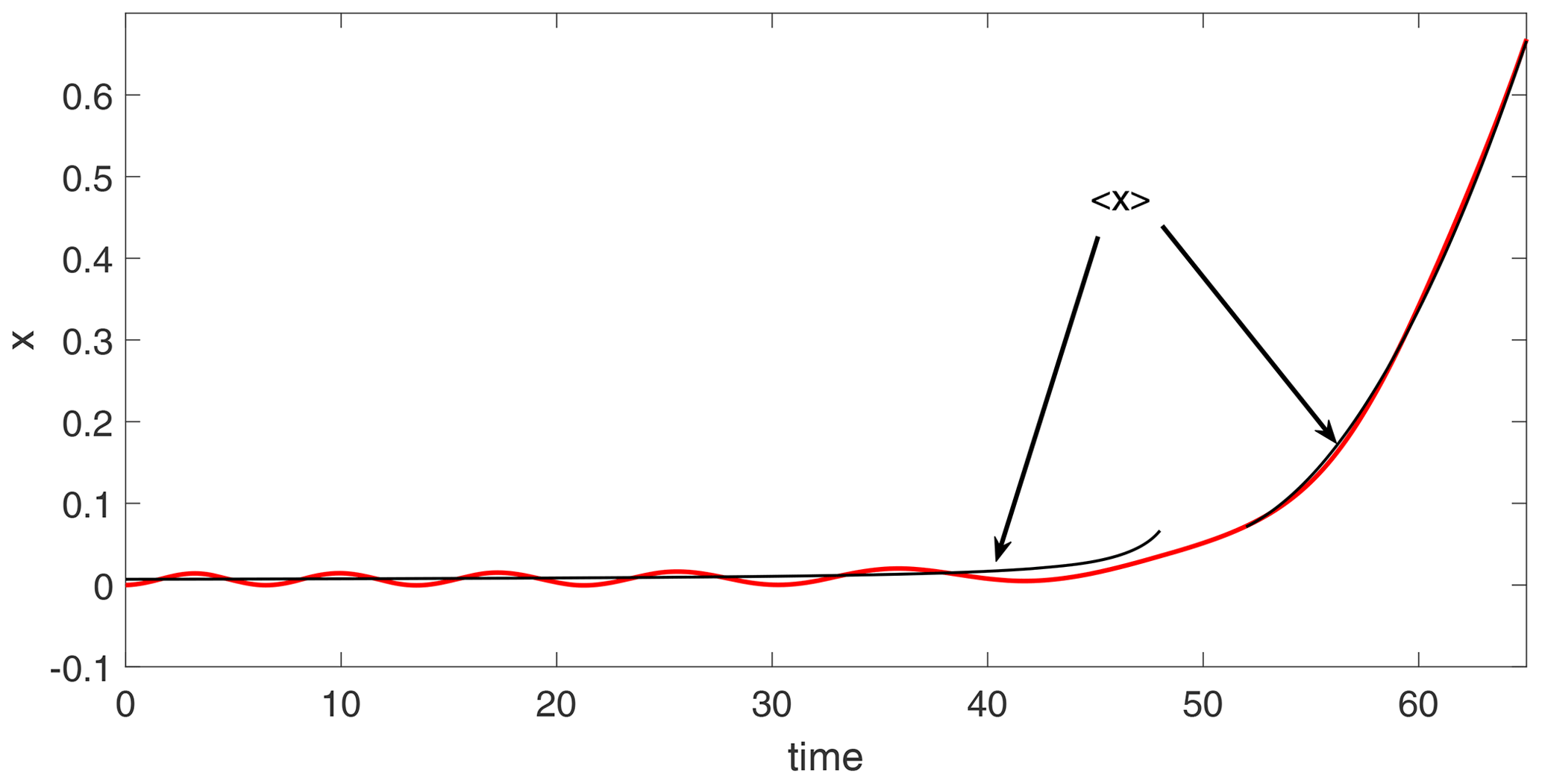
Figure 4 Numerical solutions of x(t) in Eqs. (2)–(5) starting from the same initial conditions as in Fig. 3. The two black curves show the monotonic evolution of x described by Eq. (20) for t<t_cr and by Eq. (21) for t>t_cr, where t_cr=50 as in Fig. 3. The black curves terminate near the Equator where the adiabaticity breaks down since the frequency, ω₀, tends to 0 there according to Eq. (15).

This completes our solution for the latitude, y, and we proceed to the longitudinal dynamics. The dynamics in the zonal direction, x, are governed by Eq. (2), which after substitution of Eq. (13) becomes

$$\begin{array}{}\text{(19)}& {\displaystyle \frac{\mathrm{d}x}{\mathrm{d}t}}=\left[D+y_{\mathrm{m}}\left(\mathrm{1}+{\displaystyle \frac{b}{\mathrm{2}}}{y}_{\mathrm{m}}\right)\right]+(\mathrm{1}+b{y}_{\mathrm{m}})\mathit{\delta }y+{\displaystyle \frac{b}{\mathrm{2}}}\mathit{\delta }{y}^{\mathrm{2}}.\end{array}$$

Here again we consider two cases. For t<t_cr, $D+y_{\mathrm{m}}^{+}(\mathrm{1}+\frac{b}{\mathrm{2}}{y}_{\mathrm{m}}^{+})=\mathrm{0}$, and therefore by averaging locally in time over a single oscillation and using Eqs. (17) and (15), we get

$$\begin{array}{}\text{(20)}& {\displaystyle \frac{\mathrm{d}〈x〉}{\mathrm{d}t}}=-{\displaystyle \frac{b{a}^{\mathrm{2}}}{\mathrm{2}}}+{\displaystyle \frac{F}{{\mathit{\omega }}_{\mathrm{0}}}}.\end{array}$$

This equation shows that the average zonal drift is a nonlinear phenomenon in terms of the amplitude of oscillation. Since, as was shown above, F>0 for t<t_cr, the drift is determined by the balance between $b{a}^{\mathrm{2}}/\mathrm{2}$ and $F/{\mathit{\omega }}_{\mathrm{0}}=b{\mathrm{\Gamma }}^{\mathrm{2}}/{\mathit{\omega }}_{\mathrm{0}}^{\mathrm{4}}$. Thus, the sign (direction) of the zonal drift is independent of the sign of Γ.

For t>t_cr, $y_{\mathrm{m}}^{\mathrm{0}}=-\mathrm{1}/b$, so $D+y_{\mathrm{m}}^{\mathrm{0}}(\mathrm{1}+\frac{b}{\mathrm{2}}{y}_{\mathrm{m}}^{\mathrm{0}})=\mathrm{\Gamma }t-\mathrm{1}/\left(\mathrm{2}b\right)$, and therefore

$$\begin{array}{}\text{(21)}& {\displaystyle \frac{\mathrm{d}〈x〉}{\mathrm{d}t}}=\mathrm{\Gamma }t-{\displaystyle \frac{\mathrm{1}}{\mathrm{2}b}}+{\displaystyle \frac{\mathrm{1}}{\mathrm{4}}}b{a}^{\mathrm{2}}.\end{array}$$

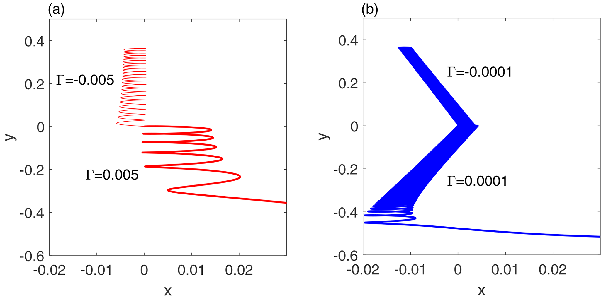
Figure 5 The different water column trajectories for b=2 with initial conditions $x=y=D=\mathrm{0}$ and V=0.002. (a) Large $\left|\mathrm{\Gamma }\right|$ (red curves), (b) small $\left|\mathrm{\Gamma }\right|$ (blue curves). The values of Γ are noted near each of the curves: thin curves denote negative (westward-directed) stresses, and thick curves denote positive (eastward-directed) stresses. The integration time is 2t_cr in all cases, but the curves terminate just prior to reaching the Equator. Note that for Γ=0.00001 the integration time, $\frac{\mathrm{1}}{b\mathrm{\Gamma }}$, is 5000; i.e., the columns in the right panel complete several thousand oscillations in the course of the integration.

Figure 4 displays numerical solutions of x(t) in Eqs. (2)–(5) starting from the same initial conditions as in Fig. 3. The black curves show the monotonic evolution (averaged over oscillations) of x described by the theory developed here. Since the trajectories originate in midlatitudes, a westward-directed wind stress will always stir the trajectories away from the Equator, so Γ in Eq. (21) must be positive; i.e., the long-term zonal drift on the Equator has to be directed eastward.

Figure 5 compares the (x(t),y(t)) trajectories emanating from $x=\mathrm{0}=D=y$ and V=0.002 for two pairs of eastward-directed (thick curves) and westward-directed (thin curves) wind stresses. In the right panel the magnitude of the wind stress is small (0.0001), and in the left panel the magnitude of the wind stress is large (0.005). The two curves in each panel demonstrate that, as concluded above, the zonal drift is independent of the sign (direction) of the wind stress (since according to Eq. 20 it is proportional to F∝Γ²). A comparison between the trajectories in the two panels shows that for tiny wind stress (b) the trajectories drift westward as in the force-free, inertial oscillations, while with the increase in the magnitude of the wind stress (a) the zonal drift is directed eastward. In accordance with the intuits presented in the Introduction on the f-plane solution the oscillation's (inertial) frequency changes with latitude, i.e., increasing or decreasing in northward- or westward-directed trajectories, while the oscillation's amplitude follows the opposite pattern.

4 Discussion and summary

The two simple limits of b=0 (Ekman transport on the f plane) and Γ=0 (inertial trajectories on the β plane) should be discussed as special cases of the present theory. These limits are well known in physical oceanography, but they were never presented as limits of a single dynamical system.

In the b=0 limit (wind forced transport on the f plane) the potential in Eq. (8) becomes $\mathrm{\Phi }\left(y\right)=\frac{\mathrm{1}}{\mathrm{2}}(D+y{)}^{\mathrm{2}}$ (recall that D=Γt). This potential has a single minimum at $y^f=-D$, and the frequency of oscillation near this point is ω^f=1. Near y^f the potential, Φ, is identical to that of the harmonic oscillator: $\frac{\mathrm{1}}{\mathrm{2}}(y-y^f{)}^{\mathrm{2}}$. Thus, the minimum $y^f=-D$ must decrease (or increase, depending on the sign of Γ) indefinitely at a rate that equals Γ; i.e., the potential Φ simply translates in the +y or −y directions without changing its shape.

The Γ=0 limit (inertial trajectories on the β plane) implies, according to Eq. (4), that D is conserved, so the system in Eqs. (2)–(5) has two conserved quantities – D and the energy E. With the increase in the initial energy (say by increasing V(t=0)) the inertial trajectory will oscillate in (V,y) while drifting westward (see Ripa, 1997; Paldor, 2007) as on the sphere (Paldor, 2001). Equation (20) and the trajectories in Fig. 5 show that the long-term westward drift on the β plane when Γ≠0 is slower than in the inertial case, Γ=0, and it is independent of the sign of Γ.

The solutions of the nonlinear system in Eqs. (2)–(5) are determined by the two initial conditions V(t=0) and y(t=0) (recall that $x(t=\mathrm{0})=\mathrm{0}=D(t=\mathrm{0})$ can be assumed without loss of generality since x does not affect the dynamics and D can be translated in time) and the values of the two parameters, b and Γ (that represent the dimensional parameters β and τ^x, respectively), for a total of four parameters! Thus, these solutions display a range of temporal evolution, and this work describes and analyzes the general properties of these solutions and illustrates them in numerical examples. In particular, the zonal drift of the trajectories can be eastward (as in Fig. 1 and the left panel of Fig. 5) or westward (as in the right panel of Fig. 5). The sensitive dependence of the drift on parameter values (including initial conditions) is a defining property of nonlinear systems such as that studied here.

The intent of the analysis in this work is to provide an overview of the complex phenomena that result from the extension of Ekman's theory to the β plane. In particular, this work shows that the zonal drift is independent of the sign of τ^x but depends on a (previously unknown) balance between V(0)² (or the initial displacement from $(y_{\mathrm{m}}^{+}{)}^{\mathrm{2}}$) and (τ^x)². The values of the parameters used in the numerical results presented here were chosen to highlight the phenomena being discussed while still being realistic. Thus, with the velocity scale of f₀R_e=640 m s⁻¹ the value of V(0)=0.002 used in Figs. 3–5 corresponds to a dimensional velocity of about 1 m s⁻¹. Trajectories of much higher oscillation amplitudes will be encountered with higher V(0) values.

The symmetry between $y_{\mathrm{m}}^{+}$ and $y_{\mathrm{m}}^{-}$ in the present theory suggests that for the same wind stress, Γ, the Southern Hemisphere's fixed point will also move towards the Equator, i.e., northward. However, in all other respects the evolution near $y_{\mathrm{m}}^{-}$ is identical to that described above for $y_{\mathrm{m}}^{+}$. The importance of latitudes at which the curl of the wind stress vanishes, which play a fundamental role in Stommel (1948) vorticity-based theory of wind-driven ocean gyres, cannot be captured in extensions of the present Lagrangian theory. However, extensions of the present new Lagrangian theory on the β plane can include variable zonal wind stress, τ^x(y), which can highlight the role played by latitudes at which the wind stress itself vanishes. The application of the concepts developed here to spherical geometry and to wind-driven circulation over the continental shelf (where the sloping bottom yields the topographic β effect) is an interesting goal for future studies.

Appendix A: Adiabatic evolution of meridional oscillations and initial conditions

In this Appendix we discuss adiabatic (slow) evolution of linear longitudinal oscillations described by (see Eq. 14)

$$\begin{array}{}\text{(A1)}& {\displaystyle \frac{d^{\mathrm{2}}\mathit{\delta }y}{\mathrm{d}{t}^{\mathrm{2}}}}=-{\mathit{\omega }}_{\mathrm{0}}^{\mathrm{2}}\left(t\right)\mathit{\delta }y+{\displaystyle \frac{F}{{\mathit{\omega }}_{\mathrm{0}}^{\mathrm{2}}}}\end{array}$$

and seek the solution of this equation of the form

$$\begin{array}{}\text{(A2)}& \mathit{\delta }y=a\left(t\right)\cos \left(\underset{\mathrm{0}}{\overset{t}{\int }}{\mathit{\omega }}_{\mathrm{0}}\left(t\right)\mathrm{d}t+{\mathit{\varphi }}_{\mathrm{0}}\right)+{\displaystyle \frac{F}{{\mathit{\omega }}_{\mathrm{0}}^{\mathrm{2}}}}.\end{array}$$

Here ϕ₀ is added to take into account initial conditions, and we assume that the change in ω₀ during one period $\mathrm{2}\mathit{\pi }/{\mathit{\omega }}_{\mathrm{0}}$ of oscillations is small, i.e.,

$$\begin{array}{}\text{(A3)}& {\displaystyle \frac{\mathrm{d}{\mathit{\omega }}_{\mathrm{0}}}{\mathrm{d}t}}{\displaystyle \frac{\mathrm{2}\mathit{\pi }}{{\mathit{\omega }}_{\mathrm{0}}}}\ll {\mathit{\omega }}_{\mathrm{0}},\end{array}$$

which is guaranteed if Γ is sufficiently small. This is our adiabaticity criterion. A similar condition, $\frac{\mathrm{d}a}{\mathrm{d}t}\frac{\mathrm{2}\mathit{\pi }}{{\mathit{\omega }}_{\mathrm{0}}}\ll a$, is also assumed for the amplitude of oscillations. Next, we substitute Eq. (A2) into Eq. (A1) and neglect $d^{\mathrm{2}}a/\mathrm{d}{t}^{\mathrm{2}}$ to get

$$\begin{array}{}\text{(A4)}& \mathrm{2}{\displaystyle \frac{\mathrm{d}a}{\mathrm{d}t}}{\mathit{\omega }}_{\mathrm{0}}+a{\displaystyle \frac{\mathrm{d}{\mathit{\omega }}_{\mathrm{0}}}{\mathrm{d}t}}=\mathrm{0},\end{array}$$

yielding

$$\begin{array}{}\text{(A5)}& {\mathit{\omega }}_{\mathrm{0}}{a}^{\mathrm{2}}=I=\mathrm{const}.\end{array}$$

The constant I (the action) is given by initial conditions. When the nonlinear terms in Eq. (14) are included in the analysis, the entire derivation of the weakly nonlinear solution as described in pages 86–87 of Landau and Lifshitz (1982) is not affected by the replacement of the linear component acos (ωt+ϕ₀) by $a\left(t\right)\cos \left({\int }_{\mathrm{0}}^t\mathit{\omega }\right(t)\mathrm{d}t+{\mathit{\varphi }}_{\mathrm{0}})$ in the adiabatic problem, which is the basis of the solution in Eq. (17) in Sect. 3.

Finally, the action I, which remains constant all times, can be calculated from the initial conditions, δy(0) and $V\left(\mathrm{0}\right)=\mathrm{d}\left(\mathit{\delta }y\right)/\mathrm{d}t{\mathrm{|}}_{t=\mathrm{0}}$. Using Eq. (A2) we have $\mathit{\delta }y\left(\mathrm{0}\right)=a\left(\mathrm{0}\right)\cos {\mathit{\varphi }}_{\mathrm{0}}+F\left(\mathrm{0}\right)/{\mathit{\omega }}_{\mathrm{0}}^{\mathrm{2}}\left(\mathrm{0}\right)$ and $V\left(\mathrm{0}\right)=-a\left(\mathrm{0}\right){\mathit{\omega }}_{\mathrm{0}}\left(\mathrm{0}\right)\sin {\mathit{\varphi }}_{\mathrm{0}}$. Then

$$\begin{array}{}\text{(A6)}& a(\mathrm{0}{)}^{\mathrm{2}}={\left(\mathit{\delta }y\left(\mathrm{0}\right)-{\displaystyle \frac{F\left(\mathrm{0}\right)}{{\mathit{\omega }}_{\mathrm{0}}^{\mathrm{2}}\left(\mathrm{0}\right)}}\right)}^{\mathrm{2}}+{\left({\displaystyle \frac{V\left(\mathrm{0}\right)}{{\mathit{\omega }}_{\mathrm{0}}\left(\mathrm{0}\right)}}\right)}^{\mathrm{2}}\end{array}$$

and

$$\begin{array}{}\text{(A7)}& I={\mathit{\omega }}_{\mathrm{0}}\left(\mathrm{0}\right){\left(\mathit{\delta }y\left(\mathrm{0}\right)-{\displaystyle \frac{F\left(\mathrm{0}\right)}{{\mathit{\omega }}_{\mathrm{0}}^{\mathrm{2}}\left(\mathrm{0}\right)}}\right)}^{\mathrm{2}}+{\displaystyle \frac{V^{\mathrm{2}}\left(\mathrm{0}\right)}{{\mathit{\omega }}_{\mathrm{0}}\left(\mathrm{0}\right)}}.\end{array}$$

The case depicted in Figs. 3 and 4 has δy(0)=0, so one gets $a^{\mathrm{2}}\left(\mathrm{0}\right)=\frac{F^{\mathrm{2}}\left(\mathrm{0}\right)+V^{\mathrm{2}}\left(\mathrm{0}\right)}{{\mathit{\omega }}_{\mathrm{0}}^{\mathrm{2}}\left(\mathrm{0}\right)}$ and I=ω₀(0)a²(0).