Assessing the capability of three different altimetry satellite missions to observe the Northern Current by using a high-resolution model

Over the last 3 decades, satellite altimetry has observed sea surface height variations, providing a regular monitoring of the surface ocean circulation. Altimetry measurements have an intrinsic signal-to-noise ratio that limits the spatial scales of the currents that can be captured. However, the recent progress made on both altimetry sensors and data processing allows us to observe smaller geophysical signals, offering new perspectives in coastal areas where these structures are important.

In this methodological study, we assess the ability of three altimeter missions with three different technologies to capture the Northern Current (northwestern Mediterranean Sea) and its variability, namely Jason-2 (Ku-band low-resolution-mode altimeter, launched in 2008), SARAL/AltiKa (Ka-band low-resolution-mode altimeter, launched in 2013) and Sentinel-3A (synthetic aperture radar altimeter, launched in 2016). Therefore, we use a high-resolution regional model as a reference.

We focus along the French coast of Provence, where we first show that the model is very close to the observations of high-frequency radars and gliders in terms of surface current estimates.

In the model, the Northern Current is observed 15–20 km from the coast on average, with a mean core velocity of 0.39 m s⁻¹. Its signature in terms of sea level consists of a drop whose mean value at 6.14^∘ E is 6.9 cm, extending over 20 km. These variations show a clear seasonal pattern, but high-frequency signals are also present most of the time. In comparison, in 1 Hz altimetry data, the mean sea level drop associated with the Northern Current is overestimated by 3.0 cm for Jason-2, but this overestimation is significantly less with SARAL/AltiKa and Sentinel-3A (0.3 and 1.4 cm respectively). In terms of corresponding sea level variability, Jason-2 and SARAL altimetry estimates are larger than the model reference (+1.3 and +1 cm respectively), whereas Sentinel-3A shows closer values (−0.4 cm). When we derive geostrophic surface currents from the satellite sea level variations without any data filtering, in comparison to the model, the standard deviations of the velocity values are also very different from one mission to the other (3.7 times too large for Jason-2 but 2.4 and 2.9 times too large for SARAL and Sentinel-3A respectively). When low-pass filtering altimetry sea level data with different cutoff wavelengths, the best agreement between the model and the altimetry distributions of velocity values are obtained with a 60, 30 and 40–50 km cutoff wavelength for Jason-2, SARAL and Sentinel-3A data respectively. This study shows that using a high-resolution model as a reference for altimetry data allows us not only to illustrate how the advances in the performances of altimeters and in the data processing improve the observation of coastal currents but also to quantify the corresponding gain.

1 Introduction

Since the beginning of the 90s, satellite altimetry has enabled many regional circulation studies (e.g. Troupin et al., 2015; Vignudelli et al., 2000, in the NW Mediterranean Sea; Gourdeau et al., 2017, in the Solomon Sea; Liu et al., 2018, in the South China Sea, etc.). Its main advantages are its long-term and regular temporal coverage and its synoptic character. Large-scale structures (>150 km) are well captured with this observational technique which has a crucial role in the knowledge of the circulation at a global scale (Fu and Le Traon, 2006). On the contrary, mesoscale and submesoscale processes such as eddies and meanders or narrow coastal currents are historically poorly resolved by altimetry and generally documented by in situ observations or numerical models (e.g. for the NW Mediterranean Sea – Casella et al., 2011; Guihou et al., 2013; Juza et al., 2013; Ourmières et al., 2011; Schroeder et al., 2011). However, during past years, new altimetry techniques have emerged, specifically the use of the Ka-band frequency with the SARAL/AltiKa mission (2013+), the adoption of the synthetic aperture radar (SAR) mode with CryoSat-2 (2010+), Sentinel-3A,B (2016+, 2018+) and Sentinel-6 (2020+), and a Ka-band radar interferometer (KaRIn) with Surface Water and Ocean Topography (SWOT) (launched in December 2022). In addition, improvements in re-tracking of radar waveforms and a better characterization and removal of geophysical corrections such as atmospheric effects or tidal signals have all served to improve the precision of the data retrieved. All this progress has led to a significant gain in the observability of the fine-scale ocean structures in general and of the coastal features in particular (Birol et al., 2021; Morrow et al., 2017; Verron et al., 2018).

Despite the progress made, intercomparisons with in situ observations of near-coastal currents have shown that the corresponding altimetry-derived surface velocities are underestimated (Birol et al., 2010; Jebri et al., 2016). In Carret et al. (2019), using long time series of both ADCP (acoustic Doppler current profiler) and glider data as a reference for the Northern Current (NC hereinafter) velocities, we have shown that satellite altimetry data underestimate the amplitude of NC seasonal variations by ∼40 %–45 %. This can be explained by the ageostrophic current component, not captured by altimetry, but also by the effective data resolution, which is limited by the altimeter noise and coastal-data-processing issues, resulting in near-shore data gaps. This limitation decreases with new radar techniques and data-processing approaches (Birol et al., 2021; Morrow et al., 2017). Nevertheless, there is a need to specify more precisely the corresponding improvements in coastal observability. It is particularly important to optimize the use of altimetry in near-shore areas and to finally define its place among other coastal observation systems.

As satellite altimetry measures sea surface height (SSH or sea level hereinafter), the observability condition is that the processes of interest have a sea level signature and spatio-temporal scales larger than the altimetry resolution. Over the open ocean, the altimetric observability problem is generally studied through a spectral approach (Dufau et al., 2016; Morrow et al., 2017; Vergara et al., 2019). This gives a mean statistical solution over the considered region but can not be used in the coastal ocean where too-short satellite track sections often impede the computation of a spatial spectral analysis. Several studies (Bouffard et al., 2008; Carret et al., 2019; Pascual et al., 2015; Troupin et al., 2015) have used in situ observations to analyse the resolution capability of coastal altimetry data, but they came up against the scarcity of independent measurements and their non-colocation in space and/or time.

In this paper, we propose a different strategy based on a high-resolution numerical model. Our purpose is to assess the ability of satellite altimetry, using three different technologies, to observe a particular coastal dynamical structure. Using a high-resolution model may overcome the issue of colocation between in situ and altimetry data but given the essential condition that the physical process studied must be correctly represented by the model. Our methodology relies first on a careful model validation step in the study region. Then, the model is considered as a reference. Our approach will consist of using the model to quantify the SSH signature of an identified physical process along a particular satellite track. In a second step, the model solution will be compared with the SSH signature captured in the altimetry dataset along the considered tracks and with the resulting geostrophic currents.

As in Carret et al. (2019), the case study chosen is the NC in the northwestern Mediterranean Sea (NWMed hereinafter). This region is indeed considered as a laboratory area for coastal altimetry studies (Birol et al., 2010; Birol and Delebecque, 2014; Bouffard et al., 2008) because of its small Rossby radius (around 10 km; Grilli and Pinardi, 1998), leading to a wide variety of mesoscale and submesoscale structures. We can also benefit from the variety of in situ data collected from the MOOSE (Mediterranean Ocean Observing System for the Environment, https://www.moose-network.fr/ (last access: 16 March 2023), Tintoré et al., 2019) integrated observing system and from the long experience and really good performances previously obtained with the high-resolution SYMPHONIE numerical model in the study area (Damien et al., 2017; Estournel et al., 2016; Herrmann et al., 2008).

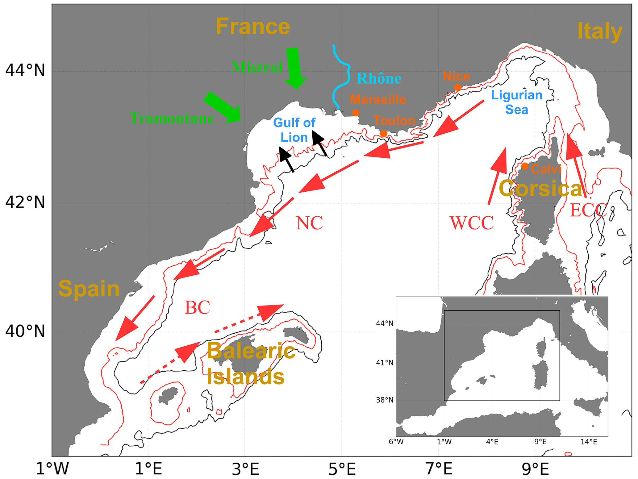
Figure 1 Map of the schematic circulation in the northwestern Mediterranean study area, with inset map showing the location of the main map (outlined by a black box). Red arrows indicate the main currents; black arrows indicate the intrusion in the Gulf of Lion; 200 m (red line) and 1000 m (black line) isobaths are also shown. The geographic features mentioned in the text are indicated. NC – Northern Current; BC – Balearic Current; WCC – Western Corsica Current; ECC – Eastern Corsica Current.

The NC is a narrow slope current (Fig. 1) formed by the junction of the Eastern Corsica Current (ECC) and the Western Corsica Current (WCC) in the Ligurian Sea (Taupier-Letage and Millot, 1986). It flows cyclonically along the Italian, French and Spanish coasts (Millot, 1987). It has a strong seasonal component with a maximal and minimal transport (maximum of 1.6 Sv; Alberola et al., 1995) and increased mesoscale variability in winter and summer (e.g. Crépon et al. 1982; Flexas et al. 2002; Sammari et al., 1995). Its position relative to the coast also varies through the year, from less than 20 km from the coast from spring to early November to about 30 km from the coast in November and December (Niewiadomska, 2008; Sammari et al., 1995). Its depth and width also show marked seasonal variations at more than 200 m in winter and 150–200 m during the rest of the year for the depth and 30 km in general with a narrowing in winter (Alberola et al., 1995) for the width.

In the past, the NC variability has been intensively studied with in situ observations and models – mesoscale fluctuations at 3–6 and 10–20 d in Sammari et al. (1995), month-long eddies in Casella et al. (2011) and Hu et al. (2011), and day-long eddies in Schaeffer et al. (2011). Birol et al. (2010) have highlighted the contribution of along-track satellite altimetry to studying the NC seasonal variability. Since then, other altimetry studies have used such data to investigate the NC circulation, as well as the recirculation and associated meanders (case studies in Borrionne et al., 2019; Morrow et al., 2017; Pascual et al., 2015). However, none of them have clearly quantified the observation limit (in both space and time), probably due to the lack of independent sea level and/or current datasets to do so.

Here, we will investigate in detail the NC observability issue for three altimetry missions associated with different techniques, namely Jason-2, with the classical Ku-band low-resolution mode (LRM) nadir altimeter; SARAL, which uses the Ka-band frequency in LRM; and Sentinel-3A (Sentinel-3 hereinafter), with its synthetic aperture radar mode. Section 2 describes the study tools and the model validation step. Section 3 presents the methodology used to quantify the NC sea level signature in the Ligurian Sea and in the area south of Toulon and the results obtained. Section 4 focuses on the NC observation with the three altimetry missions and analyses the differences obtained between altimetry and the model. Section 5 summarizes and concludes the paper.

2 Data

In this study, in situ (glider), high-frequency (HF) radar and satellite altimetry data are first used to validate a regional numerical simulation. Our study period, strongly constrained by both the in situ data and the model simulation availability, goes from 2011 to 2019. The different observing platforms and the model are presented in Sect. 2.1 and 2.2 respectively. Results of the model validation are provided in Sect. 2.3.

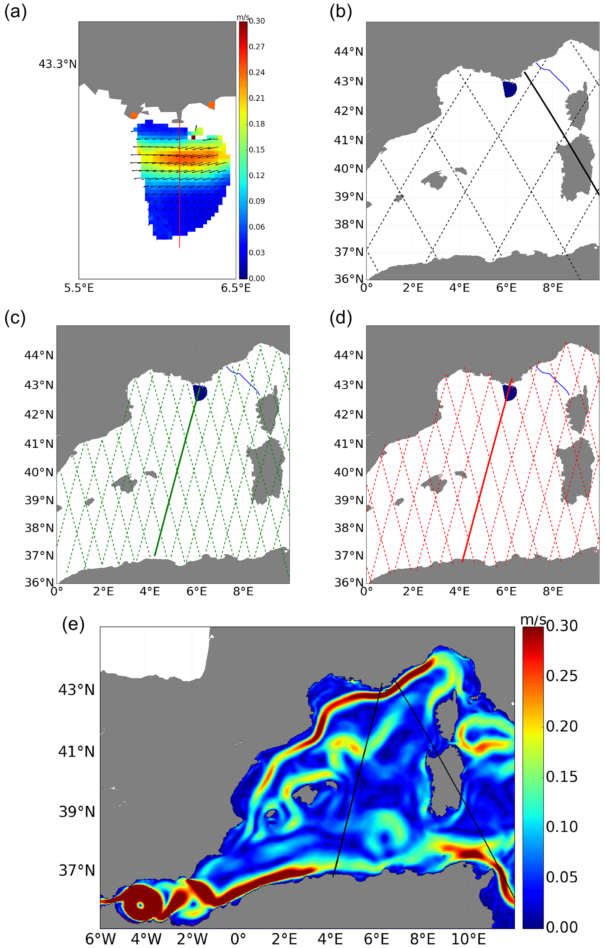
Figure 2 Maps illustrating the location of the observations used in this study, as well as the spatial model coverage. (a) Mean surface current velocity map from the HF radars near Toulon over 1 May 2012 to 30 September 2014; the red line shows the transect used in the study, and the orange dots show the location of the antennas. Altimetry tracks in the western Mediterranean Sea for (b) Jason-2, (c) SARAL and (d) Sentinel-3. For each mission, the tracks used in the study (track 222 for Jason-2, track 302 for SARAL and track 472 for Sentinel-3) are indicated in bold. The HF radars coverage area and the Nice–Calvi glider transect are represented in blue. (e) Mean surface current intensity from the SYMPHONIE model for the period 18 May 2011–31 March 2017. The satellite tracks are represented in black.

2.1 In situ instruments and satellite altimetry

2.1.1 HF radars

We took advantage of the 2 years of data, from May 2012 to September 2014, provided by the HF Wellen RAdar (WERA) instruments installed near Toulon as part of the MOOSE network (https://doi.org/10.17882/56500; Zakardjian and Quentin, 2018). The measurements correspond to the dataset available at the time of the study. The stations (in orange in Fig. 2a) are located in Cap Sicié and Cap Bénat-Porquerolles in respectively monostatic and bistatic eight-antenna configurations (now upgraded to 12 antennas by site). Their positions enable the monitoring of the NC upstream of the Gulf of Lion (Fig. 2a) and the mesoscale dynamics that occur in this region of cross-shelf exchanges and strong atmospheric forcing (Mistral, Tramontane winds). They operate at 16 MHz with a 50 kHz bandwidth, resulting in a spatial resolution of 3 km, and allow an angular resolution of 2^∘. The HF radars provide the surface current every hour over a region of 60×40 km. Data are then filtered from tides and inertial oscillations, edited, averaged daily, and finally binned on a regular 2×2 km grid (see Zakardjian and Quentin, 2018 for more details). Note that this data processing removed part of the high-frequency currents (not captured by altimetry that observe only geostrophic currents).

2.1.2 Gliders

In the NWMed, a number of gliders have been deployed since 2005 along different transects, measuring temperature and salinity vertical profiles. We focus on a regular line, from Nice to Calvi, where 36 deployments occurred from 2009 to 2016 as part of the MOOSE network. From 2011 to 2017, there are 204 sections. Data were treated according to Carret et al. (2019), who discarded profiles that were too short or deviated too much from an average Nice–Calvi trajectory. The treatment results in temperature and salinity data down to 500 m (depth reached by all gliders), gridded with a 4 km horizontal bin size along the mean trajectory considered as a reference track. The temperature and salinity data are then filtered using a 15 km cutoff wavelength. The geostrophic velocity component perpendicular to the reference track is then derived using the thermal wind equation referenced to 500 m (see Carret et al., 2019, for further details).

2.1.3 Satellite altimetry

Jason-2 was launched in June 2008 and was in the same orbit up to October 2016. It is based on the conventional LRM altimeter operating in the Ku-band and has a 10 d repetition cycle. SARAL, launched in February 2013, provides a shorter data time series (∼3 years) because it moved to a drifting orbit in July 2016. It has a 35 d repeat observation cycle. Its Ka-band LRM altimeter (called AltiKa) has a smaller footprint than the Ku-band instruments, specifically a ∼4 km radius against 5–7 km. The corresponding lower data noise allows the capture of smaller spatial scales in comparison to Jason-2 (Verron et al., 2018). The Ka-band is also less affected when crossing the ionosphere and provides a better estimation of the surface roughness. Sentinel-3 was launched in February 2016. With its synthetic aperture radar (SAR) altimeter, its footprint is even more reduced in the along-track direction compared to LRM altimeters (∼0.3 km). It has a 27 d repeat observation cycle.

Table 1 Characteristics of the altimetry datasets used in this study as a function of the satellite mission.

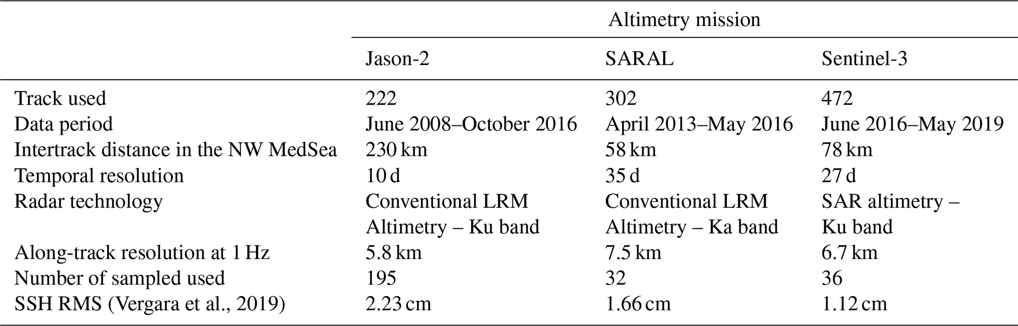
Figure 2b–d indicates the satellite tracks of each mission in the NWMed, defining the spatial coverage of the corresponding nadir altimetry observations. Note that the spatial resolution of nadir 1 Hz altimetry data is in the range 5–8 km along the track (Table 1), but the inter-track distance varies from 230 km for Jason-2 to 76 km for Sentinel-3 and 58 km for SARAL. For each mission, the tracks used in this study are indicated in bold in Fig. 2b–d. They correspond to the tracks closest to HF radar data (see below for explanation); the Sentinel-3 track 472 and the SARAL track 302 pass over the HF radar region with a different angle, whereas the Jason-2 track 222 is located a bit further to the east at about 60 km. As along-track altimetry data allow one to derive only the across-track currents, through the geostrophic assumption, the angle of the track with respect to the current vein has a major impact on the current capture – specifically, the less perpendicular the track, the less realistic the amplitude. Concerning SAR altimeters, the observation of a current perpendicular to the track will benefit from the corresponding increase in resolution. Table 1 summarizes the characteristics of each altimetry dataset.

For all missions, we use the X-TRACK along-track sea level anomaly (version 1.02, 2017, https://doi.org/10.6096/CTOH_X-TRACK_2017_02) regional product processed with a coastal-oriented strategy described in Birol et al. (2017). It provides 1 Hz sea level anomaly (SLA) time series homogeneously processed and regularly spaced (Table 1, along-track resolution) along the different satellite tracks. The processing is the same for all missions, except that the dual-frequency of Jason-2 and Sentinel-3 altimeters allows the ionosphere correction to be computed, whereas a model is required for SARAL. With this correction being associated with long wavelengths, it should not impact the results obtained in this study.

To obtain the absolute dynamic topography (ADT), the X-TRACK SLA data are added to a regional mean dynamic topography (SMDT-MED-2014, developed by Rio et al., 2014). Then the absolute across-track geostrophic velocity (u) is derived from the geostrophic equation (Eq. 1) as follows:

$$\begin{array}{}\text{(1)}& u={\displaystyle \frac{-g}{f}}{\displaystyle \frac{\mathrm{\Delta }\left(\text{SLA}+\text{MDT}\right)}{\mathrm{\Delta }x}},\end{array}$$

where g is the gravitational constant, f is the Coriolis parameter, and Δx is the distance between the 1 Hz altimetry points. Before adding the MDT and computing current estimates, the SLA may be filtered in the along-track direction in order to remove the remaining altimetry noise. To investigate the data noise issue, both unfiltered and filtered 1Hz SLA data have been considered for the computation of geostrophic velocities in Sect. 4.1 and 4.2 respectively. The filtering is done with a low-pass Loess filter using different cut-off wavelengths (see Sect. 4.2) .

2.2 Model

We rely here on the SYMPHONIE primitive-equation model which has been widely used in the study area at the nearshore (Michaud et al., 2012), coastal (Estournel et al., 2003; Mikolajczak et al., 2020; Petrenko et al., 2008) and regional (Estournel et al., 2016) scales. Validation studies of SYMPHONIE currents over the Gulf of Lion have been carried out by comparison with various instruments on different hydrological structures and meteorological situations, specifically VHF radars on the Rhone plume (Estournel et al., 2001), hull-mounted ADCP (Estournel et al., 2003) in prevailing northerly winds, fixed ADCP (Mikolajczak et al., 2020) and glider drift (Gentil et al., 2022) during easterly storms.

SYMPHONIE is described in Marsaleix et al. (2008, 2006) and in Damien et al. (2017), with turbulence closure and convection parameterization detailed in Estournel et al. (2016). The configuration used in this study covers the whole Mediterranean basin and the Marmara Sea and extends westward up to 8^∘ W in the Gulf of Cadiz, as described in Estournel et al. (2021). The horizontal resolution is minimal (2 km) in the northwestern Mediterranean (except for a local narrowing at the Strait of Gibraltar). A VQS (vanishing quasi-sigma) vertical coordinate (Estournel et al., 2021) with 50 levels is used. The model is initialized and forced at its open boundaries with an analysis produced by the operational oceanography centre Mercator Ocean International (MOI; Lellouche et al., 2013). As stratification is crucial for mesoscale characteristics, it has been debiased from observations collected over the whole basin, as in Estournel et al. (2016), while preserving the first 100 m, which benefits optimally from the data assimilation performed at MOI. At the air–sea interface, the hourly forecasts of ECMWF (European Centre for Medium-Range Weather Forecasts) based on the high-resolution 10 d forecast (HRES product) at the horizontal resolution of 0.125^∘ are used to calculate heat and momentum fluxes through bulk formulae.

The model simulation covers the period from 18 May 2011 to 31 March 2017 and provides 4 d averaged fields.

2.3 SYMPHONIE model assessment

The model performance in representing the NC velocity field in the study area is assessed quantitatively in terms of statistics (time average and standard deviation) and qualitatively in terms of the complete range of variability (Hovmöller diagrams).

For the comparison with the HF radars, we consider the zonal-current component from May 2012 to September 2014 along a section located at 6.14^∘ E, just south of Toulon (Fig. 2a). The model equivalent is extracted along this section with the same spatial and temporal resolution as the HF radars. Daily outputs for the model during the HF radar period are used. Note that, due to the coast configuration, in this area, the NC which follows the 1000–2000 m isobaths is mainly westward, i.e. with a dominant zonal component most of the time (with the exception of short-living (3–6 d) meanders or wind-induced instabilities). Figure 3a shows the time average and standard deviation of the zonal velocity as a function of latitude along this section. At this longitude, the NC flows westward and corresponds then to the negative values observed north of 42.7^∘ N. In terms of statistics, there is an excellent agreement between the HF radars and the simulation. On average, the NC position and current amplitude are almost identical in both fields. The mean NC core velocity (called V_max hereinafter) is $-\mathrm{0.44}\pm \mathrm{0.16}$ m s⁻¹ for the simulation and $-\mathrm{0.43}\pm \mathrm{0.19}$ m s⁻¹ for the HF radars. This velocity value, identified as the NC core, is located at 42.85^∘ N for both the simulation and observations. We define the width of the NC as the length of the section around its core where the absolute velocity is larger than $\left|V_{\text{max}}\right|/\mathrm{2}$. On average, it is 18±5.9 km for the simulation and 18±6.1 km for the observations. All these figures are summarized in Table 2. The main difference along the section is that, between the NC and the coast (to the north), the velocity variability is slightly greater for the HF radars than for the simulation.

Table 2 Characteristics of the Northern Current along HF radars and gliders sections.

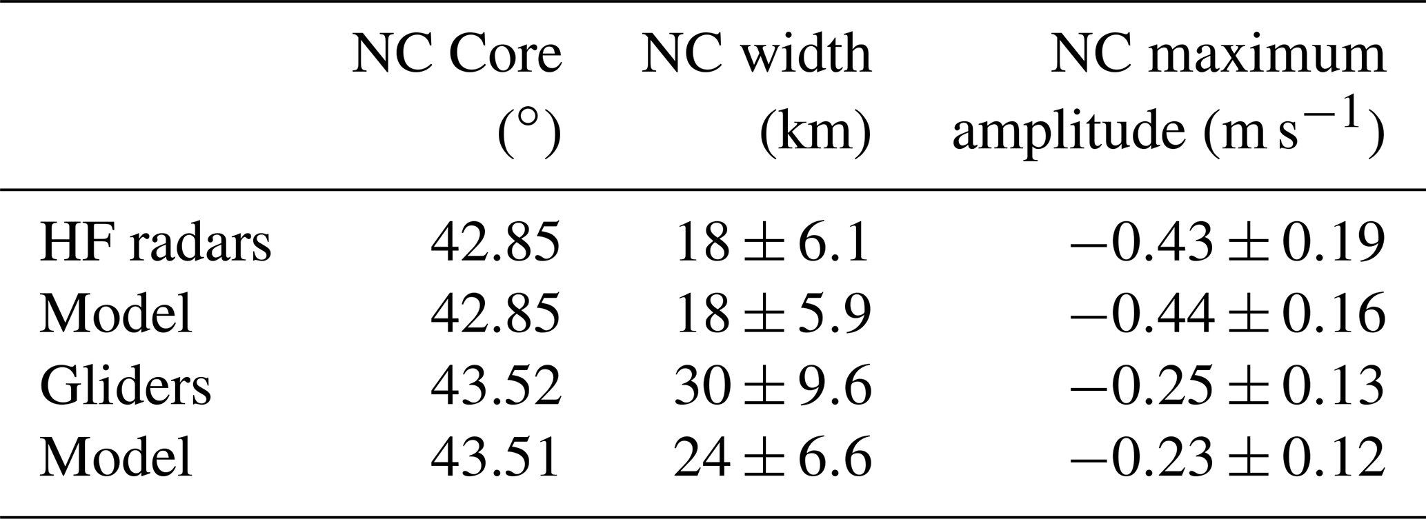
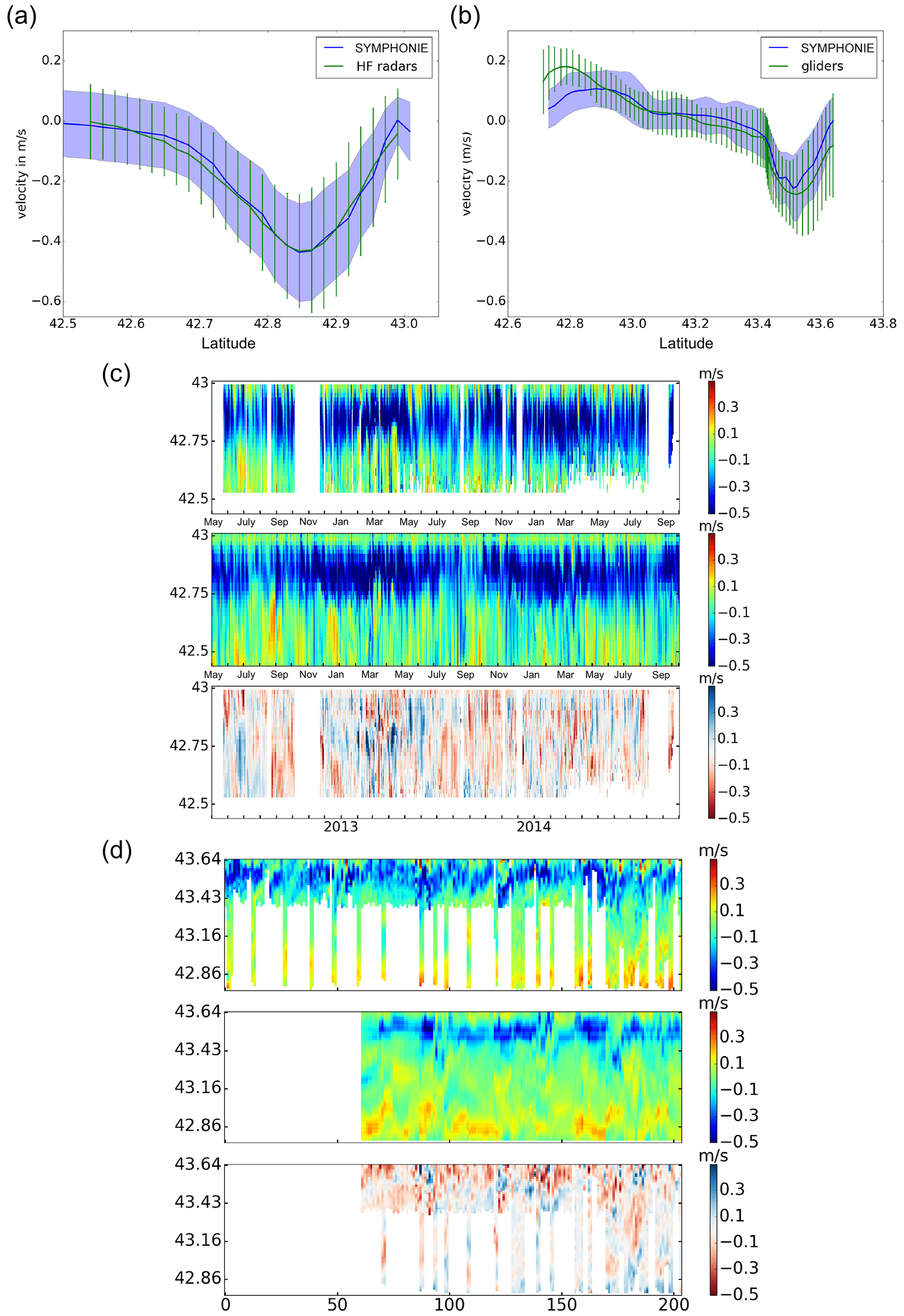
Figure 3 (a) Mean zonal total surface current velocities along a meridional section located at 6.14^∘ E for the simulation in blue and for the HF radars in green over the HF radar period of 1 May 2012–30 September 2014; (b) Mean across-track geostrophic current along the Nice–Calvi line for the simulation in blue and for the gliders in green over 1 January 2011–31 December 2017.The blue envelope and the green bars represent the standard deviation at each point for the model and instruments respectively. Hovmöller diagrams of (c) the zonal-total-current component along a meridional section located at 6.14^∘ E given by the HF radars (top panel of Figure c) and the simulation (middle panel of c) and of (d) the geostrophic current for the gliders (top panel of d) and the simulation at the glider temporal resolution (middle panel of d). The lower panels of (c) and (d) show the differences between the observations and the simulation.

In order to investigate the representation of the NC variability in the simulation in more detail, Fig. 3c represents the Hovmöller diagrams of the zonal velocity along 6.14^∘ E for both the HF radars and the simulation and the differences between both fields. We observe an overall good agreement between the observations and the simulation, with both estimates showing the same seasonal variability, i.e. larger velocities in winter and spring and a summer slow down, and a similar high-frequency variability that may instantiate the wind-induced (Ekman current) and mesoscale (meanders and eddies) variability of the circulation. The differences between the currents' estimates are generally low, and higher values (order of a few tens of centimetres per second) can be largely explained given the fact that short-living structures may not strictly coincide in time and space in the model and observations.

The same diagnostics have been computed for the simulation and the glider data along the Nice–Calvi section, located further east (Fig. 3b, d), but in this case with the geostrophic current component being normal to the section (Table 2). Here, to get as close as possible to the data, we used the vertical temperature and salinity model profiles extracted along the Nice–Calvi section and then computed the geostrophic velocities with the same method as for the gliders. We also observe a good agreement between the simulation and the gliders but with higher differences than what was obtained with the HF radars, especially in terms of current variability. We obtain V_max values of $-\mathrm{0.23}\pm \mathrm{0.12}$ m s⁻¹ for the model and $-\mathrm{0.25}\pm \mathrm{0.13}$ m s⁻¹ for the gliders. Near the coast, the differences between the observed and simulated mean currents can reach 0.1 m s⁻¹. The NC core is located at 43.51^∘ N for the simulation and at 43.52^∘ N for the observations. The NC is thus well located in relation to the coast in the simulation but narrower (24±6.6 km) compared to the observations (30±9.6 km). Concerning the Hovmöller diagrams, the instantaneous differences in velocity between the observations and the simulation can reach 0.5 m s⁻¹. They are associated with a misplaced current in time in the model rather than with incorrect current maxima. The irregular temporal sampling of the gliders also contributes to these larger qualitative model–data differences compared to the HF radar results. Indeed, a deeper analysis shows that the same features may occur in the simulation and in the observations but shifted by 1 or 2 d (not shown). In such cases, they are captured by the daily HF radar equivalent but may correspond to gaps in the irregular glider equivalent.

All these results show that the simulation has excellent skills in terms of circulation, especially at the local circulation in the vicinity of the HF radars and glider-covered areas.

3 Signature of the NC on sea level

The good results obtained above in the Ligurian Sea and south of Toulon in terms of model–data comparison allow us to use the simulation as a reference for altimetry data analysis. It is first used to quantify the NC sea level signature before analysing how it is captured by altimetry data (Sect. 4). We first describe how we quantify this signature using the HF radar zonal section described in Sect. 2.

In the simulation, we first extracted the sea level profile for each date along the section located at 6.14^∘ E (see Fig. 2a). The corresponding cross-transect surface geostrophic-current component is then calculated using Eq. (1), as for classical altimetry estimates.

For each SSH profile, we use three diagnostics to characterize the NC sea level signature. First, the location of the NC core, corresponding to the maximum velocity in absolute value, is spotted on the cross-shore current profile (expressed as a distance to the coast). Then, the drop in SSH (called diff) is computed over the region delimited by velocity values higher than half of the NC core velocity (Eq. 2; Niewiadomska et al., 2008).

$$\begin{array}{}\text{(2)}& \text{diff=max}\left({\text{SSH}}_{\left|u\right|\ge \frac{\left|u\right|\text{max}}{\mathrm{2}}}\right)-\text{min}\left({\text{SSH}}_{\left|u\right|\ge \frac{\left|u\right|\text{max}}{\mathrm{2}}}\right)\end{array}$$

Finally the width (dx) of this region, considered to be the NC width, is derived from the distance between the two half NC core velocities (Niewiadomska, 2008). This criterion offers the advantage of not being impacted by seasonal differences in the NC amplitude.

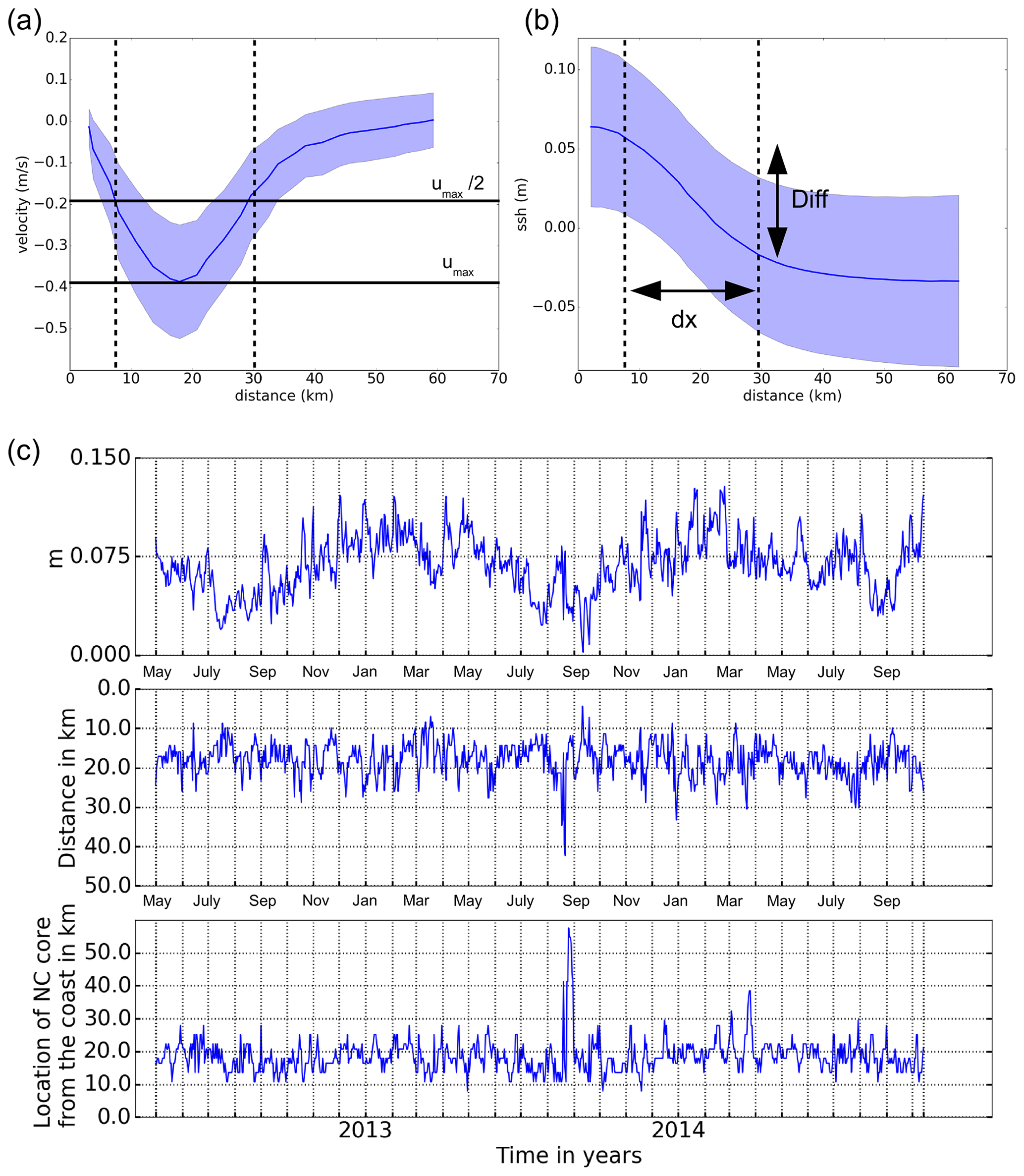
Figure 4 Time-averaged (a) surface current velocities and (b) SSH along a meridional section located at 6.14^∘ E for the SYMPHONIE model over the HF radar period of: 1 May 2012–30 September 2014. (c) Time series of the SSH drop (in m, upper panel), width (in km, middle panel) of the NC and location of the NC core as a function of the distance to the coast (in km, lower panel). The blue envelopes in (a) and (b) represent the standard deviation at each point. The horizontal full lines correspond to the maximum and half the maximum velocity values. The dashed vertical lines delimit the NC width.

Figure 4 illustrates the methodology described above for the model SSH and corresponding zonal current profiles along the 6.14^∘ E transect and averaged over the HF radar period. The profiles are represented as a function of the distance to the coast. In Fig. 4a, the dashed vertical lines delimit the NC width. They are transposed on Fig. 4b in order to derive the corresponding SSH drop (diff value).

We observe that, on average, the SSH decreases from 8 to 28 km to the coast, i.e. the distance dx. This corresponds to the NC associated with negative zonal velocity values. Still, on average, the NC core velocity is −0.39 m s⁻¹ and is about 18 km from the coast. It corresponds to a drop in sea level of 6.9 cm over 20 km. These values are considered to be the mean sea level signature of the NC in the area considered.

The time series of the three diagnostics defined above along the 6.14^∘ E transect are represented in Fig. 4c. The SSH drop associated with the NC varies between 2 and 15 cm, with a clear seasonal tendency. Greater values are generally observed in winter, and smaller values are generally observed in summer. The NC core position varies between 10 and 30 km from the coast (30 km in Alberola et al., 1995) with a slight seasonal variation. It is a little closer to the coast in autumn than in winter, in agreement with Niewiadomska et al. (2008) and Sammari et al. (1995), even if these previous studies were not in the Toulon area. The NC width spreads over 10 to 25 km, depending on the season (it is the widest in January and July and the narrowest in March and April). Previous studies (Alberola et al., 1995) show an NC that is narrower and faster in winter; it may depend on the NC orientation in relation to the section – specifically, an NC not purely perpendicular may artificially increase the current width. In the different diagnostics, the high-frequency variability is also important, with some strong peaks. This may be due to intense wind events which induce meanders or eddies in the HF radars area (Guihou et al., 2013). Note that, in August 2013, the NC core shifted to be 50 km from the coast, associated with a large width and strong SSH drops (Fig. 4c). It is also visible in Fig. 3 for both the simulation and the HF radars. We investigated what happened for the corresponding dates, from 25 to 28 August 2013, in both the simulated and observed surface currents (not shown). We observed that the NC then totally deviated to the south and was cut into two parts, with a recirculation loop that came from the southwest and blocked the NC flow. The good agreement between the model and the HF radars during this extraordinary event is proof of the model's reliability in reproducing the high-frequency variability of the NC.

If we consider the global root-mean-square (rms) error level for the altimetry missions, which is 2.23, 1.66 and 1.12 cm for Jason-2, SARAL and Sentinel-3A respectively (Vergara et al., 2019), the NC signature in terms of SSH corresponds to greater values and thus might be observable. However, its width is generally below the scales resolved. Indeed, Jason satellites can capture offshore dynamical signals down to ∼70 km wavelength, and SARAL/AltiKa and Sentinel-3 satellites can capture offshore dynamical signals down to 35–50 km (Raynal et al., 2017). We also know that the observation of near-shore SSH estimates is a technical challenge for altimetry (Vignudelli et al., 2011). In the next section, using the model as the reference, we analyse which parts of the NC SSH and current signals are really sampled by altimetry data.

4 Observability of the NC in altimetry data: from Jason-2 to Sentinel-3

In this section, a quantitative assessment of the NC sea level signature (in terms of SSH drop, NC width and distance to the coast) is performed for the three altimeter missions and the reference model. We consider both unfiltered (Sect. 4.1) and filtered (Sect. 4.2) 1 Hz SLA data for the computation of geostrophic velocities to analyse the importance of applying spatial filters to altimeter data in order to obtain a better agreement with the model.

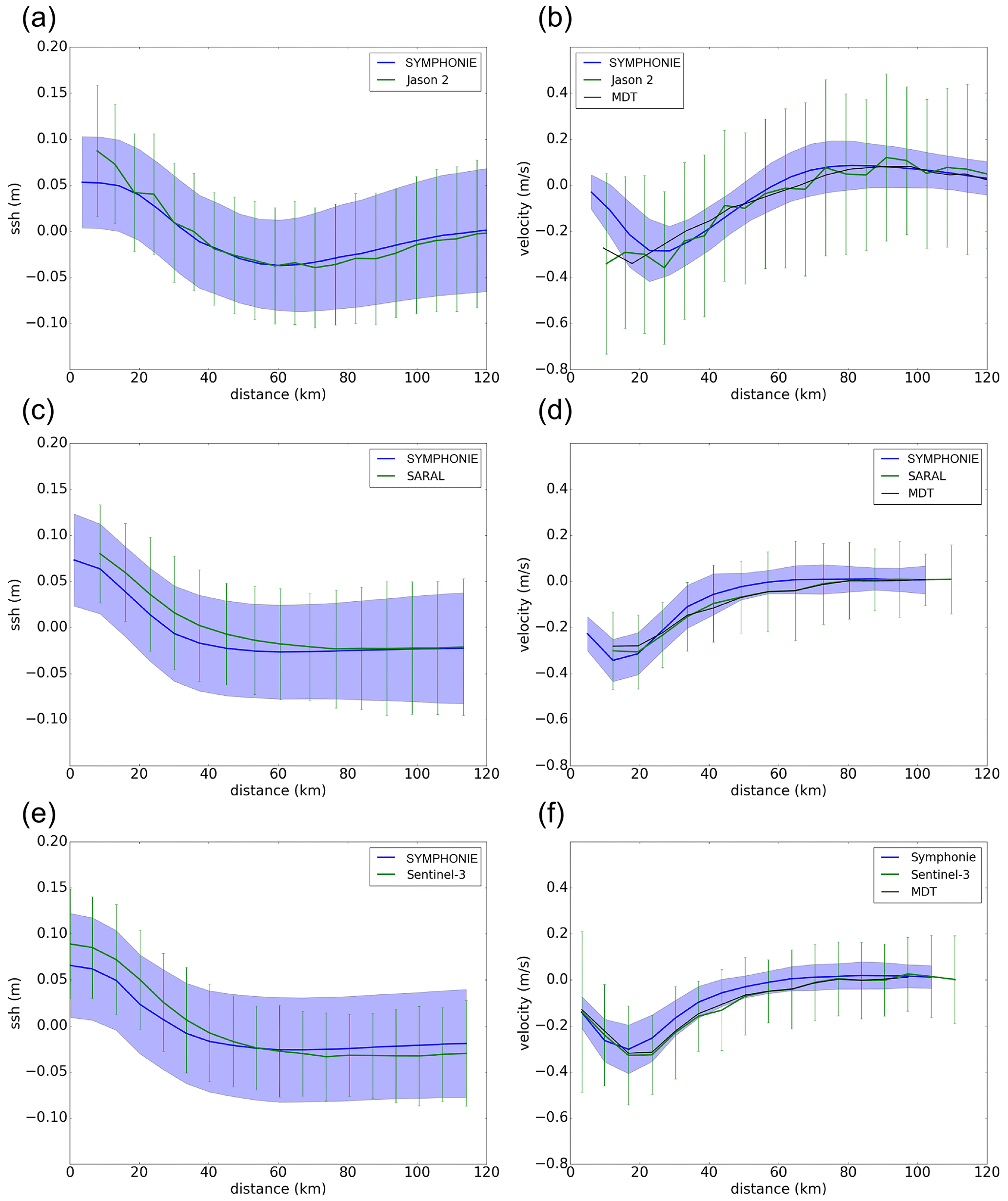
Figure 5 Mean (a), (c), (e) SSH and (b), (d), (f) across-track geostrophic current velocities along (a), (b) Jason-2 track222 over 27 May 2011–1 October 2016, (c), (d) SARAL track 302 over 24 March 2013–13 March 2016 and (e), (f) Sentinel-3 track 472 for the model over 21 June 2014–15 March 2017 in blue and altimetry raw data over 18 June 2016–14 March 2019 in green. The blue envelope and green bars represent the standard deviation at each point for the model and the satellite data respectively. The distance is referenced to the coast. The currents derived from the MDT are added in black in b), (d) and (f).

4.1 SSH and current statistics

We compute the temporal mean and standard deviation of the individual SSHs and corresponding cross-track velocity profiles (using Eq. 1) observed along Jason-2 track 222, SARAL track 302 and Sentinel-3 track 472 (Fig. 5). The corresponding model estimates at the dates closest to altimetry are also calculated and shown in the same figures. The model fields are interpolated at the 1 Hz altimetry points along each track (i.e. every 6–7 km depending on the altimetry mission). Note that, here, no spatial filtering is applied on altimetry data, neither on the SSH nor before computing the geostrophic velocities, because we want to analyse the resolution capability of raw sea level data. The geostrophic current derived from the MDT is also shown in Fig. 5b, d and f to estimate its contribution to the total geostrophic current. For the Jason-2 and SARAL missions, periods were selected based on the joint availability of both observations and model outcomes (see in Table 3). For Sentinel-3, the matching period was very short; thus, the full data availability periods for the observations and model were considered. To estimate the impact of this choice on the results, we performed a sensitivity analysis by computing the mean current and the mean SSH of the model (same diagnostics as those in Fig. 5) over different 3-year time periods, over 10 June 2011–31 March 2014, 22 June 2012–17 March 2015 and 8 June 2013–29 March 2016. The results are very similar (not shown), which indicates that, in this area, the interannual variability does not have a strong imprint on our results.

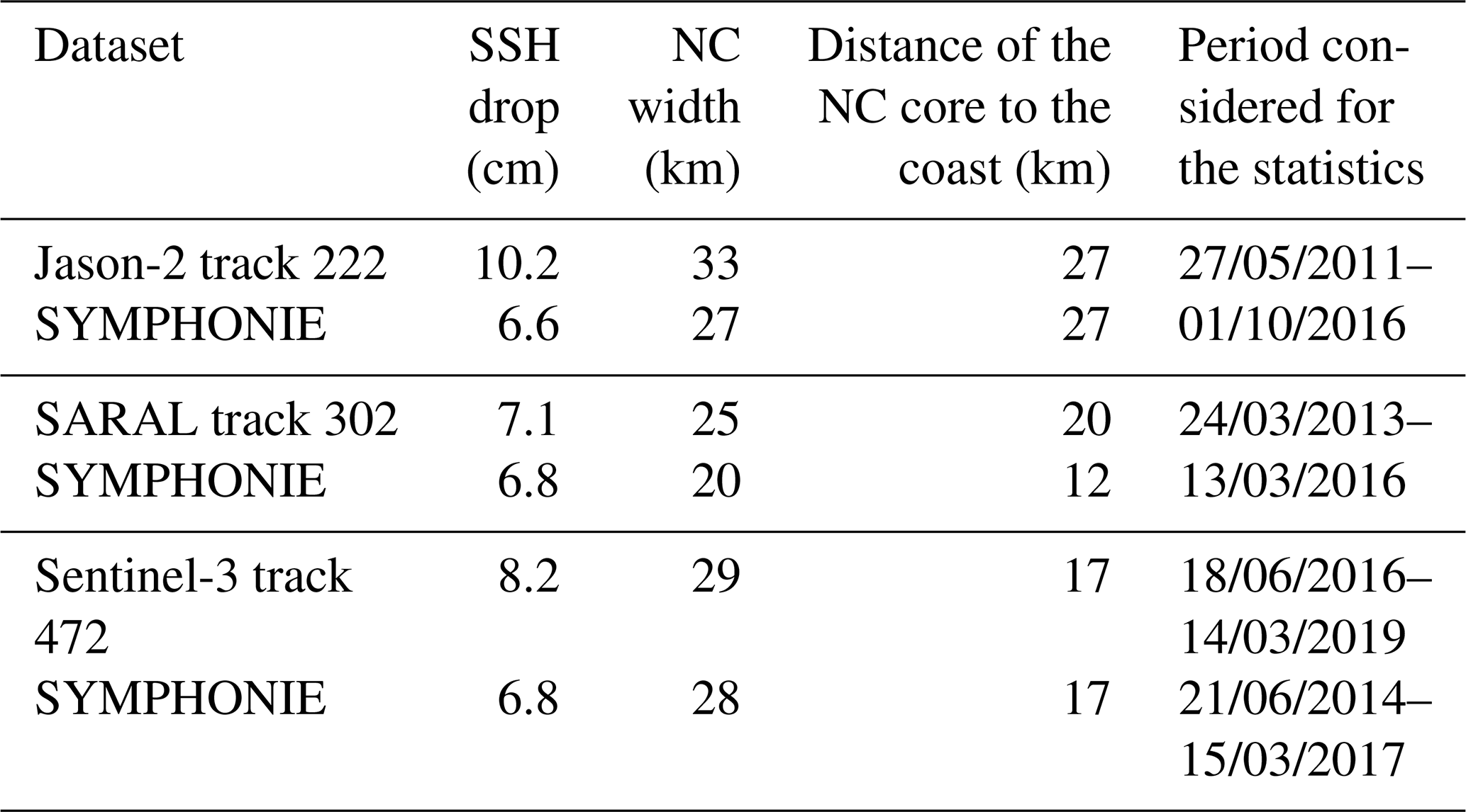
Table 3 Northern Current SSH signature derived from the time-averaged SSH profiles computed along the Jason-2 track 222, the SARAL track 302, the Sentinel-3 track 472 and the equivalent SYMPHONIE sampled as 1 Hz altimetry (SSH drop, NC width and distance to the coast).

The three diagnostics defined in Sect. 3 are considered for each mission, namely the SSH drop associated with the NC, the NC width and the distance of the NC core to the coast, and are extended up to 120 km of the coast. The statistics are computed with 195, 32 and 36 samples for Jason-2, SARAL and Sentinel-3 respectively (see Table 1).

We first focus on Jason-2 results. In Fig. 5a, we observe that, on average, the raw altimetry SSH profile agrees fairly well with the model above 20 km from the coast; below this distance, the two curves diverge with a steeper slope for Jason-2. In this area, the SSH increase corresponding to the external edge of the NC starts at 60 km from the coast, i.e. further from the coast than for the 6.14^∘ E transect (located to the west). The 1 Hz altimetry SSH data stops at 8 km from the coast. SSH standard deviations from altimetry are slightly greater (between 0.8 and 1.6 cm) than from the model, except at the nearest point to the coast, where the difference reaches 2.2 cm. Figure 5b shows the corresponding mean cross-track velocity profiles. The Jason-2 solution is noisier than the model one and the one derived from the MDT. Here again, above 20 km from the coast, the mean curves of the model and altimetry agree well, but when approaching the coast, the steeper slope observed in Jason-2 SSH results in too-high near-coastal velocity values and then a larger NC in comparison to the model. The standard deviation of the Jason-2 velocities is about 3 times higher than for the model (0.34 m s⁻¹ against 0.092 m s⁻¹). We also observe that the current variability tends to decrease near the coast in the model, whereas it increases in the observations, likely due to nearshore increased altimetry noise. This was also shown in Sect. 2.3 when the model was compared to the HF radars. As we focus on the mean SSH over a long period, the results are close to the MDT along the section. However the contribution of the SLA is given by the variability indicated by the error bars. We can also note that the current obtained from the average of the individual current profiles compared to the one derived from the MDT is quite different, which means that the SLA variability plays a key role in deriving the currents.

Figure 5c and d show the same analysis for SARAL. It should be kept in mind that the 35 d cycle of SARAL and its shorter lifetime lead to a significantly smaller number of samples to compute the statistics compared to Jason-2. Figure 5c shows the SSH profiles. Here, 1 Hz altimetry data stop at 16 km from the coast. The SARAL and model curves have more or less similar slopes, but SARAL SSH begins to increase much further from the coast than the simulated SSH (70 km vs. 50 km). Contrarily to Jason-2, the SARAL SSH variability is quite similar (STD difference of 0.5 cm) to the simulated one near the coast. The corresponding mean velocity profiles have similar shapes but slightly more spread offshore for altimetry (Fig. 5d). The SARAL-derived currents are less noisy than Jason-2 ones but with still greater variability than the model reference (STD of 0.16 m s⁻¹ for SARAL raw data and 0.068 m s⁻¹ for the model). They are also closer to the currents derived from the MDT.

Finally, we repeated the process for Sentinel-3 (Fig. 5e, f). As explained before, the model is shifted in time in order to have enough data to compute statistics. In terms of the SSH profile (Fig. 5e), Sentinel-3 appears to be very similar to SARAL (Fig. 5c). SSH increases further south for the observations than for the model, leading to a slightly more offshore extended current. Compared to Jason-2 and SARAL, Sentinel-3 1 Hz data get much closer to the coast (around 1 km) and are also less noisy, with an SSH standard deviation quite identical to the model near the coast and slightly higher far from the coast. Figure 5f shows that, thanks to its better coastal data coverage, Sentinel-3 captures the NC almost entirely. The current variability remains quite important along the track compared to the model (0.19 m s⁻¹ for altimetry against 0.065 m s⁻¹ for the model on average), and a huge standard deviation value characterizes the first point near the coast.

From the results of Fig. 5, we computed the time-averaged NC characteristics (SSH drop, NC width and distance to the coast of the NC core). The results are summarized in Table 3. For Jason-2, the NC signature in SSH is significantly stronger than that seen by the model sampled as altimetry (10.2 and 7.2 cm respectively). This is mainly due to the divergence between the model and altimetry SSH near the coast. SARAL is very close to the model (7.1 cm against 6.8 cm). Sentinel-3 is in between, with a drop of 8.2 cm vs. 6.8 cm for the model. The NC width is slightly larger in altimetry than in the model (+6, +5 and +1 km for Jason-2, SARAL and Sentinel-3 respectively). In Jason-2 and Sentinel-3, the NC core is located at the same distance to the coast as in the model, but it is located 8 km further from the coast in SARAL. Note that Sentinel-3 data better match the model outcomes in two (i.e. NC width and core location) of the three analysed diagnostics, while SARAL is closer to the model estimation of the SSH drop.

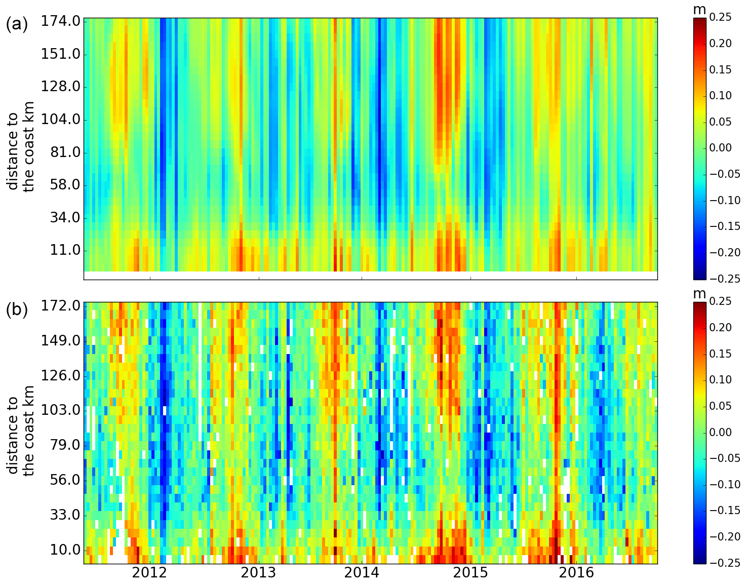
Figure 6 Hovmöller diagrams of SSH along the Jason-2 track 222 for the model (a) and for Jason-2 (b) as a function of the distance to the coast over the period 27 May 2011–1 October 2016.

4.2 The altimetry-data-filtering issue

In practice, users systematically apply a spatial filter to altimetry SLA data before geostrophic current derivation in order to remove the measurement noise observed in Sect. 4.1. The SLA filtering step is then a key element of altimetry current computation, and this is even more true in coastal areas. Consequently, the capability of altimetry to capture mesoscale currents depends on the choice of the filter.

Figure 6 illustrates this noise issue by presenting the Hovmöller diagrams of SSH derived from the model and from 1 Hz altimetry raw data along the Jason-2 track 222 in the 120 km close to the coast. Note that, with Jason-2, due to editing because of the noise, near-shore data are often missing. If the evolution of both SSH fields is globally similar, we clearly observe noise in altimetry data, as well as larger differences near the coast (i.e. in the first 30 km).

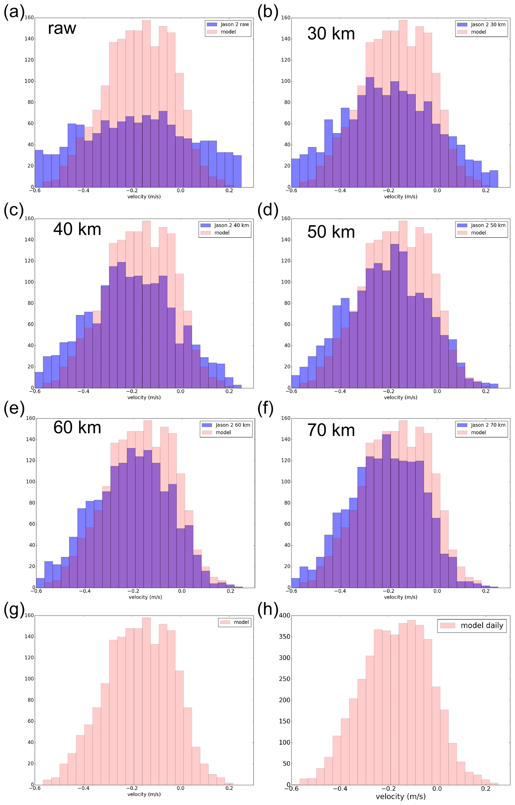
Figure 7 Distribution of the geostrophic current values along the Jason-2 track 222 and over the first 60 km to the coast over 27 May 2011–1 October 2016 for (a) raw altimetry data and (b), (c), (d), (e), (f) low-pass-filtered altimetry data with different cutoff frequencies indicated in the panels. Altimetry distributions (in blue) are superimposed on the corresponding model distribution (in pink). The latter is computed for the Jason-2 temporal resolution (g) and for the model resolution (h).

Table 4 Statistics corresponding to the distributions shown in Figs. 7, 8 and 9.

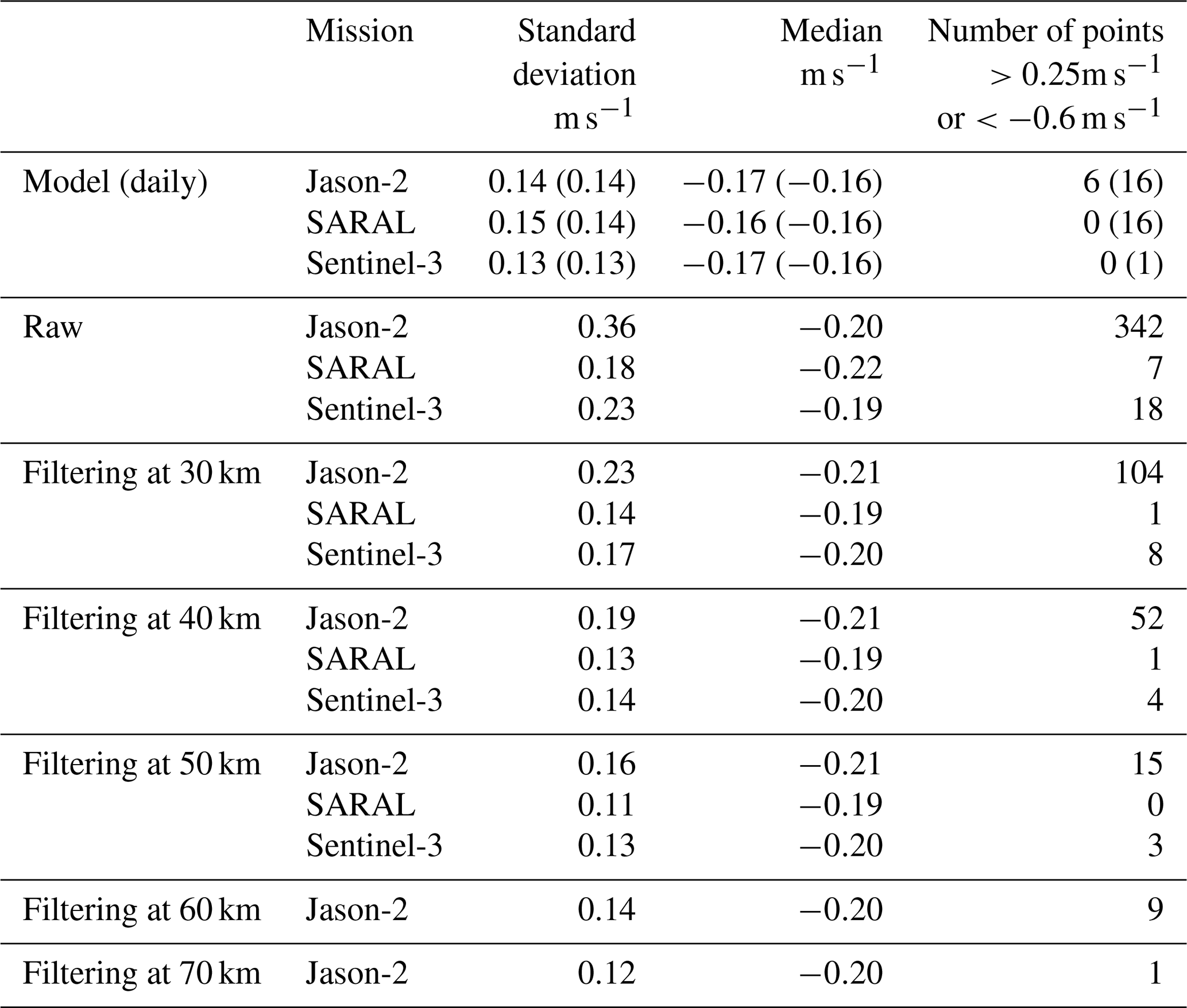
To estimate the best SLA filtering for the derivation of current estimates, we compute the distribution of the resulting geostrophic velocity values using raw and low-pass-filtered SLA altimetry data added to the MDT in the 60 km close to the coast. We compare the results to the distribution of the corresponding model velocities, used here again as a reference. To obtain the filtered SSH, we tested different cutoff frequencies on SLA data, ranging from 30 to 50 km for SARAL and Sentinel-3 and extending to 70 km for Jason-2, and then added the MDT. Indeed, Morrow et al. (2017) and Raynal et al. (2017) showed a greater noise level in Jason-2, which required larger cutoff frequency values. The histograms of current values are represented in Fig. 7 for Jason-2 track 222, in Fig. 8 for SARAL track 302 and in Fig. 9 for Sentinel-3 track 472 (altimetry in blue superposed on the model in pink). Note that, for each mission, the model current values are sampled at the altimetry temporal resolution (10, 35 and 27 d for Jason-2, SARAL and Sentinel-3 respectively) and at the model resolution to investigate the impact of undersampling data (bottom figures). Table 4 summarizes the statistics derived from the histograms, namely the median, the standard deviation and the number of points outside typical current values in this area, which are considered to be outliers (greater than 0.25 m s⁻¹ and smaller than −0.6 m s⁻¹ – these values are considered to be the typical NC velocities). Here, the distribution represents the variability of the current, and the objective is to be as close as possible to the current variability shown by the model.

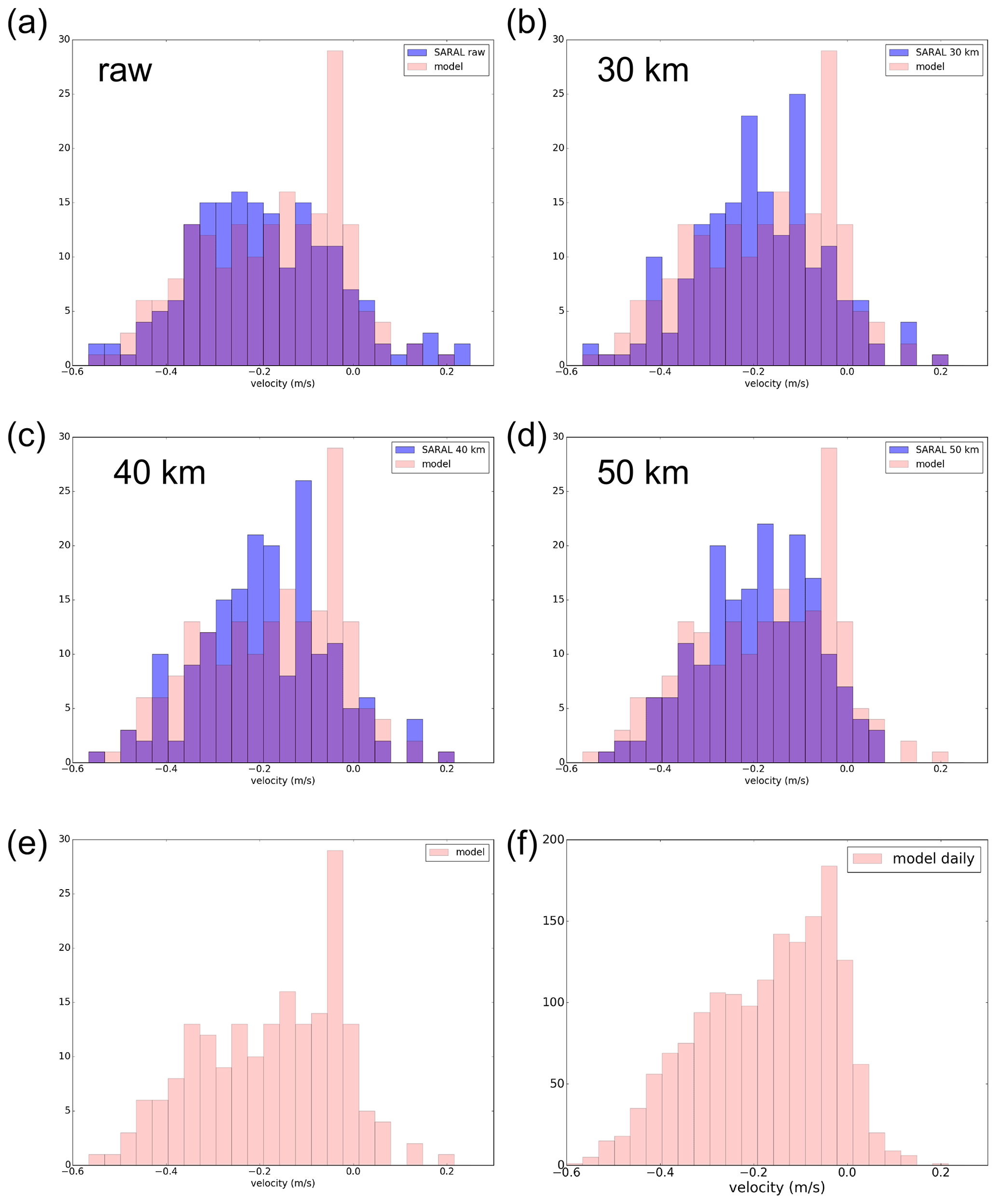
Figure 8 Distribution of the geostrophic current values along the SARAL track 302 and over the first 60 km to the coast over 24 March 2013–13 March 2016 for (a) raw altimetry data and (b), (c), (d), (e), (f) different filters indicated on each panel. The altimetry distribution (in blue) is superimposed on the corresponding model distribution (in pink). The latter is computed for the SARAL temporal resolution (g) and for the model resolution (h).

We first focus on Jason-2. The model reference shows a distribution which tends to be Gaussian. It is centred around −0.15 m s⁻¹, with a majority of negative values, and is slightly asymmetric. Jason-2 raw velocity values are almost randomly distributed. When Jason-2 SLA data are filtered, and as the cutoff wavelength increases, the histogram's distributions change and get closer to the model ones. Regarding the statistics (Table 4), the too-high standard deviation and too-negative median values in the raw Jason-2 data get closer to the reference with the increase in cutoff wavelength. With a 60 km filtering, we have the same standard deviation values in both Jason-2 and model velocities, but the median value always remains significantly lower in Jason-2. The number of outliers is also too large in raw Jason-2 data but decreases rapidly with the filtering; it is the closest to the model reference for a 60 km filtering. From these results, we conclude that Jason-2 currents tend to converge best towards the model reference with a filtering at 60 km. Beyond this cutoff wavelength, the smoothing erases the left- and right-hand sides of the distribution (Fig. 7) and reduces the variability.

We repeat the same analysis with SARAL (Fig. 8 and Table 4). Note that there are fewer satellite cycles for SARAL than for Jason-2, so less current data are available to compute statistics. As a result, the distributions obtained are more complex than for Jason-2. It is clearly observed when comparing Fig. 8e and f (distributions computed at the model resolution and at a 35 d resolution). The model histogram is initially centred on −0.07 m s⁻¹ with an asymmetric shape and a slight secondary peak around −0.25 m s⁻¹. When using the SARAL temporal resolution, the distribution is more random, with a peak around −0.07 m s⁻¹. The raw altimetry solution is less randomly distributed than for Jason-2, which is also confirmed by a standard deviation value 2 times smaller than for Jason-2 (0.18 m s⁻¹ vs. 0.36 m s⁻¹) and already relatively close to the 0.15 m s⁻¹ model reference. SARAL tends to converge towards the model with a filtering of 30 km.

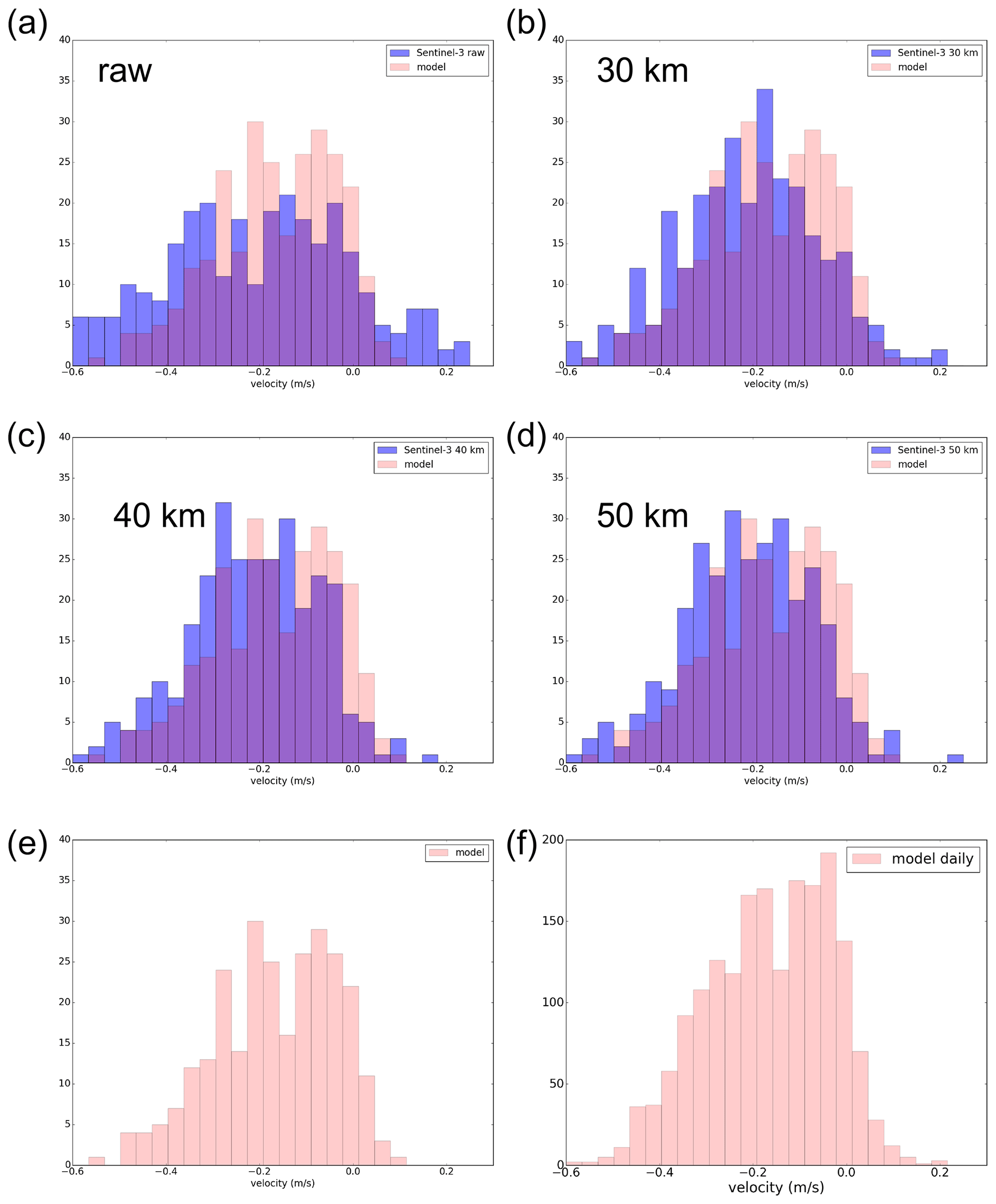
Figure 9 Distribution of the geostrophic current values along the Sentinel-3 track 472 and over the first 60 km to the coast for (a) raw altimetry data and (b), (c), (d), (e), (f) different filters (in blue). The altimetry distribution (in blue) is superimposed on the corresponding model distribution (in pink). The latter is computed for the Sentinel-3 temporal resolution (g) and for the model resolution (h). The Sentinel-3 distribution is over 18 June 2016–14 March 2019, and the model distribution is over 21 June 2014–15 March 2017.

For Sentinel-3, the distribution of the raw altimetry solution has a bimodal shape (Fig. 9a), as in the model. Its standard deviation is also largely closer to the model reference compared to Jason-2 (but slightly less than SARAL – Table 4). The statistics of the altimetry velocities tend to converge towards the model reference with a 40–50 km cutoff wavelength. One of the reasons for the slightly bimodal distribution in SARAL and Sentinel-3 may be the track orientation, which is quite different from the Jason-2 track which is perpendicular to the NC (Fig. 2e). Indeed, testing different track angles with the model reveals a small second peak (not shown).

Note that the values obtained in this study are slightly lower than the numbers given in Raynal et al. (2017), specifically ∼70 km for Jason-2 and 35–50 km for SARAL/AltiKa and Sentinel-3, even if these studies focused on open-ocean data. Morrow et al. (2017) also found values similar to Raynal et al. (2017) for the Jason-2 and SARAL missions through spectral analysis.

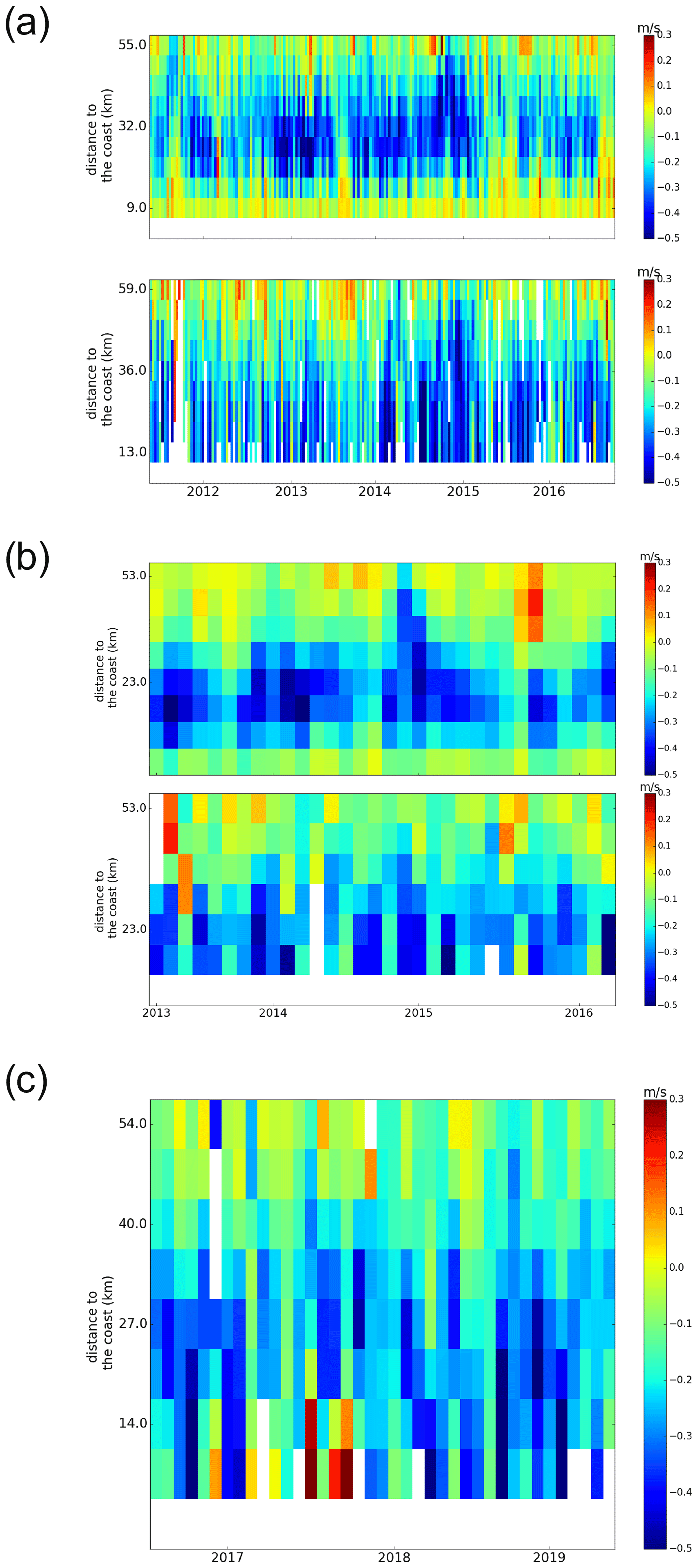
Figure 10 Hovmöller diagrams of the filtered across-track geostrophic current derived along the altimetry tracks for (a) Jason-2 track 222 over 27 May 2011–1 October 2016, (b) SARAL track 302 over 24 March 2013–13 March 2016 and (c) Sentinel-3 track 472 over 18 June 2016–14 March 2019. The corresponding model current is represented at the top panels of (a) and (b).

Figure 10 shows the Hovmöller diagrams of the geostrophic currents obtained after filtering with the optimal values found previously for each mission. Figure 10a along Jason-2 track 222 and Fig. 10b along SARAL track 302 include the model, as the period is the same, contrarily to Sentinel-3 (Fig. 10c). We focus on the first 60 km to the coast, as this corresponds to the NC. Figure 10a confirms that the NC is not fully resolved by Jason-2 (bottom panel). The model geostrophic current shown on the top panel indicates seasonal variations of the amplitude, width and location of the NC. These seasonal variations are partly reproduced by the filtered altimetry solution, especially for 2012 and 2013. In 2014, strong values in summer are visible in both the model and Jason-2.

The geostrophic currents derived from SARAL filtered data are shown in Fig. 10b in the bottom panel with the equivalent for the model in the top panel. Even with a less important filtering, SARAL data are less noisy. The seasonal pattern with stronger values in winter and weaker values in summer is very clear in the model and can also be seen in the altimetry. However, here again, the NC is not fully resolved due to the lack of the most coastal points.

By getting closer to the coast (Fig. 10c) Sentinel-3 data offer a more complete view of the NC, although some noisy values are found near the coast. The seasonal cycle is visible in 2017. However, with a repetitive cycle of 35 and 27 d respectively, SARAL and Sentinel-3 are less adapted to observation of these variations.

5 Summary and conclusion

In this study, we have presented a novel method to quantify the SSH signature of a narrow slope current, the NC in the NWMED, and to define its observability in altimetry data. It is based on a high-resolution numerical model, intensively validated against in situ glider and HF radar data and then considered as a reference for satellite altimetry data analysis. We consider the SSH and related surface geostrophic currents in parallel using three nadir-looking radar altimeters that employ different technologies, namely Jason-2, SARAL and Sentinel-3.

We show that, in the HF-radar-covered region, the NC has a clear signature in SSH, characterized by a sea level drop from offshore to the coast, generally centred at ∼15–20 km from the coast, with a mean value at 6.14^∘ E of 6.9 cm and spreading over 20 km. In winter, the SSH drops are generally stronger than in summer and are then theoretically easier for altimeters to detect. The NC is also clearly associated with high-frequency variability (Sect. 2.3 and 3). These results confirm that, as a narrow, variable and close-to-the coast current, the NC monitoring is an issue for satellite altimetry. It is also important to note here that, whatever the intrinsic performances of the instruments, the temporal resolution of the missions is an important limitation to the observation of coastal currents like the NC.“This point constitutes an advantage for Jason-2 in comparison to the SARAL and Sentinel-3 missions.

We then analyse the NC signature in altimetry data in comparison to the model reference. Jason-2 and SARAL 1 Hz data stop at 8 and 16 km from the coast respectively, sometimes preventing observation of the whole NC. Probably thanks to the SAR mode, it is better resolved in Sentinel-3, with data at 1 km from the coast. On average, the SSH drops associated with the NC are always overestimated in altimetry, with mean values that are 3.0 cm, 0.3 and 1.4 cm larger for Jason-2, SARAL and Sentinel-3 respectively. The mean NC core location is correctly located in Jason-2 and Sentinel-3, but it is slightly shifted in SARAL (8 km difference between the model and observations). In terms of current variability, all altimetry missions show much higher values than the model because of the measurement noise. However, this overestimation decreases significantly from Jason-2 (3.7 times larger) to the more recent Sentinel-3 and SARAL missions. The values closest to the model reference are obtained with SARAL (2.4 times larger against 2.9 for Sentinel-3). However, the noise remains too large, and all satellite SSH data must clearly be filtered before computing currents. By comparing the distributions of altimetry velocity fields derived with different filtering strategies with the model reference, we find that the optimal cutoff wavelength is 60, 30 and 40–50 km for Jason-2, SARAL and Sentinel-3 SSH data respectively.

In summary, to ideally address the coastal-observability question, future altimetry missions should combine instrumental improvements (Ka-band and SAR altimetry, as in SARAL and Sentinel-3) and the temporal resolution of Jason or better. Another approach would be to better optimize the use of data from the nine missions flying simultaneously in 2021.

The method presented here can be easily transposed to other altimetry missions and other dynamical processes apart from the NC. As an example, we could also focus on eddy observability, studying the size, amplitude and spatial configuration of their signature in SSH in comparison to the model reference. Using a carefully calibrated high-resolution model as a reference for coastal altimetry studies allows us to overcome the scarcity of independent observations to validate near-shore altimetry data. Models can be used as a reference to compare the performance of different altimetry missions but also of different coastal-data-processing strategies. They also provide 3D information on the whole range of ocean parameters that can be related to the sea level variations captured by altimetry.