the Creative Commons Attribution 4.0 License.
the Creative Commons Attribution 4.0 License.
 | 11 May 2023
Origins of mesoscale mixed-layer depth variability in the Southern Ocean
Igor Kamenkovich
Natalie Perlin
Mixed-layer depth (MLD) exhibits significant variability, which is important for atmosphere–ocean exchanges of heat and atmospheric gases. The origins of the mesoscale MLD variability in the Southern Ocean are studied here in an idealised regional ocean–atmosphere model (ROAM). The main conclusion from the analysis of the upper-ocean buoyancy budget is that, while the atmospheric forcing and oceanic vertical mixing, on average, induce the mesoscale variability of MLD, the three-dimensional oceanic advection of buoyancy counteracts and partially balances these atmosphere-induced vertical processes. The relative importance of advection changes with both season and average MLD. From January to May, when the mixed layer is shallow, the atmospheric forcing and oceanic mixing are the most important processes, with the advection playing a secondary role. From June to December, when the mixed layer is deep, both atmospheric forcing and oceanic advection are equally important in driving the MLD variability. Importantly, buoyancy advection by mesoscale ocean current anomalies can lead to both local shoaling and deepening of the mixed layer. The role of the atmospheric forcing is then directly addressed by two sensitivity experiments in which the mesoscale variability is removed from the atmosphere–ocean heat and momentum fluxes. The findings confirm that mesoscale atmospheric forcing predominantly controls MLD variability in summer and that intrinsic oceanic variability and surface forcing are equally important in winter. As a result, MLD variance increases when mesoscale anomalies in atmospheric fluxes are removed in winter, and oceanic advection becomes a dominant player in the buoyancy budget. This study highlights the importance of oceanic advection and intrinsic ocean dynamics in driving mesoscale MLD variability and underscores the importance of MLD in modulating the effects of advection on upper-ocean dynamics.
- Article
(8105 KB) - Full-text XML
- BibTeX
- EndNote


Mixed layer depth (MLD) changes drastically with time and location in the global ocean. Particularly large changes have been found in the northern part of the Antarctic Circumpolar Current (de Boyer Montégut, 2004; Dong et al., 2008; Sallée et al., 2010b). This MLD variability can be important for several reasons. The interannual variability of air–sea fluxes of oxygen and carbon dioxide in the Southern Ocean is primarily driven by changes in the entrainment of carbon-rich, oxygen-poor waters into the mixed layer during winter convection episodes (Verdy et al., 2007). Gaube et al. (2013) found that eddy-induced Ekman upwelling is at least partially responsible for sustaining positive phytoplankton anomalies in anticyclonic eddies of the South Indian Ocean, where intensified mixing homogenises chlorophyll throughout the winter-time mixed layer, which then enables satellite observations to detect a response to eddy-induced Ekman pumping in anticyclones. Mixed-layer dynamics also modulate the anomalous chlorofluorocarbon uptake by mesoscale eddies in the Drake Passage region (Song et al., 2015), as well as the seasonal variation in the correlation between anomalies of sea level and chlorophyll in the Antarctic Circumpolar Current (ACC) (Song et al., 2018). The oceanic mixed layer is also an important climatic variable, and the accuracy of MLD representation is crucial for closing the mixed-layer heat budget (Dong et al., 2007). MLD can modulate the air–sea thermal coupling by changing the upper-ocean heat inertia; specifically, a shallower (deeper) MLD makes the effective heat capacity lower (higher), and thus the sea surface temperature (SST) is more (less) sensitive to the surface heat flux (Tozuka and Cronin, 2014). As a result, the contribution of surface heat fluxes to surface frontogenesis and frontolysis depends not only on the gradients of the fluxes but also on the distribution of MLD (Tozuka et al., 2018). Therefore, understanding the origins of MLD variability in the Southern Ocean is important for studies of the oceanic biogeochemical processes, upper-ocean heat budget and air–sea thermal coupling. In this study, we will focus on the mechanisms of mesoscale MLD variability and their relations to atmospheric forcing.
Large-scale MLD variability is traditionally attributed to vertical mixing and convection, described by a one-dimensional process (Kraus et al., 1967). Within this framework, several previous observational studies have considered the relative importance of surface buoyancy forcing and wind-induced mixing in the mixed-layer formation (Dong et al., 2007, 2008; Sallée et al., 2010a; Downes et al., 2011; Holte et al., 2012; Sallée et al., 2021). For example, the scaling analysis in Sallée et al. (2010a) shows that the buoyancy forcing in the Southern Ocean dominates the wind mixing by 1 order of magnitude. In contrast, using two hydrographic surveys and a one-dimensional mixed-layer model, Holte et al. (2012) concluded that the wind-driven mixing is central to the winter-time formation of the Subantarctic Mode Water (SAMW), which has been associated with the mixed layer on the equatorward side of the ACC (Rintoul, 2002; Sallée et al., 2006; Holte and Talley, 2009). Holte et al. (2012) further demonstrated that the mixing driven by buoyancy loss and wind forcing is strong enough to deepen the SAMW mixed layer. This group of studies, however, neglected the role of the oceanic three-dimensional buoyancy advection, which can be an important player in the upper-ocean buoyancy budget and MLD variability. For example, using an eddy-resolving model in the Indo–western Pacific sector of the Southern Ocean, Li et al. (2016) found that, in regions with well-defined large-scale jets, there is a jet-scale overturning circulation with a sinking motion on the equatorward flank and a rising motion on the poleward flank of the jets. The authors suggested that this overturning is driven by the eddy momentum flux convergence rather than by Ekman pumping or suction and is thus a result of intrinsic oceanic variability. A follow-up study by Li and Lee (2017) considered a zonal-mean buoyancy balance and found that the downwelling branch of this overturning is responsible for the destratification underneath the mixed layer and therefore leads to the formation of the deep mixed layer north of the jets. Their study also concluded that the air–sea heat fluxes contribute to the large-scale mixed-layer formation along ACC fronts, while the Ekman advection only accounts for the destratification when the mixed layer initially deepens (Li and Lee, 2017).
Oceanic advection in MLD variability is likely to be more important at the mesoscale than at large scales. In this study, mesoscale anomalies are defined as anomalies on the spatial scales shorter than several oceanic Rossby deformation radii. At these spatial scales, the oceanic currents are particularly strong and highly variable and can be expected to dominate the upper-ocean heat and buoyancy budgets (Tamsitt et al., 2016; Small et al., 2020; Gao et al., 2022a). This study will explore the origins of MLD variability using an idealised atmosphere–ocean model of a sector in the Southern Ocean. The purpose of the study is to answer the following scientific questions: (1) what is the role of oceanic buoyancy advection in the mixed-layer dynamics and MLD variability? (2) What is the role of the surface buoyancy forcing and wind-induced mixing in the mixed-layer dynamics and MLD variability? (3) How do the upper-ocean state and MLD variability depend on the mesoscale air–sea coupling?
The first part of the study will analyse the upper-ocean buoyancy budget and focus on the relative importance of buoyancy advection in mesoscale MLD variability. In the second half of this paper, we examine how the mesoscale surface heat and momentum fluxes affect the MLD variability using two sensitivity experiments with modified atmosphere–ocean coupling. These flux anomalies can influence the mixed-layer variability through buoyancy forcing and wind-driven mixing (Kraus et al., 1967; Dong et al., 2007, 2008; Sallée et al., 2010a; Downes et al., 2011; Holte et al., 2012; Sallée et al., 2021), and we will explore the relative importance of these effects. The flux variability can be driven by SST anomalies because air–sea heat exchanges act to damp SST anomalies (Putrasahan et al., 2013; Gao et al., 2022a). Additionally, acceleration (deceleration) of surface winds over warm (cold) SST anomalies modulate the turbulent air–sea heat exchange (Xie, 2004; Small et al., 2008), which may be important when winds are strong. These fluxes can also result from internal atmospheric dynamics, but we will not attempt to study the intrinsic and SST-forced sources of flux variability separately.
2.1 Regional ocean–atmosphere model and sensitivity experiments
The regional ocean–atmosphere model (ROAM) is a semi-idealised, high-resolution regional coupled model. Here, we provide a brief description of the model, since it is described in greater detail by Gao et al. (2022a) and Perlin et al. (2020). The atmospheric component is the US Navy Ocean–Atmosphere Mesoscale Prediction System (Hodur, 1997), forced by lateral boundary conditions from the global reanalysis dataset. The global reanalysis dataset is derived from a 6-hourly 0.25∘ global NCEP (National Centers for Environmental Prediction) FNL (Final) analysis and Global Forecast System (GFS). The atmospheric component has the following two nested domains: the inner domain that is fully coupled with the ocean component and the outer domain that is one-way coupled with the observed SST. The inner and outer atmospheric domains have 9 and 27 km horizontal grid box sizes, respectively; both domains have 49 vertical layers. The transition between the inner and outer domains uses a blending scheme that ensures a gradual transition between Regional Ocean Modeling System (ROMS)-simulated SST and observed SST surrounding the ocean grid. The ocean component is the Regional Ocean Modeling System (ROMS) (Shchepetkin and McWilliams, 2005), formulated in a zonal re-entrant channel with north and south sponge boundaries that help to keep the meridional density gradient close to a desired value. The atmospheric forcing at the sea surface comes from the atmospheric component. The horizontal ocean grid box is 2.5 km, and there are 30 sigma layers in the vertical. The channel is 2800 km long and 1120 km wide. The large-scale stratification in the ocean is chosen from a region in the western Indian sector of the Southern Ocean. The domain and bathymetry are shown in Fig. 1 in Gao et al. (2022a). The one-day snapshot of SST, eddy kinetic energy (EKE) and MLD (Fig. 1a–c) reveals transient mesoscale structures, including a predominantly eastward flow with a strong jet in the northern part of the domain, as shown in Fig. 1d. Mesoscale anomalies are evident in all fields displayed in Fig. 1. Figure 6f of Perlin et al. (2020) illustrates deeper MLD formation in the northern flank of the ACC in the southern Indian sector.

Figure 1Examples of model-simulated fields (values on 1 September 2016): (a) sea surface temperature, (b) eddy kinetic energy, (c) mixed-layer depth (MLD), (d) surface ocean current speed, (e) downward sea surface heat fluxes and (f) surface wind stress.
In addition to the control simulation, we carried out the following two sensitivity experiments: the smooth-heat-flux experiment and the smooth-momentum-flux experiment, in which the mesoscale air–sea heat fluxes (turbulent and radiative components) and wind stress respectively are removed with spatial smoothing by a 300 km by 300 km running boxcar average. Wind stress is calculated from the model friction velocity and 10 m wind directional components (Perlin et al., 2020) and is not calculated relative to surface current. The control and sensitivity experiments are spun up for 3 years, following a 12-year spin-up of the uncoupled ocean model. The length of the spin-up is deemed to be sufficient to reach equilibrium for the upper-ocean temperature based on the equilibrium of the domain-average eddy kinetic energy. The control and the sensitivity experiments are then run for 2 more years using the atmospheric lateral boundary conditions from July 2015 to June 2017. Although the duration of the simulations is relatively short, the main analysis is based on relations within numerous mesoscale features, which will ensure that the conclusions are statistically significant.
2.1.1 Ocean mixed-layer buoyancy budget
We diagnose spatial and temporal variations in the upper-ocean buoyancy budget here in order to examine the origins of the MLD variability. Following Li and Lee (2017), the depth-dependent buoyancy budget can be expressed as
where is buoyancy, g represents the gravitational acceleration, δσ is the potential density anomaly, ρ0=1027 kg m−3 is the reference density, u is the three-dimensional velocity vector, αθ is the thermal expansion coefficient, βS is the haline contraction coefficient, θ is the potential temperature, S is the salinity, D(θ) is the potential temperature diffusion, D(S) is the salinity diffusion, and the buoyancy forcing term B is
where Cp=3850 J (kg C)−1 is the specific heat of seawater, and q is the downward shortwave radiation (units W m−2). At the ocean surface, the downward surface heat fluxes can be decomposed into the following four components:
where QSW is the shortwave radiation, QLW is the longwave radiation, Qs is the turbulent sensible heat flux, and Ql is the turbulent latent heat flux.
In order to examine the evolution of the vertical stratification in the upper ocean, we take the vertical derivative () of the buoyancy and compute the buoyancy frequency squared (N2) as follows:
As a measure of stratification, N2 is positive, corresponding to a stable water column. Taking the vertical derivative of Eq. (1) and combining it with Eq. (4), we can get the depth-dependent buoyancy frequency budget as follows (Li and Lee, 2017):
The first term on the right-hand side quantifies the re-stratifying effect of advection on the water column. Its positive values indicate that advection increases the stratification and hydrostatic stability. In order to emphasise the net effect of all processes on the MLD, we integrate Eq. (5) in the vertical to get the buoyancy frequency budget over the mixed layer as follows:
where H is the MLD, defined here as the depth at which the potential density increases by 0.03 kg m−3 relative to the surface value. The mixed-layer integrated tendency term indicates whether the mixed layer as a whole is becoming more or less stratified. The advective term is now in the form of the difference between surface buoyancy advection and advection at the base of the mixed layer. Its positive values indicate that the advection acts to shoal the mixed layer. If the buoyancy advection increases the buoyancy difference between the surface and the base of the ML, this term has a re-stratifying tendency, and the mixed layer shoals. If the buoyancy advection decreases the buoyancy difference between the surface and the base of the mixed layer, this term has a destratifying tendency, and the mixed layer deepens.
The residual term represents the contribution of the atmospheric buoyancy forcing and oceanic subgrid mixing. These processes are related, since surface heat exchanges are associated with changes in stratification, vertical mixing and convection, whereas stronger momentum fluxes lead to intensification of mixing. The atmospheric forcing is, thus, implicit in the vertical mixing term, and its direct role in the budget is difficult to quantify. We will not attempt to do it in our analysis. The residual term also includes diffusion and cabling terms due to nonlinear effects (Li and Lee, 2017). These buoyancy budget terms are calculated from daily snapshots of the model output in order to minimise sampling errors.
We begin by exploring the one-dimensional view on the mixed-layer deepening and shoaling, which implies that variations in MLD are primarily caused by changes in surface density. The large-scale MLD is indeed well correlated with the SST (correlation coefficient is −0.7), with a cooler (warmer) SST leading to deeper (shallow) MLD. In contrast, the relationship becomes more complicated for mesoscale anomalies, which are defined as departures from the 300 km by 300 km running boxcar average. Here we use eddy and mesoscale anomalies interchangeably, but eddies, in our definition, do not solely mean coherent vortices but also include fronts, waves and jets. The mesoscale MLD and SST anomalies are only weakly correlated, with the average correlation coefficient of −0.2 (Fig. 2). The relatively weak correlation can be explained by the importance of oceanic advection in MLD variability, which will be explored in the following sections.
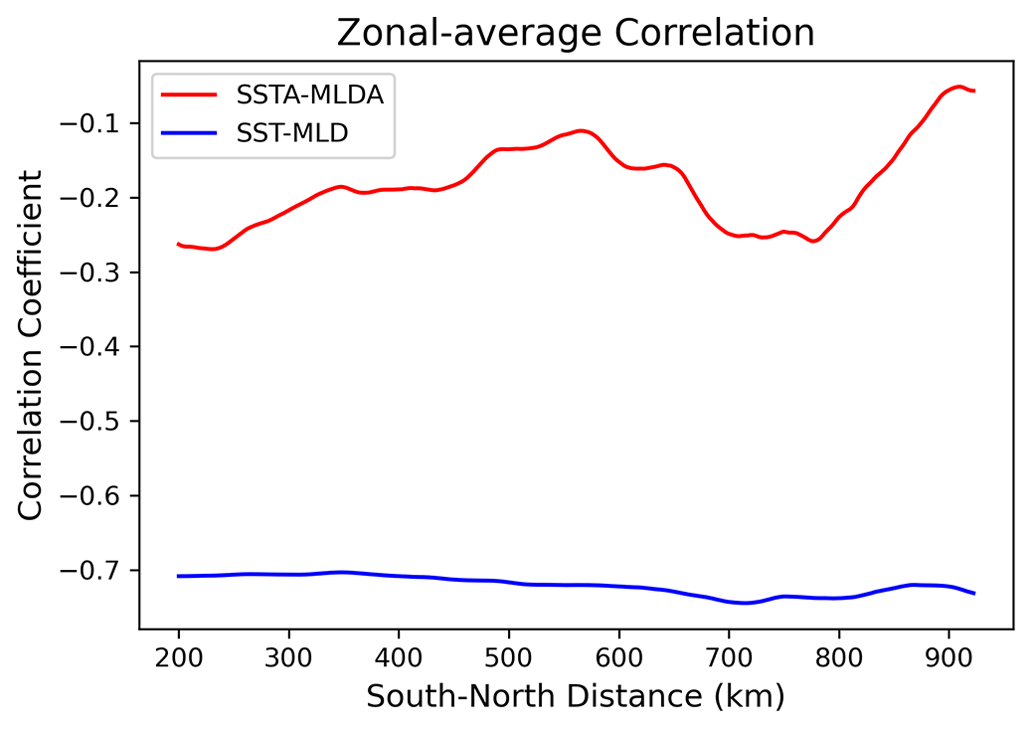
Figure 2Zonally averaged correlation coefficient between SST and MLD (blue line) and zonally averaged correlation coefficient between SST and MLD anomalies (red line). The anomalies are defined as the departure from the 300 km by 300 km running boxcar average.
3.1 Mixed-layer buoyancy balance
We first examine the monthly depth-dependent buoyancy budget at the depth–latitude cross-section taken at X=2000 km in the zonal direction in order to identify the key processes that contribute to the seasonal variability in MLD. We also examined section X=1000 km and reached the same conclusion. The evolution of the upper-ocean stratification and hydrostatic stability is measured by the tendency in the buoyancy frequency squared (N2) – see Eq. (5). From January to March, the positive N2 tendency (re-stratifying signal) at the base of the mixed layer indicates that the water column gets more stable during the warm summer months (Fig. 3a). The mixing and atmospheric forcing (residual) term makes the largest contribution to the N2 tendency everywhere within the mixed layer and is spatially correlated with the tendency (Fig. 3b). The buoyancy advection has a re-stratifying effect over most of the mixed layer, but it is not spatially correlated with the N2 tendency (Fig. 3c).
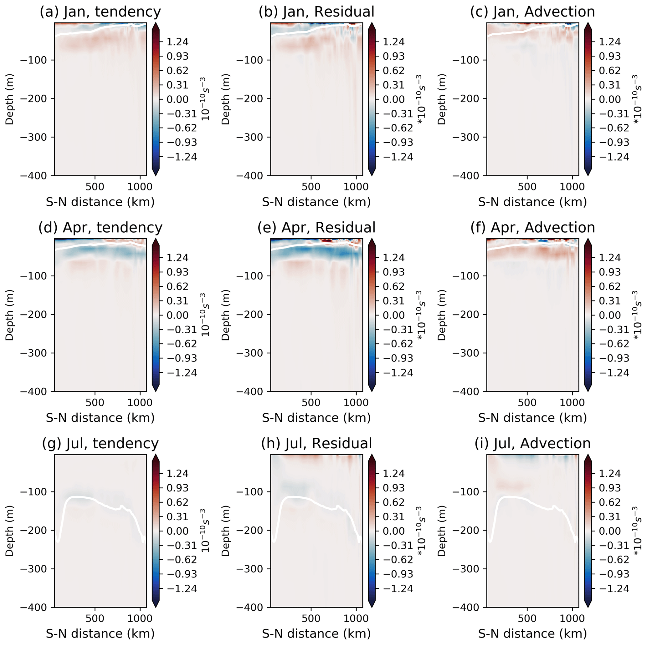
Figure 3Monthly mean depth-dependent buoyancy budget in the control case at the vertical cross-section X=2000 km in January, April and July, respectively. (a, d, g) N2 tendency (shading; unit: s−3) and MLD (white line; unit: metres), (b, e, h) residual term (shading; unit: s−3) and MLD, and (c, f, i) buoyancy transport contribution term (shading; unit: s−3) and MLD.
Starting in April, the N2 tendency turns negative at the mixed-layer base, which indicates that the water column is getting less stable and that the mixed layer is beginning to deepen (Fig. 3d). From May to August, the N2 tendency is negative around the mixed-layer base, which indicates that the mixed layer continues to deepen, consistent with the destratifying effects of the austral winter-time surface cooling (Fig. 3g). The destratifying effects as a result of the mixing and atmospheric forcing explain most of the N2 tendency around the base of the mixed layer (Fig. 3e, h). The advective restratification term stays positive, which implies that the buoyancy advection acts to shoal the mixed layer (Fig. 3f, i).
In September, the N2 tendency is nearly zero, while the mixed layer is the deepest (Fig. 4a). The mixing and atmospheric forcing (residual) term (Fig. 4b) continues to destratify the mixed layer, but these effects are now very small everywhere, except near the surface, where they are compensated for by the buoyancy advection (Fig. 4c). The advective term is also very small in most of the domain (Fig. 4c). In December, the N2 tendency turns mostly positive at the base of the mixed layer (Fig. 4g), meaning that the water column is re-stratifying, which leads to the shoaling of the mixed layer. In December, the destratifying effect of the residual term in the upper 80 m is compensated for by the restratification (Fig. 4h–i), and the tendency is very weak within the mixed layer.
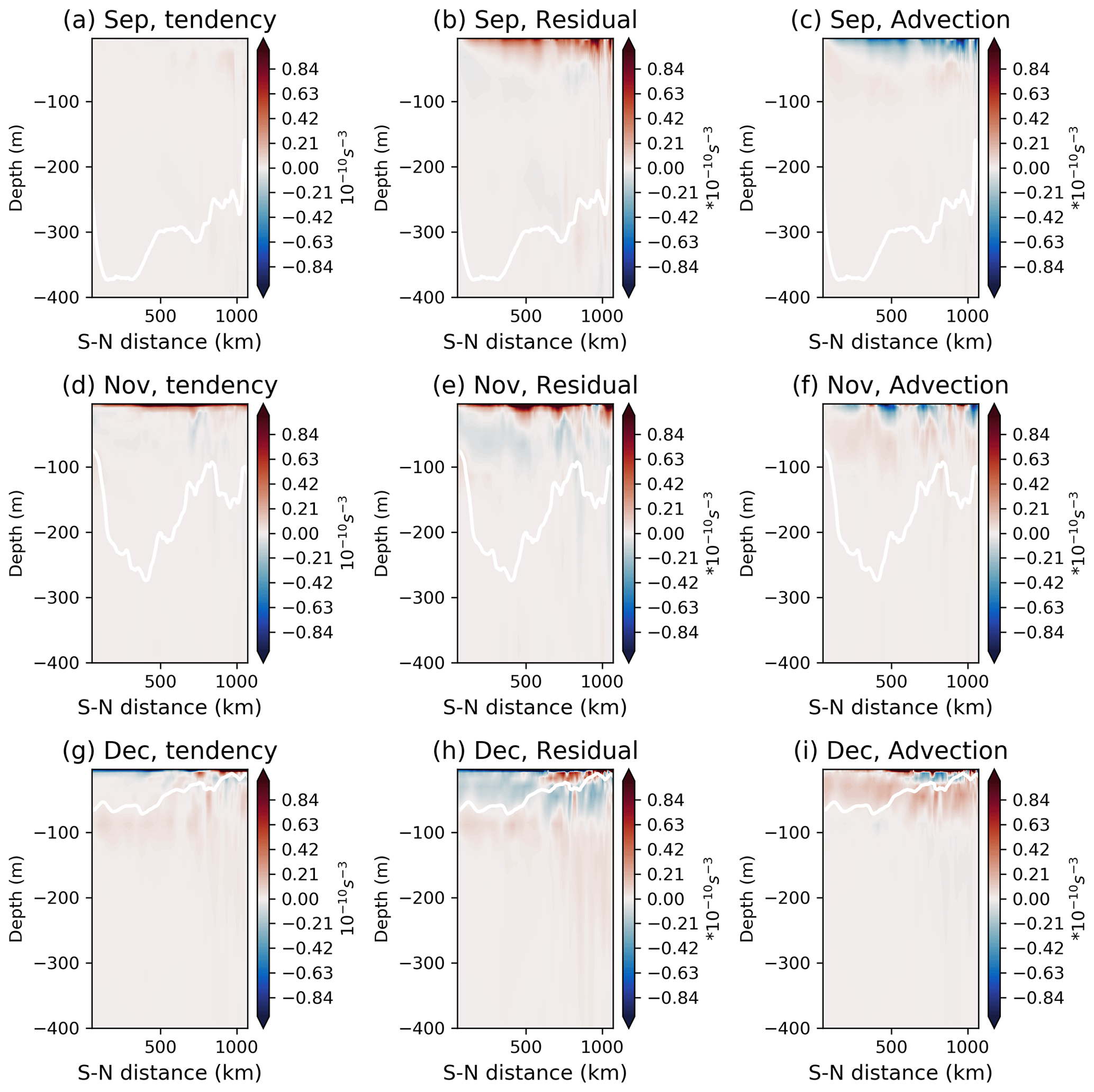
Figure 4Monthly mean depth-dependent buoyancy budget in the control case at the vertical cross-section X=2000 km in September, November and December, respectively. (a, d, g) N2 tendency (shading; unit: s−3) and MLD (white line; unit: metres), (b, e, h) residual (shading; unit: s−3) term and MLD, and (c, f, i) buoyancy transport contribution term (shading; unit: s−3) and MLD.
Next, we present the depth-integrated monthly mixed-layer buoyancy budget in Eq. (6). The advantage of this analysis is that it allows us to focus on the lateral mesoscale structure in all budget terms. From January to March (austral summer), when the MLD is relatively shallow, the evolution of the vertical density contrast (integrated N2 tendency) is caused by the atmospheric forcing and ocean mixing (Fig. 5a–b). The advection term is much smaller than the residual term, except in the jet region (Fig. 3), where it exhibits small-scale anomalies with the spatial scale of O[10 km] (Fig. 5c). These anomalies are persistent throughout the year in the jet region. Note that, despite the importance of short spatial scales, the dynamics everywhere in the domain are still geostrophic, since we verified that the Rossby number, measured by a ratio between the relative and planetary vorticity, is small. In June, when the mixed layer is deepening, the advection and residual terms are both large and tend to balance each other in the southern part of the domain (Fig. 5e–f). In September, when the MLD reaches its maximum, the advection and residual terms balance each other, and the tendency term is small (Fig. 5g–i). From September to December, both the advection and residual continue to play equally important roles in the buoyancy budget.
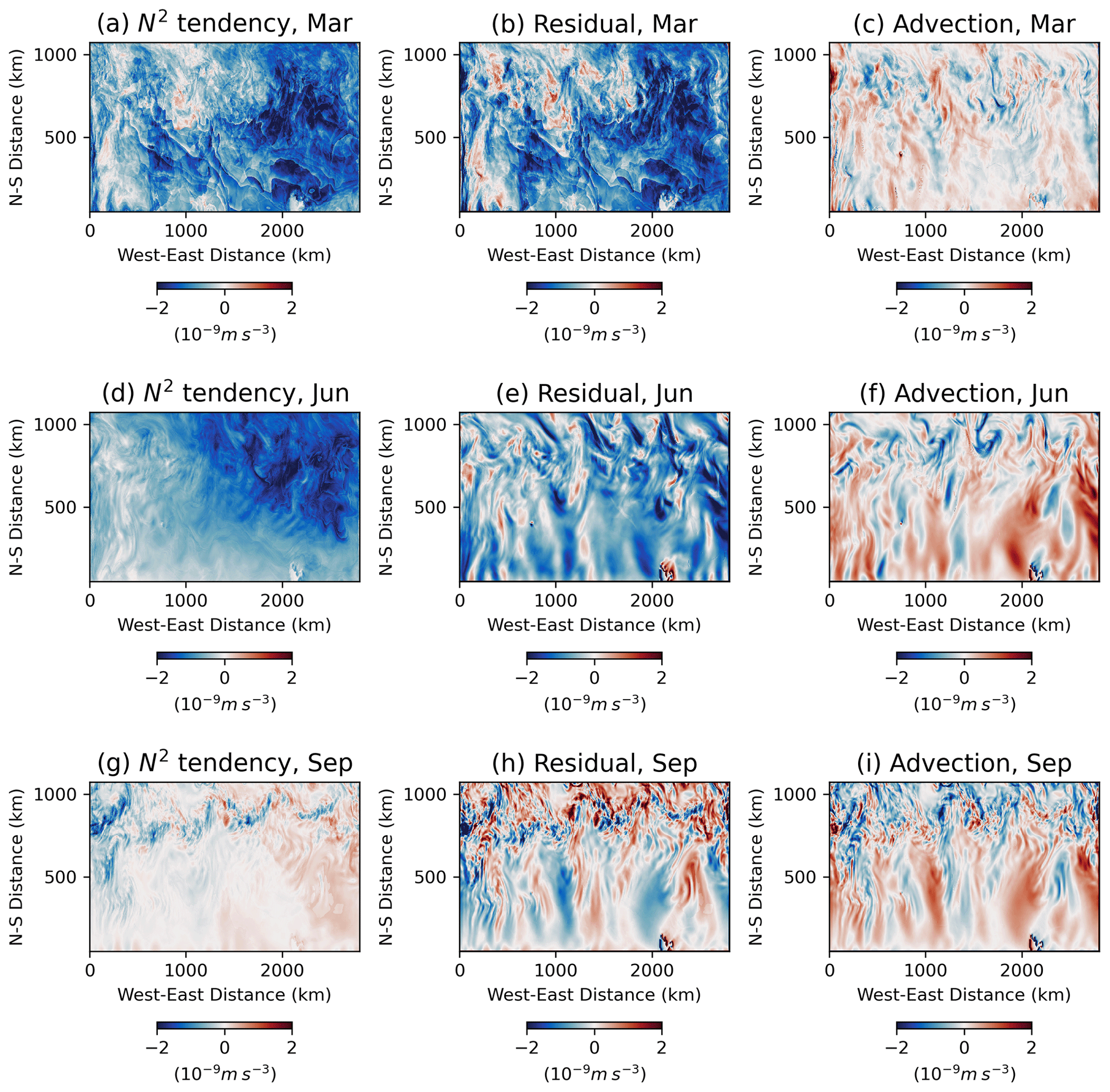
Figure 5Monthly mean mixed layer-integrated buoyancy budget in the control case in March, June, and September 2016: (a, d, g) N2 tendency, (b, e, h) residual term and (c, f, i) buoyancy transport contribution term in Eq. (6) (unit: m s−3).
In summary, both buoyancy advection and residual processes (mixing and atmospheric forcing) play important roles in MLD variations. There is, however, significant seasonality in the buoyancy budget. The mixing and atmospheric forcing are the dominant terms in summer and autumn (January to May), when they drive variations in MLD, while the buoyancy advection becomes equally important in winter and spring (from June to December). In late winter, the advection balances the mixing and atmospheric forcing. The MLD modulates the relative importance of advection, with the thicker and more thermally inert mixed layer being less controlled by the atmospheric forcing. Another important result is that buoyancy advection by ocean eddies can have both re-stratifying and destratifying effects, whereas some previous studies only account for their overall re-stratifying effect (Fox-Kemper et al., 2008; Fox-Kemper and Ferrari, 2008).
3.2 Mixed-layer response to mesoscale atmospheric forcing
The results so far have demonstrated the importance of both atmospheric forcing and oceanic buoyancy advection in driving mesoscale MLD variability. The conclusions were, however, drawn from spatial relations between the corresponding terms in the buoyancy budget, which is not sufficient for quantifying contributions from each process in such a highly nonlinear system. For example, in addition to directly affecting the stability of the upper ocean, the mesoscale atmospheric forcing can also influence buoyancy advection and oceanic mixing. The sensitivity experiments described in this section will directly inquire about the role of atmospheric heat and momentum fluxes in the corresponding dynamics.
Downward heat fluxes and wind stress at the sea surface in the control experiment exhibit well-pronounced mesoscale variability (Fig. 1e–f). As is discussed in the Introduction, this variability is both a result of internal atmospheric variability and a response to mesoscale SST anomalies. In the smooth-heat-flux and smooth-momentum-flux experiments, we remove these mesoscale anomalies in the air–sea heat fluxes and wind stresses respectively using a 300 km by 300 km moving average. This is done during coupling, so the ocean model is forced by either the large-scale heat fluxes or wind stresses.
The zonal-mean structure of the surface heat flux and wind stress in the control, smooth-heat-flux and smooth-momentum-flux experiments are very close to each other (within 10 % or less, not shown). Mesoscale heat flux anomalies are particularly large in the jet region in the northern part of the domain (not shown). In the control experiment, the turbulent heat fluxes are negatively correlated with SST anomalies, and this negative relationship is stronger in the northern domain where the ocean currents themselves are stronger (Fig. 6a). This negative correlation indicates that the mesoscale air–sea heat fluxes dampen the SST anomalies. As a result of smoothing out the mesoscale heat fluxes, the relationship between SST anomalies and turbulent heat fluxes is significantly weaker in the smooth-heat-flux experiment, indicating a reduced atmospheric feedback on SST anomalies (Fig. 6a).
In the smooth-momentum-flux experiment, the ocean does not feel the mesoscale wind stress anomalies, which are mainly a response to SST variability (Perlin et al., 2020). Specifically, mesoscale wind stress is positively correlated with SST anomalies in the control experiment, and this relationship is stronger in the northern part of the domain, where the ocean currents are stronger (Fig. 6b). A positive correlation indicates that the wind stress is stronger (weaker) over warm (cold) SST anomalies. Wind stress variability, in turn, induces anomalous Ekman circulation. As a result of smoothed-out mesoscale wind stress anomalies, the relationship between SST anomalies and wind stress is significantly weaker in the smooth-momentum-flux experiment (Fig. 6b). The effects on the SST variability itself are, however, weaker than in the smooth-heat-flux case.
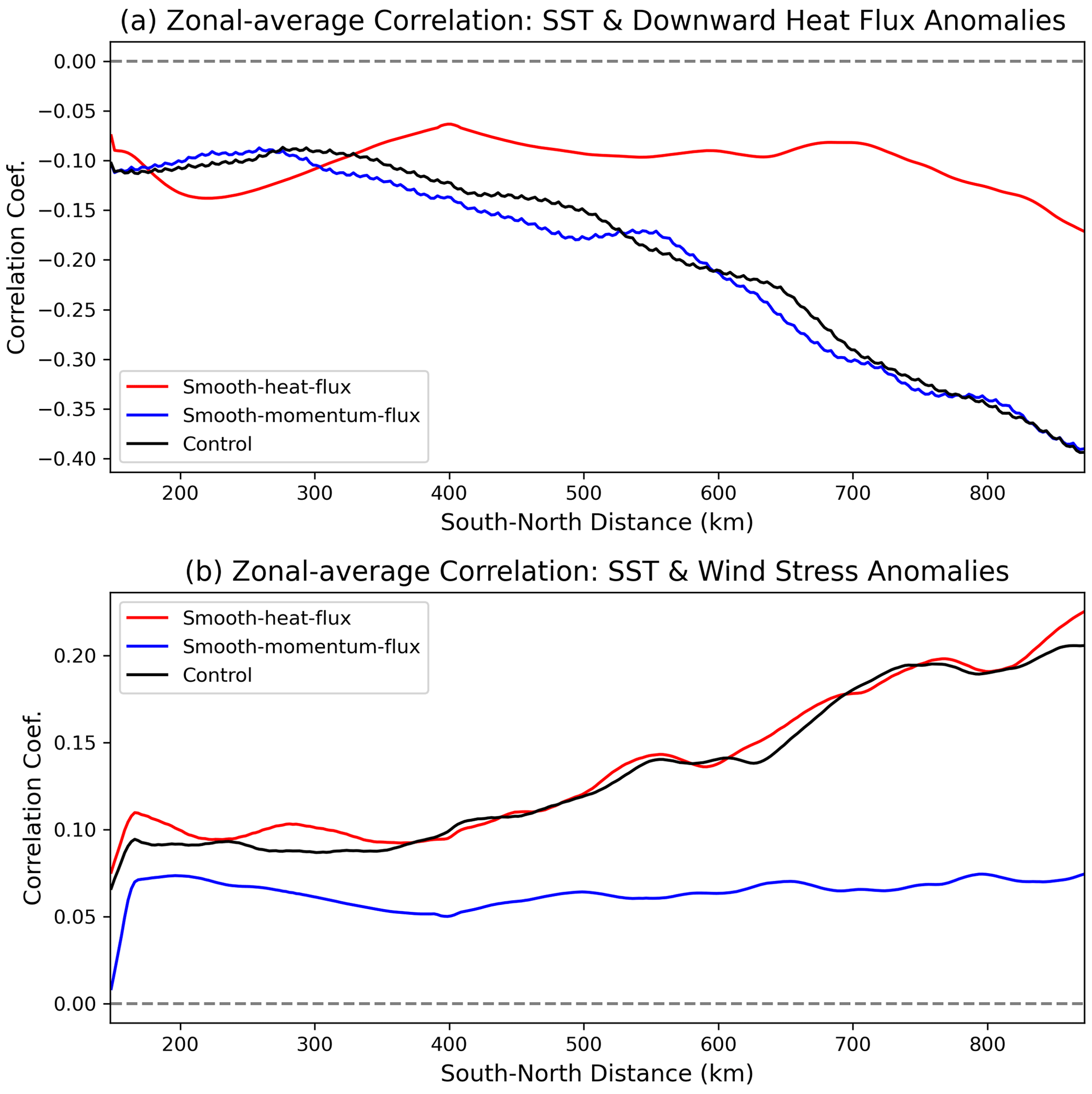
Figure 6(a) Zonally averaged correlation coefficient between mesoscale SST anomalies and turbulent heat flux anomalies; (b) zonally averaged correlation coefficient between SST anomalies and sea surface momentum stress. The control case is shown by the green line, and the smooth-heat-flux (Smooth-momentum-flux) case is shown by the red (blue) line.
As a consequence of the smoothing of atmospheric forcing, there are significant differences in mesoscale SST variability between the control and sensitivity experiments. The atmosphere feeds back on mesoscale SST anomalies via turbulent air–sea fluxes and wind stress. Smoothing of these fluxes weakens this feedback. For example, the lack of atmospheric thermal damping in the smooth-heat-flux case leads to the enhanced mesoscale SST variability from January to May, as shown in the domain-average root-mean-squared (rms) SST anomalies (Fig. 7). Note also that a part of mesoscale variability in surface heat and momentum fluxes is not an SST-forced response but is instead a result of intrinsic atmospheric variability.
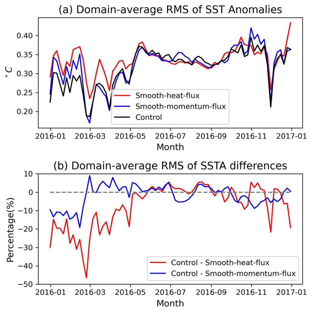
Figure 7(a) Time series of domain-averaged root-mean-squared (rms) SST anomalies in the control (black), smooth-heat-flux (red) and smooth-momentum-flux (blue) experiments; (b) time series of the domain-averaged differences in SST rms between the control run and smooth-heat-flux experiment (red line) and between the control run and smooth-momentum-flux experiment (blue line).
The rms mesoscale MLD anomalies exhibit noticeable differences (up to 20 %) between the control run and the sensitivity experiments (Fig. 8). Figure 8b shows the ratio between the rms of MLD between the simulations. From January to May, the results suggest that mesoscale air–sea heat fluxes enhance MLD variability because it decreases when the mesoscale surface fluxes are filtered out. During this time period, the MLD is shallow, and its variability is mainly driven by the atmospheric forcing and ocean vertical mixing (Fig. 5), and it is not surprising that the reduction in mesoscale surface heat and momentum fluxes leads to weaker MLD variations. From September to November (local spring), the opposite is true; the mesoscale MLD variability is weaker in the control case than in the sensitivity runs. This result may look counter-intuitive and deserves further discussion. During the local spring in the control experiment, the buoyancy advection is balanced by the mixing and atmospheric forcing in most of the domain (Fig. 5). This balance is characteristic of the thick mixed layer, with its high inertia. When one of the two main terms in this balance, the mesoscale surface flux, is artificially reduced in the sensitivity runs, the balance is no longer valid, and the MLD variability is enhanced. As briefly discussed in Sect. 2, the significance of the changes is guaranteed by a large number of mesoscale anomalies. In order to further test the robustness of the aforementioned conclusions, we calculated the same rms MLD anomalies in the western half, the eastern half and the northern half (which contains the jet region) subsets. We found, qualitatively, the same seasonality in all three subsets (not shown).
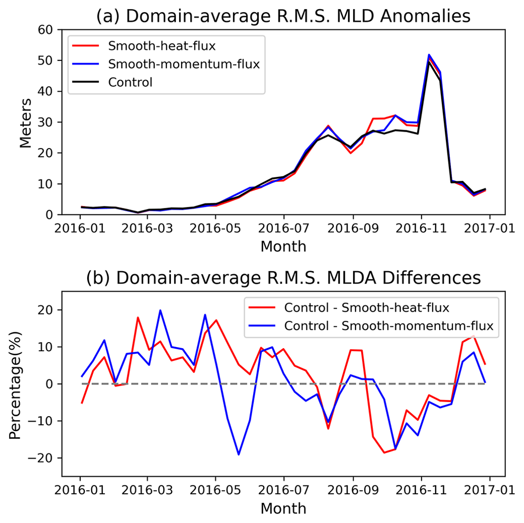
Figure 8(a) Time series of domain-average root-mean-squared (rms) MLD anomalies in the control (black), smooth-heat-flux (red) and smooth-momentum-flux (blue) experiment; (b) time series of the domain averaged rms MLD anomaly differences (in percentage) between the control run and smooth-heat-flux experiment (red line) and between the control run and smooth-momentum-flux experiment (blue line).
Compared to the mesoscale variability in MLD, the mesoscale atmospheric forcing makes a small difference (below 6 %) in the domain-average MLD (Fig. 9). The spatial distribution of the annual-mean MLD differences exhibits a dipolar structure, with a larger magnitude in the northern part of the jet region and smaller values in the southern part (not shown), which is similar to the annual-mean difference in the ocean current speed. The shape of the patterns and their similarity indicate a southward shift and suggest a relation between the jet and the meridional slope in the MLD. This conclusion is confirmed by the vertical cross-sections. The magnitudes of the changes are, however, small, and their significance is hard to evaluate.
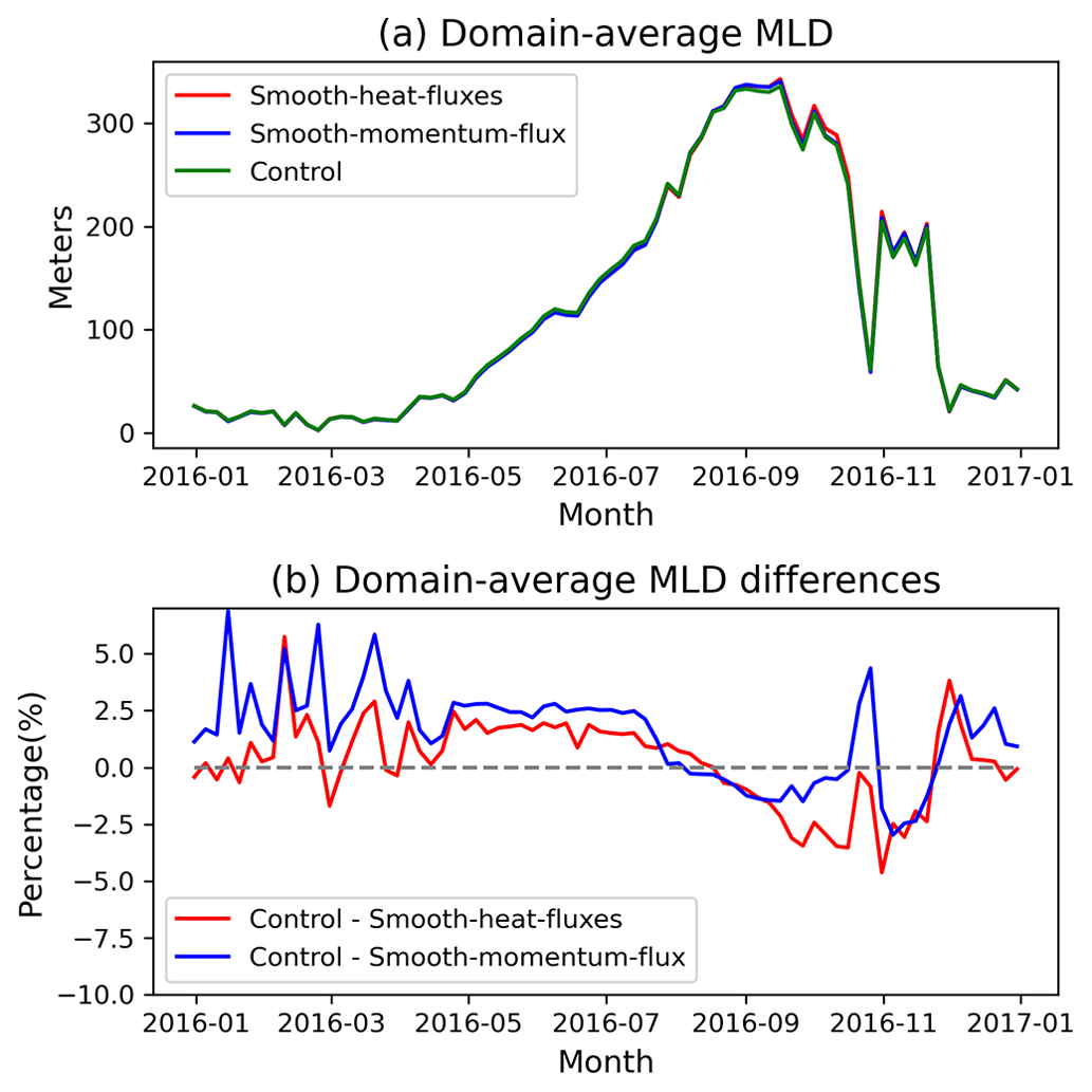
Figure 9(a) Time series of the domain-averaged MLD in the control (green), smooth-heat-flux (red) and smooth-momentum-flux (blue) experiments; (b) time series of the domain-averaged MLD differences between the control and smooth-heat-flux experiment, shown by the red line, and the difference between the control and smooth-momentum-flux experiments, shown by the blue line. (unit: metres)
The mixed layer in the Southern Ocean modulates ocean–atmosphere exchanges of heat and atmospheric gases by changing the effective upper-ocean thermal inertia. In this study, we explore the origins of MLD variability using both buoyancy budget analysis in ROAM simulations and sensitivity experiments. The results demonstrate that oceanic advection plays a central role in the buoyancy budget and that this role is amplified when the mixed layer is deep. The advection term in our analysis is composed of the following two parts: the locally forced Ekman advection driven by the wind and the geostrophic and ageostrophic processes that exhibit strong mesoscale variability. We expect the ageostrophic variability to be much weaker than the geostrophic part, since the Rossby numbers in the domain are much smaller than 1. The Ekman current, as part of the advection, is expected to play a role in regions with strong wind variability and SST gradients (Small et al., 2020; Gao et al., 2022a).
In the budget analysis, the time evolution of the buoyancy frequency N2 represents the re- or destratifying tendency in the water column. This tendency is driven by the following two main processes: the three-dimensional advection of buoyancy and the atmospheric forcing and upper-ocean mixing (the residual term). The mixing and surface fluxes of heat and momentum in the residual term are closely intertwined and represent the one-dimensional vertical forcing. The budget also exhibits strong seasonal variations due to the changes in mixed-layer heat inertia. In summer and autumn, when the mixed layer is shallow, atmospheric forcing and ocean mixing dominate the budget, while the buoyancy advection is of minor importance, and its significance is mainly restricted to the jet region. In winter and spring, when the mixed layer is deep and its inertia is large, the buoyancy advection becomes more important and balances the mixing and atmospheric forcing. Another important result is that the advection can have both re-stratifying (mixed-layer shoaling) and destratifying (mixed-layer deepening) effects. In fact, the destratifying advective effects are widespread at the mesoscale, which challenges a common view that mesoscale eddies always restratify the upper ocean.
The importance of mesoscale surface heat and momentum fluxes is directly addressed in two sensitivity experiments, the smooth-heat-flux and smooth-momentum-flux experiments. In the smooth-heat-flux experiment, the ocean component is forced with large-scale surface heat fluxes, whereas the atmospheric component still reacts to the full SST anomalies. Similarly, the ocean component in the smooth-momentum-flux experiment is forced by large-scale surface wind stress. For the mesoscale MLD variability, there is seasonal variation in the importance of mesoscale atmospheric forcing, which is consistent with our conclusions from the budget analysis. The atmospheric forcing dominates the summer-time mesoscale buoyancy budget in the control simulation, and the absence of mesoscale heat and momentum fluxes leads to smaller MLD anomalies in the sensitivity runs. In winter, there is a balance between the buoyancy advection, mixing and atmospheric forcing in the control simulation, and variations in water column stability are small. The reduction in the variability of the atmospheric forcing in the sensitivity experiments breaks this balance and leads to the enhanced advection-driven variability in MLD. Seasonal variations are a significant factor in the RMS MLD anomaly variability and its response to atmospheric forcing at the mesoscale, regardless of whether this forcing is due to heat or momentum fluxes. Specifically, during the summer season, the MLD is shallower, and the atmospheric forcing is typically more influential. Conversely, during winter, the MLD is deeper and has higher inertia, and atmospheric forcing is generally less critical.
This study explores the regime of mesoscale atmosphere–ocean coupling, which is important for the upper-ocean dynamics and mixed-layer variability. The mixed-layer variability has implications for both physical and biochemical processes in the Southern Ocean. The findings demonstrate the tendency of atmospheric forcing and advection to compensate for each other in the mixed-layer buoyancy budget, which is especially pronounced in local summer. This result implies that neglecting or underestimating the role of oceanic advection would lead to biases in mixed-layer variability, upper-ocean dynamics and air–sea exchanges of heat and atmospheric gases. Conclusions made from this semi-idealised model have potential caveats. For example, in contrast to mesoscale MLD anomalies, large-scale MLDs are largely insensitive to mesoscale atmospheric forcing. This lack of sensitivity in large-scale MLDs is likely to be partially explained by the use of the sponge boundaries that keep the large-scale stratification from changing. The ocean component is an idealised model with generic mesoscale topography, which means it lacks many realistic features of the Southern Ocean. Specifically, the idealised topography cannot represent ridges and plateaus of the Southern Ocean, and the atmospheric forcing does not represent the full range of the atmospheric conditions in the region. In addition, although we believe that this idealised modelling study successfully describes the main processes involved in the MLD variability, quantitative conclusions can be different in parts of the real Southern Ocean.
The original dataset of the numerical simulations used in this study is too large to directly archive or transfer. Instead, we provide the aggregated data and the information necessary to replicate the results and analyse the data. The aggregated data and the Python code are shared in the following data repository: https://doi.org/10.17604/0BKF-P943 (Gao et al., 2022b).
YG: conceptualisation, methodology, software, formal analysis, investigation, data curation, writing – original draft, writing – review and editing, visualisation. IK: conceptualisation, methodology, software, formal analysis, investigation, data curation, writing – original draft, writing – review and editing, visualisation, supervision, project administration, funding acquisition. NP: software, investigation, data curation, writing – review and editing, funding acquisition.
The contact author has declared that none of the authors has any competing interests.
Publisher’s note: Copernicus Publications remains neutral with regard to jurisdictional claims in published maps and institutional affiliations.
This study is supported by the National Science Foundation (NSF) Research, USA, award nos. 1559151 and 1849990; the National Aeronautics and Space Administration (NASA) grant no. 80NSSC20K1136; and the Southern Ocean Carbon and Climate Observations and Modeling (SOCCOM) project no. OPP-1936222. We acknowledge the computing resources provided by the University of Miami's Center of Computational Science and the high-performance computing support from Cheyenne provided by NCAR's Computational and Information Systems Laboratory, sponsored by NSF. We thank Michael Spall of the Woods Hole Oceanographic Institution and Lisa Beal of the University of Miami for their helpful comments and suggestions. We also thank the editors and the two reviewers for their thoughtful comments.
This research has been supported by the National Science Foundation (grant nos. 1559151 and 1849990), the National Aeronautics and Space Administration (grant no. 80NSSC20K1136), and the Southern Ocean Carbon and Climate Observations and Modeling (SOCCOM) (project OPP-1936222).
This paper was edited by Bernadette Sloyan and reviewed by Qian Li and one anonymous referee.
de Boyer Montégut, C.: Mixed Layer Depth over the Global Ocean: An Examination of Profile Data and a Profile-based Climatology, J. Geophys. Res., 109, C12003, https://doi.org/10.1029/2004JC002378, 2004. a
Dong, S., Gille, S. T., and Sprintall, J.: An Assessment of the Southern Ocean Mixed Layer Heat Budget, J. Clim., 20, 4425–4442, https://doi.org/10.1175/JCLI4259.1, 2007. a, b, c
Dong, S., Sprintall, J., Gille, S. T., and Talley, L.: Southern Ocean Mixed-layer Depth from Argo Float Profiles, J. Geophys. Res., 113, C06013, https://doi.org/10.1029/2006JC004051, 2008. a, b, c
Downes, S. M., Budnick, A. S., Sarmiento, J. L., and Farneti, R.: Impacts of Wind Stress on the Antarctic Circumpolar, Current Fronts and Associated Subduction: ACC Fronts and Subduction, Geophys. Res. Lett., 38, L11605, https://doi.org/10.1029/2011GL047668, 2011. a, b
Fox-Kemper, B. and Ferrari, R.: Parameterization of Mixed Layer Eddies, Part II: Prognosis and Impact, J. Phys. Oceanogr., 38, 1166–1179, https://doi.org/10.1175/2007JPO3788.1, 2008. a
Fox-Kemper, B., Ferrari, R., and Hallberg, R.: Parameterization of Mixed Layer Eddies, Part I: Theory and Diagnosis, J. Phys. Oceanogr., 38, 1145–1165, https://doi.org/10.1175/2007JPO3792.1, 2008. a
Gao, Y., Kamenkovich, I., Perlin, N., and Kirtman, B.: Oceanic Advection Controls Mesoscale Mixed Layer Heat Budget and Air-sea Heat Exchange in the Southern Ocean, J. Phys. Oceanogr., 52, 537–555, https://doi.org/10.1175/JPO-D-21-0063.1, 2022a. a, b, c, d, e
Gao, Y., Kamenkovich, I., and Perlin, N.: Data for Origins of Mixed Layer Depth Variability in the Southern Ocean, University of Miami Libraries [data set], https://doi.org/10.17604/0BKF-P943, 2022b. a
Gaube, P., Chelton, D. B., Strutton, P. G., and Behrenfeld, M. J.: Satellite Observations of Chlorophyll, Phytoplankton Biomass, and Ekman Pumping in Nonlinear Mesoscale Eddies: Phytoplankton and Eddy-Ekman Pumping, J. Geophys. Res.-Ocean., 118, 6349–6370, https://doi.org/10.1002/2013JC009027, 2013. a
Hodur, R. M.: The Naval Research Laboratory’s Coupled Ocean/Atmosphere Mesoscale Prediction System (COAMPS), Mon. Weather Rev., 125, 1414–1430, 1997. a
Holte, J. and Talley, L.: A New Algorithm for Finding Mixed Layer Depths with Applications to Argo Data and Subantarctic Mode Water Formation, J. Atmos. Ocean. Technol., 26, 1920–1939, https://doi.org/10.1175/2009JTECHO543.1, 2009. a
Holte, J. W., Talley, L. D., Chereskin, T. K., and Sloyan, B. M.: The Role of Air-sea Fluxes in Subantarctic Mode Water Formation: SAMW Formation, J. Geophys. Res.-Ocean., 117, C03040, https://doi.org/10.1029/2011JC007798, 2012. a, b, c, d
Kraus, E. B., Turner, J. S., and Hole, W.: A One-dimensional Model of the Seasonal Thermocline, Tellus, 88–97 1967. a, b
Li, Q. and Lee, S.: A Mechanism of Mixed Layer Formation in the Indo–Western Pacific Southern Ocean: Preconditioning by an Eddy-Driven Jet-Scale Overturning Circulation, J. Phys. Oceanogr., 47, 2755–2772, https://doi.org/10.1175/JPO-D-17-0006.1, 2017. a, b, c, d, e
Li, Q., Lee, S., and Griesel, A.: Eddy Fluxes and Jet-Scale Overturning Circulations in the Indo–Western Pacific Southern Ocean, J. Phys. Oceanogr., 46, 2943–2959, https://doi.org/10.1175/JPO-D-15-0241.1, 2016. a
Perlin, N., Kamenkovich, I., Gao, Y., and Kirtman, B. P.: A Study of Mesoscale Air–sea Interaction in the Southern Ocean with a Regional Coupled Model, Ocean Model., 153, 101660, https://doi.org/10.1016/j.ocemod.2020.101660, 2020. a, b, c
Putrasahan, D. A., Miller, A. J., and Seo, H.: Isolating Mesoscale Coupled Ocean–atmosphere Interactions in the Kuroshio Extension Region, Dynam. Atmos. Ocean., 63, 60–78, https://doi.org/10.1016/j.dynatmoce.2013.04.001, 2013. a
Rintoul, S. R.: Ekman Transport Dominates Local Air–Sea Fluxes in Driving Variability of Subantarctic Mode Water, J. Phys. Oceanogr., 32, 1308–1321, 2002. a
Sallée, J.-B., Wienders, N., Speer, K., and Morrow, R.: Formation of Subantarctic Mode Water in the Southeastern Indian Ocean, Ocean Dynam., 56, 525–542, https://doi.org/10.1007/s10236-005-0054-x, 2006. a
Sallée, J.-B., Speer, K., and Rintoul, S. R.: Zonally Asymmetric Response of the Southern Ocean Mixed-layer Depth to the Southern Annular Mode, Nat. Geosci., 3, 273–279, https://doi.org/10.1038/ngeo812, 2010a. a, b, c
Sallée, J.-B., Speer, K., Rintoul, S. R., and Wijffels, S. E.: Southern Ocean Thermocline Ventilation, J. Phys. Oceanogr., 40, 509–529, 2010b. a
Sallée, J.-B., Pellichero, V., Akhoudas, C., Pauthenet, E., Vignes, L., Schmidtko, S., Garabato, A. N., Sutherland, P., and Kuusela, M.: Summertime Increases in Upper-ocean Stratification and Mixed-layer Depth, Nature, 591, 592–598, https://doi.org/10.1038/s41586-021-03303-x, 2021. a, b
Shchepetkin, A. F. and McWilliams, J. C.: The Regional Oceanic Modeling System (ROMS): a Split-explicit, Free-surface, Topography-following-coordinate Oceanic Model, Ocean Model., 9, 347–404, https://doi.org/10.1016/j.ocemod.2004.08.002, 2005. a
Small, R., deSzoeke, S., Xie, S., O'Neill, L., Seo, H., Song, Q., Cornillon, P., Spall, M., and Minobe, S.: Air–sea Interaction over Ocean Fronts and Eddies, Dynam. Atmos. Ocean., 45, 274–319, https://doi.org/10.1016/j.dynatmoce.2008.01.001, 2008. a
Small, R. J., Bryan, F. O., Bishop, S. P., Larson, S., and Tomas, R. A.: What Drives Upper-Ocean Temperature Variability in Coupled Climate Models and Observations?, J. Clim., 33, 577–596, https://doi.org/10.1175/JCLI-D-19-0295.1, 2020. a, b
Song, H., Marshall, J., Gaube, P., and McGillicuddy, D. J.: Anomalous Chlorofluorocarbon Uptake by Mesoscale Eddies in the Drake Passage Region, J. Geophys. Res.-Ocean., 120, 1065–1078, https://doi.org/10.1002/2014JC010292, 2015. a
Song, H., Long, M. C., Gaube, P., Frenger, I., Marshall, J., and McGillicuddy, D. J.: Seasonal Variation in the Correlation Between Anomalies of Sea Level and Chlorophyll in the Antarctic Circumpolar Current, Geophys. Res. Lett., 45, 5011–5019, https://doi.org/10.1029/2017GL076246, 2018. a
Tamsitt, V., Talley, L. D., Mazloff, M. R., and Cerovečki, I.: Zonal Variations in the Southern Ocean Heat Budget, J. Clim., 29, 6563–6579, https://doi.org/10.1175/JCLI-D-15-0630.1, 2016. a
Tozuka, T. and Cronin, M. F.: Role of Mixed Layer Depth in Surface Frontogenesis: The Agulhas Return Current Front: Tozuka and Cronin: Frontogensis: Role of Mixed Layer Depth, Geophys. Res. Lett., 41, 2447–2453, https://doi.org/10.1002/2014GL059624, 2014. a
Tozuka, T., Ohishi, S., and Cronin, M. F.: A Metric for Surface Heat Flux Effect on Horizontal Sea Surface Temperature Gradients, Clim. Dynam., 51, 547–561, https://doi.org/10.1007/s00382-017-3940-2, 2018. a
Verdy, A., Dutkiewicz, S., Follows, M. J., Marshall, J., and Czaja, A.: Carbon Dioxide and Oxygen Fluxes in the Southern Ocean: Mechanisms of Interannual Variability: Southern Ocean Carbon and Oxygen Fluxes, Global Biogeochem. Cy., 21, 2, https://doi.org/10.1029/2006GB002916, 2007. a
Xie, S.-P.: Satellite Observations of Cool Ocean–Atmosphere Interaction, Bull. Am. Meteorol. Soc., 85, 195–208, https://doi.org/10.1175/BAMS-85-2-195, 2004. a