the Creative Commons Attribution 4.0 License.
the Creative Commons Attribution 4.0 License.
 | 11 May 2023
Extension of the general unit hydrograph theory for the spread of salinity in estuaries
Huayang Cai
Bo Li
Junhao Gu
Tongtiegang Zhao
From both practical and theoretical perspectives, it is essential to be able to express observed salinity distributions in terms of simplified theoretical models, which enable qualitative assessments to be made in many problems concerning water resource utilization (such as intake of fresh water) in estuaries. In this study, we propose a general and analytical salt intrusion model inspired by Guo's general unit hydrograph theory for flood hydrograph prediction in a watershed. To derive a simple, general and analytical model of salinity distribution, we first make four hypotheses on the longitudinal salinity gradient based on empirical observations; we then derive a general unit hydrograph for the salinity distribution along a partially mixed or well-mixed estuary. The newly developed model can be well calibrated using a minimum of three salinity measurements along the estuary axis and does converge towards zero when the along-estuary distance approaches infinity asymptotically. The theory has been successfully applied to reproduce the salt intrusion in 21 estuaries worldwide, which suggests that the proposed method can be a useful tool for quickly assessing the spread of salinity under a wide range of riverine and tidal conditions and for quantifying the potential impacts of human-induced and natural changes.
- Article
(937 KB) - Full-text XML
-
Supplement
(5019 KB) - BibTeX
- EndNote


An estuary is the place where the fresh water meets the saline water. It is crucial to quantify the spatiotemporal salinity dynamics determined by the competition between the advective salt flux due to river flow and the dispersive salt flux caused by tidal currents, since it directly affects water quality and the related water resource management in general. It is well known that the key to quantifying the salinity distribution along an estuary is the efficient dispersion coefficient, which incorporates all mixing mechanisms that counteract the advective salt transport and regards the complex estuarine system as a whole. With the one-dimensional steady-state salt balance equation, indicating the equilibrium between the advective and dispersive transports of salt, it is possible to derive an empirical relationship for the salt intrusion in estuaries (Prandle, 1981; Savenije,1986, 1989, 1993, 2005, 2012; Lewis and Uncles, 2003; Gay and O'Donnell, 2007, 2009; Kuijper and Van Rijn, 2011; Cai et al., 2015; Zhang and Savenije, 2017, 2018). Amongst the proposed solutions, the empirical model using Van der Burgh's coefficient (e.g., Van der Burgh, 1972; Savenije, 1986) functions well in a wide range of estuaries worldwide (e.g., Savenije, 2005, 2012). In addition to practical applications, such an empirical model can be very useful from a physical perspective when its theoretical basis is well understood.
Recently, Guo (2022a, b, c) revisited the classical unit hydrograph (UH) theory, which is widely used in hydrology for predicting a flood hydrograph from a known storm in a watershed. Based on three hypotheses on instantaneous UHs derived from observations, he obtained a general and analytical expression which represents the discharge from a continuous excess rainfall occurring at a uniform rate for an indefinite period. This so-called S-hydrograph is expressed in terms of a unit volume of excess rainfall and is used to derive a UH of any storm duration. It appears that the shape of the S-hydrograph is rather similar to the salinity distribution curve along estuaries, while the instantaneous UH curve resembles the longitudinal salinity gradient. This correspondence opens the possibility that the UH method can be applied to describe the spread of salinity in estuaries.
The objective of this study is to derive a general and analytical expression of the salinity distribution and thus to derive the salinity gradient analytically following Guo's UH method (Guo, 2022a, b, c). To this end, we start with a review on Guo's general UH theory, together with the Savenije's empirical salt intrusion model, which is derived from the steady-salt balance equation and performs well against numerous salt measurements along many different estuaries (e.g., Savenije, 2005, 2012). Subsequently, we make four hypotheses based on empirical observations and follow the general UH theory, which leads to a newly developed analytical model for the spread of salinity in estuaries. The model was then applied to real estuaries with a wide range of riverine and tidal conditions. After that, the proposed model was compared with the conventional Savenije's model to discuss the physical foundation of the proposed model, which requires further study in the future.
2.1 General unit hydrograph theory
It was shown that a classical instantaneous UH u(t) [T−1] (representing the discharge due to a unit volume input of excess rainfall) with regard to time t [T] should satisfy the following properties (Chow et al., 1988):
and
where up [T−1] in Eq. (2) represents the peak discharge of the instantaneous UH. Equation (4) is the mass conservation equation, indicating that the total outflow volume (i.e., the left side) corresponds to the unit volume input (i.e., the right side). Making use of the definition of the instantaneous UH (where U represents the dimensionless S-hydrograph), Eq. (4) can be rewritten as follows:
Nash (1957) derived an analytical expression for the instantaneous UH that satisfies Eqs. (1)–(4), which is the well-known Nash's gamma function, written as follows:
where α1 and α2 are model parameters, while Γ(α2) is the gamma function. Figure 1 illustrates an arbitrary distribution (t=0–30) of the instantaneous UH for given values of . It can be seen from Fig. 1 that the instantaneous UH consists of the following two distinct regions: the rising limb described by the power function in Eq. (6) and the recessing limb described by the exponential function in Eq. (6).
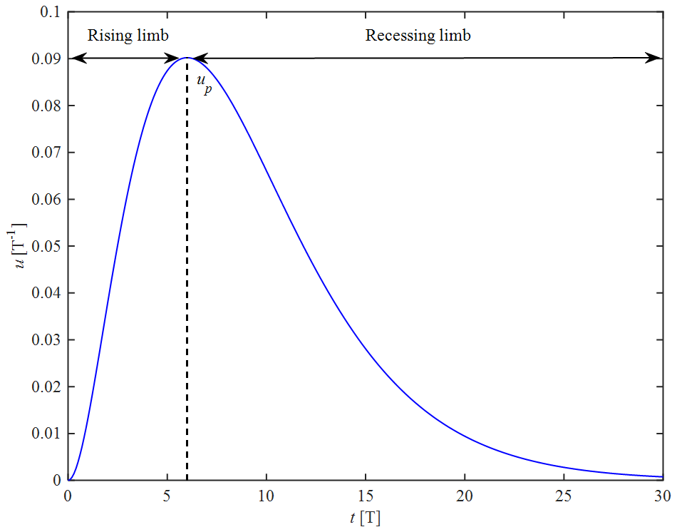
Figure 1Illustration of the instantaneous UH analytically computed using Eq. (6) for given values of .
Although Eq. (6) is widely used as the analytical solution of an instantaneous UH, it has the following two weaknesses: (1) it has an initial condition of zero, which is not necessarily the case for real instantaneous UHs; and (2) a general and analytical solution of the S-hydrograph does not exist. In order to remove these weaknesses, Guo (2022a) made the following three hypotheses on the instantaneous UH based on empirical observations: (1) the instantaneous UH increases exponentially along the rising limb; (2) the instantaneous UH decreases exponentially along the recessing limb; (3) the instantaneous UH tends towards 0, and the S-hydrograph tends towards 1, as t tends towards infinity. Subsequently, he derived the following general and analytical solution for the S-hydrograph:
where β1 is the dimensionless rising coefficient determined by the watershed characteristics, β2 is the dimensionless recessing coefficient affected by the downstream water surface condition, while t=tp corresponds to the inflection point with the maximum instantaneous UH as follows:
With Eq. (7), the instantaneous UH u(t) is expressed as
To illustrate the general and analytical solutions of the S-hydrograph from Eq. (7) and of the instantaneous UH from Eq. (9), Fig. 2 shows the computed U(t) (solid line) and u(t) (dashed line) for given values of 3 and tp=10.

Figure 2Illustration of the S-hydrograph and instantaneous UH analytically computed using Eqs. (7) and (9), respectively, for given values of and tp=10.
2.2 Savenije's salt intrusion model
In estuaries, the key to deriving an empirical relationship for the salinity distribution is the dispersion coefficient, which is either constant (e.g., Gay and O'Donnell, 2007) or variable (e.g., Van der Burgh, 1972; Prandle, 1981). Based on the effective tidal average dispersion under steady-state conditions, Van der Burgh (1972) proposed the following empirical relationship for the dispersion coefficient:
where D [L2T−1] is the longitudinal dispersion coefficient, x [L] is the longitudinal coordinate measured in the upstream direction, Q [L3T−1] is the fresh-water discharge, A [L2] is the tidally averaged cross-sectional area, and K is the dimensionless Van der Burgh coefficient.
It is assumed that the longitudinal cross-sectional area follows an exponential function as follows:
where A0 is the cross-sectional area at the estuary mouth, and a is the convergence length. Integration of Eq. (10) and taking into account the exponential variation of the cross-sectional area using Eq. (11) yields the following analytical description of the longitudinal effective dispersion (Savenije, 2005, 2012):
where D0 is the dispersion coefficient at the estuary mouth.
With Eq. (10), Savenije (2005, 2012) derived a one-dimensional empirical model for salt intrusion based on the tidally averaged cross-sectional mass conservation equation:
where F [MT−1] and S [ML−3] are the tidally averaged salt flux and salinity, respectively.
In a steady-state situation with no net salt flux (i.e., F=0), Eq. (13) can be rewritten as follows:
We can combine Eqs. (10) and (14) into a general relationship between the dispersion coefficient and salinity through the Van der Burgh's coefficient as follows (Savenije, 2005, 2012):
where S0 is the salinity concentration at the estuary mouth.
Combing Eqs. (12) and (15) yields the tidally averaged salinity along an estuary as follows (Savenije, 2005, 2012):
To make Eq. (16) dimensionless, we introduce the following dimensionless parameters:
where S∗ is the dimensionless salinity that is scaled by the value at the estuary mouth, γ represents the estuary shape number describing the convergence rate of an estuary, ω is the tidal frequency, D∗ is the dimensionless dispersion coefficient representing the downstream dispersion condition, x∗ is the dimensionless longitudinal coordinate that is normalized by the frictionless wavelength in prismatic channels, and c0 is the classical wave celerity of a frictionless progressive wave, which is defined as
in which g [LT−2] is the acceleration due to gravity, h [L] is the tidally averaged depth, and rS is the storage width ratio (see Savenije et al., 2008). Here, the asterisk denotes a dimensionless variable.
Thus, Eq. (16) can be rearranged as follows (Cai et al., 2015):
With Eq. (19), it is possible to derive an analytical expression for the salt intrusion length (i.e., the distance from the estuary mouth to the location where the water is totally fresh), which is obtained by setting in Eq. (19) as follows:
Suppose there is an ocean coupling to an estuary with the coordinate origin located at the estuary mouth. If a unit volume of excess salinity from the ocean is locally (Δx→0) released into the estuary during the time required for an equilibrium to occur, the resulting hydrograph is the instantaneous UH that corresponds to the S-hydrograph S∗(x) in the dimensionless form. Similar to Guo's UH method (Guo, 2022a), we make four hypotheses on the instantaneous UH (representing the instantaneous rate of change with respect to the salinity at a specific position along the estuary axis, i.e., the salinity gradient) for the salinity distribution based on depth-average observations along estuaries (i.e., data facts).
-
Hypothesis 1. Along the recessing limb, the salinity gradient decreases exponentially, which makes the salinity S∗(x) decay exponentially in a convex shape.
-
Hypothesis 2. The salinity is scaled by the almost-constant salinity in the deep ocean, i.e., approximately 36 kg m−3; thus, as x tends towards negative infinity, the salinity gradient tends towards zero, and the salinity S∗(x) tends towards 1.
-
Hypothesis 3. Along the rising limb, the salinity gradient increases exponentially, which makes the salinity S∗(x) decay exponentially in a concave shape.
-
Hypothesis 4. As x tends towards infinity, the salinity gradient tends towards zero, and the salinity S∗(x) tends towards zero.
It should be noted that the above hypotheses 1 and 3 are, in principle, valid only for well-mixed or partially mixed estuaries, where salt intrusion really matters. From a practical perspective, this is not a restrictive assumption, since the salt wedge in highly stratified conditions only occurs at the time of high river discharge, when flood protection is generally the main concern and salt intrusion is not relevant (Savenije, 2005, 2012).
According to the first hypothesis, along the recessing limb, and S∗(x) satisfy the following relationship:
where μ represents the recessing coefficient [L−1]. Meanwhile, the second hypothesis requires that and that 1 (representing the constant salinity in the ocean) at . To meet this requirement, we revise Eq. (21) as follows:
since . Integrating Eq. (22) for S∗(x) and applying the initial condition (i.e., x=0, results in
Similarly, according to the third hypothesis, along the rising limb, we have
where m represents the dimensionless rising coefficient. Integrating Eq. (24) for S∗(x) and applying the initial condition (i.e., x=0, results in
which satisfies the fourth hypothesis. We can combine Eqs. (22) and (24) into a generalized differential equation as follows:
which reduces to Eq. (22) at where and Eq. (24) at x→∞ where . The inflection point x=xp, where
corresponds to the maximum absolute value of (i.e., the maximum salinity gradient). Integrating Eq. (26) for S∗(x) and applying Eq. (27) results in
To make μ dimensionless, we make a transform, namely μxp→μ; then Eq. (28) can be revised as:
where /xp is the dimensionless distance scaled by the position of the inflection point xp. With Eq. (29), the instantaneous UH is written as
which satisfies the general UH definition; i.e., .
It can be seen from Eq. (28) that the theoretical salt intrusion length L∗ is not available, since S∗ tends towards 0 as x approaches infinity asymptotically. However, it is possible to define a specific salt intrusion length for a given salinity threshold (such as 0.01) by substituting into Eq. (29) as follows:
Figure 3 illustrates the spatial distribution of the S-hydrograph (salinity distribution S∗) and its instantaneous UH (salinity gradient for given values of μ=1.5 and m=1.
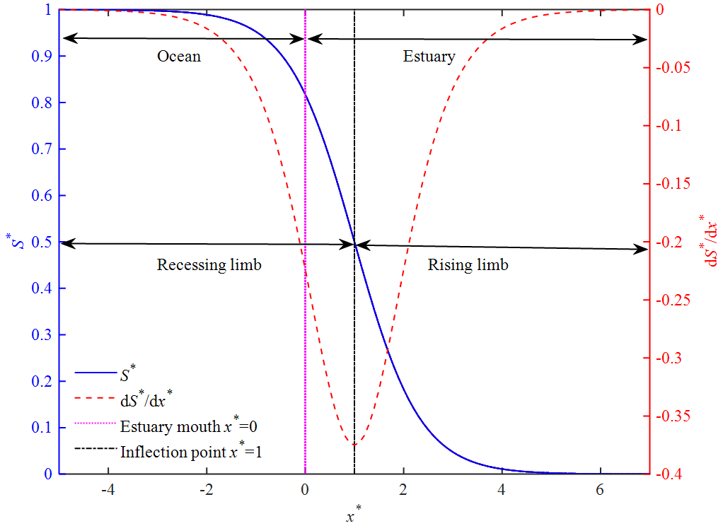
Figure 3S-hydrograph S∗ (salinity concentration) and its instantaneous UH (salinity gradient) as a function of the dimensionless along-estuary distance x∗ for given values of μ=1.5, m=1.
4.1 Sensitivity analysis of the proposed salt intrusion model
Although Eqs. (29), (30) and (31) are analytical, the sensitivity to the two controlled parameters (μ and m) is not straightforward and directly clear. Thus, it is worthwhile to have a sensitivity analysis on the two calibrated parameters. Figure 4 presents the analytical solutions of the longitudinal salinity and its gradient as a function of μ and m. It can be clearly seen from Fig. 4 that two distinct estuarine regions display a very different behavior. For , we see an exponential decrease of the salinity gradient until a minimum value is reached at a critical position x=xp (or ) defined by Eq. (27), beyond which the salinity gradient increases exponentially until zero is reached asymptotically (Fig. 4c, d). The sensitivity analysis shows that the recessing coefficient μ determines the change rate of both the rising and recessing limbs (Fig. 4a, c). With regard to the rising coefficient m, it can be seen from Fig. 4b that the coefficient m exerts more influence along the rising limb and thus affects mainly the salinity distribution after the inflection point (Fig. 4b, d). In addition, Fig. 4c and d show that m=1 gives a symmetric salinity gradient of about x=xp (, ), gives a negatively skewed salinity gradient, and m>1 gives a positively skewed salinity gradient.
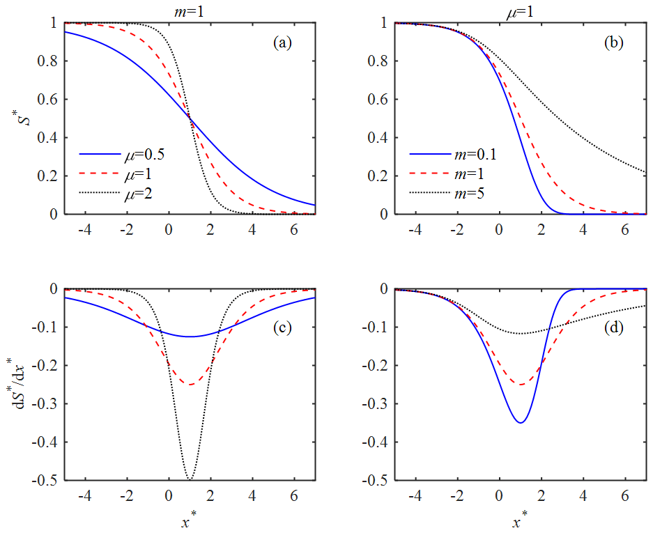
Figure 4Sensitivity analysis of the dimensionless salinity S∗ and its gradient with regard to the recessing coefficient μ and the rising coefficient m.
To understand the response of the salt intrusion length to both calibrated parameters, Eq. (31) was used to analytically compute L∗ for a wide range of μ and m values (Fig. 5) considering a salinity threshold of . We can clearly see that the isolines are almost linear, converging towards the origin of the m–μ diagram. Generally, the salt intrusion length increases with m, while it decreases with μ. This suggests that the model parameter m is generally proportional to the strength of tidal dynamics that induce dispersive transport of salt in the upstream direction, while the model parameter μ is proportional to the strength of the riverine flushing seaward. With this plot, it is possible to understand the potential impacts of different hydrodynamic conditions on the salt intrusion length, which is particularly useful to decision makers for salt intrusion prevention.
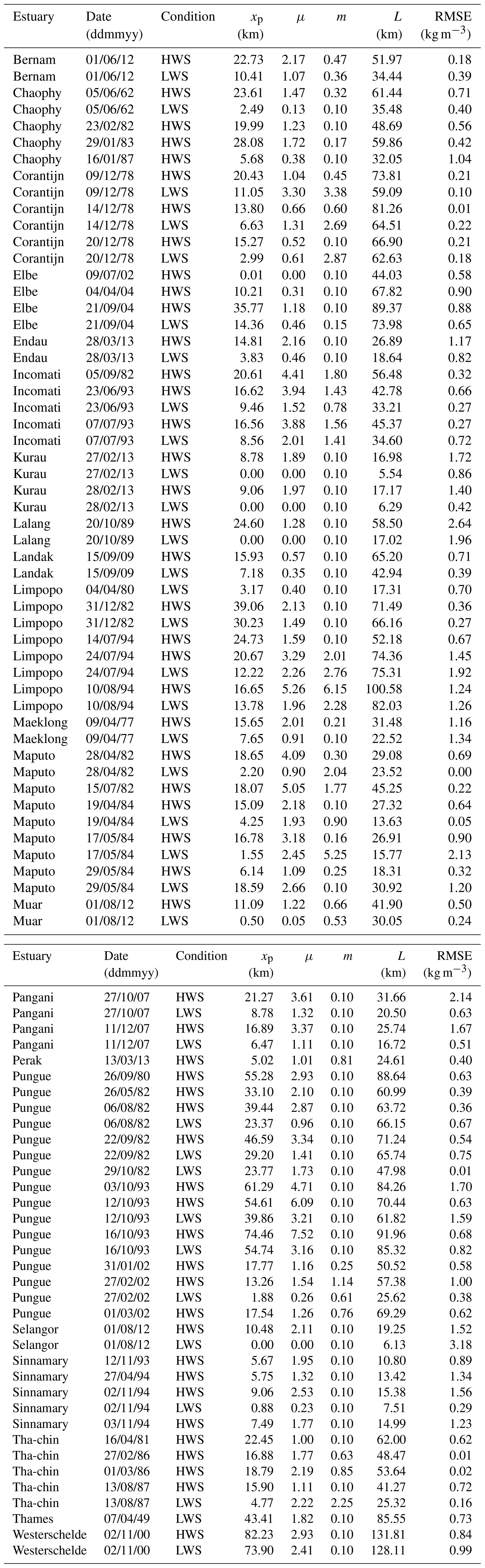
Table 1Measured salinity distribution, calibrated parameters, computed salt intrusion length and model performance in terms of RMSE.
4.2 Application to real estuaries
The proposed salt intrusion model has been applied to observations in real estuaries worldwide with a wide range of different riverine and tidal hydrodynamics. In Table 1, a selection is presented for 21 estuaries where 89 salt intrusion measurements were collected at either high water slack (HWS) or low water slack (LWS; all observations are available on the web at https://salinityandtides.com/data-sources/, last access: 3 May 2023). In this table, the three model parameters xp, μ and m were obtained by fitting Eq. (29) to the observed longitudinal salt intrusion. This can be easily done by means of a nonlinear curve-fitting method in the least-squares sense (such as using the MATLAB “lsqcurvefit.m” function). The model performance was evaluated by using the root-mean-square error (RMSE). Figure 6 shows the comparison of the observed and computed salinity concentrations in different estuaries. It can be seen from Fig. 6 that the correspondence with the observed salt intrusion is good, with the RMSE being 1.1 kg m−3 on average (see also the model performance reported in Table 1 for many estuaries worldwide with distinct salt intrusion lengths).
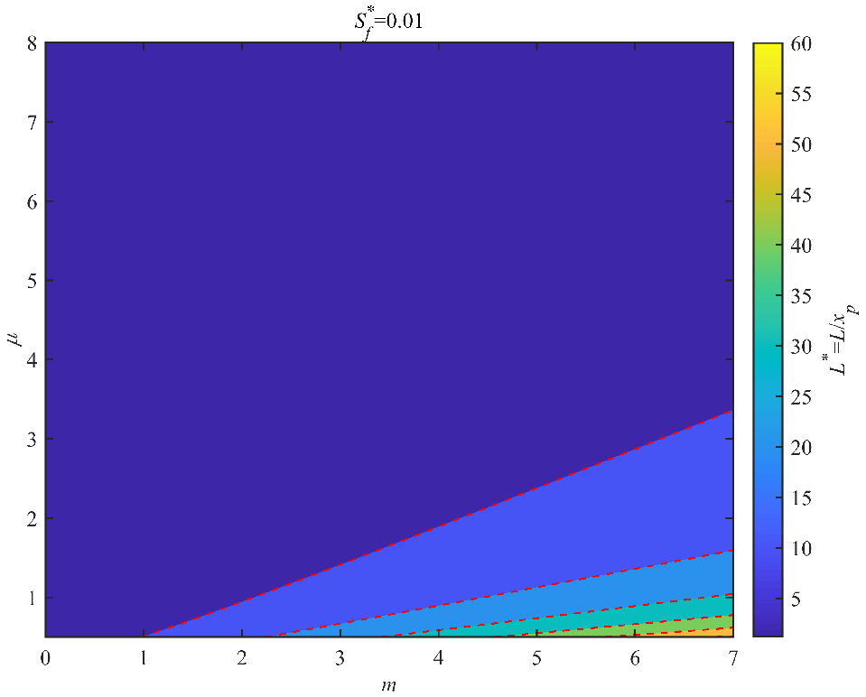
Figure 5Response of the salt intrusion length L∗ to the dimensionless parameters μ and m for a given salinity threshold .
For illustrations, Fig. 7 shows the longitudinal computation applied to the Pungue, Incomati and Limpopo estuaries by means of both the newly proposed and Savenije's models. Generally, the results of the two models are satisfactory for the following different shapes of salt intrusion curves in well-mixed or partially mixed estuaries (Savenije, 2005, 2012): (1) a dome-shape intrusion curve (such as along the Pungue estuary – Fig. 7a), which generally occurs in strong funnel-shaped estuaries; (2) a bell-shaped intrusion curve (such as along the Incomati estuary – Fig. 7c), which generally occurs in estuaries that have a trumpet shape; (3) a recession-shape intrusion curve (such as along the Limpopo estuary – Fig. 7e), which generally occurs in narrow estuaries with a near-prismatic shape and a high river discharge. It is worth noting that these types of salt intrusion curves are very much linked to the geometry of the estuary (Savenije, 2005, 2012). However, we observe from Table 1 that the calibrated model parameters (μ and m) are rather sensitive to the varied riverine and tidal forcing for a specific estuary. Thus, further studies concerning the relationship between the forcing conditions and the model parameters (μ and m) are required in the future. It can be seen from Fig. 7 that one important difference in terms of performance between these two models lies in the rising limb when the distance approaches infinity. As x tends towards infinity, the salinity gradient of the newly proposed model asymptotically approaches zero, while it reduces to zero at a critical position corresponding to the salt intrusion length from Eq. (20) for Savenije's model. This feature allows an improved fit with observations at the toe of the salt intrusion curve (e.g., Fig. 7a). Figures S1–S8 in the Supplement show the comparison between the observed longitudinal salinity and the analytically computed salt intrusion curves along 21 estuaries worldwide (see the Supplement).
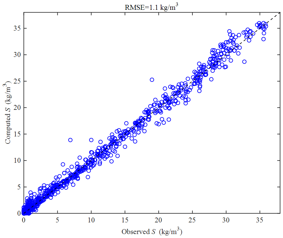
Figure 6Comparison between the analytically computed salinity concentrations and 89 observations in 21 estuaries worldwide.
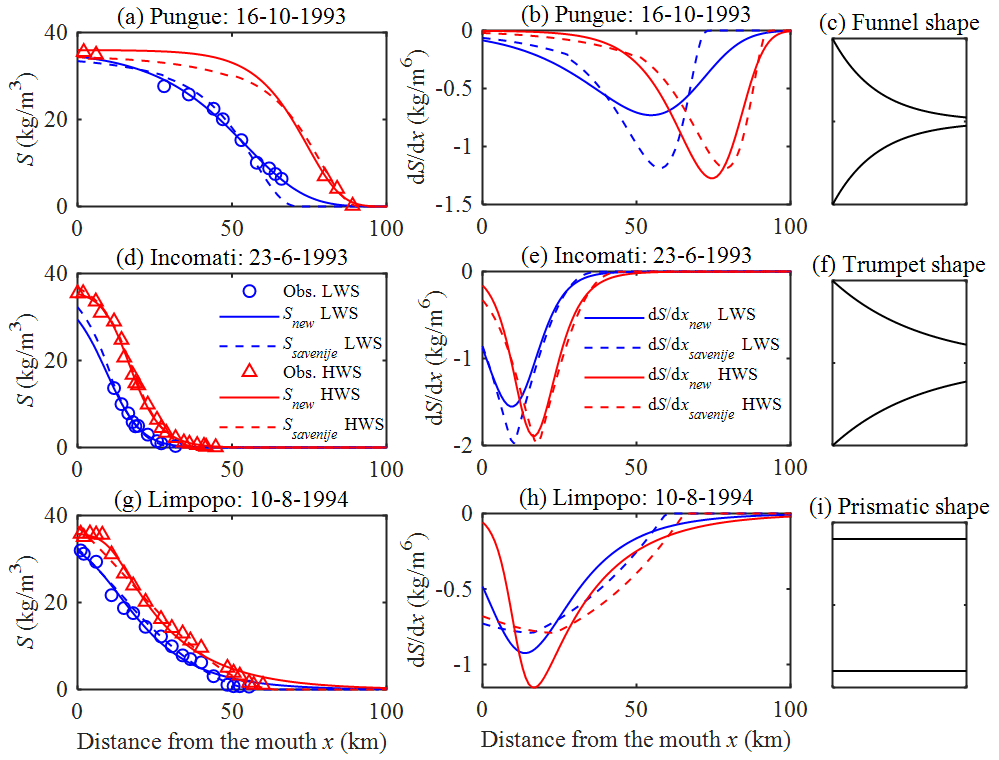
Figure 7Observed and analytically computed salt intrusion curves using the newly proposed and Savenije's models in the Pungue estuary (a, b), in the Incomati estuary (d, e) and in the Limpopo estuary (g, h), together with the idealized shape of the estuary ((c) funnel shape, (f) trumpet shape and (i) prismatic shape).
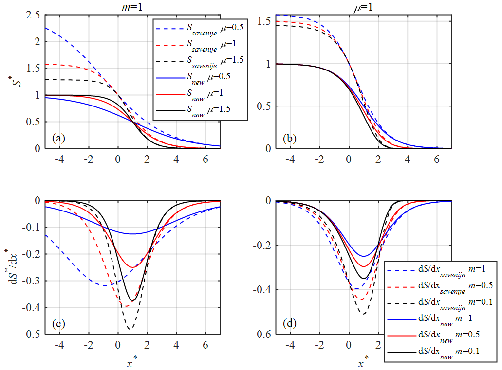
Figure 8Longitudinal variations of the dimensionless salinity S∗ (a, b) and its gradient (c, d) along the estuary axis for different values of input parameters. The solid and dashed lines indicate the solutions obtained by Savenije's model and the newly proposed model, respectively.
4.3 Analytical difference with Savenije's salt intrusion model
In order to understand the differences between the newly proposed model and empirical solutions based on the steady salt balance equation, we have made a comparison with the widely used Savenije's salt intrusion model (Savenije, 2005, 2012) by means of a Taylor expansion. The Taylor expansion of Savenije's salt intrusion model, i.e., Eq. (19), is written as
To make a comparison of the proposed model (i.e., Eq. 29) with Eq. (19), we introduce (Van der Burgh's coefficient); then Eq. (29) becomes
The Taylor expansion of Eq. (33) is written as
It is difficult to directly compare Eqs. (32) and (34). Alternatively, the difference between Eqs. (19) and (33) can be explored by looking at the exponential function parts, which can be expanded by the Taylor series as follows:
Interestingly, if we slightly modified Eq. (35) by removing 1 from the brackets, then the Taylor expansion of Eq. (35) can be rewritten as
In this case, Eqs. (36) and (37) are identical if they satisfy the following conditions:
Thus, for given prior conditions Eqs. (38) and (39), the main difference between the newly proposed model and Savenije's model lies in the inclusion of the term – in the braces of Eq. (33), which is closely related to the upstream river discharge, the dispersion coefficient at the estuary mouth, the tidal frequency and the geometry of the estuary according to Eq. (17). As an illustration, Fig. 8 displays the longitudinal variations of the dimensionless salinity S∗ and its gradient for different values of the recessing coefficient μ and the rising coefficient m, where the solid and dashed lines represent the solutions obtained by Savenije's model and the newly proposed model, respectively. It can be seen from Fig. 8 that the additional term mexp (−μ) mainly affects the downstream part of the salt intrusion curve, while the two methods tend to be the same for larger values of x∗ (at the toe of the salt intrusion curve).
It is worth noting that the above analysis suggests that Van der Burgh's coefficient K (being equal to −m) should be negative rather than positive, since m is generally positive (see Table 1). This indicates that the dispersion coefficient D should be increased along the estuary axis according to Eq. (10). Figure 9 shows the analytically computed longitudinal dimensionless salinity S∗ using Eq. (19) for a wide range of the input parameters K and D∗ when γ=1. We can see that the computed S∗ does converge to 0 when the distance x∗ approaches infinity when K values are negative, which is very different from the performance of the previous analytical solutions using positive K values, where the computed S∗ generally diverges for larger values of x∗. Consequently, from a curve-fitting perspective, the Savenije's model using negative K values can be regarded as a special case of the newly proposed salt intrusion model if we further rescale the salinity by the dimensionless salinity in the deep ocean (see Fig. S9 in the Supplement). This also suggests that an enhanced empirical relationship concerning the effective dispersion coefficient (instead of the conventional Van der Burgh's relationship) is required for deriving an accurate salt intrusion curve from a theoretic point of view.
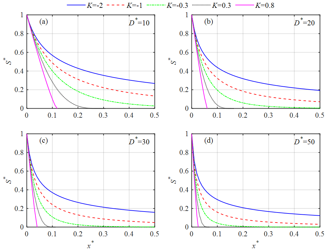
Figure 9Longitudinal variation of the dimensionless salinity S∗ computed using Eq. (19) along the estuary axis for different values of K and D∗ when γ=1.
It should be noted that, although the model fits the observations very well, the physical foundation of Eq. (29) needs further study in the future. This limitation could be relaxed by carefully comparing the proposed model with those based on the steady-state salt balance equation. Specifically, several idealized numerical models (1-D, 2-D or 3-D models) have been adopted as a first approximation to quantify the along-channel salinity dynamics (e.g., Pein et al., 2018; Dijkstra and Schuttelaars, 2021; Wei et al., 2022). With these idealized numerical models, the physics behind Eq. (29) can be understood in order to make the model fully predictive through the relation of the three model parameters (xp, μ and m) to measurable or quantifiable variables (e.g., river discharge, tidal amplitude and cross-sectional area convergence length) by means of regression techniques or similar approaches. It should be noted that the proposed salt intrusion model is, in principle, valid only for well-mixed or partially mixed estuaries, where salt intrusion really matters. From a practical perspective, this is not a restrictive assumption, since the salt wedge in highly stratified conditions only occurs at the time of high river discharge, when flood protection is generally the main concern and salt intrusion is not relevant (Savenije, 2005, 2012). Moreover, the proposed salt intrusion model is particularly useful for quantifying the alterations in salt intrusion dynamics owing to climate change or human interventions by comparing the three calibrated model parameters for different periods with considerably different conditions.
In this paper, we revisited the empirical salt intrusion model, making use of Guo's general unit hydrograph theory (Guo, 2022a, b, c), and proposed a general and analytical model for the salinity distribution in estuaries of the partially mixed to well-mixed types. The newly developed method does not require observed or calibrated salinity at the estuary mouth and can be well calibrated using a minimum of three salt measurements along the estuary axis. This is mainly due to the fact that Eq. (29) is a monotonic function whose first derivative (i.e., Eq. 30) does not change sign and has only one minimum. In addition, the salinity converges towards zero as the along-estuary distance approaches infinity asymptotically, which might improve the model performance near the toe of the salt intrusion curve when compared to empirical solutions based on the salt balance equation. The model has been applied to numerous estuaries worldwide, and the results agree very well with the observations. This indicates that the proposed model can be a useful tool to understand the dynamics of salt intrusion in estuaries and for assessing the potential impacts of human-induced (e.g., dredging) or natural (e.g., mean sea level rise) changes. However, the underlying physical foundation of the proposed model and the physics of the model parameters need further study in the future.
All salt intrusion observations are available on the website at https://salinityandtides.com/data-sources/ (Savenije, 2023).
The supplement related to this article is available online at: https://doi.org/10.5194/os-19-603-2023-supplement.
All the authors contributed to the design and development of this work. The model was originally developed by HC. BL and JG carried out the data analysis. EG revised the paper. TZ reviewed the paper.
The contact author has declared that none of the authors has any competing interests.
Publisher’s note: Copernicus Publications remains neutral with regard to jurisdictional claims in published maps and institutional affiliations.
The first author very much appreciates the valuable suggestions from Guo Junke of University of Nebraska Lincoln in the derivations of Eqs. (20)–(30). The very valuable comments from Hubert Savenije of TU-Delft are very much appreciated.
This research has been supported by the National Natural Science Foundation of China (grant no. 51979296, 52279080), from the Guangdong Provincial Department of Science and Technology (grant no. 2019ZT08G090), and from the Guangdong Provincial Bureau of Hydrology (grant no. 440001-2023-10716). EG received support from FCT through the grants LA/P/0069/2020 awarded to the Associate Laboratory ARNET and UID/00350/2020 awarded to CIMA, University of Algarve.
This paper was edited by Jochen Wollschlaeger and reviewed by Daniel Thewes and one anonymous referee.
Cai, H., Savenije, H. H. G., Zuo, S., Jiang, C., and Chua, V.: A predictive model for salt intrusion in estuaries applied to the Yangtze estuary, J. Hydrol., 529, 1336–1349, https://doi.org/10.1016/j.jhydrol.2015.08.050, 2015.
Chow, V. T., Maidment, D., and Mays, L. W.: Applied hydrology, New York, McGraw-Hill, ISBN 0-07-100174-3, 1988.
Dijkstra, Y. M. and Schuttelaars, H. M.: A unifying approach to subtidal salt intrusion modeling in tidal estuaries, J. Phys. Oceanogr., 51, 147–167, https://doi.org/10.1175/jpo-d-20-0006.1, 2021.
Gay, P. and O'Donnell, J.: Comparison of the salinity structure of the Chesapeake Bay, the Delaware Bay and Long Island Sound using a linearly tapered advection-dispersion model, Estuar. Coast., 32, 68–87, https://doi.org/10.1007/s12237-008-9101-4, 2009.
Gay, P. S. and O'Donnell, J.: A simple advection-dispersion model for the salt distribution in linearly tapered estuaries, J. Geophys. Res.-Oceans, 112, C070201, https://doi.org/10.1029/2006JC003840, 2007.
Guo, J.: General and analytic unit hydrograph and its applications, J. Hydrol. Eng., 27, 04021046, https://doi.org/10.1061/(ASCE)HE.1943-5584.0002149, 2022a.
Guo, J.: General unit hydrograph from Chow's linear theory of hydrologic systems and its applications, J. Hydrol. Eng., 27, 04022020, https://doi.org/10.1061/(ASCE)HE.1943-5584.0002184, 2022b.
Guo, J.: Application of general unit hydrograph model for baseflow separation from rainfall and streamflow data, J. Hydrol. Eng., 27, 04022027, https://doi.org/10.1061/(ASCE)HE.1943-5584.0002217, 2022c.
Kuijper, K. and Van Rijn, L. C.: Analytical and numerical analysis of tides and salinities in estuaries; part II: salinity distributions in prismatic and convergent tidal channels, Ocean Dynam., 61, 1743–1765, https://doi.org/10.1007/s10236-011-0454-z, 2011.
Lewis, R. E. and Uncles, R. J.: Factors affecting longitudinal dispersion in estuaries of different scale, Ocean Dynam., 53, 197–207, https://doi.org/10.1007/s10236-003-0030-2, 2003.
Nash, J. E.: The form of instantaneous unit hydrograph, Int. Assoc. Sci. Hydrol. Publ., 45, 114–121, 1957.
Pein, J., Valle-Levinson, A., and Stanev, E. V.: Secondary circulation asymmetry in a meandering, partially stratified estuary, J. Geophys. Res.-Oceans, 123, 1670–1683, https://doi.org/10.1002/2016JC012623, 2018.
Prandle, D.: Salinity intrusion in estuaries, J. Phys. Oceanogr., 11, 1311–1324, https://doi.org/10.1175/1520-0485(1981)011<1311:SIIE>2.0.CO;2, 1981.
Savenije, H. H. G.: A one-dimensional model for salinity intrusion in alluvial estuaries, J. Hydrol., 85, 87–109, https://doi.org/10.1016/0022-1694(86)90078-8, 1986.
Savenije, H. H. G.: Salt intrusion model for high-water slack, low-water slack, and mean tide on spread sheet, J. Hydrol., 107, 9–18, https://doi.org/10.1016/0022-1694(89)90046-2, 1989.
Savenije, H. H. G.: Predictive model for salt intrusion in estuaries, J. Hydrol., 148, 203–218, https://doi.org/10.1016/0022-1694(89)90046-2, 1993.
Savenije, H. H. G.: Salinity and tides in alluvial estuaries, New York, Elsevier, https://doi.org/10.1016/B978-0-444-52107-1.X5000-X, 2005.
Savenije, H. H. G.: Salinity and tides in alluvial estuaries, completely revised 2nd edition, http://www.salinityandtides.com (last access: 22 March 2022), 2012.
Savenije, J. H.: Data_SalinityandTides, WordPress [data set], https://salinityandtides.com/data-sources/ (last access: 3 May 2023), 2012.
Van der Burgh, P.: Ontwikkeling van een methode voor het voorspellen van zoutverdelingen in estuaria, kanalen en zeeen, Den Haag, Rijkwaterstaat Rapport, 10–72, 1972 (in Dutch).
Wei, X., Williams, M. E., Brown, J. M., Thorne, P. D., and Amoudry, L. O.: Salt intrusion as a function of estuary length in periodically weakly stratified estuaries, Geophys. Res. Lett., 49, e2022GL099082, https://doi.org/10.1029/2022GL099082, 2022.
Zhang, Z. and Savenije, H. H. G.: The physics behind Van der Burgh's empirical equation, providing a new predictive equation for salinity intrusion in estuaries, Hydrol. Earth Syst. Sci., 21, 3287–3305, https://doi.org/10.5194/hess-21-3287-2017, 2017.
Zhang, Z. and Savenije, H. H. G.: Thermodynamics of saline and fresh water mixing in estuaries, Earth Syst. Dynam., 9, 241–247, https://doi.org/10.5194/esd-9-241-2018, 2018.
- Abstract
- Introduction
- Review of the general unit hydrograph and empirical salt intrusion model
- General unit hydrograph theory for salt intrusion
- Results and discussion
- Conclusions
- Data availability
- Author contributions
- Competing interests
- Disclaimer
- Acknowledgements
- Financial support
- Review statement
- References
- Supplement