the Creative Commons Attribution 4.0 License.
the Creative Commons Attribution 4.0 License.
 | 19 Jul 2023
Variability in coastal downwelling circulation in response to high-resolution regional atmospheric forcing off the Pearl River estuary
Wenfeng Lai
Jianping Gan
We investigated the variabilities in coastal circulation and dynamics in response to spatiotemporally variable high-resolution atmospheric forcing off the Pearl River estuary during the downwelling wind. Our investigation focused on the dynamics of coastal downwelling circulation in response to variable atmospheric forcing of (1) single-station observation, (2) global reanalysis data, and (3) a high-resolution regional atmospheric model. We found that the high-resolution atmospheric model significantly improved the representations of the near-surface wind and air temperature, and the ocean model driven by the high-resolution and spatially variable atmospheric forcing improved the circulation and associated hydrographic properties in the coastal ocean. Momentum and vorticity analyses further revealed that the cross-isobath water exchange was primarily governed by the along-isobath pressure gradient force (PGF), which was influenced by different components of the atmospheric forcing. The spatial–temporal variability in high-resolution wind forcing determined the strength and structure of coastal circulation and improved estimates of cross-isobath transport and the associated PGF by refining the net stress curl and nonlinear advection of relative vorticity in the simulation. The high-resolution heat forcing can greatly improve the sea surface temperature simulation and adjust the nonlinear advection of relative vorticity, resulting in changes in cross-isobath transport.
- Article
(17929 KB) - Full-text XML
- BibTeX
- EndNote


Accurate representations of momentum and heat fluxes are essential for accurate ocean modeling, especially for complex coastal zones where the forcing is highly influenced by land–sea interactions. In numerical ocean simulations, atmospheric forcing is generally obtained from an observation station within the study area (Zu and Gan, 2015), large-scale reanalysis data (Liu and Gan, 2020), or idealized wind assumptions (Xie and Eggleston, 1999). However, these common methods neither reflect nor resolve the complex regional variations in atmospheric fluxes in the coastal zone that result from local topographic features and land–air–sea interactions. Several factors, such as the representation of topography, land–atmospheric interactions, surface heat and moisture fluxes, and physical processes parameterizations, can influence the accuracy of meteorological variable simulation, such as that of near-surface winds and air temperature (e.g., Cheng and Steenburgh, 2005; Singh et al., 2021). Inaccurate representation of wind fields can lead to incorrect ocean current structures and significant biases in sea surface temperature (SST). Numerical ocean simulation can benefit from higher-resolution atmospheric forcing, which can help resolve, for example, oceanic mesoscale processes in ocean circulation (Jung et al., 2014).
Here we explore the important factors which can influence the response of coastal ocean circulation and associated dynamics to high-resolution atmospheric forcing in the Pearl River estuary (PRE). We conduct comparative analyses of the simulated results forced with different resolutions of atmospheric fluxes. The PRE has a “trumpet” shape, with a width of 5 km at the northern end and 35 km at the southern end. Two longitudinally deep channels in the central and eastern regions connect the PRE to the adjacent shelf in the northern South China Sea (NSCS) where isobaths are approximately parallel to the coastline, forming a strong cross-shelf topographic gradient. Local and highly spatially variable winds and strong land–sea breezes have significant impacts on circulation patterns in the estuary–shelf area around the PRE (Lai et al., 2021). Down-estuary winds can intensify the stratification of the water column and can also strengthen the along-estuary exchange circulation through wind-induced straining. In contrast, an up-estuary wind will enhance vertical mixing and weaken the estuarine circulation (Lai et al., 2018). During the summer/winter, the freshwater plume extends eastward/westward over the shelf, where it interacts with the monsoon-driven currents (Pan et al., 2020). Seaward gravitational convection characterizes the circulation within the PRE, while the circulation in the lower estuary is governed by a combination of gravitational convection and intrusive geostrophic currents from the shelf (Zu et al., 2014). Throughout the NSCS, coastal downwelling and upwelling circulations are strongly influenced by the alongshore wind stress and wind stress curl (Gan et al., 2015; Lai and Gan, 2022). The coastal circulation and water properties in and near the PRE are sensitive to highly variable atmospheric forcing, such as wind and heat flux.
Higher-resolution regional atmosphere models can better reproduce the variability in atmospheric momentum and heat fluxes by resolving complex terrain and result in improved forecast skills (Agustsson and Olafsson, 2007). Akhtar et al. (2017) found that using a 9 km resolution atmosphere model resulted in improved simulations of wind speed and turbulent heat flux compared to using a 50 km resolution model. High-resolution regional atmospheric models provide significant new insights by parameterizing or explicitly simulating atmospheric processes over finer spatial scales. As an example, extreme atmospheric events in the Mediterranean coastal region can be better simulated by resolving fine details of land use and topography and explicit convection simulations (Hohenegger et al., 2008).
Numerical modeling of estuarine and coastal systems is often limited by the quality of atmospheric forcing data used (Myksvoll et al., 2011). Upper-ocean currents and turbulent mixing are sensitive to small-scale variations in atmospheric forcing. According to Pullen et al. (2003), ocean current predictions were more accurate and skillful when using a 4 km resolution atmospheric forcing compared with a 36 km spacing. Similarly, high-resolution atmospheric forcing allowed for more realistic reproduction of circulation in the Gulf of Lions due to better representations of the oceanic mixed-layer characteristics and dynamics in the ocean model (Langlais et al., 2009). Kourafalou and Tsiaras (2007) found that high-resolution atmospheric forcing allowed for a rapid oceanic response to large-scale wind variability in the northern Aegean Sea, resulting in reasonable changes in water properties and circulation. The precise wind stress and wind stress curl structures near the coast from high-resolution forcing improved simulations of coastal jet in eastern boundary upwelling systems, leading to a significant reduction in warm biases in SST (Small et al., 2015). Finally, the capabilities to describe thermohaline circulation and water mass formation processes were improved under increased spatiotemporal resolution of atmospheric forcing at a regional scale (Castellari et al., 2000; Artale et al., 2016).
Accurate representation of atmospheric forcing is critical to correctly simulating the spatiotemporal variability in coastal circulation and biogeochemical processes in coupled estuary–shelf systems. To thoroughly study the variability in the coastal ocean circulation, a combination of a state-of-the-art ocean model and high-resolution atmospheric forcing is required. In a recent study, Lai and Gan (2022) compared the impacts of low-resolution global reanalysis data and high-resolution wind forcing on the coastal circulation during upwelling-favorable winds and found that a high-resolution regional atmosphere model tended to produce stronger surface wind stresses, resulting in an intensified cross-isobath transport off the PRE. However, despite this region being primarily dominated by the prevailing southwesterly monsoon (upwelling-favorable wind) during summer, the PRE also experiences episodic downwelling-favorable wind, which can significantly alter the pathway of river plume, coastal circulation, and cross-shore water transport. The alternations of the downwelling circulation under the spatiotemporally variable atmospheric fluxes and plume-induced buoyancy demonstrated the important wind-driven circulation dynamics.
In this study, our objective is to systematically investigate the responses of small-scale coastal circulation and associated dynamics to different resolution atmospheric forcings off the PRE during the downwelling-favorable wind. We aim to isolate the impacts of uniform wind, low-resolution wind, high-resolution wind, and heat flux forcing on the coastal downwelling circulation. To achieve this, we perform dynamics analyses on the coastal wind-driven ocean circulation under forcing of momentum and heat fluxes using the following: (1) local station observations, (2) global reanalysis data, and (3) a high-resolution regional atmospheric model. An improved understanding of the responses of oceanic processes and underlying dynamics to spatiotemporal variability in atmospheric forcing will advance our physical and numerical understanding and enhance the accuracy of coastal ocean modeling.
We ran a high-resolution regional atmospheric model to dynamically downscale large-scale reanalysis data and to obtain fine atmospheric forcing for our coastal ocean model in the PRE. The surface heat budget and near-surface wind field derived from the model variables were used as surface boundary conditions for the ocean model.
2.1 The regional atmospheric model
We used the Weather Research and Forecasting (WRF) model to simulate the regional atmospheric environment in the PRE and NSCS. The WRF is a mesoscale, non-hydrostatic, numerical weather prediction model with advanced physics and numerical schemes for simulating meteorology and dynamics (Michalakes et al., 1999). This model adopts a fully compressible, non-hydrostatic model with a horizontal Arakawa C grid and terrain-following coordinates in the vertical direction.
A dynamical downscaling technique was employed in the WRF model to obtain a higher-resolution output (Caldwell et al., 2009) and better resolve the influence of regional dynamics and topography. A three-domain-nested configuration was designed, as depicted in Fig. 1a. The outer domain (D01) covered the western Pacific Ocean, the entire South China and East China seas, and the Sea of Japan and had a horizontal resolution of 9 km. The middle domain (D02) covered the NSCS with a horizontal resolution of 3 km. The inner domain (D03) had a high-resolution spacing of 1 km and covered the Guangdong–Hong Kong–Macau Greater Bay Area. The US Geological Survey provided static geographical data, including land use and topographical information, with a horizontal resolution of 30 arcsec (approximately 0.9 km). All domains had 33σ layers in the vertical direction, and the maximum top-layer pressure was 50 hPa. The initial conditions and lateral boundary conditions for the outer domain were provided by the reanalyses (ERA-Interim) data from the European Centre for Medium-Range Weather Forecasts (ECMWF). The physics options of the WRF model included the WSM6 microphysics scheme (Hong et al., 2006a), CAM shortwave and longwave radiation schemes (Collins et al., 2004), YSU boundary layer scheme (Hong et al., 2006b), new Tiedtke cumulus scheme (Zhang and Wang, 2017), and Noah Land Surface Model (Tewari et al., 2004). Results from the D03 domain were used as the atmospheric forcing for the PRE coastal ocean model.
2.2 Coastal ocean model and experiments
The Regional Ocean Modeling System (ROMS) was used to simulate the coupled estuary–shelf hydrodynamic environment of the PRE (Liu and Gan, 2020). ROMS is a free-surface, hydrostatic, primitive-equation model discretized with a terrain-following vertical coordinate system (Shchepetkin and McWilliams, 2005). The model domain covered the PRE and the surrounding shelves in the NSCS with a grid matrix of 400×441 points (Fig. 1b). The ultra-high-resolution grid (∼ 0.1 km) resolved reasonably well the processes in the estuary and the inner shelf around Hong Kong. The grid size gradually increased to around 1 km over the shelf at the southern boundary of the domain. The model had 30 vertical levels with terrain-following coordinates (Song and Haidvogel, 1994) and adopted finer resolutions (< 0.2 m) in the surface and bottom boundary layers to better resolve the dynamics there. The model was initialized and spun up with temperature and salinity extracted from a well-validated larger-scale model covering the entire NSCS shelf (Gan et al., 2015). A new tidal and subtidal open boundary condition (TST-OBC) scheme developed by Liu and Gan (2020) was applied to this limited-area ocean model. Tidal forcing was applied to the open boundary using eight major tidal constituents (M2, K1, S2, O1, N2, P1, K2, and Q1) extracted from the Oregon State University Tidal Inversion Software (Egbert and Erofeeva, 2002).
Three experiments driven by different horizontal resolution wind forcings were implemented to assess the oceanic response. The first experiment, referred to as WL-OBS, was forced by a temporally variable but spatially uniform wind field obtained from the Waglan Island meteorological station. The second experiment, referred to as LR-ERAI, was forced by the spatiotemporally variable wind forcing from the global reanalysis of ERA-Interim data provided by ECMWF, with a spatial resolution of approximately 79 km. Although the latest ERA5 reanalysis data from ECMWF come with many improvements compared with ERA-Interim data, such as enhanced spatial and temporal resolution, we found that the performance of these two datasets is comparable in this specific coastal region. Therefore, we opted to use the relatively coarse-resolution ERA-Interim data to drive the ocean model, aiming to showcase the advantages of employing higher-resolution atmospheric forcing from a regional model. The third experiment, referred to as HR-WRFW, was forced by higher-resolution (1 km) wind forcing from the regional WRF model developed here. To isolate the effects of different wind forcing, we used the same surface heat flux based on a bulk formula from the ERA-Interim dataset to drive the ocean model in these three experiments, including temperature, pressure, solar radiation, and longwave radiation. We then conducted the fourth experiment, referred to as HR-WRFA, forced by the high-resolution wind field and surface heat flux from the regional WRF model to investigate the impact of high-resolution heat flux. All ocean simulations were initialized from the same initial condition and ran from 5 to 23 July 2017, covering a cruise period under a downwelling-favorable wind. Since we conducted a short-term simulation, with the main driving forces being wind stress and heat fluxes, we opted not to apply additional high-frequency SST nudging to avoid potential interference with the natural physical dynamics of the system.
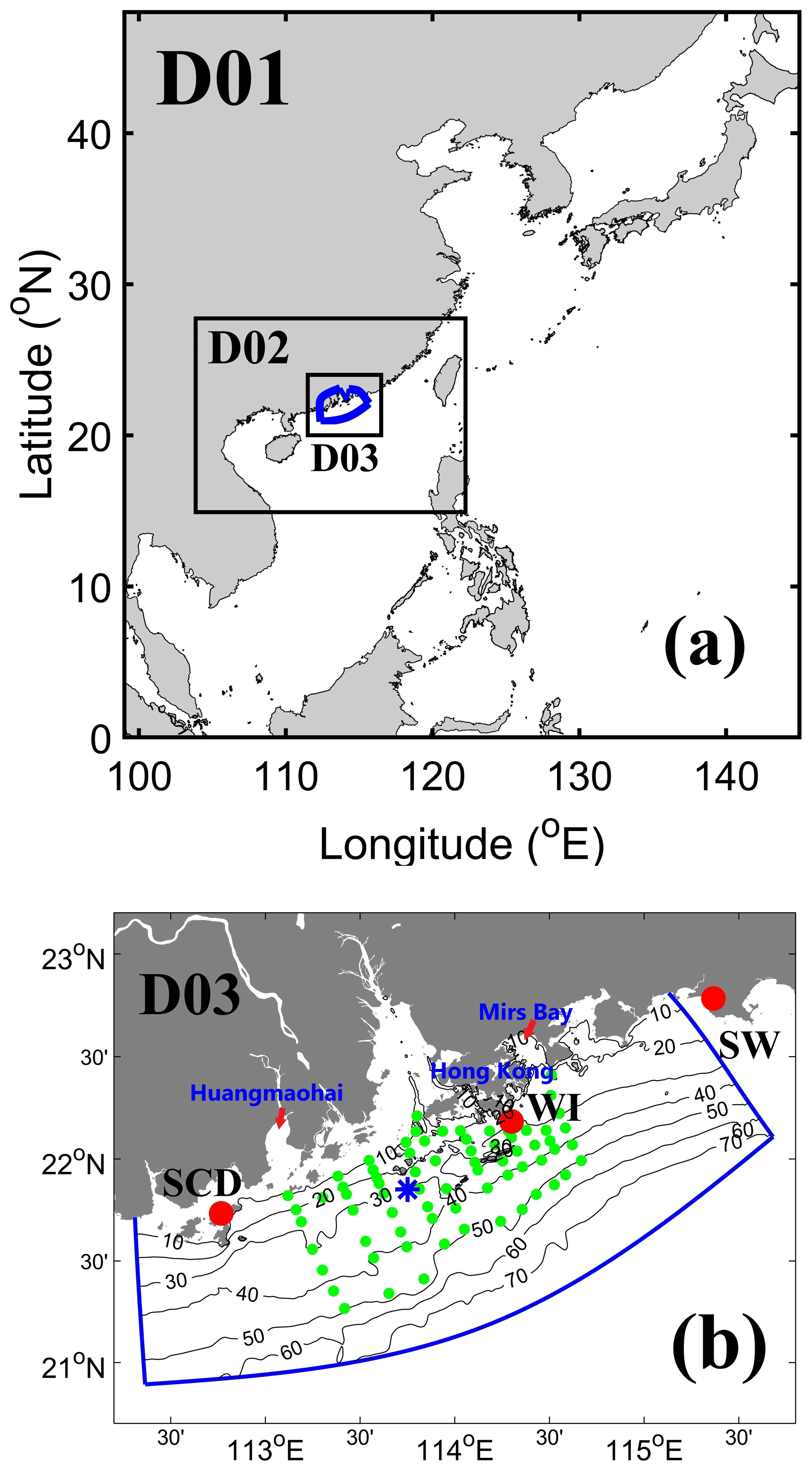
Figure 1(a) The model domains of the WRF and PRE ocean models. The blue-outlined area denotes the domain of the PRE ocean model. (b) The inner domain (D03) of the WRF model and the domain of the PRE ocean model with bathymetry (in units of meters, black contour lines). The red dots indicate weather observation stations at Shanwei (SW), Shangchuan Dao (SCD), and Waglan Island (WI). The green dots denote the sampling stations of conductivity–temperature–depth (CTD) during the cruise. The blue star indicates the location of the buoy.
2.3 Observations for validation
We used hourly surface wind and temperature data at weather stations around the PRE obtained from the Hong Kong Observatory (HKO) and the Integrated Surface Database (ISD; https://www.ncei.noaa.gov/products/land-based-station/integrated-surface-database, last access: 16 July 2023), provided by the National Centers for Environmental Information (NCEI) and the National Oceanic and Atmospheric Administration (NOAA) to validate the atmospheric forcing.
We used conductivity–temperature–depth (CTD) data collected during a cruise survey from 13 to 21 July 2017 to validate the ocean model. The in situ salinity and temperature were measured using a well-calibrated Sea-Bird SBE 25 CTD profiling system. The measurement stations were located along the transects in the PRE and over the adjacent shelf (Fig. 1b). Profiles were extracted from the model results in the corresponding locations for validation against the CTD data. Simultaneously, we conducted time-series measurements of currents using a buoy mooring located south of Hong Kong Island (Fig. 1b).
3.1 Atmosphere model validation
We compared wind vectors and air temperature results from the atmospheric model to observations from the HKO and ISD. Figure 2 shows the alongshore and cross-shore winds and air temperature at the Shanwei (SW), Waglan Island (WI), and Shangchuan Dao (SCD) stations from the observations, the ERA-Interim dataset, and the WRF model from 11 to 23 July 2017. The alongshore and cross-shore components of the wind vectors are approximately parallel and perpendicular to the coastline, respectively. A negative value of alongshore wind indicates a downwelling-favorable wind. Comparisons with observations at these three stations showed that the alongshore wind was the weakest at SW located to the east of the PRE and strongest at WI outside the PRE (Fig. 2), suggesting that the wind was highly variable along the coast. This spatial variability in the wind forcing induced by topography was erroneously omitted in the WL-OBS experiment, where uniform wind forcing was applied. Consequently, the wind forcing in the WL-OBS experiment was overestimated in comparison to the observed data.
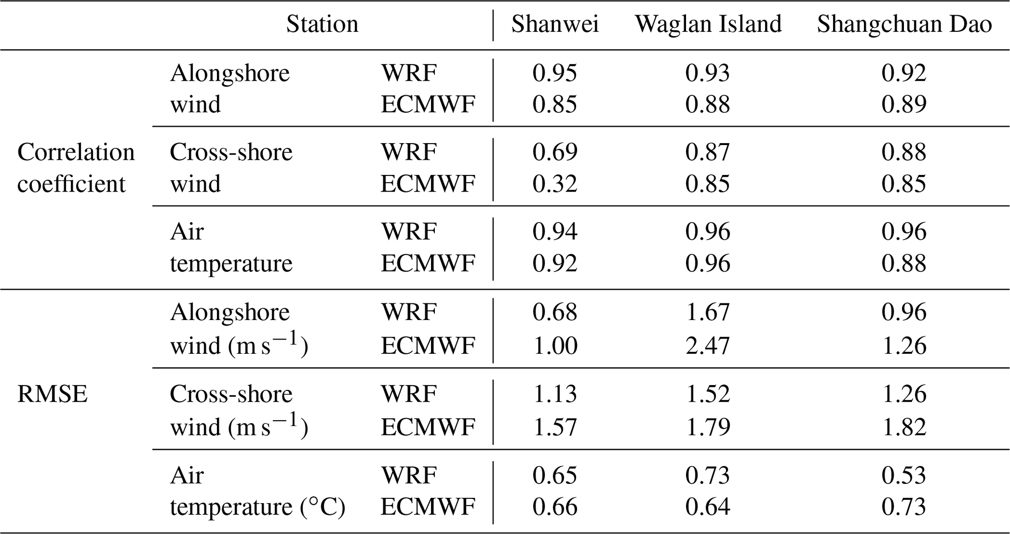
At SW, the alongshore wind from ECMWF (ERA-Interim data) overestimated the downwelling-favorable wind on 16 July (Fig. 2a), but it was underestimated at WI (Fig. 2d). The low resolution of the ERA-Interim dataset resulted in a similar magnitude and direction of the near-surface wind field at all stations. However, at WI, the intensities of the alongshore winds from the WRF model were stronger and closer to observations, indicating a better agreement between the high-resolution modeled winds and observations. The alongshore winds at the SCD station were similar between the ERA-Interim data and WRF, but the biases of cross-shore wind from the ERA-Interim data were enlarged (Fig. 2h). Overall, the high-resolution WRF model improved the simulation of cross-shore winds and agreed better with the observations at all three observation stations (Fig. 2b, e, h). The root-mean-square errors (RMSEs) of the alongshore and cross-shore winds from the WRF model were smaller than those from the ERA-Interim data for the three stations (Table 1). In addition, the correlation coefficients of the alongshore and cross-shore winds for the WRF model were more significant.
The air temperature at WI dropped from nearly 30 ∘C on 11 July to ∼ 25 ∘C on 17 July and then gradually increased to 30 ∘C again (Fig. 2c). Both the ERA-Interim data and WRF model results accurately reproduced this synoptic process, but the low-resolution ERA-Interim data overestimated the air temperature at SCD (Fig. 2i). The RMSE of the air temperature at SW was similar, but it was smaller at SCD for the high-resolution WRF result (Table 1). The correlation coefficient of air temperature was more significant in the high-resolution WRF model.
Overall, the reanalysis provided an unrealistic wind pattern in the coastal region, while a dynamical downscaling using a high-resolution atmosphere model was necessary to accurately capture the observed spatial variability in atmospheric circulation. The high-resolution atmospheric model improved the representations of wind vectors and air temperature, with lower RMSE and higher correlation coefficients of wind and temperature, respectively.
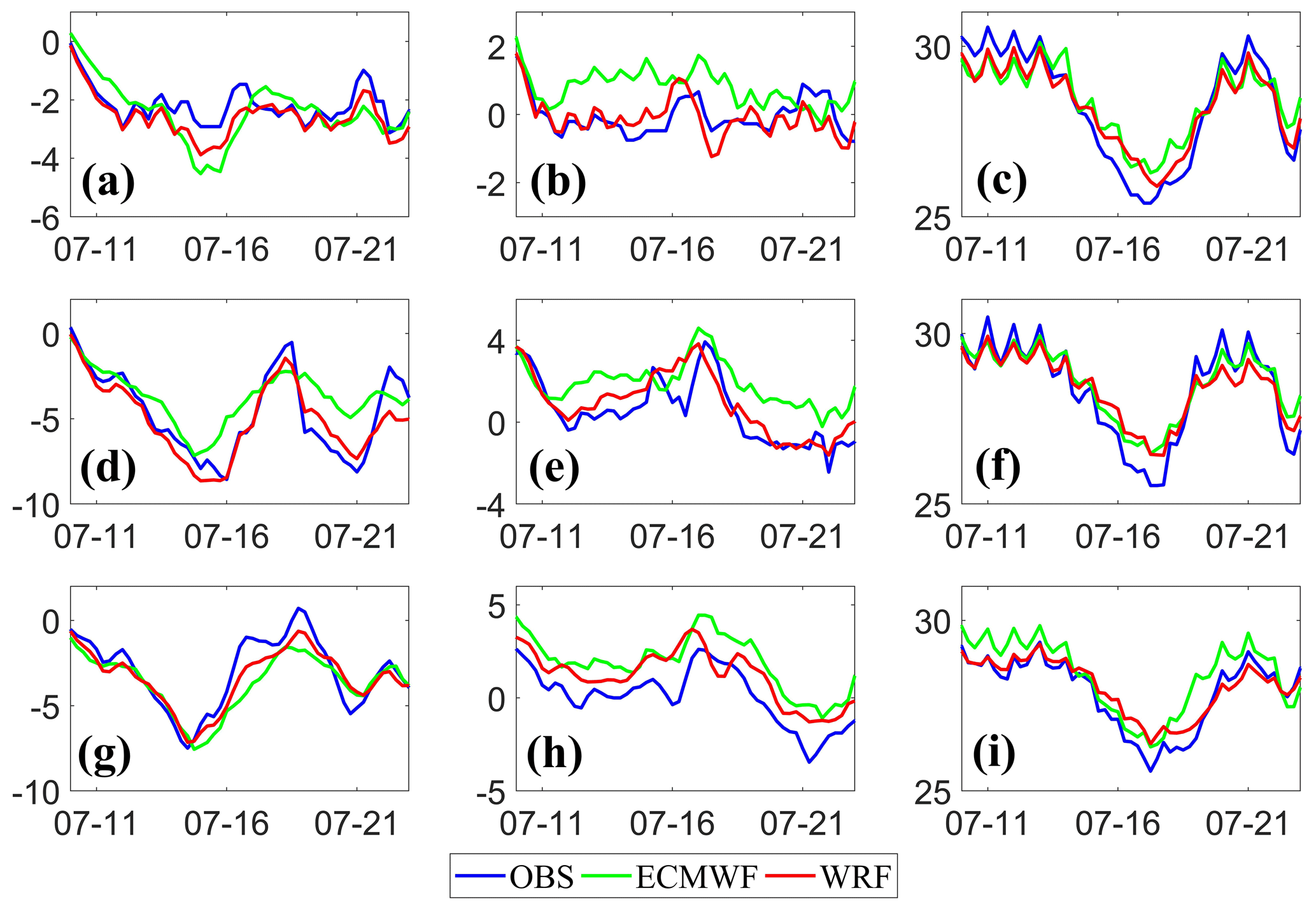
Figure 2Comparisons of (a, d, g) alongshore and (b, e, h) cross-shore winds (m s−1) and (c, f, i) air temperature (∘C) of the observations, ERA-Interim data from ECMWF, and WRF model at the Shanwei (a, b, c), Waglan Island (d, e, f), and Shangchuan Dao (g, h, i) stations. A negative value of the alongshore wind indicates a downwelling-favorable wind. A 24 h high-frequency filter has been applied to the data.
Table 1Correlation coefficients and RMSEs of alongshore and cross-shore winds and air temperature from the ERA-Interim data and WRF model at the atmospheric observation stations.
3.2 Ocean model validation
We used the horizontal map of temperature and salinity RMSEs derived from the data in the sampling stations to assess the performance of the ocean model under different atmospheric forcings (Fig. 3). The RMSEs of salinity and temperature of the water column at the CTD observation stations in the WL-OBS experiment are shown in Fig. 3a and 3e, respectively.
The larger RMSEs of temperature primarily occurred near the mouth of the estuary and in the offshore region over the shelf in the WL-OBS experiment (Fig. 3a). The differences in temperature RMSEs between the LR-ERAI and WL-OBS experiments showed that the ocean model forced by the ERA-Interim data significantly reduced the RMSEs of temperature at most stations (Fig. 3b), especially in offshore waters, indicating the importance of spatial variability in wind forcing. When the ocean model was driven by the high-resolution wind forcing (HR-WRFW experiment), the RMSEs of temperature were further reduced in the offshore region (Fig. 3c). Along with the high-resolution heat flux forcing, the differences in temperature RMSEs were negative at most stations (Fig. 3d), particularly near the coast, showing that the minimum RMSEs of temperature can be obtained in the HR-WRFA experiment. However, the RMSEs and correlation coefficient of water temperature suggested that the overall improvements in the WL-OBS, LR-ERAI, and HR-WRFW experiments were limited due to the use of the same low-resolution surface heat flux forcing (Table 2). However, application of the concurrent high-resolution surface heat flux forcing and wind forcing reduced RMSEs of temperature, and the correlation coefficient of temperature was increased in the HR-WRFA experiment.
In the WL-OBS experiment, the RMSEs of salinity at the stations were larger in the western coastal waters, where dynamical variability was most intense due to the combined forcings of freshwater discharge, tides, and winds. The RMSEs of salinity were relatively small in the offshore waters (Fig. 3e). The RMSEs of salinity increased outside the estuary but decreased on the western side when the ocean model was forced by the ERA-Interim data (Fig. 3f). Applying high-resolution wind forcing in the HR-WRFW experiment led to a decrease in the RMSEs of salinity in the shelf region (Fig. 3g) due to better simulation of the wind-driven current. The salinity RMSEs were reduced at most stations in the HR-WRFA experiment (Fig. 3h) as well. Overall, the RMSEs and correlation coefficient of salinity were comparable in the LR-ERAI and WL-OBS experiments, with higher RMSEs and lower correlation coefficients. However, the RMSEs of salinity were significantly reduced in the HR-WRFW experiment and further decreased in the HR-WRFA experiment (Table 2). The correlation coefficient of salinity also increased when using high-resolution atmospheric forcing.
Table 2RMSEs and correlation coefficients of water temperature and salinity in the CTD observations from the WL-OBS, LR-ERAI, HR-WRFW, and HR-WRFA experiments.
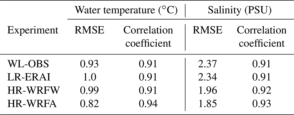
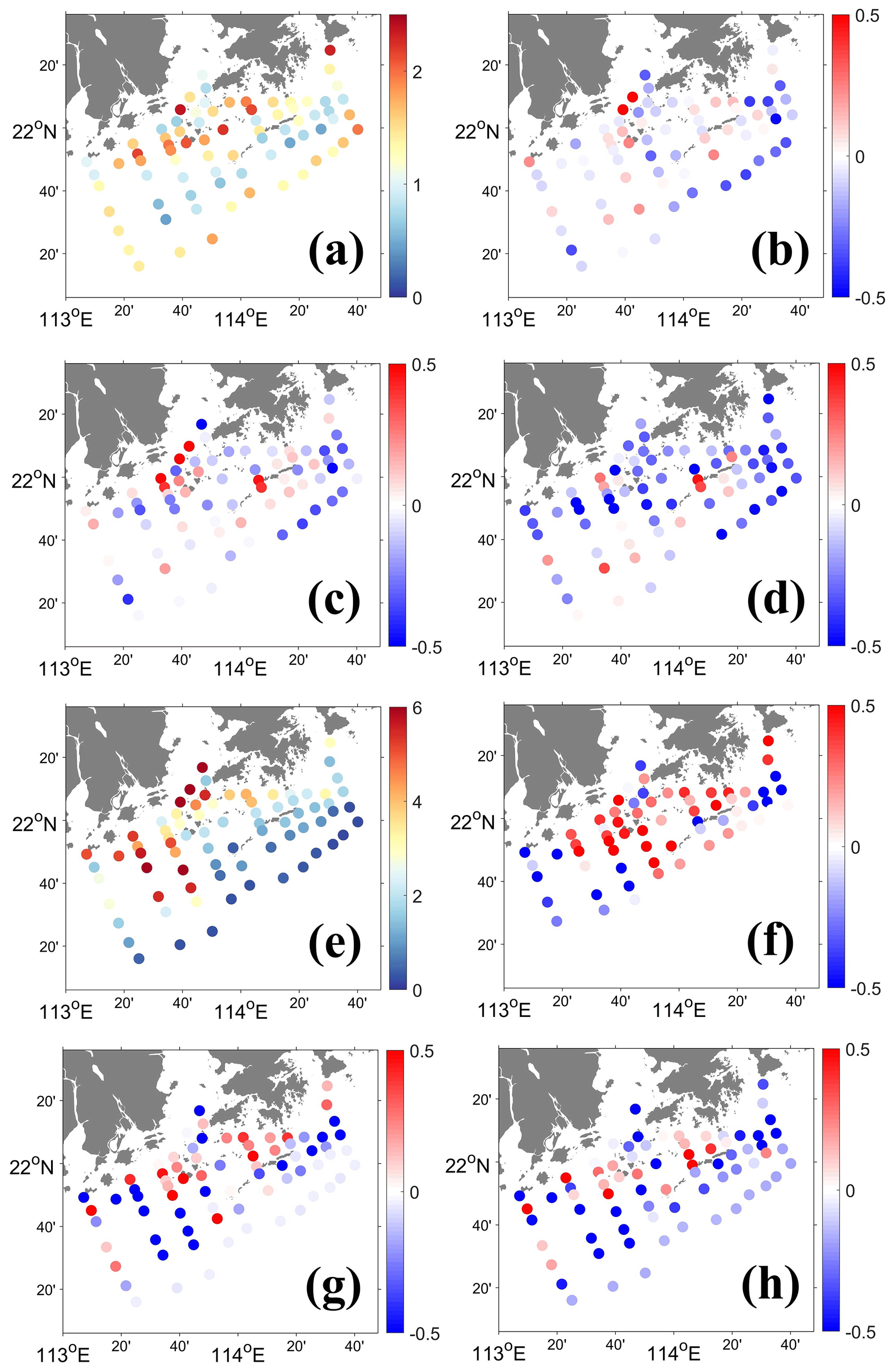
Figure 3Horizontal map of RMSEs for (a) temperature (∘C) of the water column at the CTD stations in the WL-OBS experiment. The differences in RMSE of temperature from (b) the LR-ERAI minus WL-OBS, (c) the HR-WRFW minus LR-ERAI, and (d) the HR-WRFA minus HR-WRFW experiments. Horizontal map of RMSEs for (e) the salinity (PSU) of the water column at the CTD stations in the WL-OBS experiment. The differences in RMSE of salinity from (f) the LR-ERAI minus WL-OBS, (g) the HR-WRFW minus LR-ERAI, and (h) the HR-WRFA minus HR-WRFW experiments.
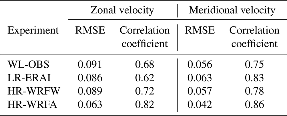
The time series of depth-averaged zonal and meridional velocities measured by the moored current meters were compared with the results from the different experiments (Fig. 4). The recorded depth-averaged zonal and meridional velocities showed extensive fluctuations under a downwelling-favorable wind. Comparison with the results from the different experiments revealed that the biases of currents were larger in the WL-OBS and LR-ERAI experiments. However, using high-resolution atmospheric forcing decreased the biases of currents in the HR-WRFW and HR-WRFA experiments, resulting in better agreement with the observations. The correlation coefficient between the observed and simulated zonal velocity improved from 0.68 in the WL-OBS experiment to 0.82 in the HR-WRFA experiment (Table 3). The RMSE of zonal velocity was also reduced from 0.091 to 0.063 m s−1. The HR-WRFA experiment had the highest correlation coefficient and lowest RMSE for the meridional velocity.
In summary, the high-resolution atmospheric model more accurately captured the local dynamic effects induced by small-scale physical processes and terrain and simulated the wind better. The improved atmospheric forcing significantly improved the accuracy of simulated coastal currents and, consequently, the associated surface water temperature and salinity.
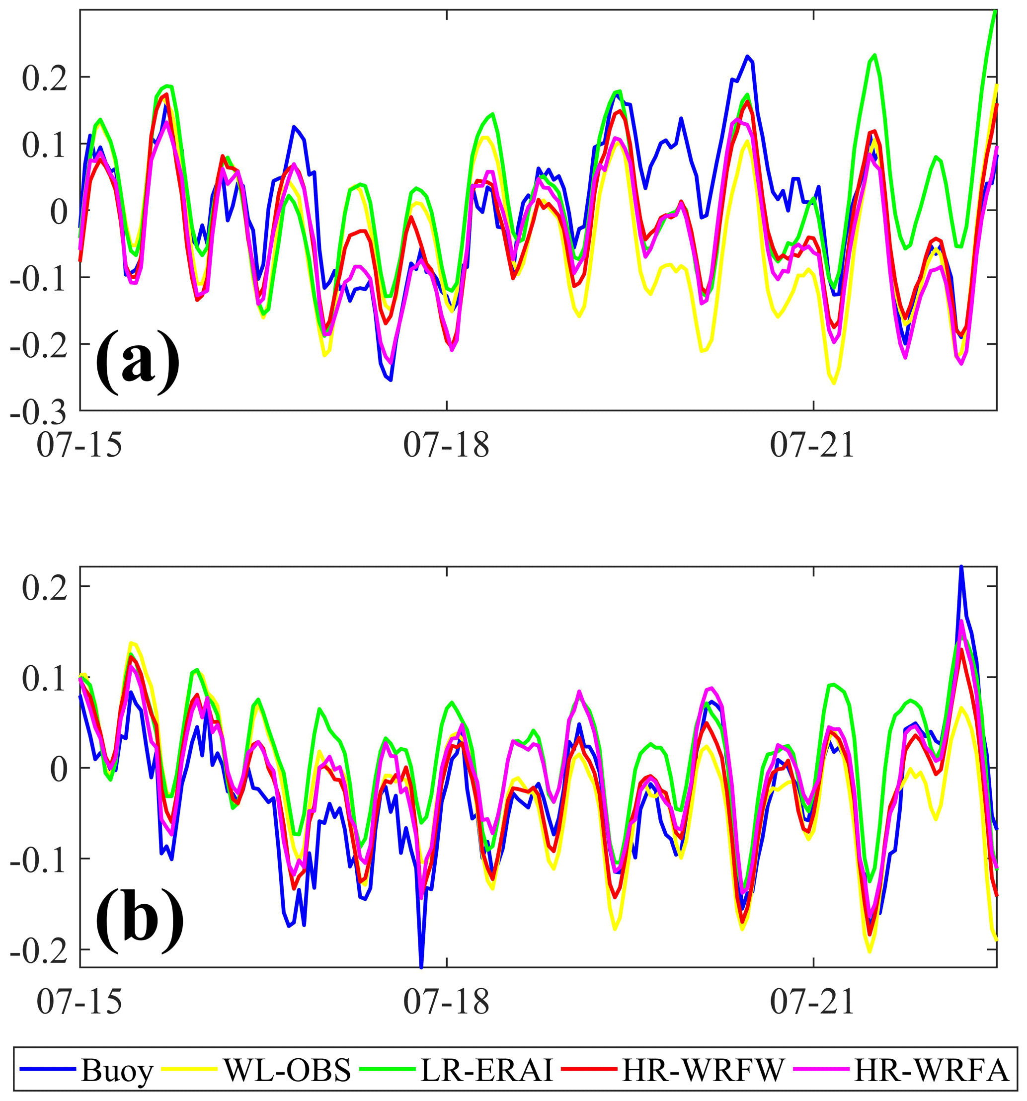
Figure 4Time series of depth-averaged (a) zonal and (b) meridional velocities (m s−1) at the buoy location from the buoy observations and the WL-OBS, LR-ERAI, HR-WRFW, and HR-WRFA experiments.
At the beginning of the field cruise in the PRE region, a moderate upwelling-favorable wind was observed from 6 to 10 July 2017. This was followed by a prolonged period of downwelling-favorable wind starting from 11 July. In each of our four experiments here, our main focus was to study the response of coastal ocean circulation to the downwelling-favorable wind, which occurred between 11 and 21 July 2017.
4.1 Simulated characteristics of shelf currents
The dynamics of coastal ocean circulation are greatly influenced by wind stress and wind stress curl, which play a crucial role in the upwelling and downwelling of water. The time-averaged wind stress and wind stress curl used in the WL-OBS, LR-ERAI, HR-WRFW, and HR-WRFA experiments are shown in Fig. 5 when the downwelling-favorable wind prevailed from 11 to 21 July. The different resolutions of wind data revealed variations in intensity and patterns in the wind stress and wind stress curl structures over the PRE region. In the WL-OBS experiment, the wind forcing from the Waglan Island observation was uniformly applied throughout the region, as seen in Fig. 5a. However, the intensity of the wind stress from the ERA-Interim reanalysis data was found to be weaker than that in the WL-OBS experiment (Fig. 5b). Additionally, the alongshore wind stress was stronger in the west and weaker in the east. Furthermore, wind stress strengthened in the high-resolution WRF model (Fig. 5c), particularly over the shelf. The wind stress curl was absent in the WL-OBS experiment (not shown). However, the ERA-Interim data revealed a generally negative and spatially uniform wind stress curl over the shelf (Fig. 5d). In contrast, the high-resolution WRF model displayed a marked spatial variability and structure in the wind stress curl (Fig. 5e). The high-resolution WRF model depicted an intensification of wind stress curl near the coast, which exhibited a more detailed representation of wind stress curl variability. However, the magnitude of wind stress curl was weaker in comparison to the low-resolution ERA-Interim data (Fig. 5e).
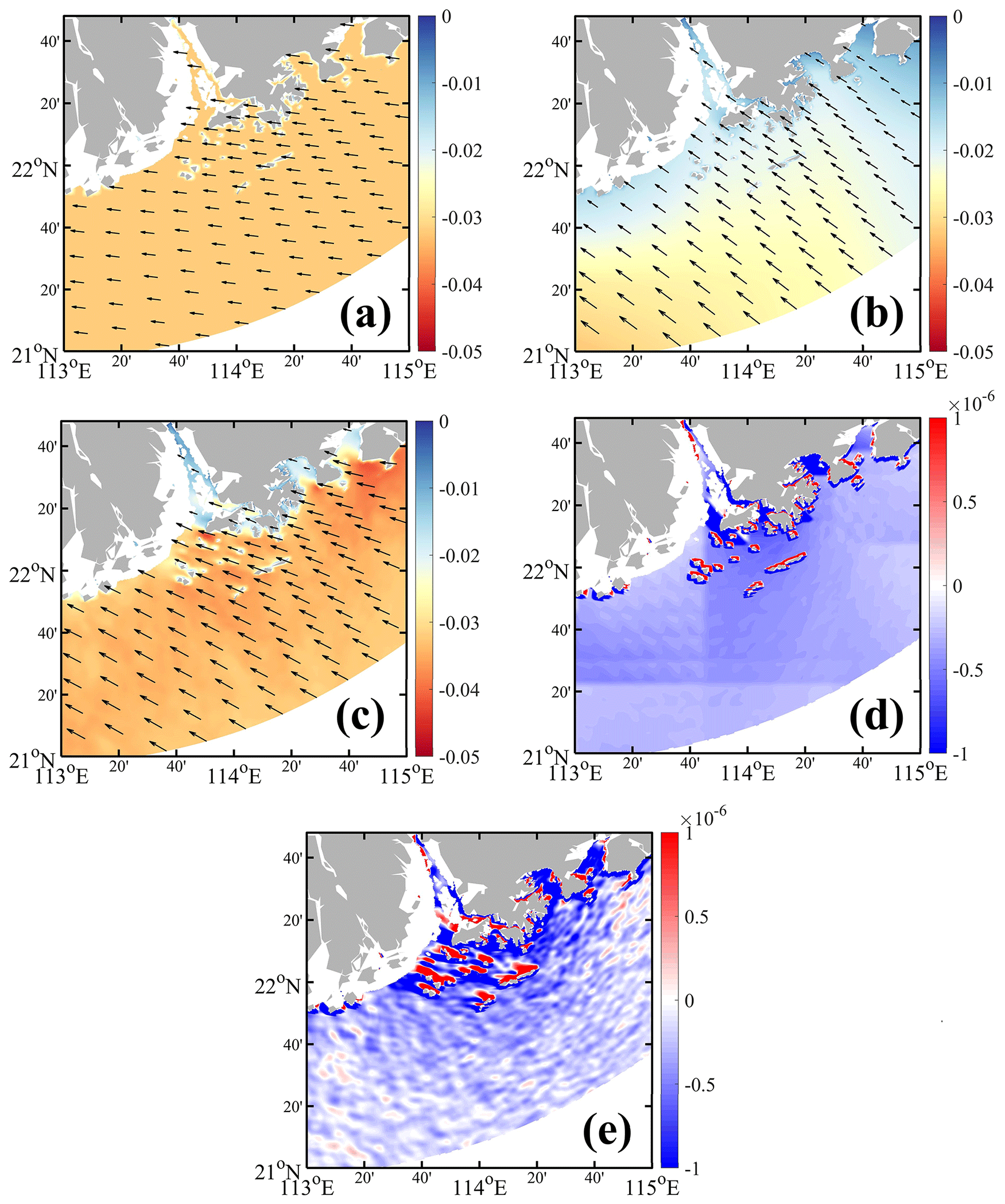
Figure 5The time-averaged wind stress (Pa) from the (a) Waglan Island observation, (b) ERA-Interim data, and (c) high-resolution WRF model during the downwelling-favorable wind from 11 to 21 July 2017. The colors show the magnitude of the alongshore wind stress. The time-averaged wind stress curl (N m−3) from the (d) ERA-Interim data and (e) WRF model during the downwelling-favorable wind from 11 to 21 July 2017.
Table 3RMSEs and correlation coefficients of depth-averaged zonal and meridional velocities (m s−1) between buoy observations and the WL-OBS, LR-ERAI, HR-WRFW, and HR-WRFA experiments.
When extensive and persistent northeasterly (downwelling-favorable) winds prevailed, the pre-existing northeast upwelling shelf currents carrying buoyant waters rapidly reverted to a southwestward flow in the surface layer (Fig. 6a). However, in the east of the PRE, the northeastward shelf currents were weakened but maintained (Fig. 6a), supported by the river plume salinity (Fig. 6e) and a cold-water belt from the upslope invasion of deep shelf water by the upwelling circulation (Fig. 7a). According to Liu and Gan (2020), an upslope invasion of the shelf waters in the east can be induced by a counter-current established by the remote effect from exchange flows in the Taiwan Strait where the southwesterly wind was persistent.
The difference in surface currents between the WL-OBS and LR-ERAI experiments suggested that the southwestward alongshore jet was weaker, but the northeastward jet was stronger in the LR-ERAI experiment due to the weaker wind stress (Fig. 6b). Furthermore, the southwestward alongshore and northeastward jets were stronger in the HR-WRFW experiment driven by high-resolution wind forcing than in the LR-ERAI experiment (Fig. 6c). When combined with the high-resolution heat forcing, water was generally warmer (Fig. 7d) and the strength of the southwestward alongshore jet was decreased in the HR-WRFA experiment; however, surface currents slightly increased over the shelf as compared with the HR-WRFW experiment.
The surface salinity in the PRE is characterized by the offshore and eastward movement of the Pearl River plume during pre-existing northeast upwelling. When the wind stress turns to downwelling-favorable winds in the WL-OBS experiment, the freshwater from the estuary is advected westward and offshore while lower-salinity water extends to the east by the northeastward jet on the eastern side (Fig. 6e). The 27 PSU surface salinity contours indicated that more freshwater was constrained on the western side of the PRE due to the stronger southwestward alongshore jet in the WL-OBS experiment (Fig. 6e) as compared to the other scenarios. The patterns of surface salinity from the HR-WRFW and HR-WRFA experiments were similar to that in the WL-OBS experiment in the west, indicating similar currents. Meanwhile, freshwater spread further eastward in the LR-ERAI experiment, suggesting the strongest eastward jet, but the eastward jets were weaker when driven by the high-resolution wind forcing in the HR-WRFW and HR-WRFA experiments.
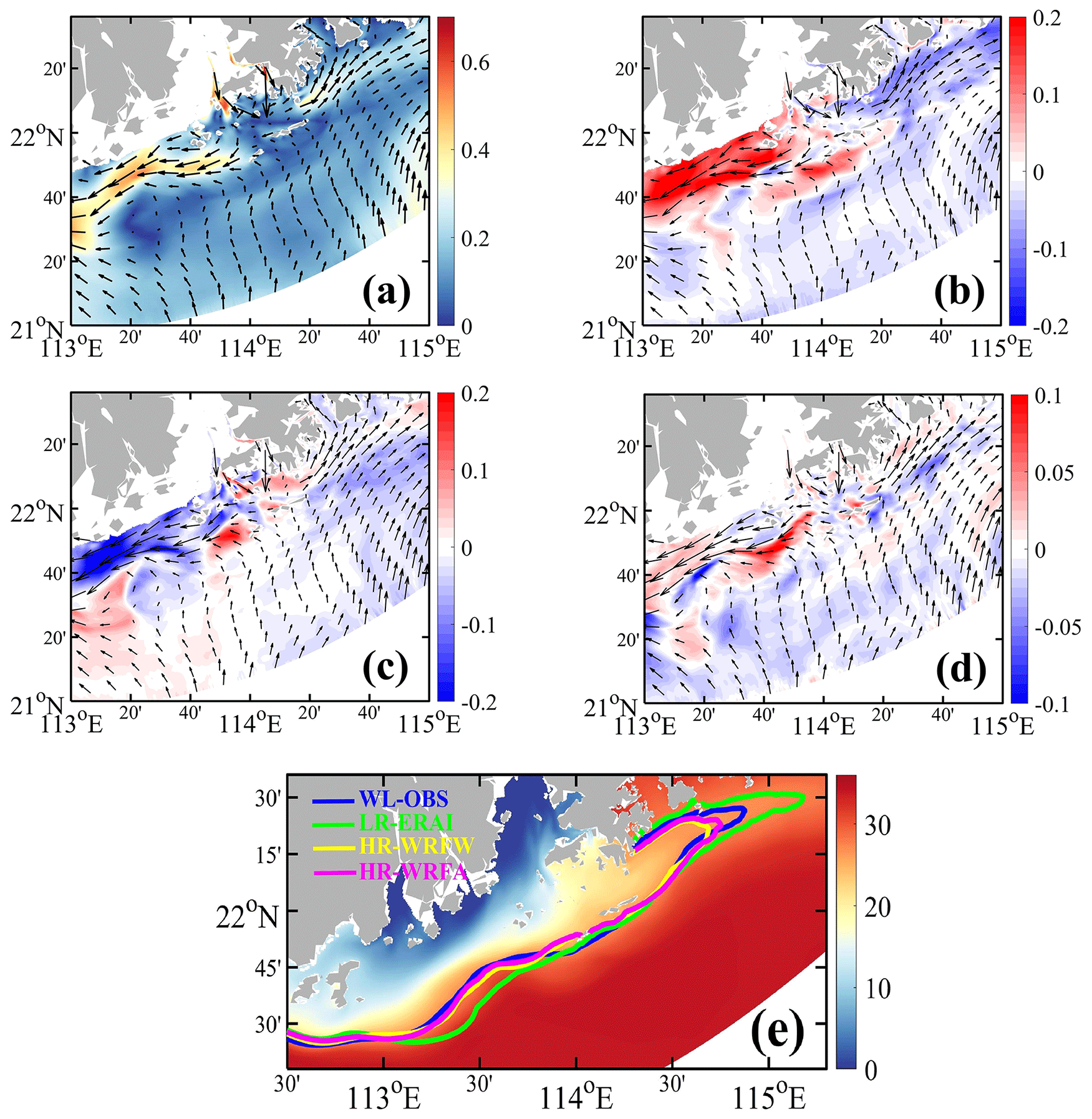
Figure 6The time-averaged surface currents (m s−1) in the (a) WL-OBS experiment during the downwelling-favorable wind from 11 to 21 July 2017. The differences in the magnitude of time-averaged surface current from (b) the WL-OBS minus LR-ERAI, (c) the LR-ERAI minus HR-WRFW, and (d) the HR-WRFW minus HR-WRFA experiments during the downwelling-favorable wind from 11 to 21 July 2017. The velocity vectors in (a)–(d) indicate the surface circulation in the WL-OBS, LR-ERAI, HR-WRFW, and HR-WRFA experiments. The colors in (a) show the magnitude of the surface circulation in the WL-OBS experiment. The colors in (b), (c), and (d) show the difference in the magnitude of the surface circulation. The time-averaged sea surface salinity (PSU) in the (e) WL-OBS experiment during the downwelling-favorable wind and the contours of 27 PSU surface salinity in the WL-OBS, LR-ERAI, HR-WRFW, and HR-WRFA experiments are shown in (e) as blue, green, yellow, and magenta contour lines, respectively.
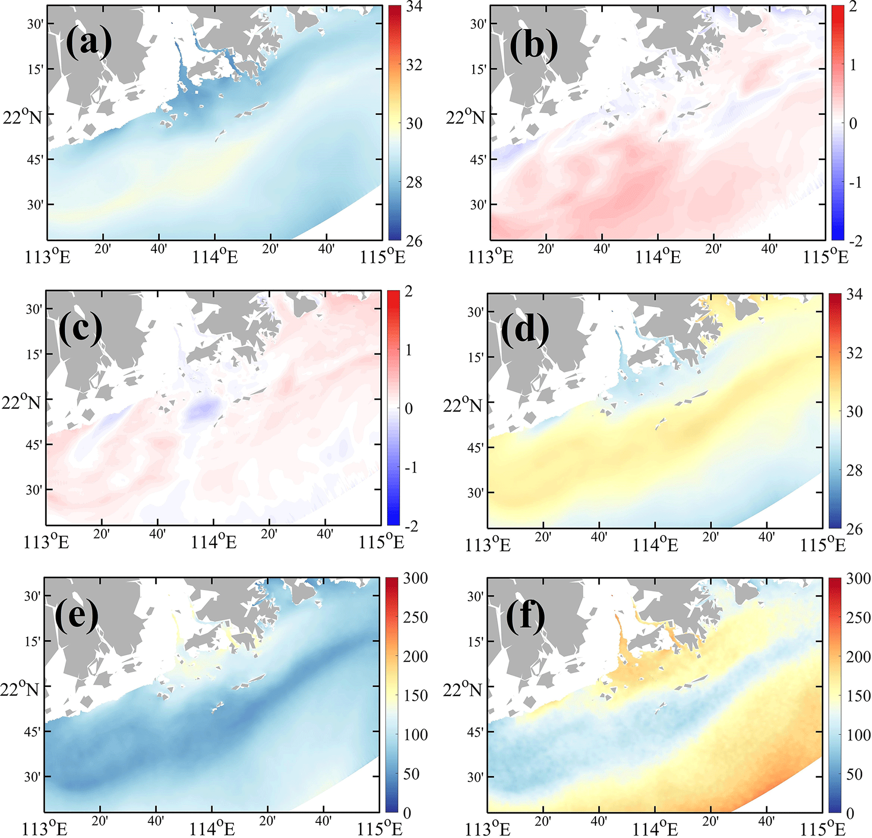
Figure 7The time-averaged SST (∘C) in the (a) WL-OBS experiment during the downwelling-favorable wind from 11 to 21 July 2017. The differences in time-averaged SST from (b) the LR-ERAI minus WL-OBS, (c) the HR-WRFW minus LR-ERAI, and (d) the HR-WRFA minus HR-WRFW experiments during the downwelling-favorable wind from 11 to 21 July 2017. The time-averaged net heat flux (W m−2) in the (e) HR-WRFW and (f) HR-WRFA experiments during the downwelling-favorable wind from 11 to 21 July 2017. A downward flux is positive (heating).
The SST distribution showed a noticeable upwelling circulation, as evidenced by the cold-water belt to the east of the PRE under downwelling-favorable winds (Fig. 7a). Despite the heat flux forcing being the same in the WL-OBS, LR-ERAI, and HR-WRFW experiments, the near-surface water was cooler in the LR-ERAI experiment (Fig. 7b), showing the impacts of wind and current on the SST. The difference in SST between the LR-ERAI and HR-WRFW suggested that SST was slightly decreased when driven by the high-resolution wind forcing (Fig. 7c) due to increased vertical mixing induced by strengthened wind stress. The positive net heat flux from the ERA-Interim data was smaller than that from the high-resolution WRF model (Fig. 7e, f) due to the underestimation of net downward shortwave radiation in the low-resolution global reanalysis data (figure not shown), resulting in an increased SST in the HR-WRFA experiment (Fig. 7d). The warmer water can cause the ocean surface to expand and its density to decrease, which in turn can cause the water to rise and affect the pressure gradient, leading to changes in ocean circulation.
We examined the cross-isobath components of depth-averaged bottom velocities over the 10 to 50 m isobaths by projecting the simulated velocities onto the cross-isobath direction to illustrate the response of the cross-shelf exchanges to different atmospheric forcing during the downwelling-favorable wind (Fig. 8). We defined the orientation of the isobath in the computational domain as the inverse tangent of the northward and eastward gradients of the topography. A positive value represents an onshore transport, while a negative value indicates an offshore transport, and both are perpendicular to the isobaths. Based on the pattern of the water exchange in different regions of our model domain, we selected two regions around the PRE for discussion (Fig. 8a). In the west, we defined Region W to be on the shelf from the 30 to 50 m isobaths. Region E was in the east from the 20 to 50 m isobaths. However, due to the complexity of the complex topography and islands in the central region, we exclude a discussion of cross-isobath transport for that area.
The patterns of depth-averaged and bottom cross-isobath transport were qualitatively similar in the four experiments, and here only the results from the HR-WRFW experiments are shown (Fig. 8a and b). Cross-shelf exchanges of the shelf and coastal waters mainly occurred over the irregular topography near the Huangmaohai Estuary in the west (Region W) and over a shallow trough off Mirs Bay in the east (Region E). These water exchanges were intensified at the locations where the isobaths meander, as previously reported by Liu et al. (2020). When a downwelling-favorable wind prevailed after an upwelling-favorable wind, the depth-averaged cross-isobath transports exhibited a net offshore transport for Region W and an onshore invasion on the eastern side for Region E (Fig. 8a), resulting in a lower temperature around Hong Kong Island (Fig. 7a). Meanwhile, the bottom cross-isobath transport displayed similar patterns to the depth-averaged cross-isobath transport (Fig. 8b). The domain- and depth-averaged cross-isobath transport suggested that the depth-averaged cross-isobath transport in the LR-ERAI experiment was strongest for both onshore and offshore transport. The cross-isobath transport was slightly weaker in the HR-WRFA experiment driven by the high-resolution heat forcing compared with the HR-WRFW experiment (Fig. 8c). The depth-averaged cross-isobath offshore transport in Region W was weakest in the WL-OBS experiment, but the onshore transport in Region E was similar to the HR-WRFW and HR-WRFA experiment (Fig. 8c). Similarly, the bottom onshore and offshore transports were strongest in the LR-ERAI experiment, but the intensities of bottom onshore and offshore transport were slightly stronger in the HR-WRFA experiment compared with the HR-WRFW experiment (Fig. 8d). In the next section, we discuss the underlying dynamics of the changing transports in the different experiments.
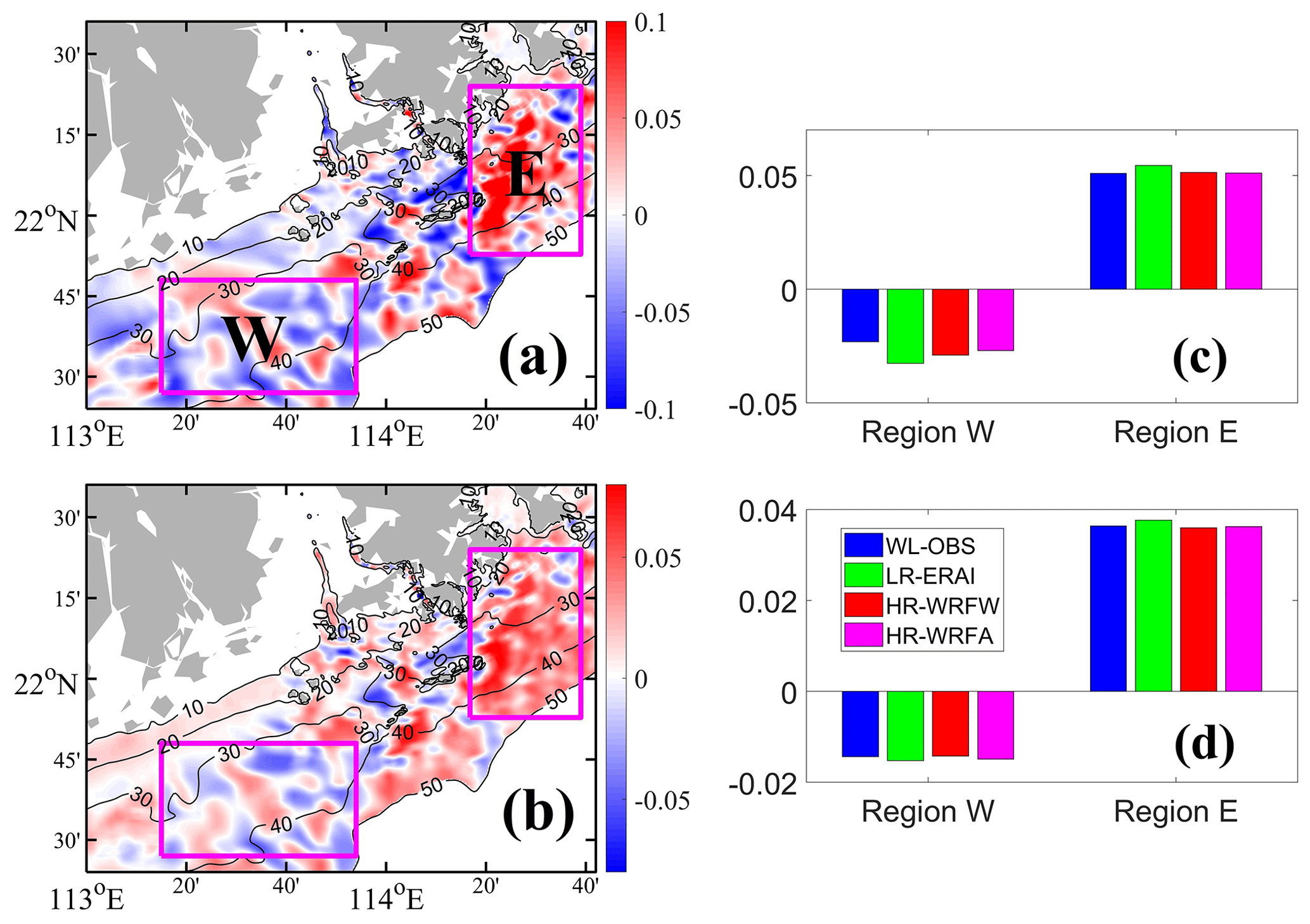
Figure 8The time average of (a) depth-averaged and (b) bottom cross-isobath velocities (m s−1) in the HR-WRFW experiment during the downwelling-favorable wind from 11 to 21 July 2017. Time and domain average of the (c) depth-averaged and (d) bottom cross-isobath velocity (m s−1) for Region W and Region E in the WL-OBS, LR-ERAI, HR-WRFW, and HR-WRFA experiments during the downwelling-favorable wind from 11 to 21 July 2017. A positive value represents an onshore transport, while a negative value indicates an offshore transport, and both are perpendicular to the isobaths.
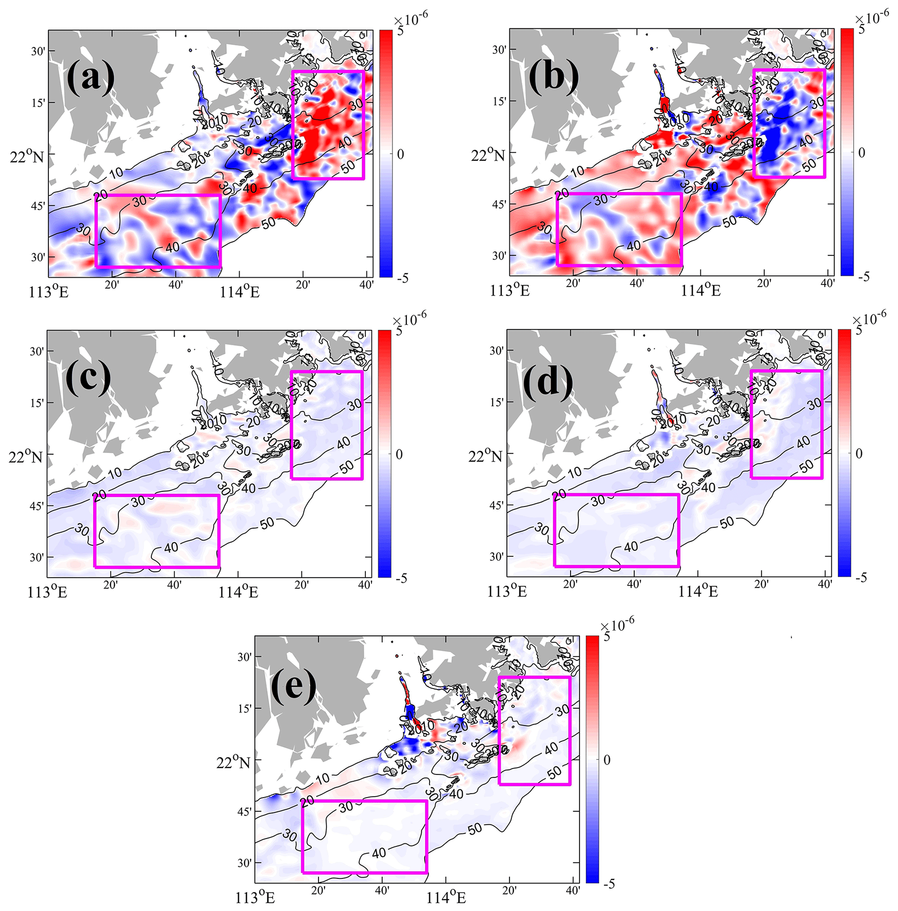
Figure 9Horizontal maps of time-averaged along-isobath (a) Coriolis force (COR), (b) pressure gradient force (PGF), (c) surface stress (SSTR), (d) frictional bottom stress (BSTR), and (e) horizontal nonlinear advection (HADV) (ms−2) in the HR-WRFW experiment during the downwelling-favorable wind from 11 to 21 July 2017.
To better understand the impact of high-resolution wind and heat forcings on the dynamic processes of the cross-isobath transport around the PRE, we use term balances in the depth-averaged momentum and vorticity equations. This enables us to examine the dynamic characteristics controlling the processes of cross-isobath transport.
6.1 Dynamics of cross-isobath transport
We analyzed the forcing mechanisms involved in the cross-isobath transport with the corresponding along-isobath momentum balances. The terms in the depth-averaged momentum equation were projected onto the along-isobath direction to better investigate the cross-isobath velocity. The depth-averaged along-isobath momentum equation is expressed as
where the subscript y* denotes the momentum in the along-isobath direction. The and terms are the depth-averaged velocities in the cross-isobath and along-isobath directions, respectively. The reference density and coefficient of horizontal viscosity are represented by ρ0 and Kh, respectively. The terms in Eq. (1) are acceleration (ACCEL), Coriolis force (COR), horizontal nonlinear advection (HADV), pressure gradient force (PGF), surface stress (SSTR), frictional bottom stress (BSTR), and horizontal viscosity (HVISC).
We first present time-averaged horizontal distributions of depth-averaged along-isobath momentum terms in the HR-WRFW experiment (Fig. 9) during the downwelling-favorable wind. The corresponding differences in different experiments are given in Fig. 10. The negligible contributions from the acceleration and HVISC were excluded from the following discussion. The principal balance along the isobaths in both Region W and Region E was between the COR and PGF terms (Fig. 9a, b). The contributions of SSTR, BSTR, and HADV were weaker than that of PGF, indicating that the major contributor to the cross-isobath exchanges was the along-isobath pressure gradient PGF, suggesting a geostrophic current. A positive PGF in the west indicated an offshore transport (COR), while a negative PGF in the east indicated an onshore transport (COR). A negative SSTR and negative BSTR over the shelf suggest that surface and bottom Ekman processes contributed to the onshore invasion of shelf waters, weakening the offshore transport in the west and strengthening the onshore transport in the east. SSTR and BSTR in Region W were weaker than those in Region E (Fig. 9c). HADV was weaker over the shelf but stronger in the navigational channels and around the islands, where PGF was mainly balanced by HADV (Fig. 9b, e), suggesting gravitational circulation.
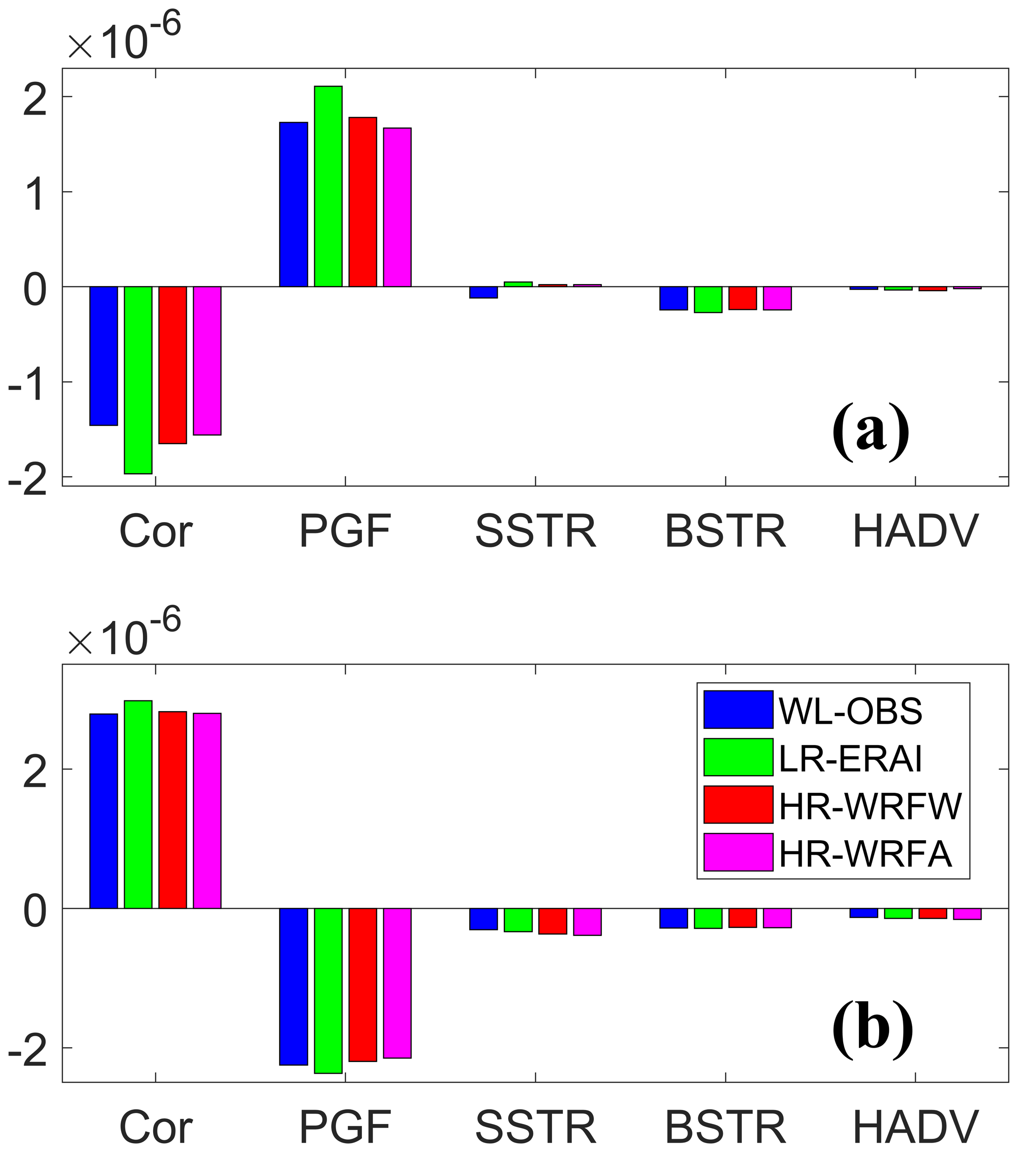
Figure 10Time and domain average of along-isobath COR, PGF, SSTR, BSTR, and HADV (ms−2) in Eq. (1) for the WL-OBS, LR-ERAI, HR-WRFW, and HR-WRFA experiments in (a) Region W and (b) Region E during the downwelling-favorable wind from 11 to 21 July 2017.
Figure 10 shows the time and domain average of the depth-averaged along-isobath momentum terms in Region W and Region E for the WL-OBS, LR-ERAI, HR-WRFW, and HR-WRFA experiments during the downwelling-favorable wind. Similarly, the major balance along the isobaths in both Region W and Region E was between COR and PGF in all four experiments. The intensity of the along-isobath PGF plays a significant role in determining the strength of cross-isobath transport in both Region W and Region E. Stronger along-isobath PGF in the LR-ERAI experiment resulted in stronger cross-isobath transport in both Region W and Region E. However, when high-resolution wind forcing was applied in the HR-WRFW experiment, the intensities of the along-isobath PGF decreased in both Region W and Region E. When using the high-resolution heat forcing in the HR-WRFA experiment, the intensities of PGF were further reduced. The impact of SSTR on offshore transport in Region W varied in different experiments. In the WL-OBS experiment, using a spatially uniform wind forcing (SSTR) weakened the offshore transport. In contrast, SSTR intensified the offshore transport in Region W in the LR-ERAI, HR-WRFW, and HR-WRFA experiments, which were driven by spatially variable winds. In Region W, the effect of SSTR on offshore transport in the LR-ERAI experiment was weaker than those in the HR-WRFW and HR-WRFA experiments. However, in Region E, the effect of SSTR on the onshore transport was stronger in the HR-WRFW and HR-WRFA experiments compared with the LR-ERAI experiment due to enhanced wind stress. HADV had a minimal impact on the cross-isobath transport in both Region W and Region E across all four experiments. BSTR had the strongest influence in the LR-ERAI experiment due to stronger bottom currents. Overall, the cross-isobath transport was primarily determined by the along-isobath PGF and adjusted by the SSTR and BSTR induced by the variable atmospheric forcing.
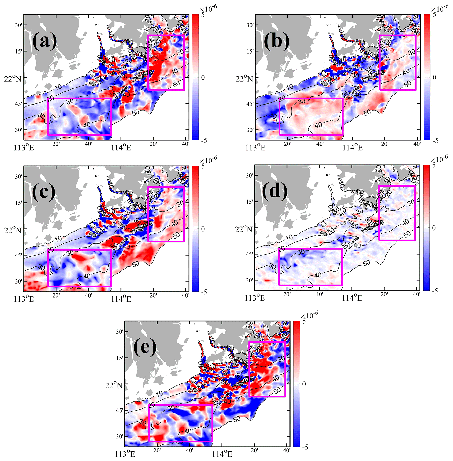
Figure 11Horizontal maps of time-averaged (a) bottom along-isobath PGF, (b) joint effect of baroclinicity and relief (JEBAR), (c) bottom stress curl (BSC), (d) surface stress curl (SSC), and (e) relative vorticity advection (RVA) (ms−2) in the HR-WRFW experiment during the downwelling-favorable wind from 11 to 21 July 2017. A positive value represents an onshore transport, while a negative value indicates an offshore transport, and both are perpendicular to the isobaths.
6.2 Dynamics of along-isobath PGF
We identified that the cross-isobath exchange in the study area is primarily controlled by the geostrophic current from PGF. The cross-isobath velocity also showed great similarity to that in the bottom boundary layer in accordance with the small Ekman number. The impact of different atmospheric forcings on the formation mechanism of this along-isobath PGF (PGF) is further explained in the following sections, utilizing the depth-integrated vorticity equation proposed in Gan et al. (2013) and Liu et al. (2020) (Eq. 2):
where subscripts x* and y* denote partial differentiation in the perpendicular and along-isobaths directions, respectively. In the water column, the along-isobath PGF can be further decomposed into the joint effect of baroclinicity and relief (JEBAR) and pressure gradient force in the bottom boundary layer PGF (Mertz and Wright, 1992), as shown in Eq. (3):
PGF is governed by JEBAR; the net stress curl is jointly governed by the bottom stress curl (BSC), the surface stress curl (SSC), and the nonlinear relative vorticity advection (RVA), as well as the gradient of momentum flux (GMF). GMF can be neglected here due to its limited contribution compared with the other processes.
Figure 11 displays the time-averaged horizontal distributions of the bottom along-isobath PGF (PGF), JEBAR, BSC, SSC, and RVA terms in the HR-WRFW experiment during the downwelling-favorable wind. The spatial distribution of PGF was similar to that of PGF (Fig. 9a), which controlled the cross-isobath transports of shelf waters. JEBAR, caused by the baroclinicity of the buoyant plume and shelf waters, dominated the cross-isobath velocities near the coast and two deep channels (Fig. 11b). JEBAR strengthened the onshore transport in Region E but weakened the offshore transport in Region W. RVA, due to the combined effect of the shelf current and the along-isobath variation in the relative vorticity, was the major contributor to the water transport over the shelf (Fig. 11e). BSC distribution was similar to that of RVA (Fig. 11c), as the second-largest contributor to the cross-isobath exchanges of waters. SSC was smaller than other terms and systematically facilitated the cross-isobath transport of shelf waters in the water column (Fig. 11d). RVA, BSC, and JEBAR regulated the cross-isobath exchanges of waters in Region W. In Region E, it was mainly sourced from RVA and partially offset by BSC over the trough near the entrance of Mirs Bay.
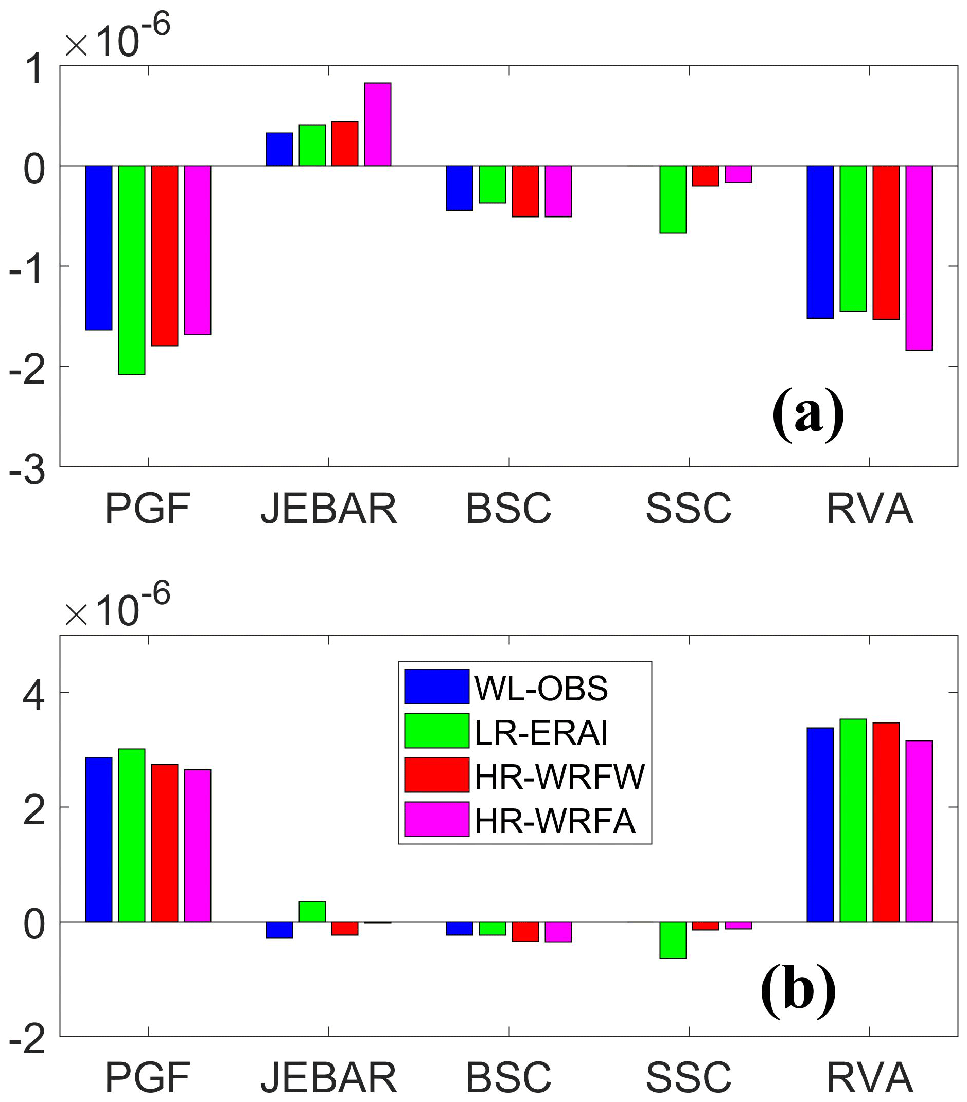
Figure 12Time and domain average of along-isobath PGF, JEBAR, BSC, SSC, and RVA (ms−2) in Eq. (2) for the WL-OBS, LR-ERAI, HR-WRFW, and HR-WRFA experiments for (a) Region W and (b) Region E during the downwelling-favorable wind from 11 to 21 July 2017. A positive value represents an onshore transport, while a negative value indicates an offshore transport, and both are perpendicular to the isobaths.
The domain averages of the along-isobath PGF, JEBAR, BSC, SSC, and RVA terms in Region W and Region E for the WL-OBS, LR-ERAI, HR-WRFW, and HR-WRFA experiments are shown in Fig. 12 to further identify the impacts of different atmospheric forcing on the different components of forming the along-isobath PGF. A positive value represents an onshore transport, while a negative value indicates an offshore transport, and both are perpendicular to the isobaths. The net stress curl (BSC and SSC) and RVA contribute to the offshore transport in Region W for all the experiments (Fig. 12a). In the HR-WRFA experiment driven by high-resolution wind and heat forcing, RVA was strongest, but it was offset by a large JEBAR, resulting in a weaker along-isobath PGF and offshore transport. The LR-ERAI experiment had the weakest BSC and RVA but the strongest SSC, leading to the strongest along-isobath PGF in Region W. The high-resolution WRF model tended to weaken the domain-averaged SSC but enhanced BSC, RVA, and JEBAR. In comparison to the LR-ERAI experiment, the HR-WRFW experiment saw an increase in JEBAR, which was further enhanced in the HR-WRFA experiment. In Region E, RVA was the major contributor in four experiments (Fig. 12b). The LR-ERAI experiment had the strongest RVA, leading to a strong along-isobath PGF and cross-isobath transport. Similarly, SSC decreased and BSC increased in the HR-WRFW and HR-WRFA experiments driven by high-resolution wind forcing. The HR-WRFA experiment, which involved stronger net heat flux forcing, resulted in a weaker RVA. This was further offset by a larger BSC, leading to a weaker along-isobath PGF and cross-isobath transport.
Overall, the high-resolution WRF model weakened SSC and strengthened BSC. BSC and SSC are similar in the HR-WRFW and HR-WRFA experiments due to the similar wind forcing. The along-isobath PGF was influenced by the high-resolution heat forcing primarily through JEBAR and RVA processes, with JEBAR being stronger in the HR-WRFA experiment. In the HR-WRFA experiment, RVA increased in Region W with a downwelling circulation but decreased in Region E with an upwelling circulation.
Accurate representation of the surface heat budget and momentum fluxes is essential to the boundary forcing of ocean modeling. We here investigated the variability in coastal circulation and dynamic response to spatiotemporally varying atmospheric forcing off the PRE at the onset of downwelling-favorable wind after a prevailing upwelling wind. Four numerical ocean simulations were driven by (1) the observations from the Waglan Island station using a uniform spatial distribution, (2) global reanalysis data from ECMWF, (3) high-resolution wind forcing, and (4) high-resolution atmospheric wind and heat forcing from a regional atmospheric model. Comparisons between the model results and the in situ observations suggest that the high-resolution atmospheric model significantly improved the simulation of the near-surface wind and air temperature, resulting in significant accuracy improvements in our simulations for coastal ocean currents, water temperature, and salinity.
We also performed momentum and vorticity analyses to further rationalize the response of the cross-shore exchange flows to different atmospheric forcing factors. The momentum analyses suggest that the cross-isobath exchange of water was mainly governed by the along-isobath pressure gradient force, whose magnitude was affected by the different atmospheric forcings. Compared to the simulation driven by the lower-resolution forcing, the intensity of along-isobath PGF decreased by applying the high-resolution wind and heat flux forcings, resulting in a weaker cross-isobath water exchange. The frictional bottom and surface Ekman transport play a secondary role in altering the cross-isobath exchange. The high-resolution atmospheric forcing tended to strengthen the surface Ekman transport east of the PRE but weakened it in the west.
Analyses based on the depth-integrated vorticity equations further suggest that the variability in the along-isobath PGF was jointly formed by the nonlinear advection of relative vorticity caused by the dynamic interaction between the eastward flow and variable shelf topography and the net stress curl (frictional bottom and surface stress curl). The JEBAR effect efficiently adjusted the along-isobath PGF in the west but had limited impact in the east. The horizontal distribution of these terms was regulated by different atmospheric forcing to form the exchange flows. Stronger heat flux forcing increased the nonlinear advection of relative vorticity and the JEBAR effect but decreased the surface stress curl, resulting in a decreased along-isobath PGF and weakened cross-isobath water exchange west of the PRE. However, in the east, the nonlinear advection of relative vorticity decreased, leading to a weaker cross-isobath transport. Improved high-resolution atmospheric forcing dynamically refined the formation and variability in the along-isobath pressure gradient force and the associated cross-isobath water exchange.
The numerical results presented in the figures were produced by solving equations in the Regional Ocean Modeling System (ROMS). The source code of ROMS can be downloaded from https://www.myroms.org/ (last access: 16 July 2023).
All the in situ observations for validation in this study and the model results are available at https://doi.org/10.5281/zenodo.8051261 (Lai, 2023).
Both authors contributed to the study conception and design. Material preparation, data collection, and analysis were performed by WL. The draft of the paper was written by WL, and both authors commented on previous versions of the paper. Both authors read and approved the final paper.
The contact author has declared that neither of the authors has any competing interests.
Publisher’s note: Copernicus Publications remains neutral with regard to jurisdictional claims in published maps and institutional affiliations.
We are grateful for the support of the Center for Ocean Research in Hong Kong and Macau (CORE) and the Hong Kong Research Grants Council. CORE is jointly established by QNLM and HKUST. Additionally, we extend our thanks to the National Supercomputing Center of Tianjin and the National Supercomputer Center in Guangzhou for their support.
This research has been supported by the Center for Ocean Research in Hong Kong and Macau and the Theme-based Research Scheme of the Hong Kong Research Grants Council (grant nos. T21-602/16-R and GRF16212720).
This paper was edited by John M. Huthnance and reviewed by two anonymous referees.
Ágústsson, H. and Ólafsson, H.: Simulating a severe windstorm in complex terrain, Meteorol. Z., 16, 111–122, https://doi.org/10.1127/0941-2948/2007/0169, 2007.
Akhtar, N., Brauch, J., and Ahrens, B.: Climate modeling over the Mediterranean Sea: impact of resolution and ocean coupling, Clim. Dynam., 51, 933–948, https://doi.org/10.1007/s00382-017-3570-8, 2017.
Artale, V., Calmanti, S., and Sutera, A.: Thermohaline circulation sensitivity to intermediate-level anomalies, Tellus A, 54, 159–174, https://doi.org/10.3402/tellusa.v54i2.12130, 2016.
Caldwell, P., Chin, H.-N. S., Bader, D. C., and Bala, G.: Evaluation of a WRF dynamical downscaling simulation over California, Climatic Change, 95, 499–521, https://doi.org/10.1007/s10584-009-9583-5, 2009.
Castellari, S., Pinardi, N., and Leaman, K.: Simulation of water mass formation processes in the Mediterranean Sea: Influence of the time frequency of the atmospheric forcing, J. Geophys. Res.-Ocean., 105, 24157–24181, https://doi.org/10.1029/2000jc900055, 2000.
Cheng, W. Y. Y. and Steenburgh, W. J.: Evaluation of surface sensible weather forecasts by the WRF and the Eta Models over the western United States, Weather Forecast., 20, 812–821, https://doi.org/10.1175/waf885.1, 2005.
Collins, W., Rasch, P. J., Boville, B. A., McCaa, J., Williamson, D. L., Kiehl, J. T., Briegleb, B. P., Bitz, C., Lin, S.-J., Zhang, M., and Dai, Y.: Description of the NCAR Community Atmosphere Model (CAM 3.0) (No. NCAR/TN-464+STR), University Corporation for Atmospheric Research, https://doi.org/10.5065/D63N21CH, 2004.
Egbert, G. D. and Erofeeva, S. Y.: Efficient inverse Modeling of barotropic ocean tides, J. Atmos. Ocean. Technol., 19, 183–204, https://doi.org/10.1175/1520-0426(2002)019<0183:eimobo>2.0.co;2, 2002.
Gan, J. P., Ho, H. S., and Liang, L. L.: Dynamics of Intensified Downwelling Circulation over a Widened Shelf in the Northeastern South China Sea, J. Phys. Oceanogr., 43, 80–94, https://doi.org/10.1175/jpo-d-12-02.1, 2013.
Gan, J. P., Wang, J. J., Liang, L. L., Li, L., and Guo, X. G.: A modeling study of the formation, maintenance, and relaxation of upwelling circulation on the Northeastern South China Sea shelf, Deep-Sea Res. Pt. II, 117, 41–52, https://doi.org/10.1016/j.dsr2.2013.12.009, 2015.
Hohenegger, C., Brockhaus, P., and Schar, C.: Towards climate simulations at cloud-resolving scales, Meteorol. Z., 17, 383–394, https://doi.org/10.1127/0941-2948/2008/0303, 2008.
Hong, S.-Y., Kim, J.-H., Lim, J.-O., and Dudhia, J.: The WRF single moment microphysics scheme (WSM), J. Korean Meteor. Soc., 42, 129–151, 2006a.
Hong, S. Y., Noh, Y., and Dudhia, J.: A new vertical diffusion package with an explicit treatment of entrainment processes, Mon. Weather Rev., 134, 2318–2341, https://doi.org/10.1175/mwr3199.1, 2006b.
Jung, T., Serrar, S., and Wang, Q.: The oceanic response to mesoscale atmospheric forcing, Geophys. Res. Lett., 41, 1255–1260, https://doi.org/10.1002/2013gl059040, 2014.
Kourafalou, V. and Tsiaras, K.: A nested circulation model for the North Aegean Sea, Ocean Sci., 3, 1–16, https://doi.org/10.5194/os-3-1-2007, 2007.
Lai, W. F.: ilai/PRE_OS: PRE high-resolution paper in OS, Zenodo [data set], https://doi.org/10.5281/zenodo.8051261, 2023.
Lai, W. F. and Gan, J. P.: Impacts of high-resolution atmospheric forcing and air-sea coupling on coastal ocean circulation off the Pearl River Estuary, Estuar. Coast. Shelf S., 278, 108091, https://doi.org/10.1016/j.ecss.2022.108091, 2022.
Lai, W. F., Pan, J. Y., and Devlin, A. T.: Impact of tides and winds on estuarine circulation in the Pearl River Estuary, Cont. Shelf Res., 168, 68–82, https://doi.org/10.1016/j.csr.2018.09.004, 2018.
Lai, W. F., Gan, J. P., Liu, Y., Liu, Z. Q., Xie, J. P., and Zhu, J.: Assimilating In Situ and Remote Sensing Observations in a Highly Variable Estuary-Shelf Model, J. Atmos. Ocean. Technol., 38, 459–479, https://doi.org/10.1175/jtech-d-20-0084.1, 2021.
Langlais, C., Barnier, B., Molines, J. M., Fraunié, P., Jacob, D., and Kotlarski, S.: Evaluation of a dynamically downscaled atmospheric reanalyse in the prospect of forcing long term simulations of the ocean circulation in the Gulf of Lions, Ocean Model., 30, 270–286, https://doi.org/10.1016/j.ocemod.2009.07.004, 2009.
Liu, Z., Zu, T., and Gan, J.: Dynamics of cross-shelf water exchanges off Pearl River Estuary in summer, Prog. Oceanogr., 189, 102465, https://doi.org/10.1016/j.pocean.2020.102465, 2020.
Liu, Z. Q. and Gan, J. P.: A modeling study of estuarine-shelf circulation using a composite tidal and subtidal open boundary condition, Ocean Model., 147, 101563, https://doi.org/10.1016/j.ocemod.2019.101563, 2020.
Mertz, G. and Wright, D. G.: Interpretations of the Jebar term, J. Phys. Oceanogr., 22, 301–305, https://doi.org/10.1175/1520-0485(1992)022<0301:Iotjt>2.0.Co;2, 1992.
Michalakes, J.: Design of a next-generation regional weather research and forecast model, Illinois, https://digital.library.unt.edu/ark:/67531/metadc628131/ (last access: 16 July 2023), 1999.
Myksvoll, M. S., Sundby, S., Ådlandsvik, B., and Vikebø, F. B.: Retention of Coastal Cod Eggs in a Fjord Caused by Interactions between Egg Buoyancy and Circulation Pattern, Mar. Coast. Fish., 3, 279–294, https://doi.org/10.1080/19425120.2011.595258, 2011.
Pan, J. Y., Lai, W. F., and Devlin, A. T.: Channel-Trapped Convergence and Divergence of Lateral Velocity in the Pearl River Estuary: Influence of Along-Estuary Variations of Channel Depth and Width, J. Geophys. Res.-Ocean., 125, e2019JC015369, https://doi.org/10.1029/2019jc015369, 2020.
Pullen, J.: Coupled ocean-atmosphere nested modeling of the Adriatic Sea during winter and spring 2001, J. Geophys. Res., 108, 2003JC001780, https://doi.org/10.1029/2003jc001780, 2003.
Shchepetkin, A. F. and McWilliams, J. C.: The regional oceanic modeling system (ROMS): a split-explicit, free-surface, topography-following-coordinate oceanic model, Ocean Model., 9, 347–404, https://doi.org/10.1016/j.ocemod.2004.08.002, 2005.
Singh, J., Singh, N., Ojha, N., Sharma, A., Pozzer, A., Kiran Kumar, N., Rajeev, K., Gunthe, S. S., and Kotamarthi, V. R.: Effects of spatial resolution on WRF v3.8.1 simulated meteorology over the central Himalaya, Geosci. Model Dev., 14, 1427–1443, https://doi.org/10.5194/gmd-14-1427-2021, 2021.
Small, R. J., Curchitser, E., Hedstrom, K., Kauffman, B., and Large, W. G.: The Benguela Upwelling System: Quantifying the Sensitivity to Resolution and Coastal Wind Representation in a Global Climate Model, J. Clim., 28, 9409–9432, https://doi.org/10.1175/jcli-d-15-0192.1, 2015.
Song, Y. and Haidvogel, D.: A semiimplicit ocean circulation model using a generalized topography-following coordinate system, J. Comput. Phys., 115, 228–244, https://doi.org/10.1006/jcph.1994.1189, 1994.
Tewari, M., Chen, F., Wang, W., Dudhia, J., LeMone, M. A., Mitchell, K., Ek, M., Gayno, G., Wegiel, J., and Cuenca, R. H.: Implementation and verification of the unified noah land surface model in the WRF model [presentation], in: 20th Conference on Weather Analysis and Forecasting/16th Conference on Numerical Weather Prediction, 11–15, http://n2t.net/ark:/85065/d7fb523p (last access: 23 March 2022), 2004.
Xie, L. and Eggleston, D. B.: Computer simulations of wind-induced estuarine circulation patterns and estuary-shelf exchange processes: The potential role of wind forcing on larval transport, Estuar. Coast. Shelf S., 49, 221–234, https://doi.org/10.1006/ecss.1999.0498, 1999.
Zhang, C. X. and Wang, Y. Q.: Projected Future Changes of Tropical Cyclone Activity over the Western North and South Pacific in a 20 km-Mesh Regional Climate Model, J. Clim., 30, 5923–5941, https://doi.org/10.1175/jcli-d-16-0597.1, 2017.
Zu, T. and Gan, J.: A numerical study of coupled estuary–shelf circulation around the Pearl River Estuary during summer: Responses to variable winds, tides and river discharge, Deep-Sea Res. Pt. II, 117, 53–64, https://doi.org/10.1016/j.dsr2.2013.12.010, 2015.
Zu, T., Wang, D., Gan, J., and Guan, W.: On the role of wind and tide in generating variability of Pearl River plume during summer in a coupled wide estuary and shelf system, J. Mar. Syst., 136, 65–79, https://doi.org/10.1016/j.jmarsys.2014.03.005, 2014.
- Abstract
- Introduction
- Models and observations
- Model validations
- Response to the downwelling-favorable wind
- Cross-isobath transport
- Analyses of dynamics
- Summary
- Code availability
- Data availability
- Author contributions
- Competing interests
- Disclaimer
- Acknowledgements
- Financial support
- Review statement
- References