the Creative Commons Attribution 4.0 License.
the Creative Commons Attribution 4.0 License.
 | 11 Jan 2023
Dimethyl sulfide cycling in the sea surface microlayer in the southwestern Pacific – Part 1: Enrichment potential determined using a novel sampler
Alexia D. Saint-Macary
Andrew Marriner
Theresa Barthelmeß
Stacy Deppeler
Karl Safi
Rafael Costa Santana
Mike Harvey
Elevated dimethyl sulfide (DMS) concentrations in the sea surface microlayer (SML) have been previously related to DMS air–sea flux anomalies in the southwestern Pacific. To further address this, DMS, its precursor dimethylsulfoniopropionate (DMSP), and ancillary variables were sampled in the SML and also subsurface water at 0.5 m depth (SSW) in different water masses east of New Zealand. Despite high phytoplankton biomass at some stations, the SML chlorophyll a enrichment factor (EF) was low (< 1.06), and DMSP was enriched at one station with DMSP EF ranging from 0.81 to 1.25. DMS in the SML was determined using a novel gas-permeable tube technique which measured consistently higher concentrations than with the traditional glass plate technique; however, significant DMS enrichment was present at only one station, with the EF ranging from 0.40 to 1.22. SML DMSP and DMS were influenced by phytoplankton community composition, with correlations with dinoflagellate and Gymnodinium biomass, respectively. DMSP and DMS concentrations were also correlated between the SML and SSW, with the difference in ratio attributable to greater DMS loss to the atmosphere from the SML. In the absence of significant enrichment, DMS in the SML did not influence DMS emissions, with the calculated air–sea DMS flux of 2.28 to 11.0 µmol m−2 d−1 consistent with climatological estimates for the region. These results confirm previous regional observations that DMS is associated with dinoflagellate abundance but indicate that additional factors are required to support significant enrichment in the SML.
- Article
(1872 KB) - Full-text XML
-
Supplement
(434 KB) - BibTeX
- EndNote


Dimethyl sulfide (DMS), a trace gas mainly derived from dimethylsulfoniopropionate (DMSP) primarily produced by phytoplankton (Keller et al., 1989), is a natural aerosol precursor (Yu and Luo, 2010; Sanchez et al., 2018) and a potential regulator of climate. About 4 % to 16 % of DMS in surface waters is ventilated to the atmosphere (Galí and Simó, 2015) and oxidized to non-sea-salt sulfate aerosols and methane sulfonic acid, which subsequently contribute to formation and growth of cloud condensation nuclei (CCN). Condensation of water vapour on CCN leads to the formation of cloud droplets, with the resulting increase in cloud reflectivity potentially reducing incoming solar radiation to the ocean and consequently decreasing phytoplankton growth and DMS emissions, as postulated by the CLAW hypothesis (Charlson et al., 1987). Although it has been questioned, due to spatial and temporal decoupling of CCN and DMS emissions and the identification of other CCN precursors (Quinn and Bates, 2011), it continues to be investigated to elucidate potential feedbacks of DMS emissions on climate.
DMS concentrations in the surface ocean fluctuate in response to variation in regional biology and physical controls (Stefels et al., 2007). DMSP concentration is influenced by phytoplankton community composition (Keller et al., 1989), bacterial processes (Curson et al., 2017), grazing (Wolfe et al., 1994), and physicochemical variables such as nutrient availability, light, salinity, and temperature via DMSP and DMS cycling (Stefels et al., 2007). These factors may have a direct effect on DMSP production and consumption and also an indirect effect via their influence on plankton community composition (Stefels et al., 2007; Stefels, 2000). Variability in DMSP and DMS in the surface ocean is reflected in regional variation in DMS flux to the atmosphere. Generally, the air–sea flux is estimated from DMS concentration in surface waters (2 to 10 m), but there is evidence that processes within the sea surface microlayer (SML) may also affect the DMS flux (Walker et al., 2016). The SML is vertically less than 1000 µm and connects the ocean to the atmosphere (Hunter, 1980). Biogeochemical cycling within the SML may differ from that of the subsurface water (SSW) due to the concentration of biogenic material and exposure to high irradiance, both of which influence dissolved trace gas concentrations and flux to the atmosphere (Upstill-Goddard et al., 2003; Carpenter and Nightingale, 2015), in addition to production of primary and secondary aerosols (Leck and Bigg, 2005; Roslan et al., 2010). DMS enrichment in the SML relative to the SSW has been reported, with an enrichment factor (EF) range of 0.6 to 5.7 (Yang et al., 2005a; Zhang et al., 2009; Walker et al., 2016; Yang, 1999). DMS enrichment is often associated with blooms of certain phytoplankton groups, such as dinoflagellates and haptophytes (Yang, 1999; Matrai et al., 2008; Yang et al., 2009; Walker et al., 2016), whereas enrichment is often absent where diatoms dominate (Zhang et al., 2008; Matrai et al., 2008), except when present in high abundance (Yang et al., 2005a; Zhang et al., 2009). High DMS enrichment in the SML has also been reported in association with specific physical and meteorological conditions and may result in anomalously high air–sea DMS flux as well as discrepancies between observed and calculated DMS air–sea fluxes (Marandino et al., 2008; Walker et al., 2016).
A global DMS climatology model based on all reported observations (82 996 data points; Wang et al., 2020) shows a seasonal pattern, particularly in middle- to high-latitude regions (Kettle et al., 1999). The climatological average DMS concentration in the southwestern Pacific does not exceed 4 nmol L−1, except during January and February when the DMS concentration ranges between 6 and 10 nmol L−1. East of New Zealand, the subtropical (STW) and subantarctic (SAW) water masses meet at the subtropical front (STF) along the Chatham Rise, where high phytoplankton production is often observed (Murphy et al., 2001; Chiswell et al., 2015). The STW north of the Chatham Rise is characterized by warm saline water and low phytoplankton productivity due to low nitrogen availability, whereas the SAW south of the Chatham Rise is fresher with high macronutrient concentrations but low productivity due to iron limitation (Boyd et al., 1999). Consequently, this region provides an ideal area to determine the influence of variability in water mass properties on DMS and aerosol precursor production (Law et al., 2017). During the SOAP (Surface Ocean Aerosol Production) voyage in the Chatham Rise region in 2012, DMSP and DMS distribution varied with phytoplankton composition and biomass, with elevated DMS concentrations relative to regional climatological estimates (Bell et al., 2015; Walker et al., 2016; Wang et al., 2020). DMS concentrations exceeded 20 nmol L−1, resulting in an elevated DMS flux during a dinoflagellate bloom (Bell et al., 2015; Walker et al., 2016; Lizotte et al., 2017; Lawson et al., 2020), with two independent approaches (direct SML concentration measurement and indirect estimation from eddy covariance) indicating that DMS enrichment in the SML influenced air–sea flux (Walker et al., 2016).
These observations during SOAP raised questions regarding how DMS enrichment is maintained in the SML and the influence of the SML on DMS emissions. Sampling of the SML is challenging, and existing techniques are not optimal for trace gas sampling. The Garret screen (Garrett, 1965) has generally been preferred to the plate (Harvey and Burzell, 1972) for DMS sampling of the SML (Yang et al., 2001), although this may result in artefacts (Yang et al., 2005b; Walker et al., 2016) and underestimation of DMS concentration (Yang and Tsunogai, 2005; Zhang et al., 2008; Zemmelink et al., 2006; Matrai et al., 2008). However, Walker et al. (2016) used the plate and the Garret screen and found that the screen overestimated DMS due to a preconcentration of organic material in the mesh. To address this, a novel SML sampling technique using a gas-permeable tube to minimize DMS loss was deployed, and results were compared to those obtained with the glass plate method during the Sea2Cloud voyage. The primary aim of this voyage was to examine the relationships between marine biota and aerosol formation, and therefore DMSP, DMS, and ancillary variables were measured in the SML and SSW to estimate EFs and establish the factors influencing DMS cycling and emission (see the companion paper, Saint-Macary et al., 2022). Estimation of DMS fluxes enabled reconciliation of regional estimates based upon empirical data (Bell et al., 2015; Walker et al., 2016) and climatology models (Lana et al., 2011; Wang et al., 2020).
2.1 Regional setting
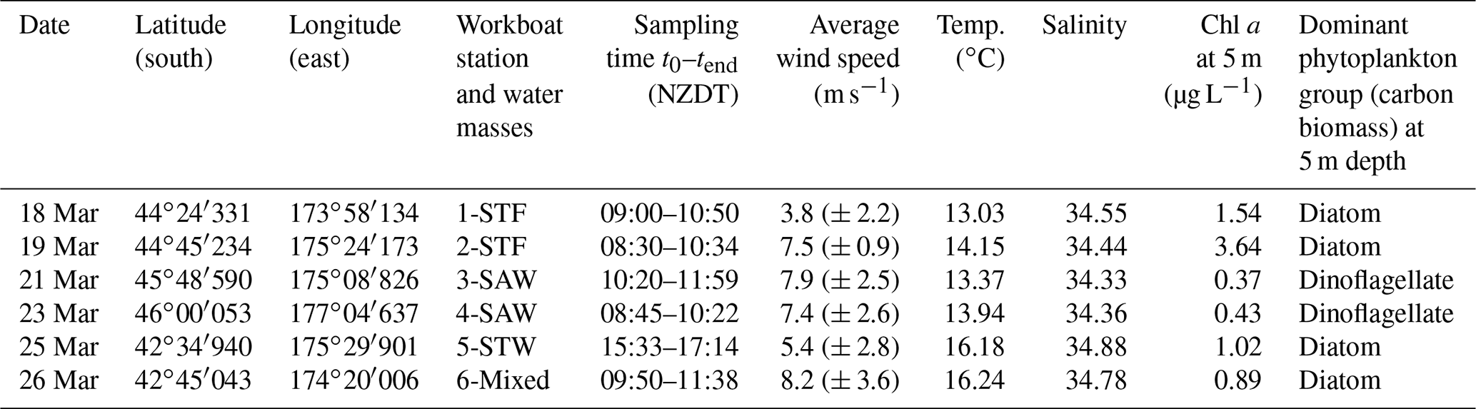
The Sea2Cloud voyage took place from 16 to 28 March 2020 (austral autumn) onboard R/V Tangaroa in the Chatham Rise region (Fig. 1a). The characteristics of the water masses sampled during this voyage and meteorological conditions are summarized in Table 1. Six workboat deployments were carried out to sample the SML and SSW in different water mass types: STF at stations 1 and 2, SAW at stations 3 and 4, and STW at station 5 (see Fig. 1a, Table 1). Mixed water (Mixed) at station 6 was a composite of coastal and shelf water from Cook Strait and STW, with higher nutrient content than STW, as presented in Fig. 1b. Local wind measurements were obtained from an automatic weather station (AWS) located at 25.2 m above sea level above the bridge of the R/V Tangaroa, which was exposed to all wind directions (Smith et al., 2018).

Figure 1(a) Sea2Cloud voyage track overlain by sea surface temperature (∘C) using Ocean Data View (Schlitzer, 2020), with workboat station positions and water mass type identified. The grey shading shows the seafloor topography, with the darker grey band along 43.5∘ S indicating the location of the Chatham Rise. (b) Nitrate concentration during the Sea2Cloud voyage, measured at 5 m. Water mass type is indicated by the labels at the top of the figure and separated by the grey vertical dashed lines.
Table 1Summary of environmental conditions during the workboat deployments. Waterside variables were determined from the vessel underway system, which sampled at 5 m depth; wind speed was measured by AWS and is presented as the average (± standard deviation) over the previous 12 h before sampling.
2.2 Sampling of the SML
The SML and SSW were sampled from a workboat 0.5 to 1 nmi (nautical miles) away from the R/V Tangaroa between 08:00 and 12:00 NZDT during periods when the wind speed was below 10 m s−1 (Table 1). Station 5-STW was an exception as it was sampled in the afternoon due to high wind speed in the morning (> 10 m s−1). Dissolved DMS in the SML was sampled using a novel gas-permeable tube technique in which a 280 cm long loop of silicone tube (external diameter 2.41 mm, wall thickness 0.49 mm) was deployed on the sea surface. The gas-permeable tube was filled with Milli-Q® water prior to deployment and closed by joining the two tube ends with a union. The gas-permeable tube was threaded through floating beads to ensure contact with the SML and deployed free-floating upstream of the workboat. Once in contact with the SML, the technique relies upon diffusion of DMS through the gas-permeable tube membrane across the concentration gradient between seawater and Milli-Q® water. In theory at least 50 % of the tube surface area is in contact with the SML and surface seawater, with the remainder exposed to the atmosphere. The gas-permeable tube was recovered after 10 min, with the Milli-Q® water withdrawn immediately using a syringe and stored in a chilly bin. SML sampling was carried out in duplicate at each station.
Prior to deployment in the field, the diffusion efficiency of the gas-permeable tube was determined in semi-controlled conditions using coastal seawater (Wellington, New Zealand) that was naturally elevated in DMS (range: 1.25–16.88 nmol L−1, average 4.94 nmol L−1). The calibration tank was continuously filled with seawater at a flow rate of 75 L min−1, with a constant overflow to ensure that there was no SML formation; this approach resulted in a uniform and homogenous DMS concentration in the tank for the gas-permeable tube to equilibrate with. The gas-permeable tube was filled with Milli-Q® water and placed on the surface of the seawater in the tank for 10 min, after which the Milli-Q® water was withdrawn into a syringe with no headspace whilst the gas-permeable tube remained in contact with the surface water. The 10 min exposure time was predetermined in laboratory experiments and represented the optimum time to achieve significant diffusion efficiency whilst reducing deployment time. The gas-permeable tube was then removed from the water and refilled with Milli-Q® water, and the experiment was repeated three to eight times. In addition, ambient seawater in the calibration tank was sampled at t0 and t+10 min for each repetition. Between each repetition, samples were transferred to the laboratory for immediate analysis. The DMS diffusion efficiency was subsequently determined using Eq. (1):
where [DMS]MQ is the DMS concentration measured in the Milli-Q® water at t+10 min, and [DMS]tank is the averaged DMS concentration between t0 and t+10 min measured in the calibration tank. The average D for 10 min exposure was 61 % (± 10 % standard deviation, n=19) as determined over a 4-month period during which the seawater temperature range was similar to that during the Sea2Cloud voyage at 12–16 ∘C. Further details of the gas-permeable tube technique are provided in Saint-Macary (2022). The average D was then applied to calculate the actual DMS concentration in the SML, [DMS]SML, using Eq. (2):
where [DMS]MQ is the DMS concentration in the Milli-Q® water after 10 min of exposure in the SML.
A glass plate (Harvey and Burzell, 1972) and a sipper were also used for sampling of DMSP, DMS, and ancillary variables in the SML. The sipper consists of a tube with multiple inlets that float on the sea surface. A syringe was used to slowly draw SML water through the open inlets to sample for chlorophyll a (Chl a), phytoplankton composition, and DMSP. The sipper external diameter was similar to the gas-permeable tube (2.2 and 2.4 mm, respectively), enabling sampling of a similar SML thickness but larger SML water volume. DMSP and DMS were also sampled with the plate for method comparison only. The repeatability for DMS sampling with the gas-permeable tube and plate was calculated using the standard deviation (Eq. 3, Olivieri and Faber, 2009) based upon two duplicates at each sampling event:
with σ the standard deviation, N the total number of terms, xi terms given in the data, and μ the mean.
2.3 Sampling of the SSW
For DMSP and DMS sampling of the SSW, a Teflon tube was deployed with the inlet at a depth of approximately 0.5 m by a system of ropes and fishing weights. 50 mL of SSW was withdrawn using a syringe and collected in an amber bottle, leaving no headspace. For larger volumes for other ancillary variables in the SSW, a bottle was immersed to 0.5 m below the surface and filled with seawater. To avoid SML contamination, the bottle was immersed with its lid on, then opened and closed in the SSW before recovery. For each variable the EF was calculated by dividing the concentration in the SML by its concentration in the SSW.
The conductivity–temperature–depth (CTD) sensor was launched between 10:00 and 12:15 following SML sampling, except at 5-STW when the CTD was deployed before the SML sampling at 07:00. Six depths from 5 to 150 m were sampled with 12 L Niskin bottles, although only the results from 5 m depth are discussed in this paper. For DMS sampling from the CTD casts, the water was overflowed by gravity by at least 100 % into amber bottles and then sealed with no headspace.
2.4 DMSP and DMS analytical system
For DMS measurements, water from the amber bottles was withdrawn in plastic Terumo® syringes. The samples were injected through a 25 mm glass microfiber filter (GF/F) into a 1 mL loop before transfer to a silanized sparging tower, where the sample was sparged for 5 min with nitrogen (N2) at a flow rate of 50 mL min−1. Nafion® dryers removed the water vapour from the gas stream before DMS preconcentration at −110 ∘C on a Tenax® trap. The trap was then heated to 120 ∘C to release the DMS onto an Agilent Technology 6850 gas chromatograph coupled to an Agilent 355 sulfur chemiluminescent detector (GC–SCD). The daily sensitivity and detection limit of the detector were confirmed using VICI® methyl ethyl sulfide and DMS permeation tubes. The average detection limit during the voyage was 0.14 (± 0.03) pgS s−1. For total DMSP measurements, 20 mL glass vials were filled with seawater and two pellets of sodium hydroxide added before gas-tight sealing of the vials, which were stored at ambient temperature in the dark. DMSP was analysed 1 d after sampling using the same semi-automated purge-and-trap system followed by GC–SCD, as described above. A wet standard calibration curve was made daily from a stock solution of DMSP diluted in Milli-Q® water, with calibration concentrations ranging from 0.1 to 95 nmol L−1. These were decanted into 20 mL gas-tight glass vials, hydrolyzed with two pellets of sodium hydroxide, and then injected into the sparging unit and processed as with the samples.
2.5 Ancillary variables
For Chl a analysis, 250 mL of seawater was filtered onto a 25 mm GF/F filter and then stored at −80 ∘C until analysis. Chl a was extracted in 90 % acetone, measured, and compared with Chl a standards using a Varian Cary Eclipse fluorometer with an accuracy of 0.5 nm at 541.2 nm. An acidification step was used to correct for pheophytin interference (10200 PLANKTON).
Phytoplankton community structure was determined for cells > 5 µm using a Flowcam (Fluid Imaging Technologies Inc). A sample of 250 mL of seawater was concentrated using a 47 mm diameter 3 µm polycarbonate filter to 10 mL final volume and stored at 4 ∘C until analysis. 1 mL of 25 times concentrated seawater sample was run through an 80 µm depth field-of-view flow cell (FC80FV) at 0.050 mL min−1 and 20 frames per second, with an imaging efficiency of 61.9 ± 2 %. Images were taken using a 10× objective on AutoImage mode. Total run time for each sample was 20 min. Between 4-SAW and 5-STW, the sample volume and flow rate were increased to 2 mL at 0.100 mL min−1, with an imaging efficiency of 32.7 %, due to the high abundance of large diatoms (e.g. Chaetoceros sp.). Images were classified into cell size and class groupings using VisualSpreadsheet v4.16.7 software by size category (< 10; 10 to 20; 20 to 50 and > 50 µm), and the results are given as total phytoplankton biovolume of each size class.
For microscopic analysis of phytoplankton community composition, 500 mL of seawater was preserved at 1 % (final concentration) Lugol's iodine solution, with samples stored at room temperature in the dark. Phytoplankton community composition and cell numbers for phytoplankton > 5 µm were determined using optical microscopy following the method described in Safi et al. (2007) and references herein. Briefly, 100 mL subsamples were settled for 24 h and the supernatant then carefully syphoned with 10 mL transferred to Utermohl chambers and resettled (Edler and Elbrächter, 2010). Where possible, all abundant organisms were identified to genus or species level before being counted. Phytoplankton biovolume estimates were calculated from the dimensions of each taxa and approximated geometric shapes (spheres, cones, ellipsoids) initially following Olenina et al. (2006). The biovolumes were subsequently used to calculate cell carbon (mg C m−3) using equations from the literature: Olenina et al. (2006) and Montagnes and Franklin (2001) for diatoms and Olenina et al. (2006) and Menden-Deuer and Lessard (2000) for dinoflagellates and nanoflagellates. Menden-Deuer and Lessard (2000) was also applied to other low-biomass unidentified groups referred to as small flagellates.
2.6 DMS air–sea flux calculation
The DMS air–sea flux, F, was calculated using the gas transfer flux equation (Liss and Merlivat, 1986) following Eq. (4):
with H the Henry's law solubility coefficient for DMS (Dacey et al., 1984), [DMS]w the dissolved DMS concentration, [DMS]atm the DMS concentration in the atmosphere, and kDMS, COARE the gas transfer coefficient. The latter was calculated using the NOAA COARE gas transfer (COAREG) version 3.6 algorithm (Fairall et al., 2003; Fairall et al., 2011) and parameterized in terms of local wind speed scaled to 10 m height, as described in Bell et al. (2015). The gas transfer velocity was adapted for DMS using the Schmidt number (Sc) calculated using local temperature (T) in degrees Celsius (∘C) (Saltzman et al., 1993) measured from the underway system at 5 m depth following Eq. (5).
The atmospheric DMS concentration [DMS]atm was neglected as this is several orders of magnitude lower than the dissolved DMS concentration (Kremser et al., 2021). Flux estimates were obtained using DMS concentrations from three different depths: FSML corresponds to DMS air–sea flux calculated using SML DMS concentration obtained with the gas-permeable tube, FSSW to DMS concentration in the SSW, and F5 m to DMS concentration at 5 m depth from the CTD.
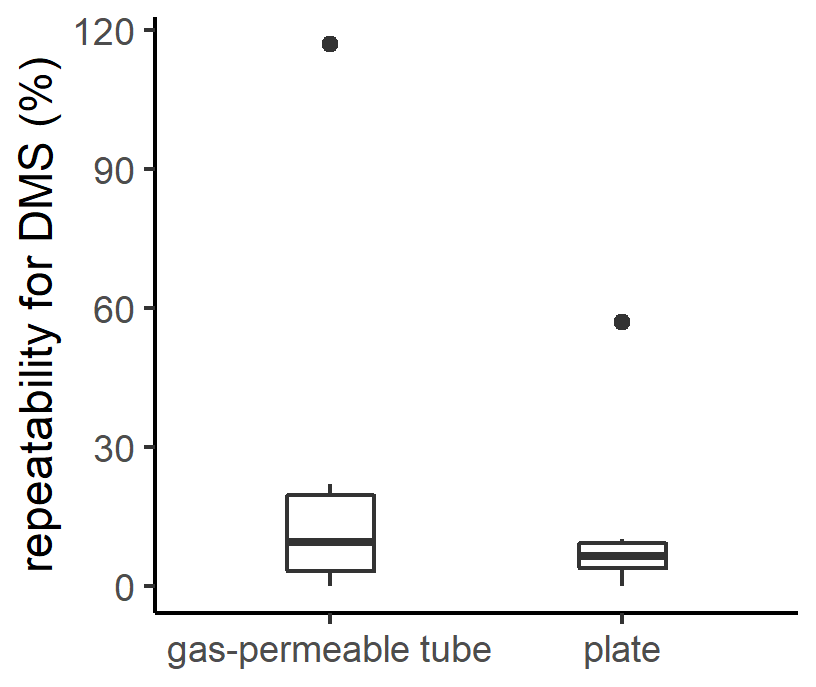
Figure 2Box plot of the repeatability for DMS measurements with the gas-permeable tube and the plate. The box plot represents the distribution of the data, with the box corresponding to the interquartile range and the bold horizontal line the median. The limits of the vertical lines represent the upper and lower fences. The outliers are represented by points outside the fences.
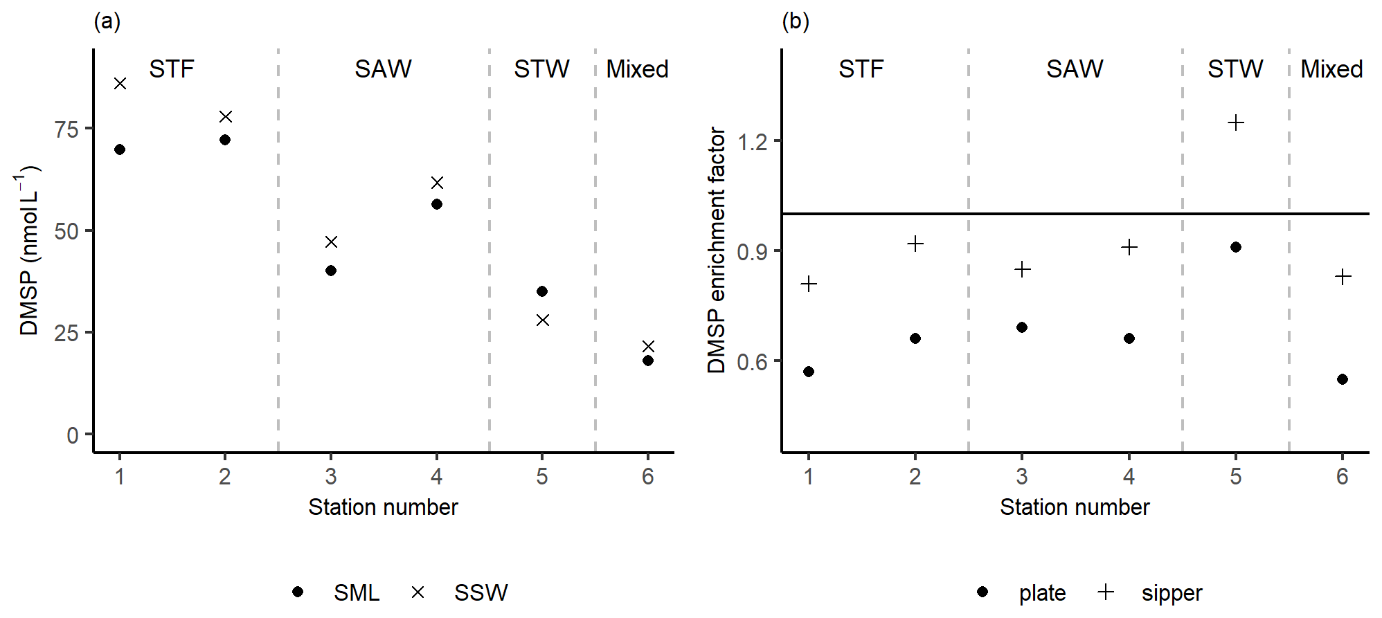
Figure 3(a) DMSP concentrations sampled in the sea surface microlayer (SML) by the sipper and in the subsurface water (SSW) and the (b) DMSP enrichment factor from the sipper and plate. Water mass type is indicated by the labels at the top of the figure and separated by the grey vertical dashed lines.
2.7 Statistical analysis
The Shapiro test was used to verify the normality of variable distribution. For the non-normally distributed variables Spearman's rank correlation was carried out, and for the normally distributed data a Pearson test was applied. Linear correlation was considered significant when the coefficient of correlation (rho and r for Spearman's rank and Pearson tests, respectively) was higher than 0.5 and p value was lower than 0.05.
3.1 Comparison of plate and gas-permeable tube
The repeatability of SML sampling techniques is generally not reported, although this is critical, particularly as the width and presence of the SML are inherently patchy and heterogenous (Frew et al., 2002; Ribas-Ribas et al., 2017). The repeatability of the plate and gas-permeable tube for DMS were similar although the plate had a smaller interquartile range (plate median 6 %; interquartile range 6 %, n=6; gas-permeable tube median 10 %; interquartile range 17 %, n=6; Fig. 2). The repeatability determined for DMS using the gas-permeable tube was subsequently applied in the current study to identify a significance threshold, with no significant difference between SML and SSW DMS assigned where EF was within 0.90–1.10.
3.2 DMSP and DMS in the SML and SSW
The DMSP concentration was highest in the SML and SSW of STF, with an average of 76 nmol L−1 (Fig. 3a), and lowest in STW and Mixed water at 32 and 20 nmol L−1, respectively. The average EF DMSP was 0.93 (range: 0.81–1.25) with enrichment only observed at 5-STW (Fig. 3b). Sampling with the plate showed a spatial trend similar to the sipper, but with lower average EF DMSP of 0.67 (range: 0.55–0.91) and no enrichment of DMSP at any station. The higher DMSP concentrations with the sipper may reflect the fact that this method samples some water from immediately below the SML, whereas the plate only withdraws the organic layer associated with the SML (Harvey and Burzell, 1972; Cunliffe and Wurl, 2014).
Three stations, 3-SAW, 5-STW, and 6-Mixed, had relatively low DMS concentrations of ∼ 1.5 nmol L−1 with no significant difference in concentration between the SML, SSW, and 5 m depth (Fig. 4a). In contrast, the DMS concentration in the SSW was generally higher at the other three stations, ranging from 4.2 to 6.4 nmol L−1, whilst concentrations in the SML and at 5 m were similar, indicating an SSW maximum in DMS. The gas-permeable tube showed no DMS enrichment at five of the six stations, with only 3-SAW showing significant SML enrichment. The overall average EF DMS was 0.83 (range: 0.40–1.22), with three stations showing DMS depletion in the SML. Conversely, when the plate was used to sample the SML significant depletion in DMS was apparent at all stations, with an average EF DMS of 0.46 (range: 0.28–0.68; Fig. 4b), suggesting loss of DMS by sampling with the plate.
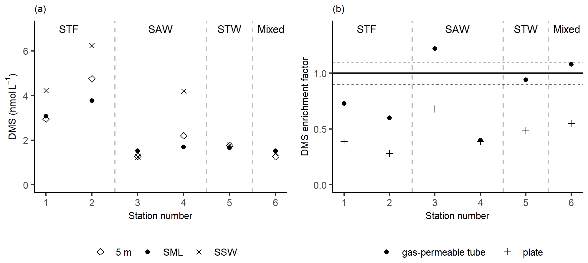
Figure 4(a) DMS concentrations in the sea surface microlayer (SML) (using the gas-permeable tube), subsurface water (SSW), and at 5 m depth. (b) DMS enrichment factor determined by the gas-permeable tube and glass plate. The horizontal dashed lines represent the significance threshold determined from the median repeatability of the gas-permeable tube (10 %). Water mass type is indicated by the label at the top of the figure and separated by the grey vertical dashed lines.
3.3 Ancillary variables
3.3.1 Chl a
The highest Chl a concentrations (∼ 4.3 µg L−1) were found at 2-STF in the SML and SSW, with lower uniform Chl a concentrations (average 0.5 µg L−1) at the two surface depths at 3-SAW, 4-SAW, and 6-Mixed (Fig. 5a). Average EF Chl a was 0.91 (range: 0.50–1.06), with enrichment in the SML at 1-STF, 3-SAW, and 4-SAW (Fig. 5b).
3.3.2 Phytoplankton community
Phytoplankton abundance, as determined using the Flowcam, is described in terms of total biovolume (> 5 µm) and also for the separate size fractions (< 10, 10–20, 20–50, and > 50 µm) (Fig. 6). Total phytoplankton biovolume was highest at 2-STF (8.55×10⁸ to 1.13×109 µm3 L−1) and lowest at 3-SAW and 6-Mixed (2.93×10⁷ to 8.16×107 µm3 L−1). Station 1-STF displayed high biovolume in the SML but low biovolume in SSW (2.90×10⁸ and 4.80×107 µm3 L−1, respectively). Differences in dominant phytoplankton size fraction were apparent between stations. The 10–20 µm fraction was dominant at 2-STF (62 % and 54 % in the SML and SSW, respectively) and 4-SAW (85 % in the SML and SSW), whereas the 20–50 µm fraction dominated at station 5-STW (42 % and 49 % in the SML and SSW, respectively) and in the SML at 1-STF (43 %), but it was lowest in the SML at 3-SAW (15 %). The < 10 µm size fraction generally accounted for the smallest biovolume (< 10 %), except in the SML at 6-Mixed where it was the dominant size fraction (30 %). Variations were generally consistent within stations, with similar size fraction abundance in the SML and SSW, except at 1-STF, which showed a lower biovolume in the > 50 µm fraction and corresponding higher biovolume in the 10–20 µm fraction in the SML.
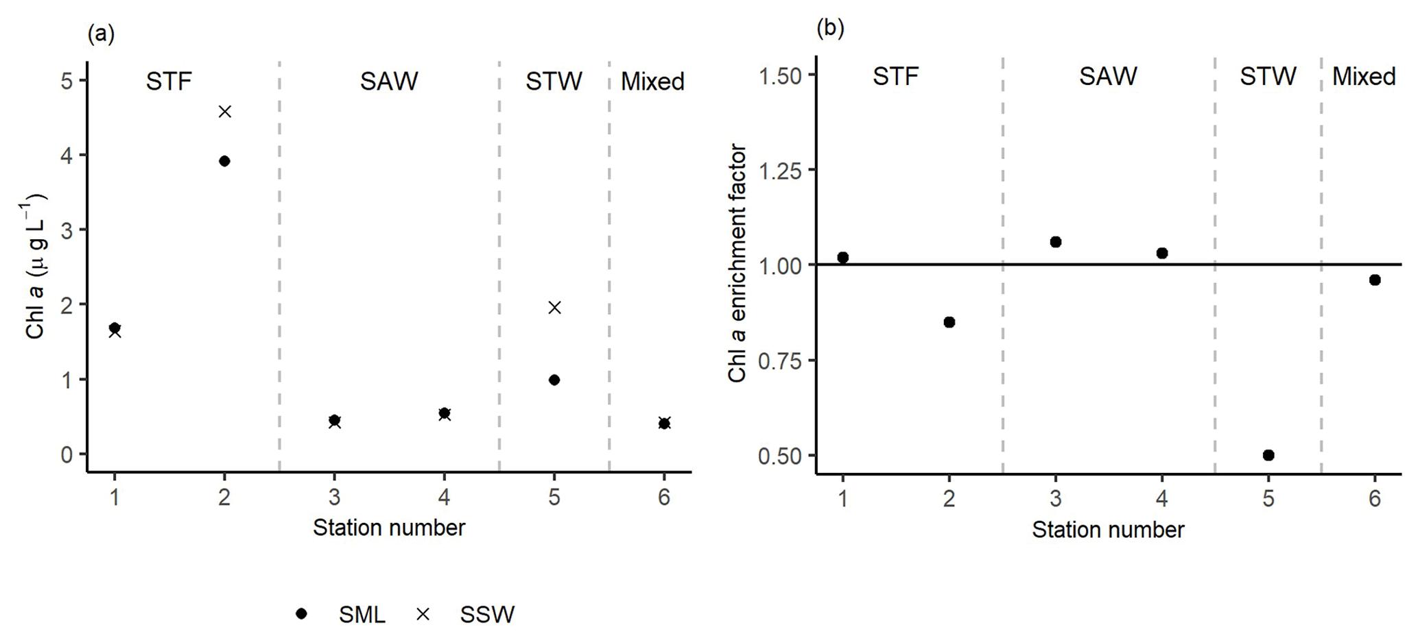
Figure 5(a) Chl a concentrations in the sea surface microlayer (SML) and subsurface water (SSW), as well as the (b) Chl a enrichment factor. Water mass type is indicated by the label at the top of the figure and separated by the grey vertical dashed lines.
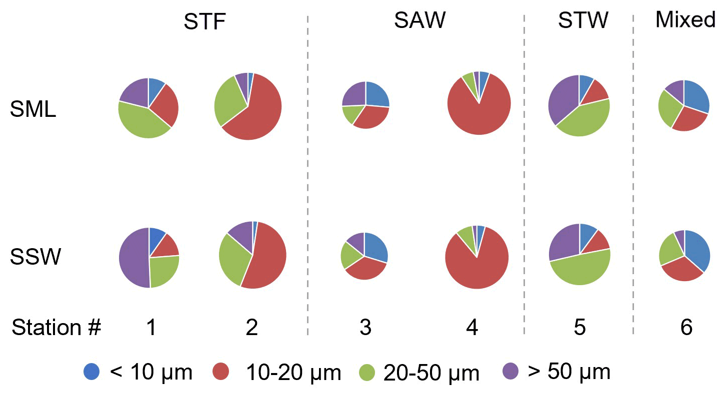
Figure 6Pie charts showing the relative variation of phytoplankton size fraction in the sea surface microlayer (SML) and subsurface water (SSW) at the six stations. The size of the pie is proportional to the total summed biovolume (in µm3 L−1) for phytoplankton > 5 µm, with the coloured wedges corresponding to the different size fractions. Water mass type is indicated by the label at the top of the figure and separated by the grey vertical dashed lines.
The composition of the phytoplankton community was also examined in terms of carbon biomass (Fig. 7). Total phytoplankton biomass was highest at 1-STF and in SSW at 2-STF and 5-STW (22 to 31 mg C m−3), and it was lowest at 3-SAW and 6-Mixed (3.9 to 8.3 mg C m−3). The phytoplankton groups in the SML and SSW varied with water mass, with dinoflagellates dominating at all stations, except 2-STF and 5-STW where diatoms dominated (2-STF SSW 52 %; 5-STW SML 75 %, SSW 61 %). Dinoflagellate biomass in the SML and SSW averaged 7.4 mg C m−3, with a maximum at 1-STF (18 mg C m−3) and minimum at 5-STW (1.6 mg C m−3, Supplement Fig. S1), whereas diatom biomass was generally lower with a maximum at 5-STW (19 mg C m−3) and minimum at 3-SAW (0.1 mg C m−3, Supplement Fig. S1). The small flagellates had lower biomass (< 16 %), except at 3-SAW and 6-Mixed (SML 28 % and 43 %, respectively, and SSW 9 % and 37 %, respectively). The dominant phytoplankton genus (> 5 µm) was the dinoflagellate Gymnodinium, which accounted for more than 10 % of total phytoplankton biomass in the SML at 1-STF, 3-SAW, and 4-SAW and 6 % at 6-Mixed (Supplement Fig. S2).
There was no difference in dominant phytoplankton group between the SML and SSW at all stations. There was generally lower dinoflagellate biomass in the SML relative to the SSW (Fig. 8), with an average EF of 0.75 (range: 0.19–1.43) with enrichment only observed at 1-STF (1.43) and 4-SAW (1.14). Diatom biomass was also lower in the SML, with an average EF of 0.62 (range: 0.31–1.09) and only 1-STF showing enrichment (1.09).
3.4 Correlations between variables
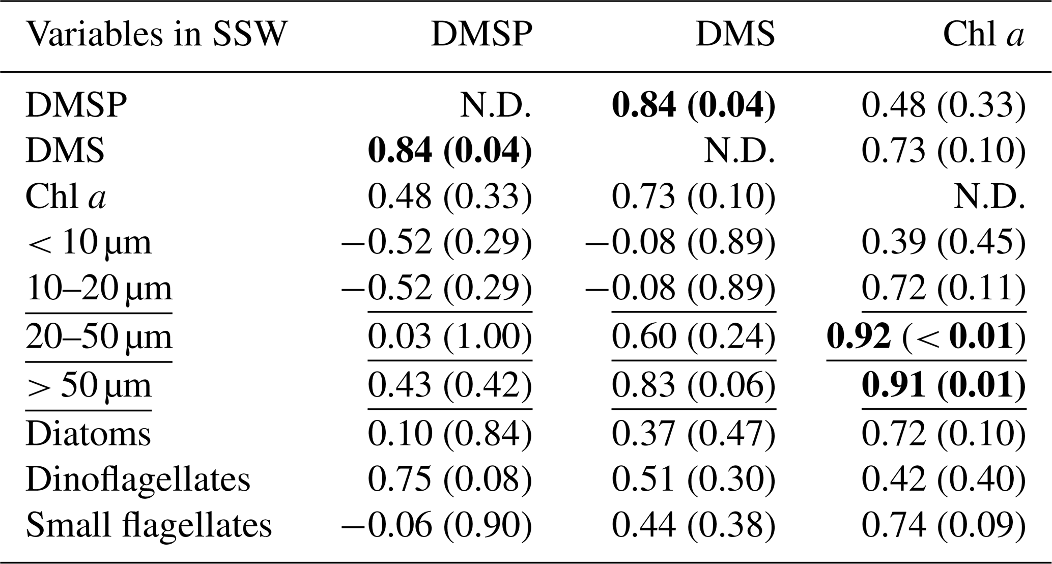
At all stations the Pearson test identified DMSP concentration and diatom biomass in the SML as significantly correlated with their respective concentrations in the SSW (r=0.95, p < 0.01 for DMSP and r=0.92, p= 0.03 for diatoms). The SML DMS concentration presented in this section was obtained from the gas-permeable tube and was not normally distributed. In addition, DMSP and DMS were correlated in both the SML and SSW (Spearman's rank test for the SML and Pearson test for the SSW; Tables 2 and 3). The DMSP concentration was also correlated with dinoflagellate biomass in the SML (Pearson test, Table 2). The Spearman's rank test established that Chl a and DMS in the SML correlated with their respective concentrations in the SSW (rho = 0.99, p < 0.01 for DMS and rho = 0.94, p=0.02 for Chl a), and DMS concentration in the SML also correlated with SML Chl a concentration, the 20–50 µm fraction (Spearman's rank test; Table 2), and the biomass of the dinoflagellate Gymnodinium (rho = 0.95; p=0.05; Spearman's rank test; Supplement). In the SSW, 20–50 and > 50 µm size fractions correlated with the Chl a concentration (Table 3). The correlations were all positive.
Table 2Summary of Pearson test and Spearman's rank correlation (underlined) for DMSP, DMS, and all ancillary variables in the SML. The correlations are significant where r or rho (for Pearson and Spearman's rank tests, respectively) is > 0.5 and p < 0.05, as indicated in bold. The size fraction biovolumes were obtained from Flowcam, and the phytoplankton community composition was obtained from optical microscopy. N.D. stands for no data. SML DMS was sampled with the gas-permeable tube.

Table 3Summary of Pearson test and Spearman's rank correlation (underlined) for DMSP, DMS, and all ancillary variables in the SSW. The correlations are significant where r or rho (for Pearson and Spearman's rank tests, respectively) is > 0.5 and p < 0.05, as indicated in bold. The size fraction biovolumes were obtained from Flowcam, and the phytoplankton community composition was obtained from optical microscopy. N.D. stands for no data.
3.5 Air–sea flux
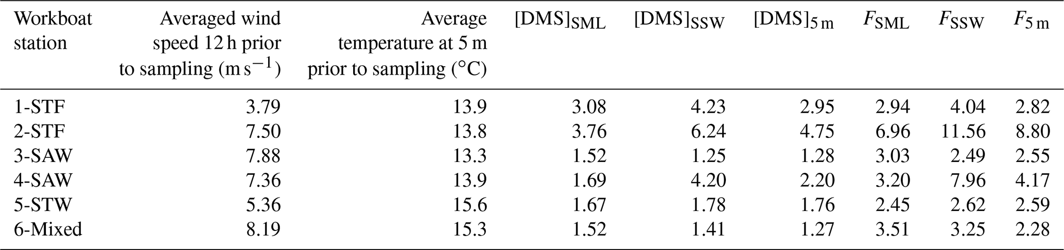
Average wind speeds over the previous 12 h ranged from 3.79 to 8.19 m s−1 for the workboat sampling. The air–sea flux was calculated over the 12 h prior to sampling the SML as the SML structure and near-surface mixing would be influenced by winds over a longer preceding period than instantaneous winds. Average DMS fluxes were 3.68 µmol m−2 d−1 (range: 2.45–6.96 µmol m−2 d−1) for FSML and 5.32 µmol m−2 d−1 (range: 2.49–11.56 µmol m−2 d−1), with generally higher DMS fluxes recorded at higher wind speeds combined with higher DMS concentrations as expected (Table 4). Air–sea flux was also calculated using DMS concentration at 5 m depth (F5 m) and compared with the SML and SSW fluxes to examine the influence of depth on calculated flux. Although FSML and F5 m exhibited differences across workboat stations, the average F5 m of 3.87 µmol m−2 d−1 (range: 2.28–8.80 µmol m−2 d−1) was consistent with the average FSML. The difference in DMS air–sea flux calculated for the three different depths was primarily due to the higher DMS concentration in the SSW.
Table 4DMS air–sea flux calculated using the COARE algorithm for each station. SML DMS concentration was obtained with the gas-permeable tube. DMS concentrations are in nmol L−1, and the flux is expressed in µmol m−2 d−1.
From a regional perspective, the Sea2Cloud results contrast with previous studies (Law et al., 2017; Walker et al., 2016), with lower DMS concentrations encountered in SSW and SML DMS enrichment at only one of the six stations. Furthermore, Chl a enrichments in the SML were low, contrary to that reported in other studies (Yang et al., 2009; Zhang et al., 2008, 2009). Enrichment of biogeochemical variables, such as Chl a, DMSP, and DMS, in the SML has often been observed during a phytoplankton bloom in the underlying water (Nguyen et al., 1978; Yang et al., 2005a; Zhang et al., 2009; Walker et al., 2016); however, the diatom bloom of 4.3 µg L−1 Chl a at 2-STF exceeded the maximum Chl a concentrations recorded during the previous SOAP voyage (2.8 µg L−1; Lizotte et al., 2017) and was insufficient to generate Chl a, DMS, or DMSP enrichments in the SML. These contrasting regional results (Bell et al., 2015; Walker et al., 2016; Lizotte et al., 2017) suggest nonoptimal conditions for DMS and Chl a enrichment in the SML in the current study.
SML DMSP concentration was primarily influenced by dinoflagellate biomass, as indicated by the positive correlation between these variables (Table 2). This is consistent with previous observations, in which DMSP enrichment in the SML was attributed to phytoplankton composition (Yang and Tsunogai, 2005; Zemmelink et al., 2006), particularly when dinoflagellates were dominant (Yang, 1999; Matrai et al., 2008; Yang et al., 2009). However, DMSP was not enriched in the SML during the SOAP voyage, despite the high dinoflagellate biomass (Cliff Law, personal communication, 2022), and SML enrichment only occurred at one station in the current study where the ratio of dinoflagellate to diatoms was the lowest (5-STW, 0.2, Fig. 3b). The correlation between DMSP and dinoflagellates was high in both SML and SSW in the current study but only significant in the SML, indicating that specific factors enhance this relationship in the SML. DMSP production increases under oxidative stress (Sunda et al., 2002), so light stress may be a co-factor that enhances DMSP production by dinoflagellates in the SML.
The complexity of DMS cycling often precludes identification of the main drivers of DMS production, and this is particularly so in the SML where loss of DMS to the atmosphere obscures potential relationships with conservative properties such as Chl a and phytoplankton group (Stefels et al., 2007; Bürgermeister et al., 1990; Townsend and Keller, 1996; Turner et al., 1988). Indeed, only one study has previously reported a correlation between enrichment of Chl a and DMS in the SML (Yang and Tsunogai, 2005). However, DMS concentration in the SML was correlated with both the Chl a and 20–50 µm size fraction in the current study (Table 2). During SOAP, high DMS EF and concentrations were associated with a dinoflagellate bloom (Walker et al., 2016), with Gymnodinium and Gyrodinium being the most abundant genera, in addition to Ceratium and small flagellates (Cliff Law, personal communication, 2022, Supplement Fig. S3). In both SOAP and the current study, SML DMS was significantly correlated with Gymnodinium (Spearman's rank test; rho = 0.95, p= 0.05 and rho = 0.76, p= 0.02, respectively). The relationship between DMS and dinoflagellates is consistent with dinoflagellates being a source of DMSP, but DMSP conversion to DMS may also potentially be enhanced by other factors. For example, copepod grazing on Gymnodinium is reported to influence DMS concentration (Dacey and Wakeham, 1986). Moreover, during senescence, dinoflagellates release gel-like compounds that accumulate in the SML (Jenkinson et al., 2018), altering the physical properties of the SML and influencing gas exchange (Wurl et al., 2016). Consequently, dinoflagellates affect DMSP and DMS both directly and indirectly in the SML.
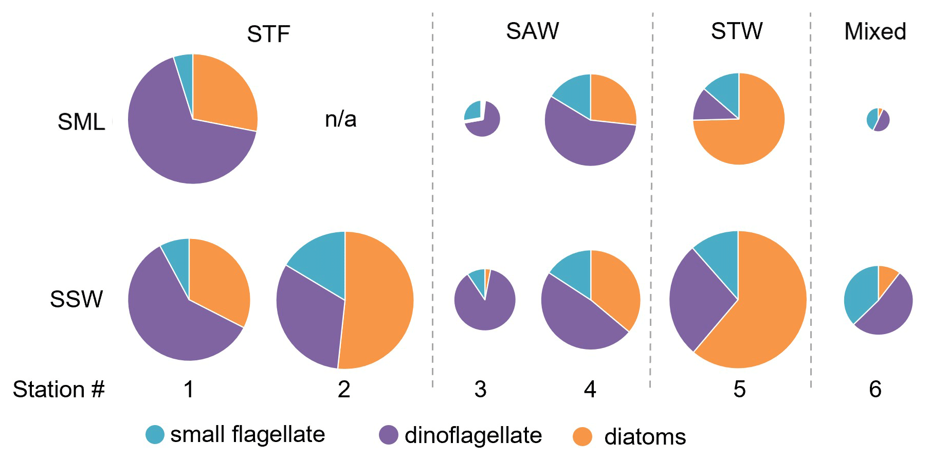
Figure 7Pie charts showing the relative variation of diatoms, dinoflagellate, and small flagellates in the sea surface microlayer (SML) and subsurface water (SSW). The size of the pie is proportional to the total carbon content of phytoplankton > 5 µm. Water mass type is indicated by the label at the top of the figure and separated by the grey vertical dashed lines. There are no data for SML 2-STF as the sample was not obtained.
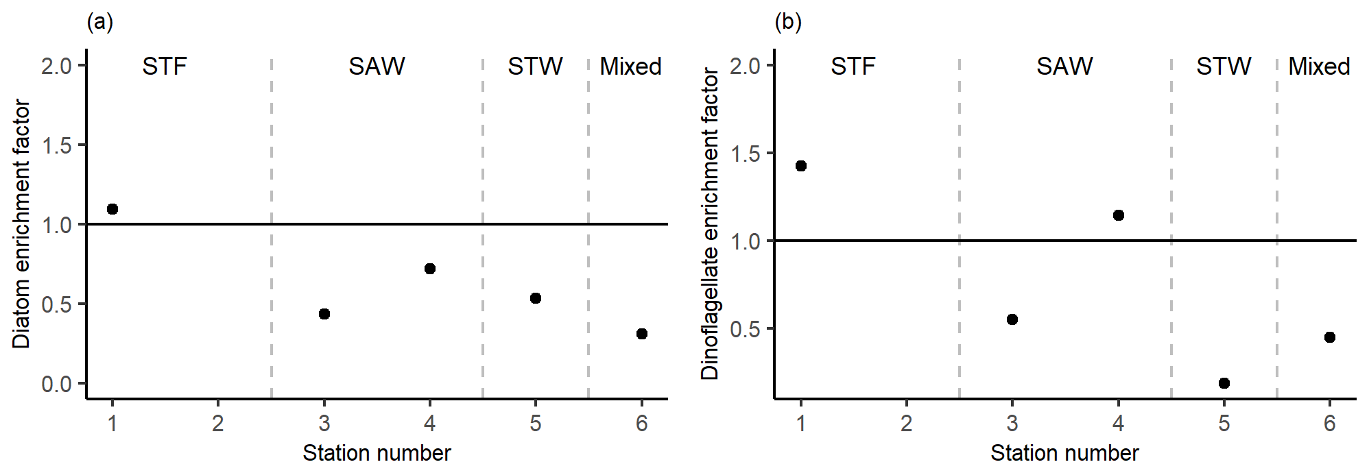
Figure 8Phytoplankton carbon content enrichment factors for (a) diatoms and (b) dinoflagellates > 5 µm. Water mass type is indicated by the label at the top of the figure and separated by the grey vertical dashed lines.
DMS loss is expected to be more rapid in the SML due to its proximity to the atmosphere. However, other processes such as elevated photo-oxidation of DMS in the SML may also contribute to DMS removal in the surface ocean (Saint-Macary et al., 2022). The DMS maximum in the SSW relative to the SML and 5 m depth (Fig. 4a) may reflect a combination of near-surface stratification and elevated DMS ventilation at the surface. This is in contrast to the observations of Walker et al. (2016) in the same region, who reported the opposite effect, with high DMS enrichment in the SML. The latter may have arisen from an optimal combination of factors: (i) a dinoflagellate bloom supporting elevated DMSP and resulting DMS production (Walker et al., 2016) and (ii) favourable meteorological conditions, i.e. very low wind speeds (Law et al., 2017), that limited near-surface mixing and led to (iii) near-surface stratification (Smith et al., 2018). Although near-surface temperature measurements were not obtained during the current study, wind speeds were generally higher than during SOAP, indicating higher mixing and reduced potential for near-surface stratification, although the sole observation of DMS enrichment occurred at the station with the highest wind speeds (see Table 4). Contrasting near-surface DMS gradients have been reported in a stratified salt pond (Zemmelink et al., 2006) and coastal water under calm meteorological conditions (Zemmelink et al., 2005), with respective increases and decreases in DMS concentration to the surface. The key factor determining DMS enrichment or depletion in the SML in these studies was irradiance, which stimulated DMSP production via the phytoplankton antioxidant response in the salt pond (Zemmelink et al., 2006), and DMS photo-oxidation in the stratified coastal water (Zemmelink et al., 2005). Consequently, consideration of the physical controls in addition to biogeochemical processes is required to explain DMS enrichment in the SML (assessed in a companion paper; Saint-Macary et al., 2022). An additional factor influencing enrichment may be the presence of surfactant, which can act as a barrier to gas transfer (Broecker et al., 1978; Goldman et al., 1988; Pereira et al., 2016). Surfactant, measured in mg L−1 TX-100 equivalents (Sigma Aldrich, TritonX 100), was enriched at half of the stations (3-SAW, 4-SAW, and 6-Mixed; Theresa Barthelmeß, personal communication, 2022), one of which showed DMS enrichment in the SML, although there was no correlation between surfactant and DMS in terms of concentration or enrichment.
The current study also highlighted variation in the sampling efficiency of different methodological approaches for determining DMS enrichment in the SML. The higher DMS concentrations obtained with the gas-permeable tube relative to the glass plate may reflect the fact that the water sample in the gas-permeable tube is less exposed to air during the sampling procedure than with techniques such as the plate, screen, and rotating drum (Yang, 1999; Zhang et al., 2009; Matrai et al., 2008; Zemmelink et al., 2006). Loss to the atmosphere is generally not accounted for in other SML studies (Zemmelink et al., 2005; Yang et al., 2001). DMS is potentially lost with the gas-permeable tube, as the upper surface is exposed to the atmosphere; however, this is minimized by smearing of the SML over the tube by surface turbulence, and gas loss is also accounted for by the diffusion efficiency correction (see the Method section). When sampled with the plate and the screen the EF DMS was shown to be affected by environmental conditions and sampling thickness (Yang et al., 2001). As the plate samples a thinner layer than the gas-permeable tube (nominally 20–150 µm – Cunliffe et al., 2013 – and 1.21 mm, respectively), this may also result in a lower DMS concentration, depending on the SSW concentration. However, the plate samples the organics and bacteria of the SML, which may induce in vitro reactions in the sample bottle prior to analysis that may affect DMS concentration, whereas these are excluded with the gas-permeable tube. Another advantage of the gas-permeable tube is that it eliminates exposure of the water sample to high light, as with the plate and screen, thereby avoiding stress-induced responses and cell lysis. Patchiness of the SML (Frew et al., 2002; Ribas-Ribas et al., 2017) is an issue that will decrease the repeatability of all SML sampling techniques, but the larger surface coverage of the gas-permeable tube may decrease this variability. Yet, despite the increased effectiveness of the permeable tube technique for dissolved gases, the results indicate that DMS is not significantly enriched in the SML, in contrast to other studies that have used the plate and screen (Nguyen et al., 1978; Yang, 1999; Yang and Tsunogai, 2005; Yang et al., 2001, 2005a; Zhang et al., 2009; Walker et al., 2016; Zemmelink et al., 2006). Excluding the methodological shortcomings detailed here, this anomaly may reflect differing environmental conditions between studies; however, environmental conditions are rarely reported, and only a few have considered DMS fate in the SML (Zemmelink et al., 2005, 2006; Matrai et al., 2008; Walker et al., 2016). Consequently, it is difficult to draw conclusions as to whether previously reported DMS enrichments are artefacts, which limits the identification of the factors responsible for DMS enrichment.
DMS air–sea flux was calculated using the COARE algorithm, which was originally developed and tested based upon a representative depth of 5 m for surface waters (Huebert et al., 2004); consequently, this approach may be less appropriate for application to the SML where conditions are not as homogenous as water at 5 m (Frew et al., 2002; Ribas-Ribas et al., 2017). Regardless, the calculated fluxes based upon three different depths were consistent and also low relative to previous regional measurements during the SOAP campaign, in which DMS flux reached 100 µmol m−2 d−1 (Bell et al., 2015; Walker et al., 2016). The large difference in flux between SOAP and the regional climatological estimate Lana et al. (2011) primarily reflects the high DMS concentration in the dinoflagellate bloom during SOAP, whereas the lower DMS concentrations and emission during the current study reflect differing phytoplankton community composition, surface ocean dynamics, and also potentially different process rates (Saint-Macary et al., 2022).
The current study presents the first application of a robust sampling technique for trace gases in the SML that identified higher DMS concentrations relative to the standard SML sampling technique of the plate (Fig. 4b). However, DMSP and DMS were generally not enriched in the SML, with significant enrichment of both species observed at only one of six stations and low Chl a enrichment despite sampling of different water masses, phytoplankton biomass, and community composition. However, relationships were apparent between DMSP, DMS, dinoflagellate biomass, and the genus Gymnodinium biomass, suggesting that SML DMS and DMSP production may be enhanced in the presence of dinoflagellates. These observations complement the results from a previous study in the same region indicating that an optimal combination of physical and biological conditions is required for DMS enrichment in the SML. The calculated DMS air–sea fluxes were consistent with regional estimates in the Lana et al. (2011) and Wang et al. (2020) climatology models and indicate that DMSP and DMS cycling in the SML does not significantly influence regional air–sea DMS flux. These results raise questions regarding the significance of DMS enrichment in the SML and also how this can be maintained at the ocean interface where loss to the air dominates. Therefore, these results emphasize the need for DMS process studies in the SML (Saint-Macary et al., 2022).
Flux calculation code is available upon request.
For data availability please contact cliff.law@niwa.co.nz.
The supplement related to this article is available online at: https://doi.org/10.5194/os-19-1-2023-supplement.
ADSM, TB, and CSL developed the sampling strategy and collected the samples. ADSM wrote the paper and analysed DMSP and DMS. AM contributed to DMSP and DMS analysis. SD analysed samples on the Flowcam and processed results, and KS identified the species by optical microscopy. Nutrient and Chl a data were collected by KS and SD. RCS and MH calculated the DMS air–sea flux. ADSM interpreted the results, with guidance from CSL.
The contact author has declared that none of the authors has any competing interests.
Publisher's note: Copernicus Publications remains neutral with regard to jurisdictional claims in published maps and institutional affiliations.
This article is part of the special issue “Sea2Cloud (ACP/OS inter-journal SI)”. It is not associated with a conference.
We would like to thank Antonia Cristi and Wayne Dillon for their help during the Sea2Cloud campaign and Karen Thompson for flow cytometry analysis. We would also like to thank the officers and crew of the R/V Tangaroa for their support and expertise.
This research has been supported by NIWA SSIF funding to the Ocean–Climate Interactions Programme. Alexia D. Saint-Macary's PhD was funded by a University of Otago Departmental Award.
This paper was edited by Mario Hoppema and reviewed by two anonymous referees.
Bell, T. G., De Bruyn, W., Marandino, C. A., Miller, S. D., Law, C. S., Smith, M. J., and Saltzman, E. S.: Dimethylsulfide gas transfer coefficients from algal blooms in the Southern Ocean, Atmos. Chem. Phys., 15, 1783–1794, https://doi.org/10.5194/acp-15-1783-2015, 2015.
Boyd, P., LaRoche, J., Gall, M., Frew, R., and McKay, R. M. L.: Role of iron, light, and silicate in controlling algal biomass in subantarctic waters SE of New Zealand, J. Geophys. Res.-Ocean., 104, 13395–13408, https://doi.org/10.1029/1999JC900009, 1999.
Broecker, H. C., Petermann, J., and Siems, W.: The influence of wind on CO2-exchange in a wind-wave tunnel, including the effects of monolayers, J. Mar. Res., 36, 595–610, 1978.
Bürgermeister, S., Zimmermann, R., Georgii, H. W., Bingemer, H., Kirst, G., Janssen, M., and Ernst, W.: On the biogenic origin of dimethylsulfide: relation between chlorophyll, ATP, organismic DMSP, phytoplankton species, and DMS distribution in Atlantic surface water and atmosphere, J. Geophys. Res.-Atmos., 95, 20607–20615, https://doi.org/10.1029/JD095iD12p20607, 1990.
Carpenter, L. J. and Nightingale, P. D.: Chemistry and release of gases from the surface ocean, Chem. Rev., 115, 4015–4034, https://doi.org/10.1021/cr5007123, 2015.
Charlson, R. J., Lovelock, J. E., Andreae, M. O., and Warren, S. G.: Oceanic phytoplankton, atmospheric sulphur, cloud albedo and climate, Nature, 326, 655–661, 1987.
Chiswell, S. M., Bostock, H. C., Sutton, P. J., and Williams, M. J.: Physical oceanography of the deep seas around New Zealand: a review, New Zeal. J. Mar. Fresh., 49, 286–317, https://doi.org/10.1080/00288330.2014.992918, 2015.
Cunliffe, M. and Wurl, O.: Guide to best practices to study the ocean's surface, Occasional Publications of the Marine Biological Association of the United Kingdom (Plymouth, UK), 118, http://plymsea.ac.uk/6523/ (last access: 19 December 2022), 2014.
Cunliffe, M., Engel, A., Frka, S., Gašparoviæ, B., Guitart, C., Murrell, J. C., Salter, M., Stolle, C., Upstill-Goddard, R., and Wurl, O.: Sea surface microlayers: A unified physicochemical and biological perspective of the air–ocean interface, Prog. Oceanogr., 109, 104–116, https://doi.org/10.1016/j.pocean.2012.08.004, 2013.
Curson, A. R., Liu, J., Martínez, A. B., Green, R. T., Chan, Y., Carrión, O., Williams, B. T., Zhang, S.-H., Yang, G.-P., and Page, P. C. B.: Dimethylsulfoniopropionate biosynthesis in marine bacteria and identification of the key gene in this process, Nat. Microbiol., 2, 17009, https://doi.org/10.1038/nmicrobiol.2017.9, 2017.
Dacey, J. W. and Wakeham, S. G.: Oceanic dimethylsulfide: production during zooplankton grazing on phytoplankton, Science, 233, 1314–1316, https://doi.org/10.1126/science.233.4770.1314, 1986.
Dacey, J. W., Wakeham, S. G., and Howes, B. L.: Henry's law constants for dimethylsulfide in freshwater and seawater, Geophys. Res. Lett., 11, 991–994, https://doi.org/10.1029/GL011i010p00991, 1984.
Edler, L. and Elbrächter, M.: The Utermöhl method for quantitative phytoplankton analysis, Microscopic and molecular methods for quantitative phytoplankton analysis, edited by: Karlson, B., Cusack, C., and Bresnan, E., UNESCO, Paris, 13–20, 2010.
Fairall, C., Yang, M., Bariteau, L., Edson, J., Helmig, D., McGillis, W., Pezoa, S., Hare, J., Huebert, B., and Blomquist, B.: Implementation of the Coupled Ocean-Atmosphere Response Experiment flux algorithm with CO2, dimethyl sulfide, and O3, J. Geophys. Res.-Ocean., 116, C00F09, https://doi.org/10.1029/2010JC006884, 2011.
Fairall, C. W., Bradley, E. F., Hare, J., Grachev, A. A., and Edson, J. B.: Bulk parameterization of air–sea fluxes: Updates and verification for the COARE algorithm, J. Clim., 16, 571–591, https://doi.org/10.1175/1520-0442(2003)016<0571:BPOASF>2.0.CO;2, 2003.
Frew, N. M., Nelson, R. K., Mcgillis, W. R., Edson, J. B., Bock, E. J., and Hara, T.: Spatial variations in surface microlayer surfactants and their role in modulating air-sea exchange, Washington DC American Geophysical Union Geophysical Monograph Series, 127, 153–159, https://doi.org/10.1029/GM127p0153, 2002.
Galí, M. and Simó, R.: A meta-analysis of oceanic DMS and DMSP cycling processes: Disentangling the summer paradox, Global Biogeochem. Cy., 29, 496–515, https://doi.org/10.1002/2014GB004940, 2015.
Garrett, W. D.: Collection of slick-forming materials from the sea surface, Limnol. Oceanogr., 10, 602–605, https://doi.org/10.4319/lo.1965.10.4.0602, 1965.
Goldman, J. C., Dennett, M. R., and Frew, N. M.: Surfactant effects on air-sea gas exchange under turbulent conditions, Deep-Sea Res., 35, 1953–1970, https://doi.org/10.1016/0198-0149(88)90119-7, 1988.
Harvey, G. W. and Burzell, L. A.: A simple microlayer method for small samples, Limnol. Oceanogr., 11, 156–157, https://doi.org/10.4319/lo.1972.17.1.0156, 1972.
Huebert, B. J., Blomquist, B. W., Hare, J. E., Fairall, C. W., Johnson, J. E., and Bates, T. S.: Measurement of the sea-air DMS flux and transfer velocity using eddy correlation, Geophys. Res. Lett., 31, L23113, https://doi.org/10.1029/2004GL021567, 2004.
Hunter, K. A.: Processes affecting particulate trace metals in the sea surface microlayer, Mar. Chem., 9, 49–70, https://doi.org/10.1016/0304-4203(80)90006-7, 1980.
Jenkinson, I. R., Seuront, L., Ding, H., Elias, F., and Thomsen, L.: Biological modification of mechanical properties of the sea surface microlayer, influencing waves, ripples, foam and air-sea fluxes, Elementa, Science of the Anthropocene, 1 January 2018, 6, 26, https://doi.org/10.1525/elementa.283, 2018.
Keller, M. D., Bellows, W. K., and Guillard, R. L.: Dimethyl Sulfide Production in Marine Phytoplankton, Biogenic Sulfur in the Environment, 393, 167–182, https://doi.org/10.1021/bk-1989-0393.ch011, 1989.
Kettle, A. J., Andreae, M. O., Amouroux, D., Andreae, T. W., Bates, T. S., Berresheim, H., Bingemer, H., Boniforti, R., Curran, M. A. J., DiTullio, G. R., Helas, G., Jones, G. B., Keller, M. D., Kiene, R. P., Leck, C., Levasseur, M., Malin, G., Maspero, M., Matrai, P., McTaggart, A. R., Mihalopoulos, N., Nguyen, B. C., Novo, A., Putaud, J. P., Rapsomanikis, S., Roberts, G., Schebeske, G., Sharma, S., Simó, R., Staubes, R., Turner, S., and Uher, G.: A global database of sea surface dimethylsulfide (DMS) measurements and a procedure to predict sea surface DMS as a function of latitude, longitude, and month, Global Biogeochem. Cy., 13, 399–444, https://doi.org/10.1029/1999gb900004, 1999.
Kremser, S., Harvey, M., Kuma, P., Hartery, S., Saint-Macary, A., McGregor, J., Schuddeboom, A., von Hobe, M., Lennartz, S. T., Geddes, A., Querel, R., McDonald, A., Peltola, M., Sellegri, K., Silber, I., Law, C. S., Flynn, C. J., Marriner, A., Hill, T. C. J., DeMott, P. J., Hume, C. C., Plank, G., Graham, G., and Parsons, S.: Southern Ocean cloud and aerosol data: a compilation of measurements from the 2018 Southern Ocean Ross Sea Marine Ecosystems and Environment voyage, Earth Syst. Sci. Data, 13, 3115–3153, https://doi.org/10.5194/essd-13-3115-2021, 2021.
Lana, A., Bell, T., Simó, R., Vallina, S., Ballabrera-Poy, J., Kettle, A., Dachs, J., Bopp, L., Saltzman, E., and Stefels, J.: An updated climatology of surface dimethlysulfide concentrations and emission fluxes in the global ocean, Global Biogeochem. Cy., 25, GB1004, https://doi.org/10.1029/2010GB003850, 2011.
Law, C. S., Smith, M. J., Harvey, M. J., Bell, T. G., Cravigan, L. T., Elliott, F. C., Lawson, S. J., Lizotte, M., Marriner, A., McGregor, J., Ristovski, Z., Safi, K. A., Saltzman, E. S., Vaattovaara, P., and Walker, C. F.: Overview and preliminary results of the Surface Ocean Aerosol Production (SOAP) campaign, Atmos. Chem. Phys., 17, 13645–13667, https://doi.org/10.5194/acp-17-13645-2017, 2017.
Lawson, S. J., Law, C. S., Harvey, M. J., Bell, T. G., Walker, C. F., de Bruyn, W. J., and Saltzman, E. S.: Methanethiol, dimethyl sulfide and acetone over biologically productive waters in the southwest Pacific Ocean, Atmos. Chem. Phys., 20, 3061–3078, https://doi.org/10.5194/acp-20-3061-2020, 2020.
Leck, C. and Bigg, E. K.: Source and evolution of the marine aerosol – A new perspective, Geophys. Res. Lett., 32, L19803, https://doi.org/10.1029/2005GL023651, 2005.
Liss, P. S. and Merlivat, L.: Air-Sea Gas Exchange Rates: Introduction and Synthesis, in: The Role of Air-Sea Exchange in Geochemical Cycling, edited by: Buat-Ménard, P., NATO ASI Series, Vol. 185, Springer, Dordrecht, 113–127, https://doi.org/10.1007/978-94-009-4738-2_5, 1986.
Lizotte, M., Levasseur, M., Law, C. S., Walker, C. F., Safi, K. A., Marriner, A., and Kiene, R. P.: Dimethylsulfoniopropionate (DMSP) and dimethyl sulfide (DMS) cycling across contrasting biological hotspots of the New Zealand subtropical front, Ocean Sci., 13, 961–982, https://doi.org/10.5194/os-13-961-2017, 2017.
Marandino, C., De Bruyn, W. J., Miller, S., and Saltzman, E. S.: DMS air/sea flux and gas transfer coefficients from the North Atlantic summertime coccolithophore bloom, Geophys. Res. Lett., 35, L23812, https://doi.org/10.1029/2008GL036370, 2008.
Matrai, P. A., Tranvik, L., Leck, C., and Knulst, J. C.: Are high Arctic surface microlayers a potential source of aerosol organic precursors?, Mar. Chem., 108, 109-122, https://doi.org/10.1016/j.marchem.2007.11.001, 2008.
Menden-Deuer, S. and Lessard, E. J.: Carbon to volume relationships for dinoflagellates, diatoms, and other protist plankton, Limnol. Oceanogr., 45, 569–579, https://doi.org/10.4319/lo.2000.45.3.0569, 2000.
Montagnes, D. J. S. and Franklin, D. J.: Effect of temperature on diatom volume, growth rate, and carbon and nitrogen content : Reconsidering some paradigms, Limnol. Oceanogr., 46, 2008–2018, https://doi.org/10.4319/lo.2001.46.8.2008, 2001.
Murphy, R. J., Pinkerton, M. H., Richardson, K. M., Bradford-Grieve, J. M., and Boyd, P. W.: Phytoplankton distributions around New Zealand derived from SeaWiFS remotely-sensed ocean colour data, New Zeal. J. Mar. Fresh., 35, 343–362, https://doi.org/10.1080/00288330.2001.9517005, 2001.
Nguyen, B. C., Gaudry, A., Bonsang, B., and Lambert, G.: Reevaluation of the role of dimethyl sulphide in the sulphur budget, Nature, 275, 637–639, https://doi.org/10.1038/275637a0, 1978.
Olenina, I., Hajdu, S., Edler, L., Andersson, A., Wasmund, N., Busch, S., Göbel, J., Gromisz, S., Huseby, S., Huttunen, M., Jaanus, A., Kokkonen, P., Ledaine, I., and Niemkiewicz, E.: Biovolumes and size-classes of phytoplankton in the Baltic Sea, HELCOM Balt, Sea Environ. Proc. No. 106, 144 pp., 2006.
Olivieri, A. C. and Faber, N. M.: 3.03 – Validation and Error, in: Comprehensive Chemometrics, edited by: Brown, S. D., Tauler, R., and Walczak, B., Elsevier, Oxford, 91–120, https://doi.org/10.1016/B978-044452701-1.00073-9, 2009.
Pereira, R., Schneider-Zapp, K., and Upstill-Goddard, R.: Surfactant control of gas transfer velocity along an offshore coastal transect: results from a laboratory gas exchange tank, Biogeosciences, 13, 3981–3989, https://doi.org/10.5194/bg-13-3981-2016, 2016.
Quinn, P. K. and Bates, T. S.: The case against climate regulation via oceanic phytoplankton sulphur emissions, Nature, 480, 51–56, https://doi.org/10.1038/nature10580, 2011.
Ribas-Ribas, M., Hamizah Mustaffa, N. I., Rahlff, J., Stolle, C., and Wurl, O.: Sea Surface Scanner (S3): A Catamaran for High-Resolution Measurements of Biogeochemical Properties of the Sea Surface Microlayer, J. Atmos. Ocean. Technol., 34, 1433–1448, https://doi.org/10.1175/jtech-d-17-0017.1, 2017.
Roslan, R. N., Hanif, N. M., Othman, M. R., Azmi, W. N., Yan, X. X., Ali, M. M., Mohamed, C. A., and Latif, M. T.: Surfactants in the sea-surface microlayer and their contribution to atmospheric aerosols around coastal areas of the Malaysian peninsula, Mar. Pollut. Bull., 60, 1584–1590, https://doi.org/10.1016/j.marpolbul.2010.04.004, 2010.
Safi, K. A., Brian Griffiths, F., and Hall, J. A.: Microzooplankton composition, biomass and grazing rates along the WOCE SR3 line between Tasmania and Antarctica, Deep-Sea Res. Pt. I, 54, 1025–1041, https://doi.org/10.1016/j.dsr.2007.05.003, 2007.
Saint-Macary, A. D., Marriner, A., Deppeler, S., Safi, K., and Law, C. S.: DMS cycling in the Sea Surface Microlayer in the South West Pacific: 2. Processes and Rates, EGUsphere [preprint], https://doi.org/10.5194/egusphere-2022-504, 2022.
Saint-Macary, A. D., Marriner, A., Deppeler, S., Safi, K. A., and Law, C. S.: Dimethyl sulfide cycling in the sea surface microlayer in the southwestern Pacific – Part 2: Processes and rates, Ocean Sci., 18, 1559–1571, https://doi.org/10.5194/os-18-1559-2022, 2022.
Saint-Macary, A. D. N.: Dimethylsulfoniopropionate (DMSP) and dimethyl sulfide (DMS) dynamics in the surface ocean, University of Otago, http://hdl.handle.net/10523/12881 (last access: 19 December 2022), 2022.
Saltzman, E., King, D., Holmen, K., and Leck, C.: Experimental determination of the diffusion coefficient of dimethylsulfide in water, J. Geophys. Res.-Ocean., 98, 16481–16486, https://doi.org/10.1029/93JC01858, 1993.
Sanchez, K. J., Chen, C.-L., Russell, L. M., Betha, R., Liu, J., Price, D. J., Massoli, P., Ziemba, L. D., Crosbie, E. C., Moore, R. H., Müller, M., Schiller, S. A., Wisthaler, A., Lee, A. K. Y., Quinn, P. K., Bates, T. S., Porter, J., Bell, T. G., Saltzman, E. S., Vaillancourt, R. D., and Behrenfeld, M. J.: Substantial Seasonal Contribution of Observed Biogenic Sulfate Particles to Cloud Condensation Nuclei, Sci. Rep., 8, 3235, https://doi.org/10.1038/s41598-018-21590-9, 2018.
Schlitzer, R.: Ocean Data View, https://odv.awi.de (last access: 19 December 2022), 2020.
Smith, M. J., Walker, C. F., Bell, T. G., Harvey, M. J., Saltzman, E. S., and Law, C. S.: Gradient flux measurements of sea–air DMS transfer during the Surface Ocean Aerosol Production (SOAP) experiment, Atmos. Chem. Phys., 18, 5861–5877, https://doi.org/10.5194/acp-18-5861-2018, 2018.
Stefels, J.: Physiological aspects of the production and conversion of DMSP in marine algae and higher plants, J. Sea Res., 43, 183–197, https://doi.org/10.1016/S1385-1101(00)00030-7, 2000.
Stefels, J., Steinke, M., Turner, S., Malin, G., and Belviso, S.: Environmental constraints on the production and removal of the climatically active gas dimethylsulphide (DMS) and implications for ecosystem modelling, Biogeochemistry, 83, 245–275, https://doi.org/10.1007/s10533-007-9091-5, 2007.
Sunda, W. G., Kieber, D. J., Kiene, R. P., and Huntsman, S.: An antioxidant function for DMSP and DMS in marine algae, Lett. Nat., 418, 317–320, 2002.
Townsend, D. W. and Keller, M. D.: Dimethylsulfide (DMS) and dimethylsulfoniopropionate (DMSP) in relation to phytoplankton in the Gulf of Maine, Mar. Ecol. Prog. Ser., 137, 229–241, https://doi.org/10.3354/meps137229, 1996.
Turner, S. M., Malin, G., Liss, P. S., Harbour, D. S., and Holligan, P. M.: The seasonal variation of dimethyl sulfide and dimethylsulfoniopropionate concentrations in nearshore waters 1, Limnol. Oceanogr., 33, 364–375, https://doi.org/10.4319/lo.1988.33.3.0364, 1988.
Upstill-Goddard, R. C., Frost, T., Henry, G. R., Franklin, M., Murrell, J. C., and Owens, N. J.: Bacterioneuston control of air-water methane exchange determined with a laboratory gas exchange tank, Global Biogeochem. Cy., 17, 1108, https://doi.org/10.1029/2003GB002043, 2003.
Walker, C. F., Harvey, M. J., Smith, M. J., Bell, T. G., Saltzman, E. S., Marriner, A. S., McGregor, J. A., and Law, C. S.: Assessing the potential for dimethylsulfide enrichment at the sea surface and its influence on air-sea flux, Ocean Sci., 12, 1033–1048, https://doi.org/10.5194/os-12-1033-2016, 2016.
Wang, W.-L., Song, G., Primeau, F., Saltzman, E. S., Bell, T. G., and Moore, J. K.: Global ocean dimethyl sulfide climatology estimated from observations and an artificial neural network, Biogeosciences, 17, 5335–5354, https://doi.org/10.5194/bg-17-5335-2020, 2020.
Wolfe, G. V., Sherr, E. B., and Sherr, B. F.: Release and consumption of DMSP from Emiliania huxleyi during grazing by Oxyrrhis marina, Mar. Ecol. Prog. Ser., 111, 111–119, 1994.
Wurl, O., Stolle, C., Van Thuoc, C., Thu, P. T., and Mari, X.: Biofilm-like properties of the sea surface and predicted effects on air–sea CO2 exchange, Prog. Oceanogr., 144, 15–24, https://doi.org/10.1016/j.pocean.2016.03.002, 2016.
Yang, G.-P.: Dimethylsulfide enrichment in the surface microlayer of the South China Sea, Mar. Chem., 66, 215–224, https://doi.org/10.1016/S0304-4203(99)00042-0, 1999.
Yang, G.-P. and Tsunogai, S.: Biogeochemistry of dimethylsulfide (DMS) and dimethylsulfoniopropionate (DMSP) in the surface microlayer of the western North Pacific, Deep-Sea Res. Pt. I, 52, 553–567, https://doi.org/10.1016/j.dsr.2004.11.013, 2005.
Yang, G.-P., Watanabe, S., and Tsunogai, S.: Distribution and cycling of dimethylsulfide in surface microlayer and subsurface seawater, Mar. Chem., 76, 137–153, https://doi.org/10.1016/S0304-4203(01)00054-8, 2001.
Yang, G.-P., Tsunogai, S., and Watanabe, S.: Biogenic sulfur distribution and cycling in the surface microlayer and subsurface water of Funka Bay and its adjacent area, Cont. Shelf Res., 25, 557–570, https://doi.org/10.1016/j.csr.2004.11.001, 2005a.
Yang, G.-P., Levasseur, M., Michaud, S., and Scarratt, M.: Biogeochemistry of dimethylsulfide (DMS) and dimethylsulfoniopropionate (DMSP) in the surface microlayer and subsurface water of the western North Atlantic during spring, Mar. Chem., 96, 315–329, https://doi.org/10.1016/j.marchem.2005.03.003, 2005b.
Yang, G.-P., Levasseur, M., Michaud, S., Merzouk, A., Lizotte, M., and Scarratt, M.: Distribution of dimethylsulfide and dimethylsulfoniopropionate and its relation with phytoneuston in the surface microlayer of the western North Atlantic during summer, Biogeochemistry, 94, 243–254, https://doi.org/10.1007/s10533-009-9323-y, 2009.
Yu, F. and Luo, G.: Oceanic Dimethyl Sulfide Emission and New Particle Formation around the Coast of Antarctica: A Modeling Study of Seasonal Variations and Comparison with Measurements, Atmosphere, 1, 34–50, https://doi.org/10.3390/atmos1010034, 2010.
Zemmelink, H. J., Houghton, L., Sievert, S. M., Frew, N. M., and Dacey, J. W.: Gradients in dimethylsulfide, dimethylsulfoniopropionate, dimethylsulfoxide, and bacteria near the sea surface, Mar. Ecol. Prog. Ser., 295, 33–42, https://doi.org/10.3354/meps295033, 2005.
Zemmelink, H. J., Houghton, L., Frew, N. M., and Dacey, J. W. H.: Dimethylsulfide and major sulfur compounds in a stratified coastal salt pond, Limnol. Oceanogr., 51, 271–279, https://doi.org/10.4319/lo.2006.51.1.0271, 2006.
Zhang, H.-H., Yang, G.-P., and Zhu, T.: Distribution and cycling of dimethylsulfide (DMS) and dimethylsulfoniopropionate (DMSP) in the sea-surface microlayer of the Yellow Sea, China, in spring, Cont. Shelf Res., 28, 2417–2427, https://doi.org/10.1016/j.csr.2008.06.003, 2008.
Zhang, H.-H., Yang, G.-P., Liu, C.-Y., and Li, C.: Seasonal variations od dimethylsulfide (DMS) and dimethylsulfoniopropionate (DMSP) in the sea-surface microlayer and subsurface water of Jiaozhou Bay and its adjacent area, Acta Oceanol. Sin., 28, 73–86, 2009.