Counter-rotating eddy pair in the Luzon Strait

Based on satellite remote-sensing observation data and Hybrid Coordinate Ocean Model (HYCOM) re-analysis data, we studied the counter-rotating eddy pair in the Luzon Strait (LS). Statistical analysis reveals that when an anti-cyclonic mesoscale eddy (AE) (cyclonic mesoscale eddy [CE]) in the Northwest Pacific (NWP) gradually approaches the east side of the LS, a CE (an AE) gradually forms on the west side of the LS, and it is defined as the AE (CE) mode of the counter-rotating eddy pair in the LS. The counter-rotating eddy pair exhibits obvious seasonal variation: the AE mode mainly occurs in the summer half of the year, while the CE mode mainly occurs in the winter half of the year. The mean durations of the AE and CE modes are both approximately 70 d. Based on the vorticity budget equation and energy analysis, the dynamic mechanism of counter-rotating eddy-pair occurrence is determined to be as follows: the AE (CE) on the east side of the LS causes a positive (negative) vorticity anomaly through horizontal velocity shear on the west side of the LS, and the positive (negative) vorticity anomaly is transported westward by the zonal advection of the vorticity, finally leading to the formation of the CE (AE) on the west side of the LS.

1 Introduction

The Luzon Strait (LS), located between the island of Taiwan and Luzon Island, is an important gap for particle and energy exchange between the South China Sea (SCS) and Northwest Pacific (NWP). The topography around the LS is very complicated. The LS is composed of three straits from north to south: Bashi Strait, Balintang Strait, and Babuyan Strait. The Batanes Islands and Babuyan Islands are located in these straits (Fig. 1). This complex topography leads to the generation and aggregation of a large number of mesoscale eddies, which then play an important role in the dynamic ocean process around the LS (Liu et al., 2012; Lu and Liu, 2013; Sun et al., 2016a, 2020).

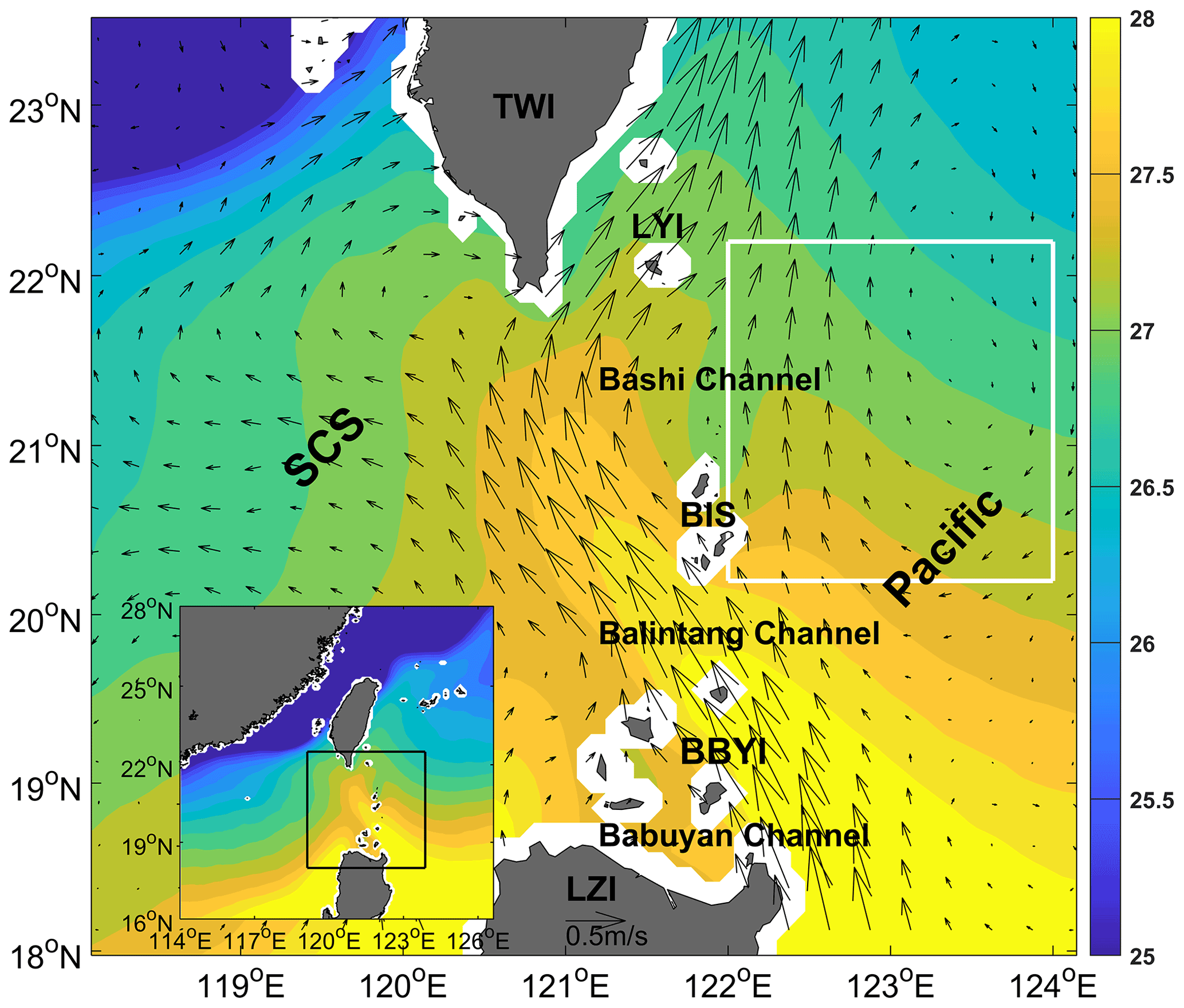
Figure 1 Climate state of spatial distribution of remote sensing systems (RSS, 2022) SST (^∘C; shading) and CMEMS geostrophic current (m s⁻¹; vectors) from 2003 to 2020. SCS, South China Sea; BIS, Batanes Islands; TWI, Taiwan Island; LZI, Luzon Island; BBYI, Babuyan Islands; LYI, Lanyu Island. White box borders 20.2–22.2^∘ N, 122–124^∘ E. Extent of the main map is shown as black-bordered box in inset.

Mesoscale eddy interaction is an important focus of previous studies on mesoscale eddies in the LS. Jing and Li (2003) used satellite remote-sensing observation data to discover a cyclonic mesoscale cold eddy around Lanyu Island to the northeast of the LS. They pointed out that the formation of the Lanyu cold eddy was the result of the joint action of the meandering Kuroshio overshooting and conservation of the potential vorticity. Sun et al. (2016b) believed that the formation of the Lanyu cold eddy was a process of eddy–eddy interaction. They used satellite observation data and composition analysis to study the Lanyu cold-eddy phenomenon, and pointed out that the combined action of the Kuroshio loop (cyclonic circulation) and an AE from the NWP leading to the formation of the Lanyu cold eddy. Based on satellite observation data, in situ observation data and numerical modeling data, Zhang et al. (2017) studied mesoscale eddy–eddy interaction to the northwest of the LS. They analyzed the energy budget of the Kuroshio invading the SCS, and determined that the northern branch of the anti-cyclonic circulation caused by the Kuroshio loop had a large horizontal shear stress and thus led to the formation of a CE southwest of Taiwan Island through the barotropic instability.

Previous studies showed that mesoscale eddy–eddy interaction can cause particle and energy exchange and often occurs in the vicinity of the LS (Sun et al., 2016b; Zhang et al., 2017; Sun et al., 2018). Since the LS is an important gap for particle and energy exchange between the SCS and NWP, a logical question is whether this phenomenon of mesoscale eddy–eddy interaction can occur on the east and west sides of the LS and whether it plays an important role in the particle and energy exchange between the SCS and NWP. To explore this issue, we compare sea-surface height anomaly (SSHA) distributions in the SCS when a CE occurs and when an AE occurs on the east side of the LS (Fig. 2). The specific process is described in detail in Sect. 3.1. Figure 2 shows that when an AE (a CE) occurs on the east side of the LS, a CE (an AE) forms on the west side of the LS, which was observed in the in situ observation data (Huang et al., 2019). This is referred to in this article as the counter-rotating eddy-pair phenomenon.

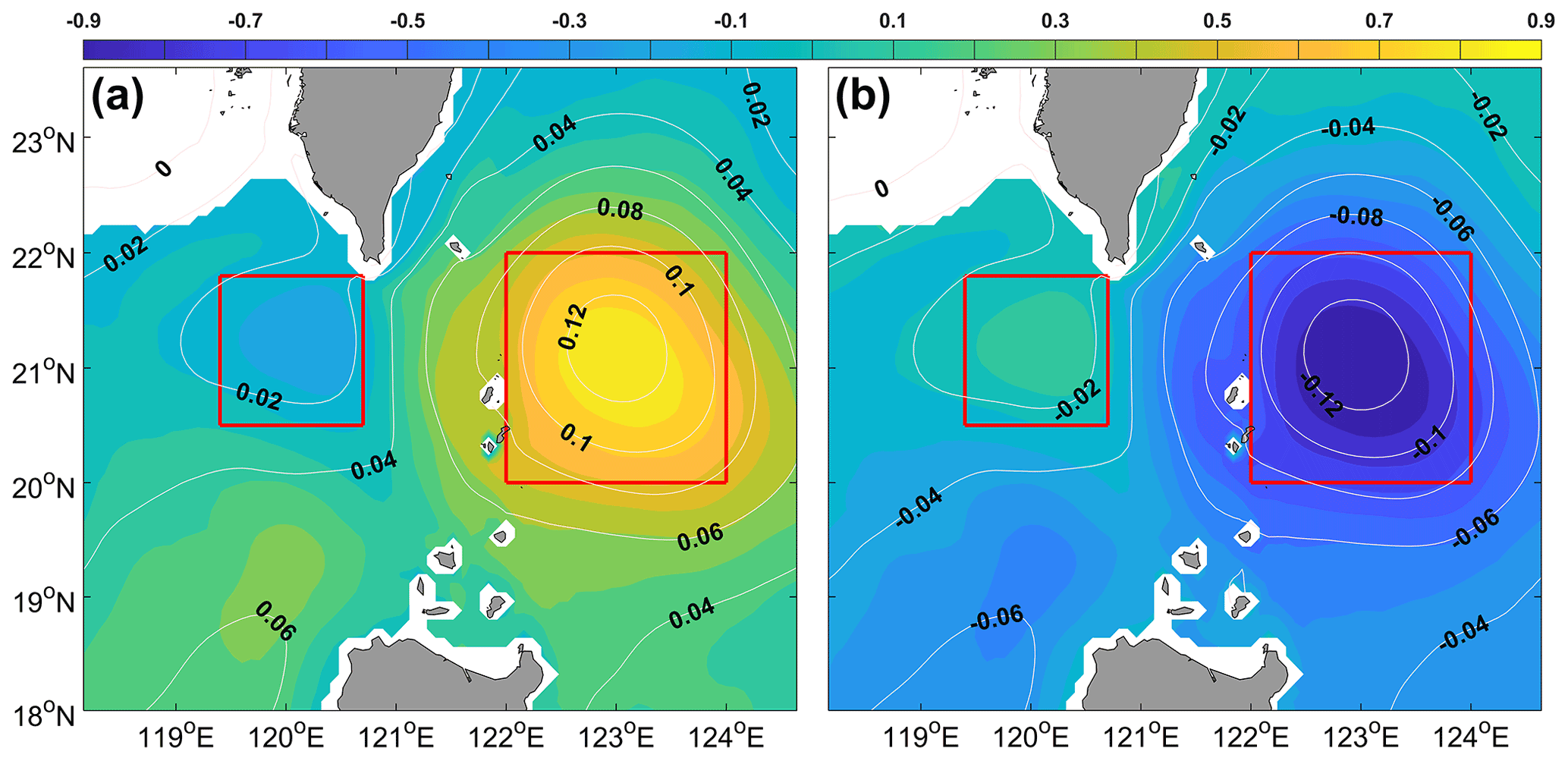
Figure 2 Spatial distribution of counter-rotating eddy pair in the LS. Spatial patterns of AE (a) and CE (b) modes. Panel (a) corresponds to average state when an AE (and b when a CE) occurred in area marked by red box on east side of LS from 1993 to 2020. Contours represent SSHA (units of m). Colors represent sea temperature anomaly (units of ^∘C) at a depth of 300 m. Interval of SSHA is 0.03 m. Red boxes on west and east sides of LS border mark 20.5–21.8^∘ N, 119.4–120.7^∘ E and 20–22^∘ N, and 122–124^∘ E, respectively. Figure is similar to Fig. 3 of Sun et al. (2018), and is based on HYCOM data.

To our knowledge, this is the first time a counter-rotating eddy-pair phenomenon in the LS has been proposed, which creates a new form of particle and energy exchange between the SCS and the NWP. The present study will supplement and fulfill the theory of particle and energy exchange between the SCS and NWP. We give the statistical characteristics and dynamic mechanism of this phenomenon herein. The rest of this paper is organized as follows: Sect. 2 briefly introduces the data and methods, Sect. 3 presents the research results, and Sect. 4 provides a discussion and conclusion.

2 Data and methods

2.1 Data

Satellite remote-sensing SSHA, geostrophic current, and geostrophic current anomaly data were provided by the Copernicus Marine Environment Monitoring Service (CMEMS). The dataset was generated by the processing system including data from all altimeter missions: Sentinel-3A/B, Jason-3, HY-2A, Cryosat-2, OSTM/Jason-2, Jason-1, Topex/Poseidon, Envisat, GFO, and ERS-1/2. The dataset provides global coverage data from 1 January 1993 to 2 August 2021, with a spatial resolution of 0.25^∘ × 0.25^∘ and temporal sampling frequency of 1 d. It also provides one near-real-time component and one delayed-time component. The delayed-time component has been inter-calibrated and provides a homogeneous and highly accurate long time series of all altimeter data (Pujol and Francoise, 2022), and is chosen for use in this paper.

Model data are obtained from the Hybrid Coordinate Ocean Model (HYCOM) model output by the US Naval Research Laboratory. The dataset is based on ocean prediction system output, and the product with the longest time span from 2 October 1992 to 31 December 2012 was chosen from all HYCOM data-assimilation products provided by the HYCOM organization. The dataset is based on ocean prediction system output with a spatial resolution of 0.08^∘ × 0.08^∘ and 40 standard z levels between 80.48^∘ S and 80.48^∘ N. It provides temperature, salinity, sea-surface height, zonal flow, and meridional flow (Wallcraft et al., 2003).

The wind dataset was provided by the National Centers for Environmental Information (NCEI). The dataset merges multiple satellite observations with in situ instrument and related individual products, provides 6 h, daily, and monthly wind and climate data with a spatial resolution of 0.25^∘ × 0.25^∘, and contains globally gridded ocean surface vector winds and wind stresses (Zhang et al., 2006).

Sea surface temperature (SST) data are from remote-sensing systems (RSSs). The dataset merges the near-coastal capability and high spatial resolution of infrared SST data with through-cloud capabilities of microwave SST data, and has applied atmospheric corrections. It provides daily data with a spatial resolution of 9 km × 9 km from 1 July 2002 to the present.

2.2 Methods

2.2.1 Eddy energetic and hydrodynamic instability formula

The formation mechanisms of mesoscale eddies in the ocean are commonly attributed to baroclinic and barotropic instabilities (Pedlosky, 1987). The barotropic conversion (BT) and baroclinic conversion (BC) are manifestations of the baroclinic and barotropic instabilities, respectively, and they are the major eddy energy sources around the LS (Yang et al., 2013; Zhang et al., 2013, 2015, 2017). In addition, the wind-stress work (WW) can also contribute to the formation of eddies (Ivchenko, 1997; Sun et al., 2015). The BT, BC, and WW can be expressed as follows (Ivchenko, 1997; Oey, 2008):

$$\begin{array}{}\text{(1)}& {\displaystyle }\mathrm{BT}=-\int \left(\stackrel{\mathrm{‾}}{u^{\prime \mathrm{2}}}{\displaystyle \frac{\partial \stackrel{\mathrm{‾}}{u}}{\partial x}}+\stackrel{\mathrm{‾}}{v^{\prime \mathrm{2}}}{\displaystyle \frac{\partial \stackrel{\mathrm{‾}}{v}}{\partial y}}+\stackrel{\mathrm{‾}}{u^{\prime }{v}^{\prime }}{\displaystyle \frac{\partial \stackrel{\mathrm{‾}}{u}}{\partial y}}+\stackrel{\mathrm{‾}}{u^{\prime }{v}^{\prime }}{\displaystyle \frac{\partial \stackrel{\mathrm{‾}}{v}}{\partial x}}\right)\mathrm{d}z,\text{(2)}& {\displaystyle }\mathrm{BC}=-\int {\displaystyle \frac{g^{\mathrm{2}}}{{\mathit{\rho }}_{\mathrm{0}}^{\mathrm{2}}{N}^{\mathrm{2}}}}\left(\stackrel{\mathrm{‾}}{u^{\prime }{\mathit{\rho }}^{\prime }}{\displaystyle \frac{\partial \stackrel{\mathrm{‾}}{\mathit{\rho }}}{\partial x}}+\stackrel{\mathrm{‾}}{v^{\prime }{\mathit{\rho }}^{\prime }}{\displaystyle \frac{\partial \stackrel{\mathrm{‾}}{\mathit{\rho }}}{\partial y}}\right)\mathrm{d}z,\text{(3)}& {\displaystyle }\mathrm{WW}={\displaystyle \frac{\mathrm{1}}{\mathit{\rho }}}\left(\stackrel{\mathrm{‾}}{u^{\prime }{\mathit{\tau }}_x^{\prime }}+\stackrel{\mathrm{‾}}{v^{\prime }{\mathit{\tau }}_y^{\prime }},\right).\end{array}$$

where t is time; u, v, and w are the zonal velocity, meridional velocity, and vertical velocity, respectively, and their positive directions are east, north, and up, respectively. g is the acceleration due to gravity; N is the buoyancy frequency; ρ is the density of seawater; ρ₀=1030 kg m⁻³ is the mean seawater density; p is the sea pressure; and τ_x and τ_y are the zonal and meridional components of the wind stress, respectively. x, y, and z are the conventional east–west, north–south, and up–down Cartesian coordinates, respectively. The depth integrals for BT and BC are from 400 m to the sea surface. The overbar denotes a time average over 70 d, the primes denote deviations from the average value of 35 d before and after this day, and the other symbols and notations are standard. From Figs. 6 and 8, it can be seen that the counter-rotating eddy-pair phenomenon occurs, develops, and disappears from $t=-\mathrm{36}$ to t=36, i.e., approximately 70 d. Therefore, the period is chosen to be 70 d. We have made several attempts to set the period between 65 and 80 d, and they did not affect our basic conclusion. BT and BC were calculated from HYCOM data. CMEMS surface-current velocity data and NCDC wind data were used to calculate WW.

2.2.2 Vorticity budget equation

To examine the influence of the vorticity change, we applied the vorticity budget equation (Muller, 1995; Kuo and Tseng, 2021):

$$\begin{array}{}\text{(4)}& \begin{array}{rl}{\displaystyle \frac{\partial \mathit{\zeta }}{\partial t}}& =-u{\displaystyle \frac{\partial \mathit{\zeta }}{\partial x}}-v{\displaystyle \frac{\partial \mathit{\zeta }}{\partial y}}-\left(\mathit{\zeta }+f\right)\mathrm{\nabla }\mathit{u}-v{\displaystyle \frac{\partial f}{\partial y}}\\ & +{\displaystyle \frac{\mathrm{1}}{{\mathit{\rho }}^{\mathrm{2}}}}\left({\displaystyle \frac{\partial \mathit{\rho }}{\partial x}}{\displaystyle \frac{\partial P}{\partial y}}-{\displaystyle \frac{\partial \mathit{\rho }}{\partial y}}{\displaystyle \frac{\partial P}{\partial x}}\right)-\mathit{\upsilon }{\displaystyle \frac{{\partial }^{\mathrm{2}}\mathit{\zeta }}{{\partial }^{\mathrm{2}}z}},\end{array}\end{array}$$

where $\mathit{\zeta }=\frac{\partial v}{\partial x}-\frac{\partial u}{\partial y}$ is the relative vorticity, t is time, f is the Coriolis parameter, P is the seawater pressure, and $\mathit{\upsilon }=\mathrm{1.004}\times {\mathrm{10}}^{-\mathrm{6}}$ is the kinematic viscosity coefficient. x, y, z, u, v, and ρ in Eq. (4) are defined as in Eqs. (1)–(3). The items on the right-hand side of the equation are, from left to right, the zonal advection, meridional advection, stretching, beta, baroclinic, and diffusion terms.

2.2.3 Definition of modes and intensity index of counter-rotating eddy-pair phenomenon

When an AE (a CE) in the NWP gradually approaches the northern LS, a CE (an AE) gradually forms on the west side of the LS, and we define it as an AE (a CE) mode of the counter-rotating eddy-pair phenomenon, as shown in Figs. 2a, 3a, and 6 (Figs. 2b, 3b, and 8).

To reflect the intensity of counter-rotating eddy-pair phenomenon, we must construct an intensity index. As this phenomenon mainly involves the difference of SSHA between the east and west sides of the LS, the index is defined as the time series of the SSHA in the east red box of Fig. 2 (expressed as SSHA_east) minus that in the west red box of Fig. 2 (expressed as SSHA_west), which is shown in Fig. 3a and can be expressed as $\mathrm{Index}={\mathrm{SSHA}}_{\mathrm{east}}-{\mathrm{SSHA}}_{\mathrm{west}}$.

3 Results

3.1 Identification of counter-rotating eddy pair in LS

Based on cluster analysis, which is the same as the clustering method used by Sun et al. (2018), the SSHA and sea-temperature anomaly (STA) are determined based on the days when an AE and a CE exist on the east side of the LS (shown in the white box in Fig. 1), respectively. Figure 2a shows that the SSHA in the red box on the east side of the LS increases from the outside to inside, which means that there is an AE. Owing to geostrophic balance and mass conservation, the AE causes convergence of sea water, leading to down-welling in its center, subsequently leading to an increase in the temperature in the deep ocean. This is verified by the fact that the STA in the red box on the east side of the LS gradually increases from outside to inside and the value is highest in the center. In addition, the SSHA in the red box on the west side of the LS decreases from outside to inside and the STA is negative, indicating the presence of a weak CE. According to the definition of modes of the counter-rotating eddy pair given in Sect. 2.2.3, the SSHA pattern in Fig. 2a can be identified as an AE mode of the counter-rotating eddy pair.

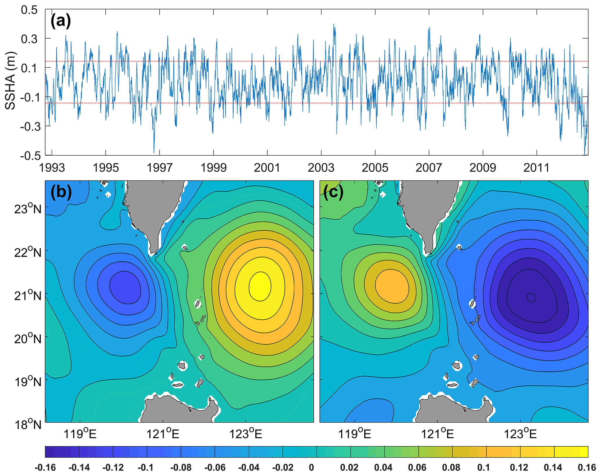
Figure 3 Time series of intensity index of counter-rotating eddy pair in LS (a). Red dotted line above (below) represents the sum (difference) of one time the standard deviation and the average value of the time series. Composition of SSHA for positive (b) and negative (c) intensity-index days. SSHA interval is 0.02 m. Figure based on HYCOM data.

Figure 2b is similar to Fig. 2a, but for a CE and an AE on the east and west sides of the LS, respectively, its SSHA pattern can be identified as an AE mode of the counter-rotating eddy pair. According to the intensity index defined in Sect. 2.2.3, the SSHA is constructed based on the days when the positive and negative intensity index values are more than one standard deviation from the mean, as shown in Fig. 3b and c. Figure 3b (Fig. 3c) shows that an AE (a CE) on the east side of the LS corresponds well to a CE (an AE) on the west side of the LS, and can well reflect the AE (CE) mode of a counter-rotating eddy pair in the LS. It also shows that we can well identify this phenomenon according to the intensity index, and, furthermore, that the positive and negative intensity indexes correspond to AE and CE modes, respectively, of this phenomenon.

3.2 Seasonal variation of counter-rotating eddy pair in LS

We counted the temporal distribution of the positive and negative intensity index values in a statistical sense. Figure 4a (Fig. 4b) shows that most of the AE (CE) mode of the instances of the counter-rotating eddy pair occur in the summer (winter) half of the year. The first two months with the highest incidences of the AE (CE) mode are May and June (December and January), and their occurrence rates are 17.01 % and 15.47 % (19.69 % and 15.57 %), respectively. We constructed the geostrophic current in May and June (Fig. 5a) and in December and January (Fig. 5b). The patterns of the Kuroshio Current in Fig. 5a and b exhibit as the “Leap” and “Loop” patterns of the Kuroshio in the LS, which illustrates that the Leap and Loop patterns of the Kuroshio contribute to the occurrence of the AE and CE modes, respectively, of the counter-rotating eddy pair. Figure 5c (Fig. 5d) shows that the geostrophic current anomaly in the northern LS is northward (southward). It produces positive (negative) vorticity through horizontal velocity shear on the west side of the LS, and then contributes to the formation of a CE (an AE) on the west side of the LS. We discuss the dynamic mechanism of the counter-rotating eddy-pair phenomenon in detail in Sect. 3.3.

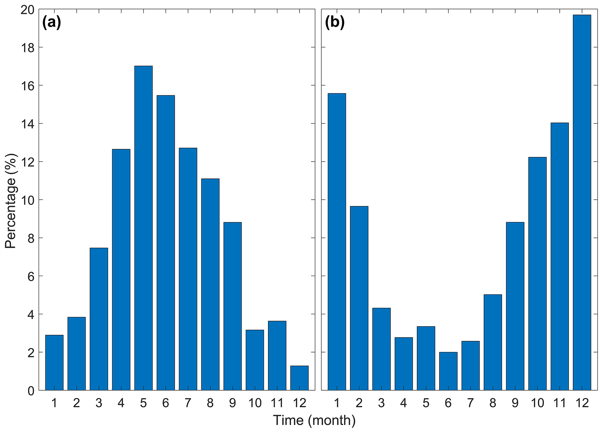
Figure 4 Seasonal distribution of occurrence rate for positive (a) and negative (b) intensity indexes.

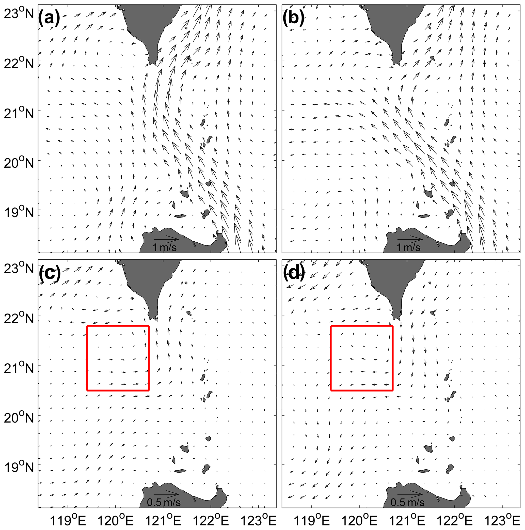
Figure 5 Climatic distributions of geostrophic current in May and June (a) and in December and January (b), and of geostrophic current anomaly in May and June (c) and in December and January (d). Red boxes in (c) and (d) outline 20.5–21.8^∘ N, 119.4–120.7^∘ E, which represent the position of mesoscale eddies on west side of LS. Figure based on CMEMS data.

3.3 Evolution of counter-rotating eddy pair in LS

Figure 6 shows the spatial evolution of the AE mode of the counter-rotating eddy pair in the LS. It shows that at the beginning, for example, at $t=-\mathrm{24}$, there is a weak AE far from the east side of the LS, but no CE on the west side of the LS. From $t=-\mathrm{20}$ to t=0, as the AE in the NWP approaches the northern LS, a CE gradually forms on the west side of the LS. At t=0, the AE mode reaches its maximum. Then, from t=4 to t=36, as the AE in the NWP gradually moves away from the northern LS, the CE on the west side of the LS gradually weakens until it finally dies out.

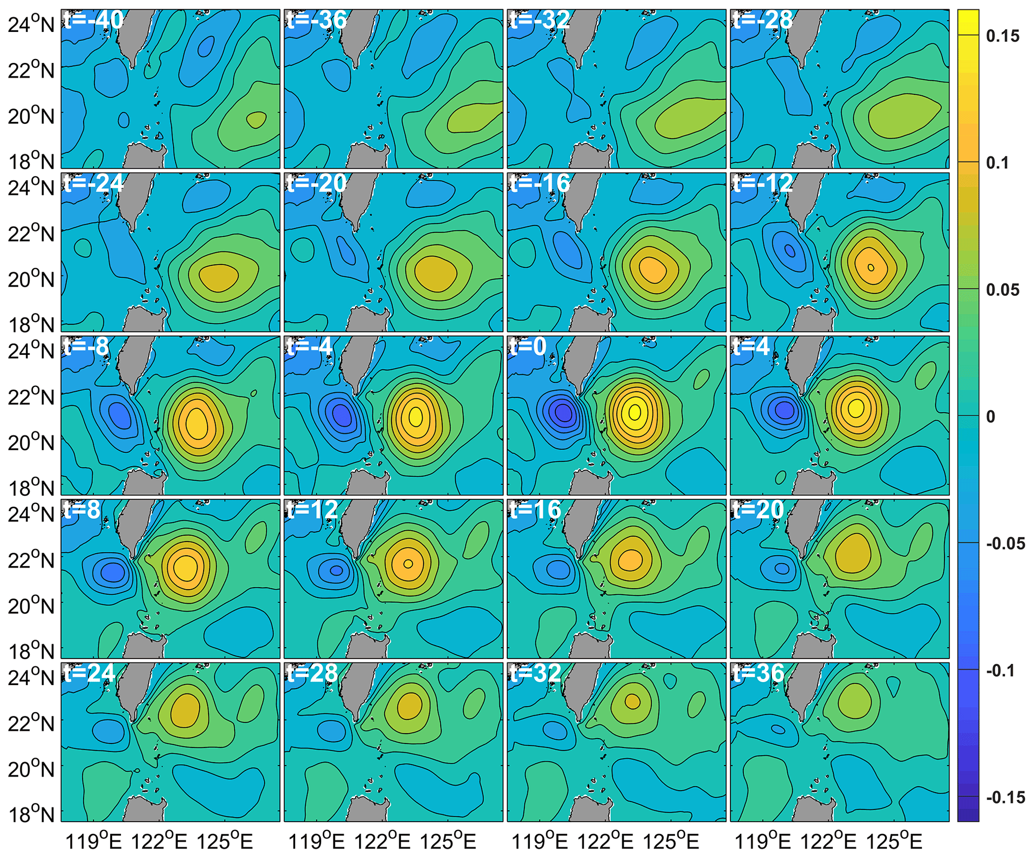
Figure 6 Evolution of AE mode of counter-rotating eddy pair in LS based on HYCOM data. Contours and shading both represent SSHA (units of m). SSHA interval is 0.02 m. t value in the top left-hand corner of each panel denotes the days before (negative value) or after (positive value) AE mode of counter-rotating eddy pair reached the maximum (t=0). t=0 corresponds to the time of Fig. 3b.

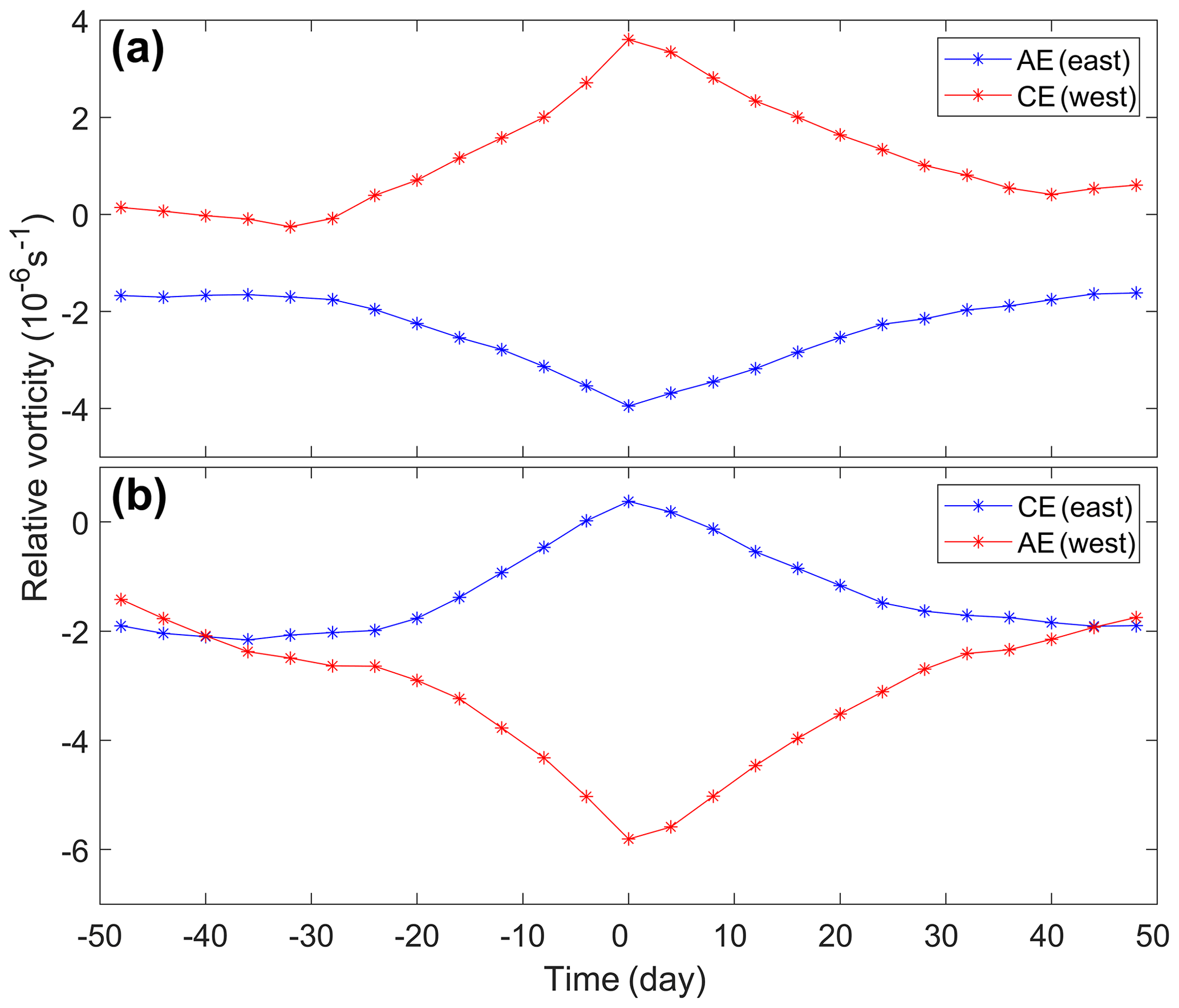
Figure 7 Distribution of relative vorticity in area bordered by red boxes in Fig. 2. (a) Relative vorticity of AE mode over time. Blue (red) line represents time series of relative vorticity of AE (CE) on east (west) side of LS, which corresponds to Fig. 6. (b) Relative vorticity of CE mode over time. Blue (red) line represents time series of relative vorticity of CE (AE) on east (west) side of LS, which corresponds to Fig. 8. Figure based on HYCOM data.

The growth and weakening of a mesoscale eddy must be accompanied by a change in its relative vorticity. Figure 7a shows that as the AE on the east side of the LS approaches and then moves away from the northern LS, its relative vorticity initially decreases and then increases, while the relative vorticity of the corresponding CE on the west side of the LS initially increases and then decreases. The maximum negative (positive) value of the time series of the AE (CE) on the east (west) side of the LS reaches $-\mathrm{4.2}\times {\mathrm{10}}^{-\mathrm{6}}$ s⁻¹ ($\mathrm{3.6}\times {\mathrm{10}}^{-\mathrm{6}}$ s⁻¹). These time series have good correspondence and their correlation coefficient is −0.97 at the 95 % confidence level. Therefore, the temporal variations in the relative vorticity in Fig. 7a verify the evolution of the AE mode of the counter-rotating eddy pair in the LS.

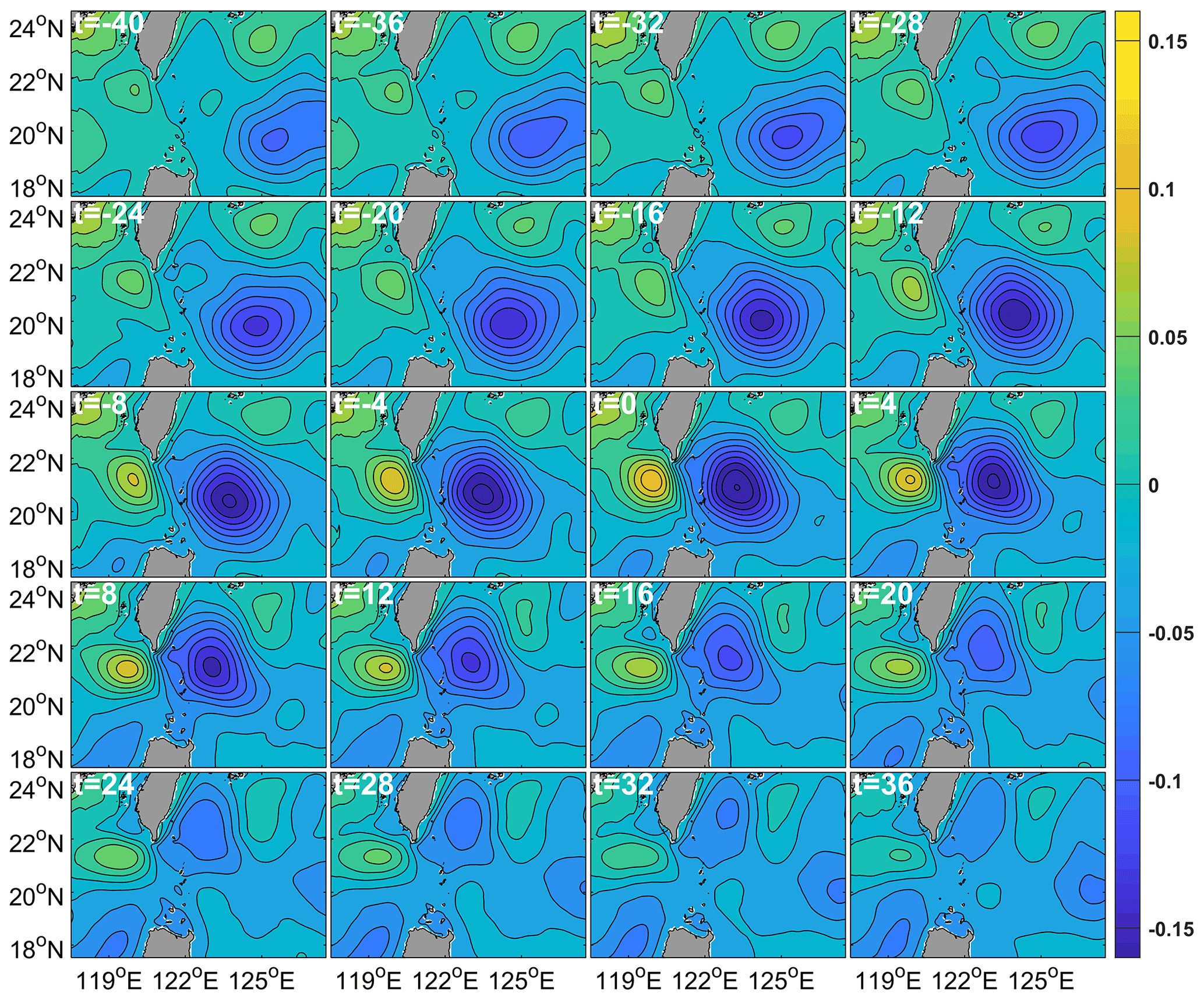
Figure 8 Evolution of CE mode of counter-rotating eddy pair in LS based on HYCOM data. Contours and shading both represent SSHA (units of m). SSHA interval is 0.02 m. t in the top left-hand corner of each panel denotes the days before (negative value) or after (positive value) the CE mode of the counter-rotating eddy pair reached the maximum (t=0). t=0 corresponds to time of Fig. 3b.

Figure 8 plots the CE mode of the counter-rotating eddy pair in the LS. It shows that at the beginning, for example, at $t=-\mathrm{32}$, there is a weak CE far from the east side of the LS, but no AE on the west side of the LS. From $t=-\mathrm{28}$ to t=0, as the CE in NWP approaches the northern LS, an AE gradually forms on the west side of the LS. At t=0, the CE mode of the evolution of the counter-rotating eddy pair reaches the maximum. Then, from t=4 to t=36, as the CE in the NWP gradually moves away from the northern LS, the AE in the west side of the LS gradually weakens until it finally dies out. Figure 7b plots the CE mode and shows that as the CE on the east side of the LS approaches and moves away from the northern LS, its relative vorticity initially increases and then decreases, while the relative vorticity of the corresponding AE on the west side of the LS initially decreases and then increases. The maximum positive (negative) value of the time series of the CE (AE) on the east (west) side of the LS can reach $\mathrm{0.48}\times {\mathrm{10}}^{-\mathrm{6}}$ s⁻¹ ($-\mathrm{6.7}\times {\mathrm{10}}^{-\mathrm{6}}$ s⁻¹). These time series have good correspondence and their correlation coefficient is −0.96 at the 95 % confidence level. Therefore, the temporal variations in the relative vorticity in Fig. 7b verify the evolution of the AE mode of the counter-rotating eddy pair in the LS. The evolution of the AE and CE modes of the counter-rotating eddy pair in the LS is also reflected by the satellite observations (Figs. 9 and 10).

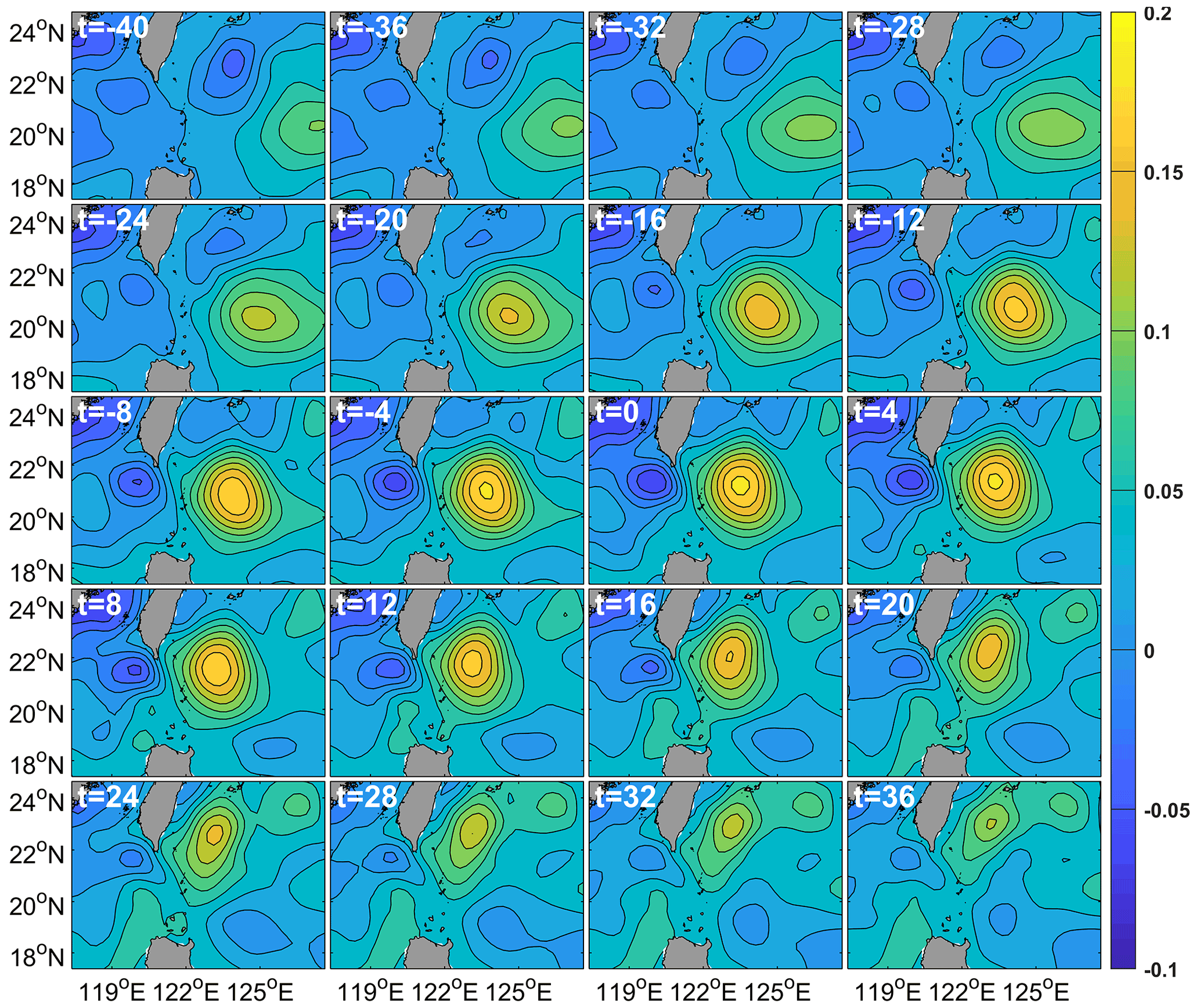
Figure 9 Evolution of AE mode of counter-rotating eddy pair in LS based on CMEMS data. Contours and shading both represent SSHA (units of m). SSHA interval is 0.02 m. t in the top left-hand corner of each panel denotes days before (negative value) or after (positive value) the AE mode of counter-rotating eddy pair reached the maximum (t=0). t=0 corresponds to time of Fig. 3b.

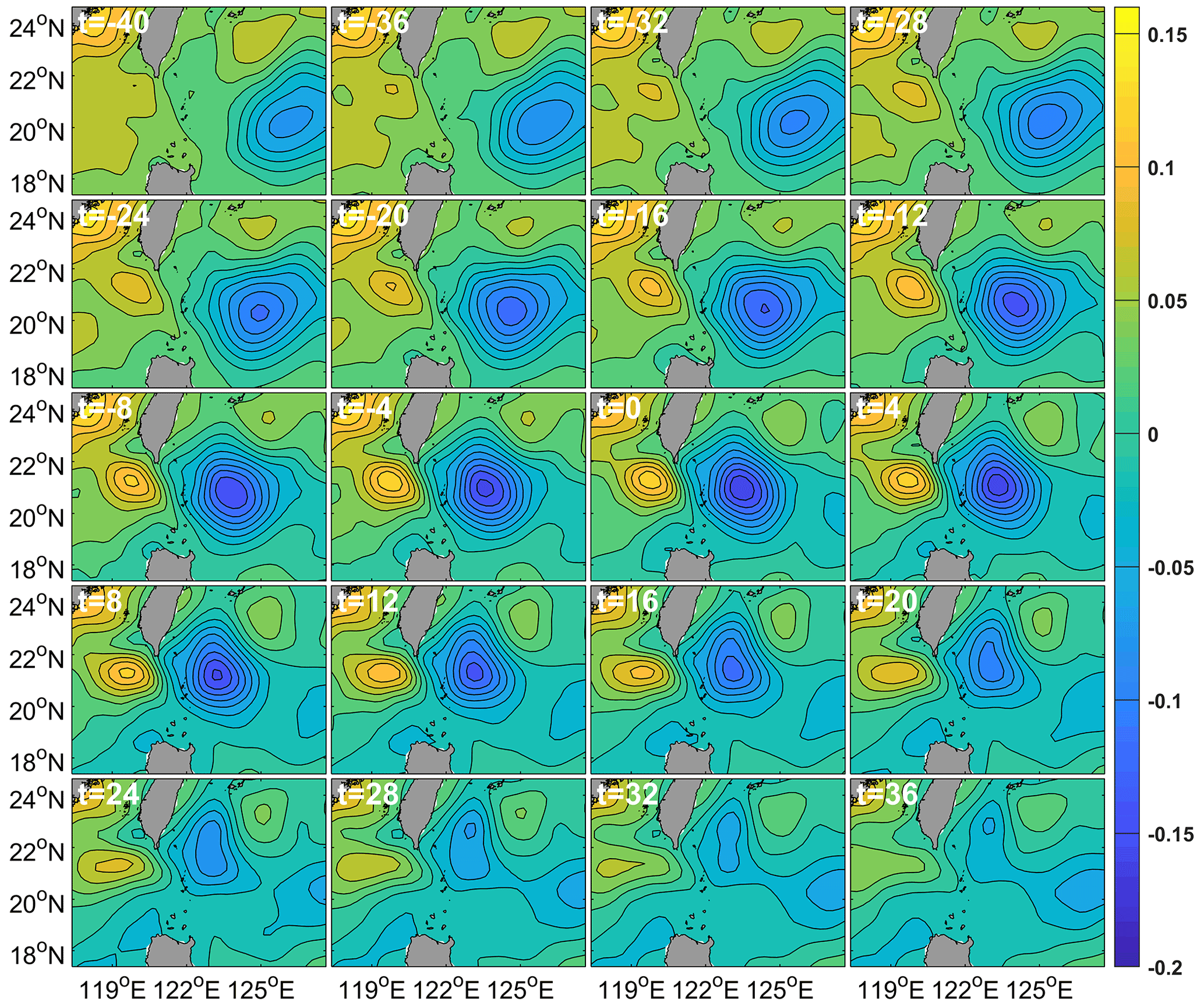
Figure 10 Evolution of CE mode of counter-rotating eddy pair in LS based on CMEMS data. Contours and shading both represent SSHA (units of m). SSHA interval is 0.02 m. t in the top left-hand corner of each panel denotes days before (negative value) or after (positive value) the CE mode of counter-rotating eddy pair reached the maximum (t=0). t=0 corresponds to time of Fig. 3b.

3.4 Formation mechanism of counter-rotating eddy pair in LS

Zhang et al. (2017) reported that CEs mainly formed due to the barotropic instability caused by horizontal velocity shear of the Kuroshio Loop current southwest of Taiwan Island. Huang et al. (2019) discovered that an AE from the NWP caused a CE to form on the west side of the LS via horizontal velocity shear. In addition, Fig. 3b and c show that the dense contour of the SSHA means that there are strong current anomalies and thus strong horizontal velocity shear at the junction of the AE and CE. Therefore, we investigated the role of horizontal velocity shear in the formation of a counter-rotating eddy in the LS.

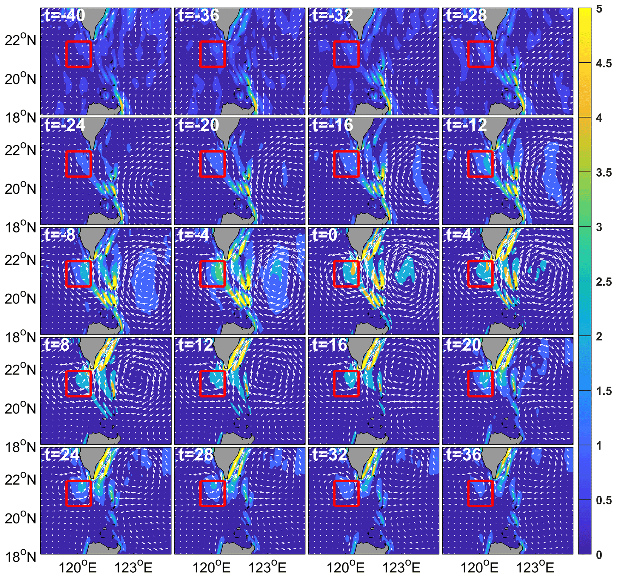
Figure 11 Evolution process of absolute value of zonal horizontal velocity shear ($\frac{\partial v}{\partial x}$) for AE mode of counter-rotating eddy pair in LS based on HYCOM data. Shading represents zonal horizontal velocity shear (units of 10⁻⁶ s⁻²). Vector represents the current anomaly. t in the top left-hand corner of each panel denotes days before (negative value) or after (positive value) the AE mode of counter-rotating eddy pair reached the maximum (t=0). t=0 corresponds to time of Fig. 3b. Red boxes on west side of LS cover 20.5–21.8^∘ N, 119.4–120.7^∘ E and represent location of CE on west side of LS.

Because meridional horizontal velocity shear is weak, we only show the zonal velocity shear. Figure 11 shows that from $t=-\mathrm{40}$ to t=0, as the AE on the east side of the NWP gradually approaches the northern LS, the absolute value of the zonal horizontal velocity shear ($\frac{\partial v}{\partial x}$) gradually increases, and a CE gradually forms and strengthens on the west side of the LS. From t=0 to t=36, as the AE gradually moves away from the northern LS, the absolute value of the zonal horizontal velocity shear gradually decreases, and the CE on the west side of the LS gradually weakens. Figure 12 plots the CE mode of the counter-rotating eddy pair in the LS and shows a similar corresponding evolution process. This demonstrates that there is good correspondence between the zonal horizontal velocity shear and evolution process of the counter-rotating eddy pair.

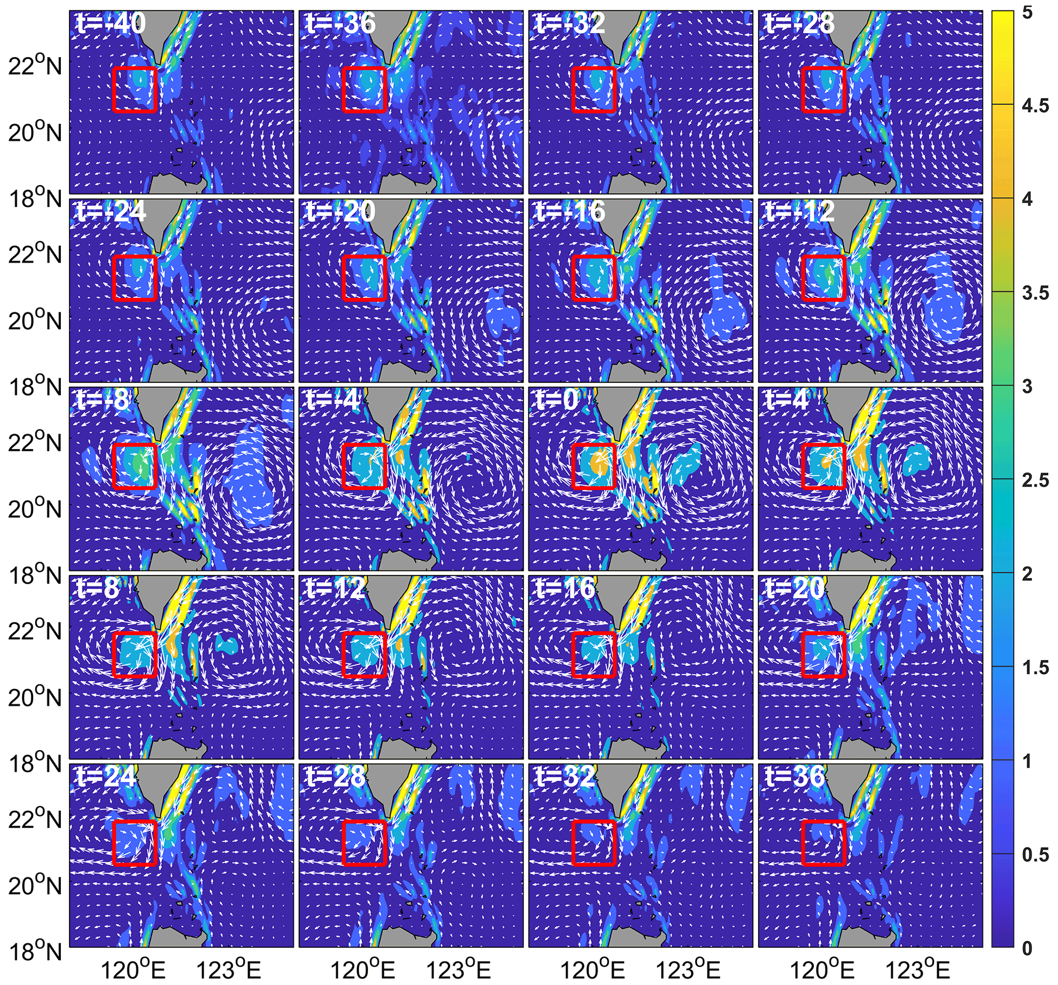
Figure 12 Evolution process of absolute value of zonal horizontal velocity shear ($\frac{\partial v}{\partial x}$) for CE mode of counter-rotating eddy pair in LS based on HYCOM data. Shading represents zonal horizontal velocity shear (units of 10⁻⁶ s⁻²). Vector represents current anomaly. t in top left-hand corner of each panel denotes days before (negative value) or after (positive value) the AE mode of counter-rotating eddy pair reached the maximum (t=0). Time t=0 corresponds to time of Fig. 3b. Red boxes on west side of LS cover 20.5–21.8^∘ N, 119.4–120.7^∘ E and represent the location of CE on west side of LS.

However, Fig. 11 (Fig. 12) shows that zonal horizontal velocity shear only occurs on the right-hand side of the red box; that is, on the right-hand side of the CE (AE). How does the horizontal velocity shear pass to the entire CE (AE)? To answer this question, we used the vorticity budget equation. Figure 13a1–f1 plot the AE mode of the counter-rotating eddy pair and show the respective contributions of the zonal advection, meridional advection, stretching, beta, baroclinic, and diffusion terms of the vorticity budget equation. Compared to the stretching, beta, baroclinic, and diffusion terms, the values of the zonal advection and meridional advection terms in the red box are large. However, most of the values of the meridional advection term in the red box are negative. Only positive vorticity advection can lead to formation of a CE, which suggests that the zonal advection term is the main cause of CE formation in the red box. To further test this conclusion, Fig. 14a shows the correspondence between the relative vorticity anomaly and zonal advection of the vorticity in the red box in Fig. 13, illustrating that there is good correspondence and their correlation coefficient is as high as 0.96 at the 95 % confidence level. Therefore, we conclude that the zonal advection term plays the most important role in vorticity transport and contributes to the formation of the CE on the west side of the LS.

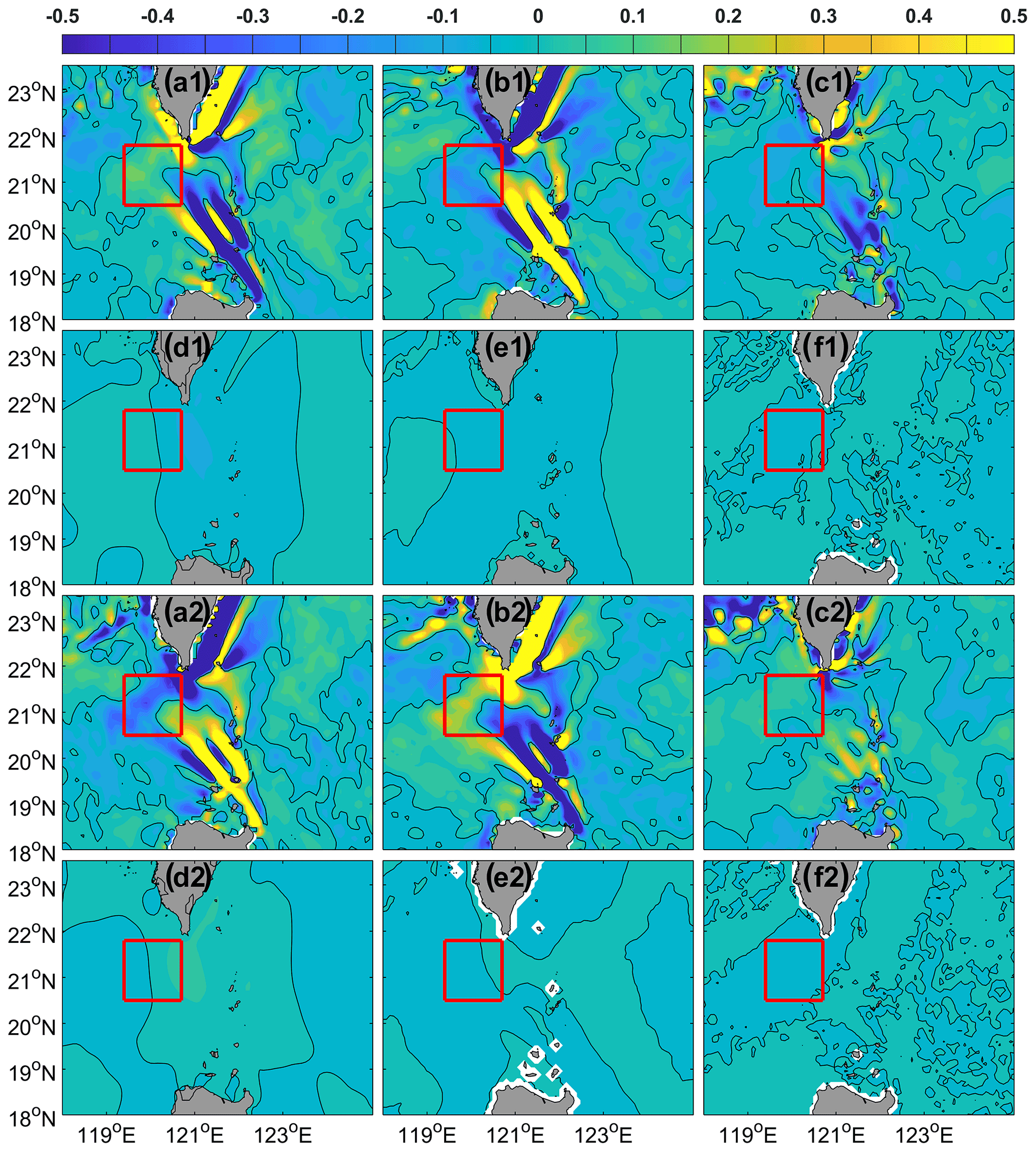
Figure 13 Vorticity budget equation for (a1–f1) AE mode of counter-rotating eddy pair and (a2–f2) CE mode of counter-rotating eddy pair. Panels (a1) and (a2) represent the zonal advection term, (b1) and (b2) the meridional advection term, (c1) and (c2) the stretching term, (d1) and (d2) the beta term, (e1) and (e2) the baroclinic term, and (f1) and (f2) the diffusion term. Units are 10⁻¹⁰ s⁻². Red boxes on west side of LS border cover 20.5–21.8^∘ N, 119.4–120.7^∘ E, and represent location of CE or AE on west side of LS. Black solid line represents the zero contour. Figure based on HYCOM data.

Figure 14 Distribution of relative vorticity anomaly and zonal advection of vorticity surrounded by red boxes in Fig. 13 for AE (a) and CE (b) modes of counter-rotating eddy pair in LS.

Figure 13a2–f2 are plots the CE mode of the counter-rotating eddy pair and shows that, compared to the stretching, beta, baroclinic, and diffusion terms, the values of the zonal advection and meridional advection terms in the red box are large. However, most of the values of the meridional advection term in the red box are positive. Only negative vorticity advection can lead to formation of an AE, which implies that the zonal advection term is the main cause of AE formation in the red box. To further test this conclusion, Fig. 14b shows the correspondence between the relative vorticity anomaly and zonal advection of vorticity, illustrating that there is good correspondence and their correlation coefficient is as high as 0.84 at the 95 % confidence level. Therefore, we conclude that the zonal advection term plays the most important role in vorticity transport and contributes to the formation of the AE on the west side of the LS.

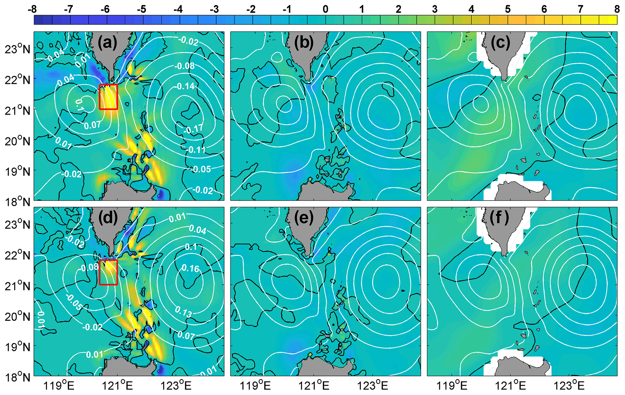
Figure 15 BT based on HYCOM data (10⁻⁵ m³ s⁻³) represented by colors (a, d); BC based on HYCOM data (10⁻⁵ m³ s⁻³) represented by colors (b, e); WW based on CMEMS surface velocity data and NCDC wind data (10⁻⁵ m³ s⁻³) represented by colors (c, f). Red box borders 21–21.8^∘ N, 120.4–121^∘ E. White contours represent SSHA contours of. Panels (a), (b), and (c) plot CE (and d, e, and f plot AE) mode of counter-rotating eddy pair in LS.

It was mentioned above that the horizontal velocity shear caused by the mesoscale eddy on the east side of the LS is transported westward through zonal advection, resulting in the formation of a counter-rotating mesoscale eddy on the west side of the LS. Horizontal velocity shear will inevitably lead to barotropic instability. Now, we verify our conclusion from the perspective of energy. Figure 15a, b, and c show that, compared to the BC and WW values, the BT values in the LS are large and most of the values are positive, especially in the area surrounded by the red box in Fig. 15a, which is the junction of the AE and CE. This means that the BT plays the most important role in formation of the AE on the west side of the LS.

Figure 15d, e, and f show the BT, BC, and WW, respectively, corresponding to the AE mode of the counter-rotating eddy pair in the LS. The description and dynamic mechanism of the AE mode are similar to those of the CE mode of the counter-rotating eddy pair in the LS, so the details will not be discussed here.

4 Discussion and conclusions

In this study, based on satellite observation data and HYCOM re-analysis data, the counter-rotating eddy pair in the LS is investigated. The phenomenon of counter-rotating eddy pairs is defined as the stage when an AE (a CE) in the NWP gradually approaches the northern LS, and a CE (an AE) forms on the west side of the LS. This phenomenon exhibits obvious seasonal variation; that is, the AE mode mainly occurs in the summer half of the year, while the CE mode mainly occurs in the winter half of the year. The mean durations of the AE and CE modes are both approximately 70 d. The Leap and Loop patterns of the Kuroshio Current contribute to the occurrence of the AE and CE modes, respectively, of counter-rotating eddy pairs. Based on the vorticity budget equation and energy analysis, the dynamic mechanism of the occurrence of a counter-rotating eddy pair is as follows. The AE (CE) in the NWP causes a positive (negative) vorticity anomaly through horizontal velocity shear on the west side of the LS, and the positive (negative) vorticity anomaly is transported westward by the zonal advection of the vorticity, finally leading to the formation of a CE (an AE) on the west side of the LS. This conclusion is also verified by barotropic instability based on the energy analysis.

When we investigated the question of how the horizontal velocity shear passes to the entire CE or AE in Sect. 3.4, we found that the magnitudes of the meridional and zonal advection terms are roughly the same. Because the meridional advection term has the opposite effect of CE (AE) formation in the west side of the LS for the AE (CE) mode of the counter-rotating eddy pair, we confirmed that the zonal advection term plays a main role in horizontal velocity shear transportation. However, since the magnitude of the meridional advection term is very large, it may play a role in the ocean dynamic process of the LS, which requires further study.

The results presented in this study are preliminary and several problems require further research. The occurrence probability of a counter-rotating eddy pair in the LS must be determined. The counter-rotating eddy pair phenomenon involves spatiotemporal variations in two mesoscale eddies on both sides of the LS, and it is difficult to provide a quantifiable definition of this phenomenon for a single event. For example, how far apart must the mesoscale eddies on the east and west sides of the LS be to define them as a counter-rotating eddy pair. We preliminarily calculated that the incidence of this phenomenon is approximately 5 %.

Another problem to solve involves threshold of the NWP mesoscale eddies entering the SCS, and what role the Kuroshio Current plays in the counter-rotating eddy-pair phenomenon in the LS. In this study, our illustration of the counter-rotating eddy pair phenomenon does not include the mean current field, which means that the influence of the Kuroshio Current is not considered. However, the role of the Kuroshio in energy transfer is still worthy of further study. Numerical simulations can be useful to address this issue. Our study provides new perspective on particle and energy exchange, and further perfects the theory of particle and energy exchange between the SCS and NWP.