Simultaneous estimation of ocean mesoscale and coherent internal tide sea surface height signatures from the global altimetry record

This study proposes an approach to estimate the ocean sea surface height signature of coherent internal tides from a 25-year along-track altimetry record, with a single inversion over time, resolving both internal tide contributions and mesoscale eddy variability. The inversion is performed on a reduced-order basis of topography and practically achieved with a conjugate gradient. The particularity of this approach is to mitigate the potential aliasing effects between mesoscales and internal tide estimation from the uneven altimetry sampling (observing the sum of these components) by accounting for their statistics simultaneously, while other methods generally use a prior mesoscale. The four major tidal components are considered (M2, K1, S2, O1) over the period 1992–2017 on a global configuration. From the solution, we use altimetry data after 2017 for independent validation in order to evaluate the performance of the simultaneous inversion and compare it with an existing model.

1 Introduction

Ocean internal gravity waves forced by barotropic tidal currents, known as internal tides, have signatures on sea surface height (SSH) at scales below 200 km (e.g., Ray and Mitchum, 1997). Their vertical extension splits in several modes with specific propagations affected by vertical stratification. These waves, generated in phase with the barotropic tidal current, can remain phase-locked (hereafter called coherent) or phase-modulated by seasonal (Xinhua et al., 2020; Zhao, 2021) or mesoscale (Ponte and Klein, 2015) variability. In particular, the phase-modulated fraction of energy would exceed 50 % in equatorial regions and western boundary currents, as suggested by Zaron (2017) in their Fig. 9. This part would be challenging to resolve from the present along-track altimetry record. However, the coherent part can be estimated from the series of more than 25 years; several empirical approaches have been developed so far, from harmonic analysis (Ray and Zaron, 2016) to a more sophisticated plane wave fit (Zhao, 2019; Zaron, 2019). Data assimilative ocean general circulation models are also able to resolve internal tides (Arbic et al., 2018) with realistic amplitude, but their phase prediction seems not yet as accurate as the empirical approaches mentioned above, as reported in Carrere et al. (2021).

For the sake of improving the empirical approaches, in this study we propose to tackle the issue of mesoscale aliasing in internal tide estimation. Indeed, the mesoscale signal is overall an order of magnitude above internal tides (the typical amplitudes of the latter being as small as ∼2 cm), potentially introducing some aliasing effects when observed by a constellation of a nadir satellites. To mitigate this issue, most approaches use separate estimates of mesoscales such as the DUACS maps distributed by AVISO and CMEMS (Taburet et al., 2019) to subtract the altimetry data used for internal tide analysis. However, it is known that these mesoscale maps may also be contaminated themselves by internal tide aliasing (Zaron and Ray, 2018), potentially affecting the final estimations. In this present study, we propose a simultaneous estimation of mesoscales and internal tides to optimize the mutual aliasing issues. It is based on a single massive inversion over large temporal windows, achieved thanks to a mode decomposition in reduced rank.

In the first section, we present the principle of the simultaneous estimation, with illustrations from idealized one-dimensional synthetic signals. Then, in Sect. 2, the application to altimetry data through the mode decomposition is detailed, followed by the results and validation with independent data. Finally, we will discuss its potential, in particular to handle non-stationary internal tides with future wide-swath altimetry data.

2 Simultaneous estimation: principle and illustrations

The estimation of pure harmonics from partial observations with errors or additional signals is generally performed with harmonic analysis. However, this inversion does not account for particular spatial covariances of the errors or additional signals. When additional errors are white random noise, the impact is minimized and harmonic analysis remains most optimal. However, when we have the knowledge of covariances for the additional signals, especially if they are non-zero between observation coordinates, the estimation can be improved with a full consideration of the signals in the inversion.

2.1 General principle

Here, we present the general inversion formula of a sum of N independent signals of different nature.

We assume N state vectors to be estimated, ${\mathbf{x}}_{\mathbf{k}},k=\mathrm{1}\mathrm{\dots }N$ and partial observations y of the sum of the components, which can be written as follows:

$$\begin{array}{}\text{(1)}& \mathbf{y}=\sum _{\mathbf{k}=\mathbf{1}}^{\mathbf{N}}{\mathbf{H}}_{\mathbf{k}}{\mathbf{x}}_{\mathbf{k}}+\mathit{ϵ},\end{array}$$

where H_k are the observation linear operators and ϵ is an observation error.

If we note $\mathbf{H}=[{\mathbf{H}}_{\mathbf{1}},\mathrm{\dots },{\mathbf{H}}_{\mathbf{N}}]$ and $\mathbf{x}=[{\mathbf{x}}_{\mathbf{1}}^{\mathbf{T}},\mathrm{\dots },{\mathbf{x}}_{\mathbf{N}}^{\mathbf{T}}{]}^{\mathbf{T}}$, then the observation vector can be written as follows: $\mathbf{y}=\mathbf{Hx}+\mathit{ϵ}$, and the application of the optimal interpolation (OI) formula gives

$$\begin{array}{}\text{(2)}& {\mathbf{x}}^{\mathbf{a}}={\mathbf{BH}}^{\mathbf{T}}({\mathbf{HBH}}^{\mathbf{T}}+\mathbf{R}{)}^{-\mathbf{1}}\mathbf{y},\end{array}$$

where B is the covariance matrix of x and R the covariance matrix of error ϵ.

If we assume that the x_k are uncorrelated for the different k so that there are no cross-covariances between the components, the matrix B can be written as follows:

$$\begin{array}{}\text{(3)}& \mathbf{B}=\left[\begin{array}{ccc}{\mathbf{B}}_{\mathbf{1}}& \mathrm{\dots }& \mathrm{0}\\ \mathrm{⋮}& \mathrm{\ddots }& \mathrm{⋮}\\ \mathrm{0}& \mathrm{\dots }& {\mathbf{B}}_{\mathbf{N}},\end{array}\right]\end{array}$$

where the B_k are the covariances for x_k.

2.2 Illustrations

The formulation presented above can be easily tested on a one-dimensional synthetic case, in particular to evaluate the gain of the simultaneous inversion as presented, rather than separate inversions. Let us consider a one-dimensional signal, constituted by the sum of a broadband component following the spectrum shown in black in Fig. 1a (whose integral equals 1), and a pure harmonic of amplitude 1 as represented in gray in the same panel. A signal with these characteristics can be randomly generated following the method described in Ubelmann et al. (2014), Annex 1, assuming random and independent phases between Fourier harmonics. One example is represented in Fig. 1b by the thick black curve for the broadband component and by the thin gray curve for the sum of the two components.

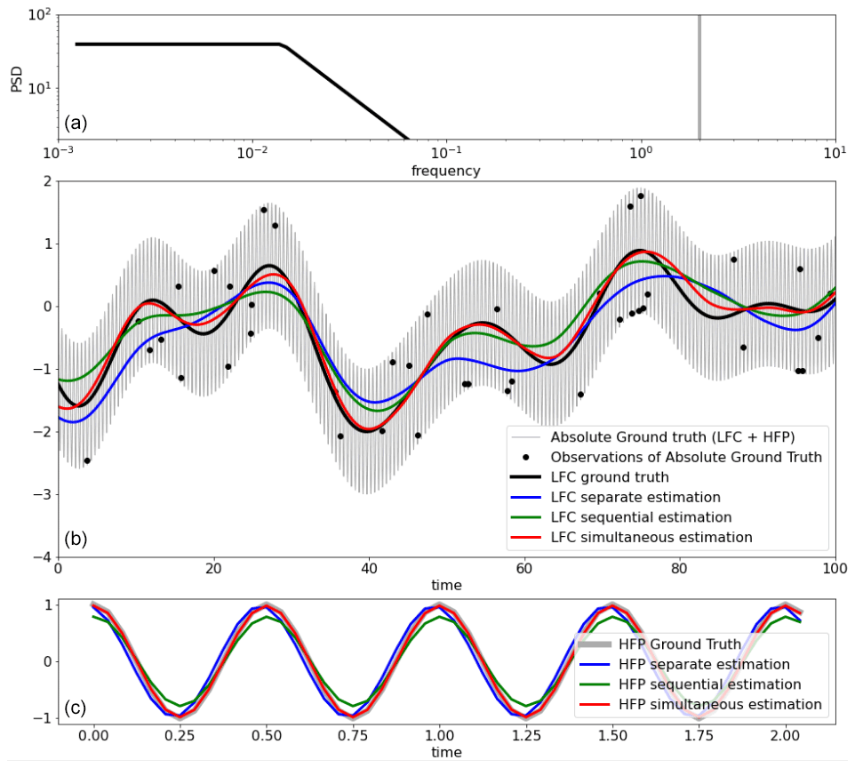
Figure 1 (a) Power spectral density of the ground-truth one-dimensional signal, constituted by a low-frequency continuum (black line) and by a high-frequency peak representing a single harmonic of unitary amplitude. (b) Time series of the ground truth (generated randomly following spectra in (a)) in gray, with the low-frequency component (LFC) shown by the black line, and its three estimations (in colors as indicated in the legend) from the synthetic observations represented by the black dots. (c) Time series of the high-frequency ground truth with its three estimations (in colors as indicated in the legend).

Now let us assume partial observations of this total signal, as represented by the black dots in the figure, here at random times, with typical occurrences of 3 to 5 days and random observation errors of 0.01.

From these observations, we will illustrate the simultaneous inversion method applied to the two components (N=2 in Eqs. 1 to 3), compared to separate estimations.

For the broadband part, k=1, the state vector x₁ is the broadband signal in the 1D grid. H₁ is a linear interpolator of x₁ on the observation coordinates. The covariance matrix B₁ is written in the grid space, with values following the covariance function given by the inverse Fourier transform of the signal spectrum. In this example, it is therefore perfectly optimal.

For the narrowband part, k=2, since we search here for a single harmonic, the state vector x₂ can be reduced to vector of two elements, representing the amplitudes of a sine and cosine, respectively. If t_o is the vector of observation time coordinates, the observation operator H₂ can be written as follows:

$$\begin{array}{}\text{(4)}& {\mathbf{H}}_{\mathbf{2}}=\left[\begin{array}{cc}\cos \left(\mathit{\omega }{\mathbf{t}}_{\mathbf{o}}\right),& \sin \left(\mathit{\omega }{\mathbf{t}}_{\mathbf{o}}\right)\end{array}\right],\end{array}$$

and the covariance matrix B₂ of size 2 by 2 for x₂ can be written as follows:

$$\begin{array}{}\text{(5)}& {\mathbf{B}}_{\mathbf{2}}=\left[\begin{array}{cc}{\mathit{\sigma }}_{\mathrm{2}}^{\mathrm{2}}& \mathrm{0}\\ \mathrm{0}& {\mathit{\sigma }}_{\mathrm{2}}^{\mathrm{2}},\end{array}\right]\end{array}$$

where σ₂ is the expected variance of the harmonic signal.

We used Eq. (2) to estimate simultaneously $\mathbf{x}=[{\mathbf{x}}_{\mathbf{1}},{\mathbf{x}}_{\mathbf{2}}]$ from the vector of observations y, with a diagonal R matrix consistent with the 0.01 STD random error added to the observations.

In parallel, we run the so-called “separate estimations”, where the inversions are applied separately for x₁ and x₂ (with B₁ and B₂ covariance matrices, respectively) and an R matrix accounts for observation error plus the representativity error of the unconsidered component. For the harmonic part, this separate estimation performs nearly as a harmonic analysis, except that the finite B and non-zero R matrices tend to slightly reduce noise contamination with respect to harmonic fit.

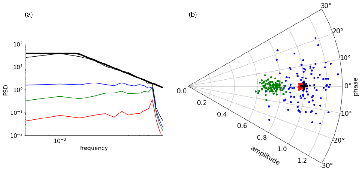
Figure 2 (a) Mean (averaged over the 100 realizations) power spectral densities of the LFC ground truth (thin black) and the LFC estimation error (estimation minus ground truth) for all three estimations (independent, sequential and simultaneous in blue, green and red, respectively). The thick black curve represents the theoretical LFC ground-truth spectrum. (b) Amplitude and phase (in the complex domain) of the high frequency component (HFC), represented by the black cross for the ground truth, and by the green, blue and red points for the 100 realizations of the independent, sequential and simultaneous estimations, respectively.

We also run the so-called “sequential estimations”, consisting of separate estimations with a modified vector of observation, whom the separate estimation of the unconsidered component has been removed. Note that this sequential estimation is similar to what is generally done for internal tide estimations with previous removal of mesoscale signal (e.g., CMEMS/AVISO mesoscale maps).

The results of the different solutions are shown in Fig. 1, in blue for the separate estimations, in green for the sequential estimations and in red for the simultaneous estimations. Qualitatively, the separate estimations clearly suffer from aliasing, for instance the blue curve in Fig. 1b (broadband estimation) is skewed toward observations affected by a given phase of the harmonic signal at the time of observation (high- to low-frequency aliasing). Similarly, the harmonic estimation is affected by the broadband signal values at the time of observations (low- to high-frequency aliasing). The separate estimation (green) mitigates these issues, but the simultaneous estimation (red) clearly seems to be the best. This is particularly striking for broadband estimation. A quantitative assessment has been done after repeating this experiment 100 times, with results presented in Fig. 2. The residual estimation errors for the broadband signal, represented in the frequency domain, clearly confirm the qualitative assessment. For the harmonic estimation, the results are also confirmed (Fig. 2b) with an additional interesting point: if the independent estimation is worse (more dispersion for the blue dots), it seems unbiased, while the sequential estimation, better than the separate at least in terms of phase error, is clearly biased toward lower amplitudes. This can be explained because in the sequential estimation of the harmonic, the first step (separate estimation of the broadband) was skewed toward the harmonic at the observation locations. So the substraction of this broadband estimation tends to remove some signal in the phase with the harmonic. This is what we think happens to the estimation of internal tides from altimetry data when the data are subtracted from the mesoscale AVISO maps, mitigating aliasing but also introducing systematic underestimation of internal tides. This illustration is of course pushed to a much higher extent, but certainly shows the potential weakness of present internal tide estimations and suggests implementing simultaneous estimation.

3 Application to the global altimetry record

For the case of coherent internal tides, the waves span over 30 years of satellite altimetry, so a single inversion over time is not as trivial as in the illustration presented above. Even with suited spatial localization, the number of observations would exceed the limit of matrix invisibility (and even matrix storage). To overcome this issue, one can define covariances through the construction of a reduced basis as presented in Ubelmann et al., 2021 and invert the system with conjugate gradients, bypassing the explicit massive inversion.

3.1 Input dataset

We used the along-track sea level anomalies (SLAs) from CMEMS labeled “GLOBAL OCEAN ALONG-TRACK L3 SEA SURFACE HEIGHTS REPROCESSED (1993-ONGOING) TAILORED FOR DATA ASSIMILATION” provided at 1 Hz resolution (approximately 6 km along-track posting). We then processed super observations at 0.33 Hz (approximately 18 km) by simply averaging groups of three consecutive points. This second step allowed us to significantly reduce the computing cost, without affecting the results (sensitivity tests, not shown, suggested an impact beyond averaging four consecutive points). The data from all missions between 1 January 1993 and 31 August 2017 were considered. Note that the data from 1 September 2017 will be used in the study for external validation: they are not used in the computation of the solutions.

3.2 The inversion in reduced space

This paragraph is a summary of the method presented in detail in Ubelmann et al. (2021). For each component k, we consider Γ_k the reduced basis of elements in the time–space domain to approximate x_k as follows:

$$\begin{array}{}\text{(6)}& {\mathbf{x}}_{\mathbf{k}}={\mathbf{\Gamma }}_{\mathbf{k}}{\mathit{\eta }}_{\mathbf{k}},\end{array}$$

where the η_k are the state vectors in parameter space.

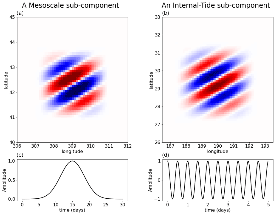
Figure 3 Illustration of one element of the basis for the mesoscale broadband signal (a) and for the internal tide narrowband signal (b). These upper panels show the element in space. For mesoscales, the represented element has a dominant wavelength and direction, but the ensemble of elements spans over all wavelengths and directions. For internal tides, the represented element has the dominant wavelength of the first baroclinic mode at the location considered (this is a mode-1 element) and a given direction, but the ensemble of elements also spans over both mode-1 and mode-2 wavelengths, and in all directions. The lower panels ((c, d)) show the element in time. For the mesoscale, the time extension is local as indicated by the Gaussian-like shape. For internal tides, the element persists in time with a sine modulation according to internal tide dynamics.

Then, if we note G_k=H_kΓ_k, where H_k is the observation operator from grid to observation space (trilinear interpolators), the observation vector y can be written as follows:

$$\begin{array}{}\text{(7)}& \mathbf{y}=\sum _{\mathbf{k}=\mathbf{1}}^{\mathbf{N}}{\mathbf{G}}_{\mathbf{k}}{\mathit{\eta }}_{\mathbf{k}}+\mathit{ϵ}=\mathbf{G}\mathit{\eta },\end{array}$$

where $\mathbf{G}=[{\mathbf{G}}_{\mathbf{0}},\mathrm{\dots },{\mathbf{G}}_{\mathbf{N}}]$ and $\mathit{\eta }=[{\mathit{\eta }}_{\mathbf{0}},\mathrm{\dots },{\mathit{\eta }}_{\mathbf{N}}]$, with N the number of components. The application of the OI formula to Eq. (7) gives

$$\begin{array}{}\text{(8)}& {\mathit{\eta }}^{\mathbf{a}}={\mathbf{QG}}^{\mathbf{T}}({\mathbf{GQG}}^{\mathbf{T}}+\mathbf{R}{)}^{-\mathbf{1}}\mathbf{y},\end{array}$$

where Q is the covariance matrix of the state vector η. Key assumptions are that the reduced basis Γ_k is orthogonal and that the components k are statistically independent. The first assumption can be satisfied by construction (diagonalizing the state covariances; see next two paragraph for practical implementation). The second assumption implies that there is no correlation between the different dynamics that will be considered for each component. In these conditions, Q has the following form:

$$\begin{array}{}\text{(9)}& \mathbf{Q}=\left[\begin{array}{ccc}{\mathbf{Q}}_{\mathbf{1}}& \mathrm{\dots }& \mathrm{0}\\ \mathrm{⋮}& \mathrm{\ddots }& \mathrm{⋮}\\ \mathrm{0}& \mathrm{\dots }& {\mathbf{Q}}_{\mathbf{N}},\end{array}\right]\end{array}$$

where Q_k are diagonal.

The equivalent covariance models are

$$\begin{array}{}\text{(10)}& {\mathbf{B}}_{\mathbf{k}}={\mathbf{\Gamma }}_{\mathbf{k}}{\mathbf{Q}}_{\mathbf{k}}{\mathbf{\Gamma }}_{\mathbf{k}}^{\mathbf{T}}.\end{array}$$

These covariance models will rely on the structure of elements in Γ and the variances chosen in Q for each of the elements, as detailed in the following. The mesoscales will constitute the first component, and the internal tides will be expressed as several components according the tidal frequencies and vertical modes.

3.2.1 The decomposition basis for mesoscales

The basis for mesoscales is the same as presented in Ubelmann et al., 2021, where the analytical formula of the ensemble of basis elements is given. Here, we only provide an illustration for comparison with the internal tide basis described in detail in the next section. The left panels of Fig. 3 show one of these elements for a particular wavenumber (of 150 km), with a typical time extension of 10 d. The ensemble of components characteristics and the diagonal terms of Q are designed to approach equivalent covariances of ocean mesoscale altimetry signals as explained in more details in Ubelmann et al., 2021. The database of SSH power density spectrum used to fill Q was built from the AltiKa along-track SSH anomalies The equivalent covariance model can be visualized if we plot, for a given point i of the space/time, the matrix product $\mathbf{\Gamma }[\mathbf{i},:]\mathbf{Q}\mathbf{\Gamma }[\mathbf{j},:{]}^{\mathbf{T}}$ as a function of j, hereafter called the representor. This is illustrated for j varying in space around i at the time of j (Fig. 4a) and at a 15 d time lag (Fig. 4c). The functions feature standard shapes of altimetry covariance models with a negative lobe as presented in (Traon et al., 1998). Note that the representer is not perfectly symmetric because geographical variations of the prescribed element variances (Q) introduce some inhomogeneity.

Figure 4 Illustration of the equivalent representer at a given location, for the mesoscale basis (a, c) and for the internal tide basis (d, b) as a function of space, for zero time lag (a, b) and for 15 d time lag (c, d).

3.2.2 The decomposition basis for internal tides

The basis for internal tides presents some similarities in the construction, but accounting for specific aspects of the internal tide dynamics, in particular the forcing frequency and the horizontal dispersion relation.

For the M2 and K1 forcing frequencies, the contribution of the first two vertical modes are considered, because they have a major contribution to SSH at the horizontal scales where altimetry observations are accurate (limited to 50–80 km along-track; Dufau et al., 2016), and also higher modes would certainly have more complex interactions. Here again, based on the assumption in the methodology, there is no statistical dependence between the modes so they are considered as independent components. For S2 and O1, only mode-1 is considered since their signal is weaker and mode-2 seemed challenging to resolve accurately.

For mode-1 (of any forcing frequency), we built a decomposition of plane waves following the dispersion relation between the time frequency w and spatial wavenumber k:

$$\begin{array}{}\text{(11)}& w^{\mathrm{2}}=k^{\mathrm{2}}{c}^{\mathrm{2}}+f^{\mathrm{2}},\end{array}$$

from which we can derive the phase velocity c_p (e.g., Zhao, 2019):

$$\begin{array}{}\text{(12)}& c_{\text{p}}={\displaystyle \frac{w}{\sqrt{w^{\mathrm{2}}-f^{\mathrm{2}}}}}c,\end{array}$$

where f is the Coriolis frequency and c the first baroclinic-mode phase speed. We specified regional variations for c following the Chelton et al., 1998 climatology, with values typically spanning between 1 m s⁻¹ in shallow or weakly stratified regions and 3.5 m s⁻¹ in the tropics and mid-latitude gyres. If lower values are obviously present in very shallow areas, these are not later defined in the climatology, and we did not consider the presence of internal tides in these areas (their wavelength would be shorter that the wavelength cutoff in the processing). The plane waves are defined as purely persistent in time, as illustrated in Fig. 3d, at exactly the forcing frequency considered for each component. However, in space, they are localized with a Hamming window at three spatial wavelengths (see Fig. 3b) to account for geographical variations due to topography (sources and sinks), inaccurate phase speed and any unconsidered physical interactions. The whole domain is paved with similar elements, and 12 angles for the plane wave directions. The number of angles must be large enough to cover all possibilities but not too large to avoid redundancies; its optimal value is related to the spatial extension of the plane wave (more precisely the Hamming window extension w.r.t. spatial wavelength). Finally, for each angle, two elements are defined (with $\mathit{\pi }/\mathrm{2}$ shift) to allow for the degree of freedom on the phase fit.

Using such a basis with constant terms for the Q diagonal matrix (equi-probability for each element), the representer of the first baroclinic mode of M2 $\mathbf{\Gamma }[\mathbf{i},:]\mathbf{Q}{\mathbf{\Gamma }}^{\mathbf{T}}$ for a given point of the grid at coordinates (190,30) is shown for zero time lag in Fig. 4b and 15 d time lag (plus half the tidal period) in Fig. 4d. The wavy pattern is clear on the representer shape, as opposed to mesoscales, since the waves are narrowband in space, by construction. There are also no attenuation in time (just phase fluctuations) as opposed to mesoscales, because the waves are infinite-narrowband by their construction.

For the second baroclinic mode where only M2 and K1 forcing frequencies are considered, the bases are constructed exactly in the same way, with a second vertical baroclinic phase speed approximated by $c_{\mathrm{2}}=c/\mathrm{2}$ . The phase speed from Eq. (12) is therefore divided by 0, resulting in spatial wavelengths twice as small as for the mode-1. The spatial Hamming windows are still scaled on three wavelengths. The total number of elements is therefore doubled in the meridional and zonal directions.

3.2.3 The inversion

Since the size of the parameter space is much smaller than the size of observation space, it is interesting to consider the Sherman–Woodbury transformation of Eq. (10), giving the equivalent following expression for η^a:

$$\begin{array}{}\text{(13)}& {\mathit{\eta }}^{\mathbf{a}}=({\mathbf{G}}^{\mathbf{T}}{\mathbf{R}}^{-\mathbf{1}}\mathbf{G}+{\mathbf{Q}}^{-\mathbf{1}}{)}^{-\mathbf{1}}{\mathbf{G}}^{\mathbf{T}}{\mathbf{R}}^{-\mathbf{1}}\mathbf{y}.\end{array}$$

The problem is solved on 15 by 15^∘ tiles separately, paving the whole globe with 2^∘ overlaps to allow smooth transitions on the final concatenation of the solution.

In each tile, the first step consists of filling the G matrix for mesoscales and internal tides following the basis decomposition described above, over the whole altimetry record. It consists, for each element, of an interpolation of the element value at each observation point. In practice, this interpolation is computed directly with the analytical expression of the element. For mesoscales, the number of elements (matrix column) is extremely large (10⁹ over 25 years and global domain) but the matrix is also extremely sparse. Indeed, as illustrated in Fig. 5a, very few observation points are included in a given element extension (local in time and space) which results in a manageable size. For internal tides, the number of elements is much smaller (10⁷) as the elements are local in space only but persist in time. The matrix is therefore more dense (sparse in space only), as illustrated in the right panel of Fig. 5b: the element contains more data (covering the 25 years of altimetry). The global size of the matrix is also manageable.

The second step is the resolution of Eq. (13), as explained in detail in Ubelmann et al., 2021, to converge toward the solution after typically 100 iterations with a conjugate-gradient method. Then, the third step is the projection of the solution in the grid space, formally Γη but in practice this is computed sequentially by adding each column of Γ (i.e., a given element) constructed online and multiplied by the ith component of η, bypassing the storage of Γ. The mesoscale solution is written at daily posting on a $\mathrm{1}/\mathrm{8}$^∘ grid in the zonal and meridional directions, while the internal tide solution is written on the same spatial grid but at a single date of reference (1 January 1990), at midnight and at midnight plus half the tidal frequency of the mode. Since the internal tide solution is coherent, these two fields are sufficient to reconstruct the solution at any time.

To overcome the large computational and storage demands of the G matrix, and in particular because the iterative matrix multiplications are much more efficient if G is stored in RAM, these three steps are performed on a supercomputer, occupying a total memory approaching 2 TB RAM shared by 200 threads. The G matrix is segmented, with appropriate communications at each computation of matrix products.

Finally, from the solutions on the overlapping 15 by 15^∘ boxes, a continuous global solution is computed by linearly interpolating the solution in the overlapping zones, with a weight ratio proportional to the boundary relative distances.

Figure 5 Illustration of the same elements as presented in Fig. 3 (from the mesoscale basis on the left and from the internal tide basis on the right), visualized in the observation space. The colored dots represent the non-zero values of a column of the G matrix.

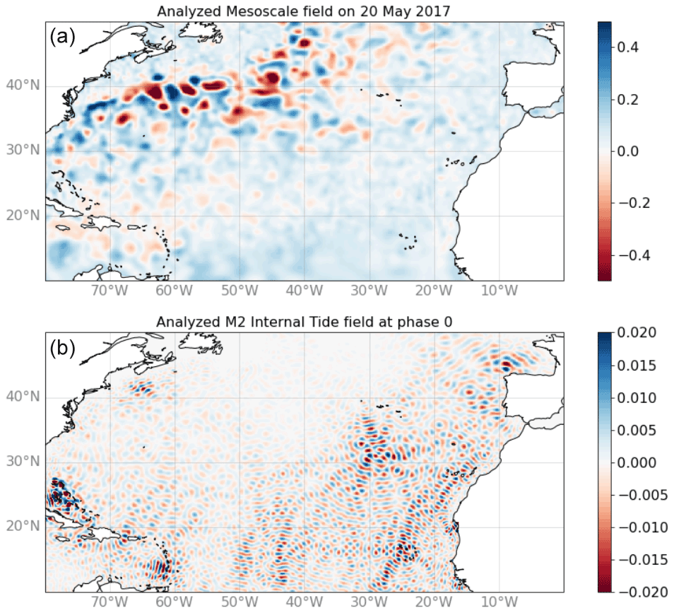
Figure 6 Snapshots of the reconstructed solutions in sea surface height (m) for 20 May 2017 at 00:00 UTC in the North Atlantic basin, for the mesoscale component (a) and for the internal tide component (b).

3.3 Results and validation

Both mesoscale and coherent internal tide estimations are provided by the inversion. The mesoscale solution, supposedly less affected by internal tide aliasing, is not analyzed in this paper, which is focused on the internal tide solution. The illustration in Fig. 6 shows the two mapped fields in the North Atlantic. The characteristics of each signal are very clear, with large mesoscale eddies on the top, dominating the signal variance, and the internal tides on the bottom, with clear generation sites showing up at the expected locations.

As mentioned above, the internal tides are resolved simultaneously but separately for each component (tidal frequencies and vertical modes). The illustration of all these components is particularly interesting in some regions where several components contribute, such as in the Philippine Sea, as shown in Fig. 7. As expected, the wavelengths for mode-2 are about twice as small as mode-1, and the wavelengths for K1 are twice as long as M2 since the time period is doubled. Note the K1 components dominates few areas in the 30^∘ S–30^∘ N tropical band. After verifying that no significant signal has projected in the K1 frequency beyond 30^∘ N and 30^∘ S, we run the final inversions without specifying the K1 components beyond 30^∘ N and 30^∘ S.

Figure 7 Snapshots of the reconstructed internal tide solutions in the Philippine Sea for M2 (a, b) and K1 (c, d), for the mode-1 contribution (a, c) and the mode-2 contribution (b, d).

In the following, we use the internal tide solution (written at the reference date) in a prediction mode assuming the stationary assumption persists over the period September 2017–December 2019, where we use independent altimetry data. These data also combine all satellite missions, and feature the same processing (barotropic tidal model in particular) as the main dataset used to compute the solution. To assess the quality of the reconstruction, we use a classical metric computing the variance difference before and after applying the prediction (e.g., Carrere et al., 2021), hereafter called variance reduction. When the latter is negative (less variance after the correction), we consider the correction to be efficient. In the following, the variance reduction is computed over integrated boxes or 2^∘ squared pixels.

Figure 8 (a–c) Snapshots of the M2 internal tide field north of the Hawaii ridge for three different experiment: in the first one (“MIOST-IT”, a) only the internal tide components have been considered in the inversion. In the second one (MIOST-MS then MIOST-IT, b) the internal tide mode inversion has been applied to observations for which the field from the mesoscale inversion had previously been removed. In the third one (MIOST-MSIT, c), the simultaneous inversion has been applied. (d) Variance of the solution (in blue) and explained variance after applying the solution as a correction to independent altimetry data (in green) for the three experiments mentioned above.

Figure 9 Same as Fig. 8 for the Gulf Stream area.

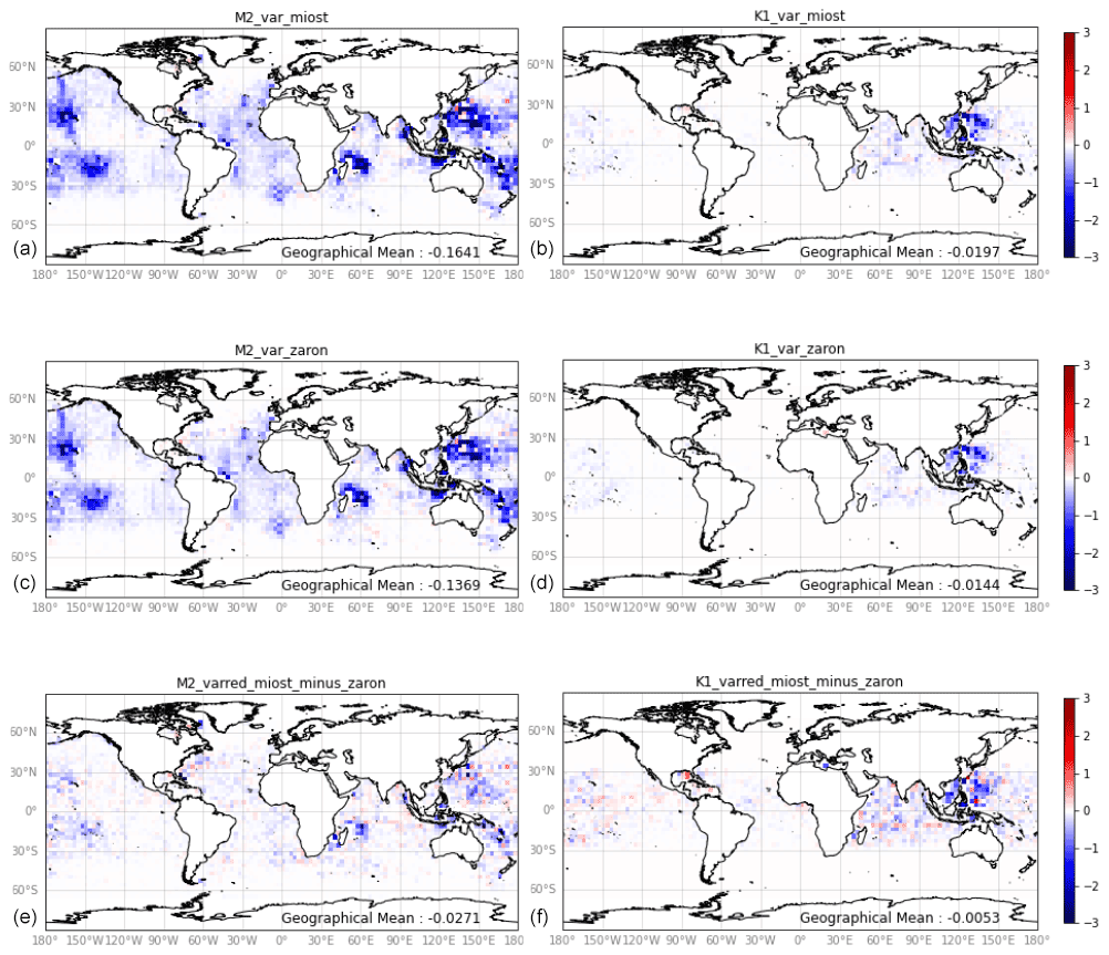
Figure 10 Difference of sea level anomaly variance (cm²) between along-track data of all satellites before and after applying the internal tide prediction, averaged over the independent period September 2017–December 2019. (a, b) With simultaneous MIOST reconstruction for the M2 component (a, c, e) and for the K1 component (b, d, f). (c, d) Same, with the Zaron, 2019 prediction model. (e, f) Difference between upper panels and middle panels.

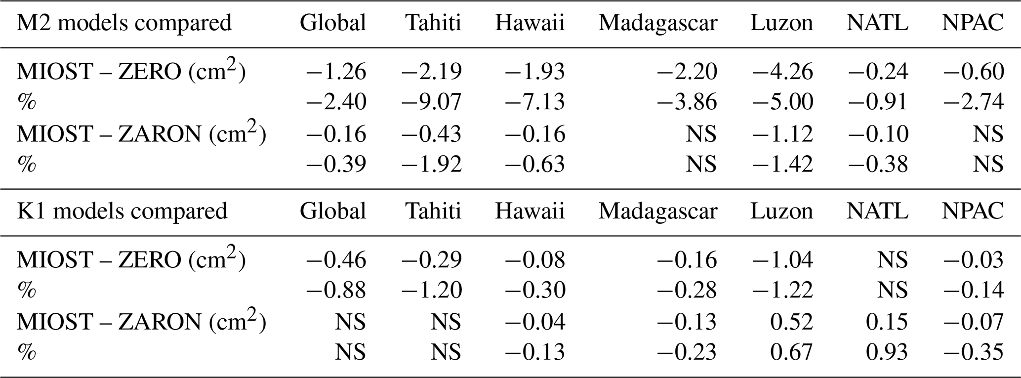
Table 1 Variance reduction for Cryosat-2 crossovers differences (cycles 96–124) when using the new MIOST internal tide solution and either a zero IT correction or the Zaron (2019) correction for M2 and K1 frequencies, in cm² and %. Values less than 0.1 % are not significant (NS).

3.3.1 The benefits of simultaneous estimations

Before analyzing the global solution, we propose to look at dedicated experiments where the estimation of internal tides is not simultaneous with mesoscales (only internal tide components are considered in the G matrix), a first experiment ignoring mesoscales, and a second considering mesoscales, but as a prior inverted separately. The results are shown in Figs. 8 and 9; the two experiments are labeled “MIOST-IT” and “MIOST-MS then MIOST-IT”, compared to the simultaneous experiment “MIOST-MSIT”. Figure 8 shows the Hawaii region, where mesoscale contamination is expected to be moderate for quite intense coherent internal tides. The effect of the simultaneous inversion is notable with a reduction of variance after applying the correction (green bars), exceeding the first two experiments. As expected, the variance of the solution (blue bars) is higher in the first experiment (mesoscale contamination) while in the second experiment, the variance is much lower, probably because the prior mesoscale field contained aliased internal tides, therefore reducing the apparent internal tides. Figure 8 shows the Gulf Stream region with intense mesoscales and potentially low coherent internal tides. Here, the effect of simultaneous inversion is even stronger. In absence of mesoscale consideration, some internal tides are estimated in the Gulf Stream (as suggested by the strong positive blue bar for MIOST-IT in the figure), but the reduction variance is negative (as suggested by the negative green bar), meaning that the estimations feature more errors than the actual signal. This is also clearly the effect of mesoscale aliasing. Note the importance of using independent data over an independent period out of the analysis window: if we used the data during the analysis, the variance reduction would be positive by construction. In the second experiment, the same effect as in the Hawaii case is observed, and amplified: the internal tides are very attenuated because the prior mesoscale estimates are contaminated in phase with the internal tides during the period of analysis. Finally, the simultaneous inversion seems to do quite a good job in the Gulf Stream, resolving some internal tides in the continental slope area, although probably attenuated since the variance reduction exceeds the signal variance (the Q matrices for mesoscales and internal tides may need to be adjusted to tolerate somewhat more internal tides).

3.3.2 Global validation

The main simultaneous inversion experiment that featured the expected mitigation of aliasing issues over independent or sequential estimations is now validated globally and compared with an existing internal tide solution from Zaron (2019). Here again, we propose to evaluate the reduction of signal variance after applying the solution as a correction to the independent altimetry observations mentioned above. The global SLA variance reduction has been computed over 2^∘ by 2^∘ cells over the September 2017–December 2018 multi-satellite altimetry data, a period during which none of the estimations have seen the data. The results are shown in Fig. 10, for the two major components M2 and K1 (including first and second baroclinic modes). First, there are no regions (except a few red pixels) where the estimation fails: everywhere the variance reduction is either positive (blue meaning negative difference, i.e., positive reduction) or absent. It is very positive in the expected sites of internal tide generation where internal tides are supposedly coherent. The equatorial regions, known to feature phase-varying internal tides because of strong currents, have indeed no significant variance reduction (nor signal, not shown). The comparison with the Zaron (2019) model is at first order very similar, which we consider as a success since the approach was new and could have led to unexpected issues. Then, a closer look at the differences between the two estimates (see Fig. 10e and f) would suggest that the variance reduction is, on global average, slightly higher in this study, especially in the regions of high internal tide energy. Also, it might be of interest to note that the wave train resolved north of the Gulf Stream (see Fig. 8c) shows up with a few blue pixels in Fig. 10e, whereas the Zaron model does not provide a signal here (flagged region). Finally, there are still some areas where the Zaron (2019) features more variance reduction, for instance with K1 in the Eastern Tropical Pacific.

Another interesting diagnostic is the variance reduction at ground-track crossover differences, because it naturally suppresses some of the large timescale variability of mesoscales, but keeps the energy of internal tides. The diagnostic was run and integrated over different region, as detailed in Carrere et al. (2021), but here applied to MIOST and Zaron (HRET) with the Cryosat-2 data. The integrated variance reductions computed for Cryosat-2 mission have been integrated over the main regions of intense internal tide, and for M2 and K1 components available in both models, as shown in Table 1. The results are indeed very close between the two models, and would confirm a slight advantage of the simultaneous inversion presented in this study in terms of variance reduction.

4 Conclusions

The simultaneous inversion of mesoscale variability and internal tide signatures on sea surface height has been successfully implemented globally, constituting in particular an additional empirical internal tide solution to the existing ones. It was designed to minimize aliasing effects, by accounting for the statistics of mesoscales and internal tides in a global linear analysis framework.

The computation of uncertainties could be an interesting next step. Indeed, it would be possible to provide estimations of errors, with respect to the covariance model prescribed through the mode decompositions for mesoscales and internal tides (first given in the parameter space, but then projectable in physical space). This would be a future improvement, considering that the successful quantitative validation with independent data was the most important milestone for this new internal tide model.

The methodology applied in this study could also be extended to internal tides with phases varying seasonally, as already implemented in Zhao (2021). Practically, we would introduce additional components that could be built with the same plane wave basis, modulated with sines and cosines at a 1-year frequency. Also, with the prospect of future wide-swath altimetry providing a larger volume of data, the incoherent internal tides could also be tackled with time-finite modulation of the plane waves. This is obviously a challenge that will not be met everywhere, in particular where mesoscale fields dominate, but we hope that in some regions, some part of the incoherent waves can be captured.