Passive tracer advection in the equatorial Pacific region: statistics, correlations and a model of fractional Brownian motion

Evaluating passive tracer advection is a common tool to study flow structures, particularly Lagrangian trajectories ranging from molecular scales up to the atmosphere and oceans. Here we report on numerical experiments in the region of the tropical Pacific (20^∘ S–20^∘ N), where 6600 tracer parcels are advected from a regular initial configuration (along a meridional line at 110^∘ W between 15^∘ S and 15^∘ N) during periods of 1 year for 25 years altogether. We exploit AVISO surface flow fields and solve the kinematic equation for passive tracer movement in the 2D advection tests. We demonstrate that the strength of the advection defined by mean monthly westward displacements of the tracer clouds exhibit surprisingly large inter- and intra-annular variabilities. Furthermore, an analysis of cross-correlations between advection strength and the El-Niño and Southern Oscillation (SOI) indices reveal a significant anticorrelation between advection intensity and ONI (the Oceanic Niño Index) and a weaker positive correlation with SOI, both with a time lag of about 3 months (the two indices are strongly anticorrelated near real time). The statistical properties of advection (time-dependent mean squared displacement and first passage time distribution) suggest that the westward-moving tracers can be mapped into a simple 1D stochastic process, namely fractional Brownian motion. We fit the model parameters and show by numerical simulations of the fractional Brownian motion model that it is able to reproduce the observed statistical properties of the tracers' trajectories well. We argue that a traditional explanation based on the superposition of ballistic drift and a diffusion term yields different statistics and is incompatible with our observations.

1 Introduction

Studies of regular or chaotic advection of various tracer particles are a growing area of research thanks to measurements with increasing sampling densities and numerical models with ever-better resolutions (Aref et al., 2017). Phenomena related to advection cover a very wide range from molecular scales to geophysical flow fields in the atmosphere and oceans. The starting point of the subject is certainly the simplest case: passive tracer advection (Aref, 1984; Ottino, 1990). In a fluid treated as a continuum, one can conceptually mark a particle (a microscopic parcel) that moves passively with flow velocity v from the initial position r(0)=r₀ and obeys the simple kinematic equation

$$\begin{array}{}\text{(1)}& {\displaystyle \frac{\mathrm{d}r\left(t\right)}{\mathrm{d}t}}=\mathit{v}\left(r\left(t\right)\right).\end{array}$$

The resulting Lagrangian trajectories r(t) permit an insight into the details of the flow structures and mixing. A fundamental finding is that very simple time-periodic flow fields may advect tracers chaotically, as indicated by an exponential divergence from their close initial positions. In most cases, it is possible to reconstruct invariant sets of a fractal nature in the phase space related to chaotic advection (see, e.g., Péntek et al., 1995; Cartwright et al., 1999; Tél et al., 2000; Speetjens et al., 2021). Recent important applications are connected to the exploration of Lagrangian coherent structures (Haller, 2015; Hadjighasem et al., 2017; Haller et al., 2018; Beron-Vera et al., 2018; Callies, 2021; Haller et al., 2021), mostly in the context of ocean flows.

Studies of advection and material transport in the oceans are growing in importance, partly because of catastrophes such as the Deepwater Horizon explosion (Gulf of Mexico, 2010; see, e.g., Olascoaga and Haller (2012)) or the nuclear disaster in Fukushima (Japan, 2011; see, e.g., Prants et al. (2017). Besides these extreme events, “traditional” interest has been growing in the transport of plankton (Károlyi et al., 2000; Huhn et al., 2012; Hernández-Carrasco et al., 2020; Villa Martín et al., 2020), heat (Webb, 2018; Adams et al., 2000; Ruggieri et al., 2020), salt (Delcroix and Picaut, 1998; Sanchez-Rios et al., 2020; Paul et al., 2021), oxygen (Rudnickas et al., 2019; Audrey et al., 2020) and other chemicals (Behrens et al., 2020; Jones et al., 2020). Another classical list of works aim to determine mixing rates by determining surface eddy diffusivities (see, e.g., Abernathey and Marshall, 2013, and references therein).

When considering ocean surface current systems, the equatorial Pacific is certainly a key region from many respects (see, e.g., Reverdin et al., 1994; Yu and McPhaden, 1999; Grodsky and Carton, 2001; Chepurin and Carton, 2002; Capotondi et al., 2005; Izumo, 2005; Kessler, 2006; Bulgin et al., 2020; Wang et al., 2020; Power et al., 2021). The El Niño–Southern Oscillation (ENSO) has a near-global impact on weather, agricultural yields, air quality and even landslides (Grove, 1998; Collins et al., 2010; Chang et al., 2016; Luo et al., 2018; Timmermann et al., 2018; Emberson et al., 2021; Power et al., 2021). Based on recent observations (mostly Argo buoys) and high-resolution numerical ocean models, it has become clear that the tropical Pacific region has a complicated 3D structure. Besides the surface currents, determining features are the equatorial upwelling zone (resulting in poleward Ekman transport), the equatorial undercurrent (an energetic eastward flow at the depth of the pycnocline ∼ 50–200 m), and the shallow meridional overturning circulation both north and south of the Equator.

Here we focus on the tropical Pacific region and compute Lagrangian trajectories by a passive tracer advection approach using Eq. (1). The velocity fields are obtained from AVISO altimetry data (Aviso, 2022; Taburet et al., 2019), which has a higher spatial resolution ($\mathrm{0.25}{}^{\circ }\times \mathrm{0.25}{}^{\circ }$) than global ocean numerical models (usually $\mathrm{1}{}^{\circ }\times \mathrm{1}{}^{\circ }$), whereas the resolution in regional ocean models can be as fine as 3–9 km (Nefzi et al., 2014). We will demonstrate that the overall behavior of tracers is an anomalous diffusion process that is slower than a pure drift but faster than simple diffusion. The novel observation here is that the Hurst exponent of this anomalous diffusion process is a constant value for a large range of spatial (from 1 to 5000 km) and temporal (from 2 to 365 d) scales. This means that the collective effect of the spatial and temporal fluctuations of the velocity field that advects the particles has some self-similar structure, which gives rise to a rather uniform time evolution on average over several years. Instead of a constant Hurst exponent over such large ranges of spatial and temporal scales, one might expect some crossover effects, e.g., from (anomalous) diffusion on small scales to ballistic, drift-dominated transport on larger scales. The absence of such crossover effects shows that the irregularities of the velocity fields in space and time do not average out, even at large scales, and might reflect some kind of scale invariance of the 2D turbulent motion of these hydrodynamic flows. This provides insight into the statistics of oceanic turbulence and might be of fundamental physical interest.

An alternative description would be a model with an explicit ballistic drift term plus normal diffusion. The drift term would then describe the time dependence of the mean value of the zonal particle positions, and the normal diffusion term would explain why the variance of this distribution grows over time. Our analysis clearly shows that the statistical properties of such a quite plausible model are incompatible with the observations based on numerical tracer advection.

In the next section, we summarize the data sources and methodologies of the statistical analysis. The section “Results and discussion” gives an overview of the large variability we obtained in the strength of the advection and of cross-correlation properties with the El Niño and composite Southern Oscillation indices. The trajectories indicate a strong westward drift and relatively weak dispersion in the meridional directions, which provides a mapping to a one-dimensional stochastic random walk model. Statistical analysis of the mean squared displacement in the zonal direction and of first passage times suggests that an appropriate model of this kind is fractional Brownian motion (fBm) with some small, deterministic, westward drift. We fit the parameters of this model and validate it using numerical simulations. We demonstrate that a deterministic drift term provides negligible improvement, so we end up with a two-parameter fBm model.

2 Data and methods

Geostrophic surface velocity fields were obtained from the AVISO data bank (Aviso, 2022; Taburet et al., 2019). Geostrophic balance does not hold at the Equator, but the altimetry data can still be used to infer velocities there, albeit with somewhat lower accuracy. The AVISO data-processing algorithm implemented the method of Lagerloef et al. (1999) between the latitudes $\pm \mathrm{5}{}^{\circ }$ (Aviso, 2022; Taburet et al., 2019). We used the direct zonal and meridional velocity components (u_gos and v_gos, in units of m s⁻¹). The spatial resolution of daily global records is 0.25${}^{\circ }\times \mathrm{0.25}{}^{\circ }$ (1440 × 720 grid cells). Land areas are masked. The temporal resolution is 1 d between the period 1 January 1993 and 23 October 2018; however, we cut out the last truncated year to allow the proper comparison of annual results. Offline passive tracer advection was estimated by bilinear interpolation of velocity values and by solving Eq. (1) using a fourth-order Runge–Kutta method with a time step of 5 min. The positions of advected parcels were recorded every 12 h throughout a given year (365 d). On 1 January each year, 6600 tracers were started from a meridional line at longitude 110^∘ W and between latitudes 15^∘ S and 15^∘ N (with approximately 500 m of spacing). All calculations were performed using the package Ocean Parcels (Lange and van Sebille, 2017; Delandmeter and van Sebille, 2019) in a Python environment (version 3.6) with the standard Numpy (Harris et al., 2020) and Scipy (Virtanen et al., 2020) libraries. Maps were drawn using the Cartopy module (Met Office, 2010–2015). As representative examples, Fig. 1 illustrates two consecutive years, 1997 and 1998. 1997 was a very strong El Niño year, and Fig. 1a clearly demonstrates the well-known effect of weakened (easterly) trade winds in such years.

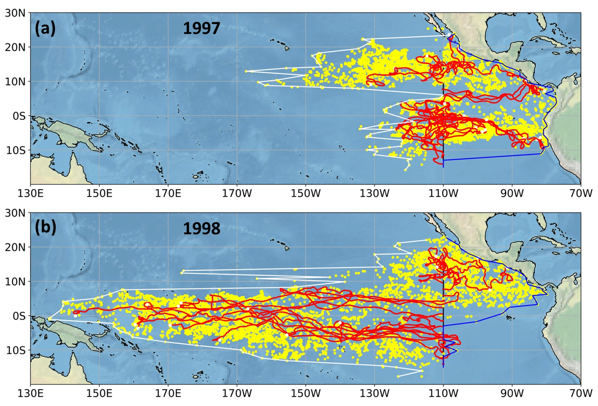
Figure 1 The final positions of passively advected parcels (yellow dots) after 365 d. Start date: (a) 1 January 1997 (a particularly strong El Niño year) and (b) 1 January 1998. The initial positions of the 6600 tracers were along a meridional line at longitude 110^∘ W and between latitudes 15^∘ S–15^∘ N (black vertical line on the maps). The white/blue lines indicate the western/eastern envelopes of the tracer clouds after 1 year of advection, while red lines exhibit representative trajectories. The flow fields are from the AVISO data bank (Aviso, 2022; Taburet et al., 2019).

Similar numerical experiments are reported in Webb (2018), where hot parcels (T>27 ^∘C) are advected in two years (1981 and 1982) from 24 June to the end of the year from an initial meridional line in the middle of Pacific, north of the Equator (see Figs. 26 and 27 in Webb, 2018). The high variability of the North Equatorial Counter Current (NECC) is nicely demonstrated.

We have no access to the vertical velocity field, and no model for the advection of particles in 3D with the ocean surface as a boundary. Clearly, real transport is not restricted to the topmost horizontal layer of the ocean, but it is a useful approximation and a standard approach to ignore the third dimension in such transport studies. We assume that our numerically advected tracer paths are sufficiently realistic compared to, e.g., floaters released to the ocean. Note, however, that a direct comparison of our analysis with trajectories of drifting surface buoys or satellite altimetry is not straightforward because our initial configuration (parcels arranged along a meridional line) is rather specific for each year. Furthermore, surface buoys are directly affected by surface wind shear, so their drifts do not always reflect the displacements of underlying water parcels (Reverdin et al., 1994; Grodsky et al., 2011).

Based on the advection data for each year, we adopted two definitions of an “advection index” (AdI) to characterize the westward drift strength. A rather large fraction of parcels travel to the east from the initial position and remain trapped in the eastern equatorial Pacific (see Fig. 1). However, in this work, we do not consider their complicated behavior, but rather focus on the westward-moving tracers. The monthly advection indices AdI₁ and AdI₂ are defined as the ensemble mean values of two metrics: (1) the zonal distance and (2) the total trajectory length (meridional drift components are included) from the positions at the end of the previous month. We will see that there is no difference between the values of both standardized indices, demonstrating that westward drift completely dominates. On an absolute distance scale, AdI₁ is systematically lower than AdI₂, as expected, but the difference is negligible.

In order to connect the AdI with well-known large-scale climate patterns, we determined cross-correlations with two standard indices, the Southern Oscillation Index (SOI) and the Oceanic Niño Index (ONI). (Actually, we also checked other distant index values, such as Arctic Oscillations and Antarctic Oscillations, but we only obtained meaningful correlations with the two “local” diagnostic quantities.) The standardized SOI is obtained from the monthly or seasonal differences in air pressure between Tahiti and Darwin, Australia (Trenberth and the Atmospheric Research Staff, 2020). ONI is almost the same as the “traditional” Niño 3.4 index, being based on mean sea surface temperature anomalies over the area 5^∘ S–5^∘ N, 170–120^∘W. ONI is the operational definition used by NOAA to define an El Niño or La Niña event.

Normalized cross-correlations between two signals x(t) and y(t) are determined as usual:

$$\begin{array}{}\text{(2)}& X\left(\mathit{\tau }\right)={\displaystyle \frac{\langle \left[x\right(t)-\stackrel{\mathrm{‾}}{x}]\left[y\right(t+\mathit{\tau })-\stackrel{\mathrm{‾}}{y}]\rangle }{{\mathit{\sigma }}_x{\mathit{\sigma }}_y}},\end{array}$$

where the time lag τ represents a temporal shift of ±τ months between the two time series, an overbar denotes a temporal mean and σ is the standard deviation of the given time series. Note that according to the above definition (realized in the scipy.signal.correlate() routine), the second signal y(t) moves along the time axis in both positive and negative directions with respect to x(t). Thus, a positive lag correlation means that y(t) leads x(t), and vice versa.

The confidence interval (at a level of 99 %) for cross-correlations is obtained in the following way. It is well known that the presence of serial or higher-order autocorrelations in x(t) and y(t) can yield spurious cross-correlations (e.g., Zwiers, 1990; Ebisuzaki, 1997; Massah and Kantz, 2016). Following the proposal in, e.g., Ebisuzaki (1997), we computed 10 000 surrogate data sets $\mathit{\left\{}{x}_i^{\prime }\right(t\left)\mathit{\right\}}$ for x(t) by the iterative amplitude adjusted Fourier transform (IAAFT) method (Kantz and Schreiber, 1997; Hegger et al., 1999; Schreiber and Schmitz, 2000; Lancaster et al., 2018). Such surrogates reproduce the amplitude distribution and power spectrum of the source record x(t). We used 100 iterations in a given run to build the ensemble $\mathit{\left\{}{x}_i^{\prime }\right(t\left)\mathit{\right\}}$. Then we calculated X(τ) by Eq. (2) for each pair [$x_i^{\prime }\left(t\right),y\left(t\right)$] of signals. After arranging cross-correlation values for each time lag τ in increasing order, the 99 % confidence interval was obtained from the percentile range [0.05, 99.5] (i.e., we dropped the lowest 50 and highest 50 values from an ordered test ensemble of 10 000 members). Note that the surrogate data method is a modification of classical bootstrapping, where both the marginal distribution of the data and their serial correlations are conserved when creating otherwise random samples.

The statistical analysis of advection is based on two standard measures, the first passage time (FPT) (Metzler et al., 2014b) and the mean square displacement (MSD) (Jánosi et al., 2010; Haszpra et al., 2012; Kepten et al., 2015). Both measures have a transparent definition: in our setup, the FPT is the time when a given longitude is crossed by a parcel and the MSD is calculated as the time evolution of the squared distances from the initial location. In the second case, a refined statistics is also adopted by computing the time-averaged mean square displacement (TAMSD) (Lubelski et al., 2008; Kepten et al., 2015; Sikora et al., 2017; Maraj et al., 2021). In this case, the whole trajectory of a parcel is evaluated by introducing the time window parameter w, which changes from 12 h to 315 d (2 × 315 time steps in the record). This time window moves along the trajectory step by step, and a temporal mean is computed for the squared displacements in window w. This procedure is computationally rather demanding, but it smooths out, e.g., seasonal and intraseasonal fluctuations.

3 Results and discussion

3.1 Advection index

As discussed in the previous section, in order to determine the strength and variability of the advection, we use two (monthly) advection indices AdI₁ and AdI₂. The subsequent analysis distinguishes two subsets of tracers based entirely on their initial positions: parcels north/south of the geographic Equator are separated into northern/southern sections because it is not clear a priori whether these two advection processes have the same statistical properties. The reason for this simplistic subset definition is that hemispherical surface winds and surface ocean currents in a given short period are determined not by the geographic zero latitude but rather by the thermal or heat equator, which actually has a strong coincidence with the Intertropical Convergence Zone (ITCZ) (Amador et al., 2006a; Kessler, 2006b). The location of the ITCZ or, equivalently, the thermal equator is not simply zonal, and has an annual cycle that follows the changes in the incoming shortwave solar radiation flux. The mean position of it is around 5^∘ N because the ice mass of the Antarctic and the lower fraction of land in the Southern Hemisphere result in a lower mean temperature south of the geographic Equator. This mean location is clearly visualized by maps of annual precipitation in the region (see, e.g., Fig. 7. in Amador et al., 2006a) or by the long-term mean position of the NECC (see, e.g., Fig. 1 in (Hsin and Qiu, 2012) or Figs. 1 and 3 in (Wijaya and Hisaki, 2021)). The dynamic relocation of ITCZ over the year has the consequence that trade winds and ocean surface currents also change, so advected parcel trajectories often cross the geographic Equator and the mean thermal equator. There are some years (usually with weaker advection strengths) when the separation of the northern- and southern-drifting parcels is clear, as is the presence of the NECC (see Fig. 1a). In other years (usually those with strong advection), such separation is not so clear (see Fig. 1b).

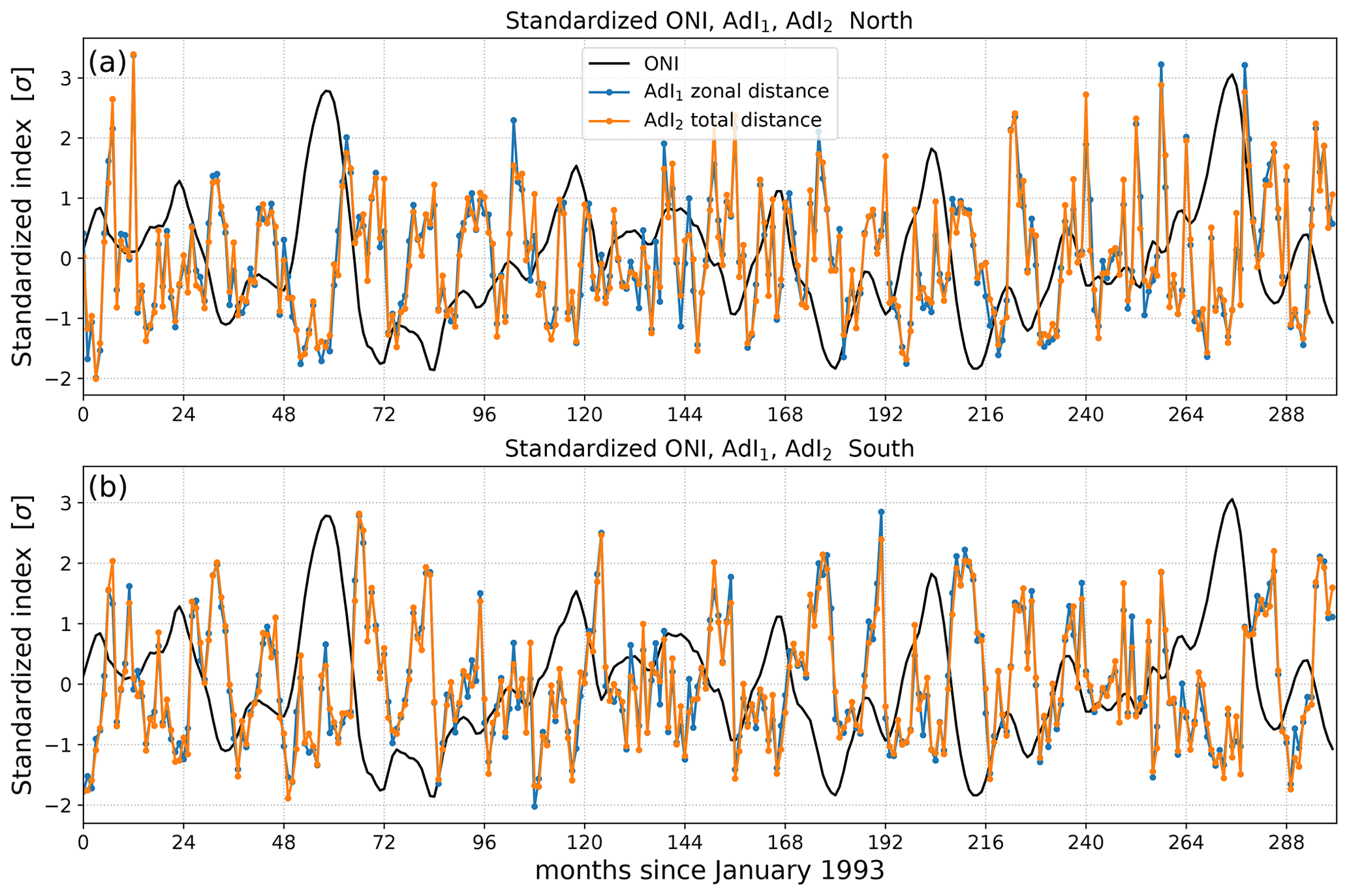
Figure 2 Standardized advection indices AdI₁ and AdI₂ determined as ensemble averages of the monthly westward displacements. The first is based on the monthly zonal distance from the position at the end of the previous month; the second is the total trajectory length in a month (meridional components are also taken into account). For a comparison of variabilities, the ONI (Oceanic Niño Index) is also plotted as black lines. (a) northern section; (b) southern section.

We note here that the instantaneous (daily) location of the ITCZ line is a delicate question, which is why the ITCZ is usually illustrated by long-term mean values in the literature. We could not figure out an adequate method to separate parcels on the two sides of the ever-changing ITCZ line.

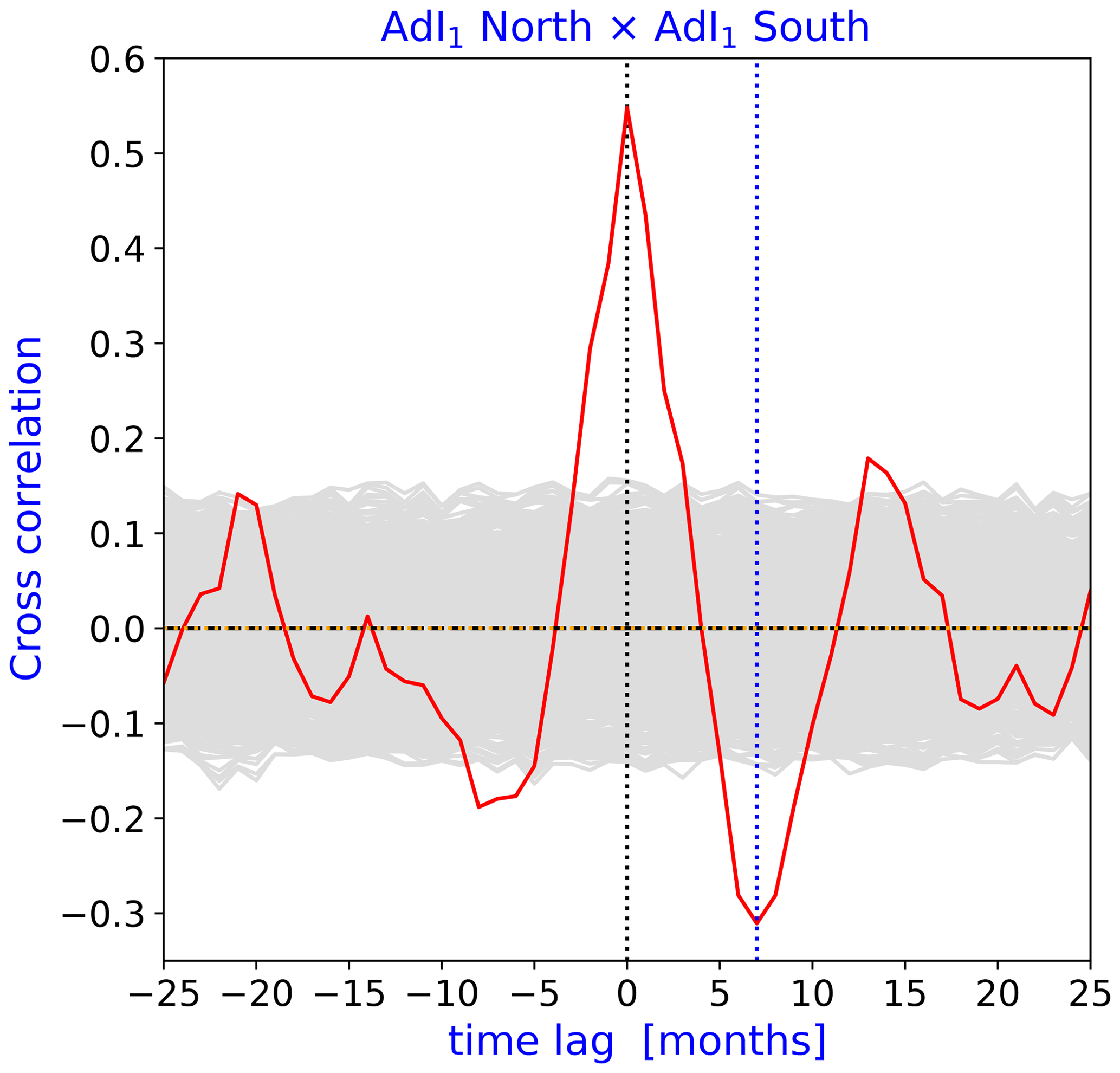
Figure 3 Cross-correlation between the monthly advection index AdI₁ for the northern and southern subsets of advected parcels (red). Dashed blue/black line indicates the time lag at which the cross-correlation is at its absolute minimum $/$ maximum. The gray band indicates the 99 % confidence interval, as described in Sect. 2.

Figure 2 exhibits the advection indices together with the ONI (Oceanic Niño Index). The definitions of AdI₁ and AdI₂ result in almost identical standardized monthly mean values, indicating that pure zonal drift dominates for westward-moving parcels. (Standardization is obtained in the usual way: by removing long-term mean values and normalizing by the standard deviation.) A simple visual inspection is enough to detect substantial differences between the northern and southern subset of parcels (compare Fig. 2a and b). Indeed, when we determine cross-correlations [Eq. (2)] for the northern and southern advection indices, there are some remarkable features; see Fig. 3.

The first remarkable aspect of Fig. 3 is that the real-time positive correlation is rather moderate (X(0)=0.55), so the northern and southern Pacific currents are not strongly coupled. The second aspect is the presence of a weaker but statistically significant (at the 99 % level) anticorrelation with a time lag of 7 months ($X(\mathit{\tau }=\mathrm{7})=-\mathrm{0.31}$). Similar anticorrelation is usually explained by the fact that the seasons in one hemisphere appear in counterphase with the seasons in the other hemisphere. For this reason, practically every climatology that considers monthly mean values and anomalies automatically assumes a time lag of 6 months. Note that in Fig. 3, neither the location of the minimum nor those of the faint local maxima of positive correlations precisely follow the periodicity of 1 calendar year. While seasonality in the weather is not essential in the tropical band, the annual cycle of the location of the thermal equator follows the changes in insolation.

The observed relatively weak real-time positive correlation and the statistical feature of the phase shift of ∼7 months between the northern and southern tracer subsets suggested to us that all subsequent statistical tests should be performed separately. We will illustrate that the results are very similar but not identical.

3.2 Cross-correlations with the climate indicators ONI and SOI

Figures 4 and 5 illustrate the cross-correlations Eq. (2) between the two monthly climate indicators ONI and SOI and the advection index AdI₁ separately for the two hemispheres or the joint AdI₁ incorporating the monthly zonal distances traveled by all the westward-drifting parcels. For the ONI, the main feature is an absolute negative minimum at a time lag of 3 months. SOI has a positive correlation at the same time lag. Furthermore, a weaker but significant positive correlation with ONI and a negative correlation with SOI (at least in the Southern tracer subset) appear with a time lag of −7 months. All these are fully consistent with the well-known strong real-time anticorrelation between ONI and SOI.

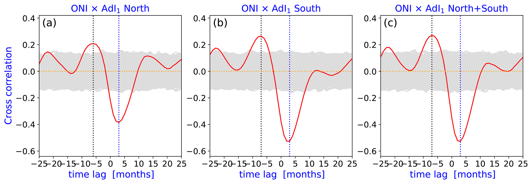
Figure 4 Cross-correlation between ONI and the monthly advection index AdI₁ for the northern and southern subsets of advected parcels (red). Dashed blue/black line indicates the time lag at which the cross-correlation is at its absolute minimum $/$ maximum. The gray band indicates the 99 % confidence interval, as described in Sect. 2. (a) AdI₁ for the northern subset (see Fig. 2a). (b) AdI₁ for the southern subset (see Fig. 2b). (c) Cross-correlation between ONI and the monthly advection index AdI₁ for all the westward-moving parcels. The strongest anticorrelation occurs at +3 months in each case, meaning that the advection strength AdI₁ leads ONI: a marked weakening of advection is followed by a warming SST signal with a delay of 3 months, and vice versa.)

Figure 5 Cross-correlation between SOI and the monthly advection index AdI₁ for the northern and southern subsets of advected parcels (red). Dashed blue/black line indicates the time lag at which the cross-correlation is at its absolute minimum/maximum. The gray band indicates the 99 % confidence interval, as described in Sect. 2. (a) AdI₁ for the northern subset (see Fig. 2a). (b) AdI₁ for the southern subset (see Fig. 2b). (c) Cross-correlation between SOI and the joint monthly advection index AdI₁ for all the westward-moving parcels. The strongest correlation occurs at +3 months in each case, meaning that the advection strength AdI₁ leads SOI: a strengthening of advection is followed by an increasing pressure anomaly (above-normal air pressure at Tahiti and below-normal air pressure at Darwin, Australia) with a delay of 3 months, and vice versa.

Since the two quasiperiodic oscillations ONI and SOI are strongly anticorrelated in near real time, the advection index behaves as expected. The interpretation for a time lag of 3 months is not so trivial. Obviously, correlation is not equivalent to a causal link; the only information that can be extracted with high confidence is the temporal sequence of events. The time lag of 3 months suggests that when the ONI index rises (the Niño 3.4 area warms up), and the SOI index decreases (the air pressure anomaly between Tahiti and Darwin drops) in parallel, the advection strength decreases significantly 3 months later. Analogous behavior occurs in the opposite direction: when ONI drops and SOI increases, the westward advection is accelerated 3 months earlier. This rather long delay is somewhat perplexing, because it is known that the characteristic response time of the ocean surface currents to zonal wind bursts (lasting typically 5–15 d) is a few days at most. This is observed around the Antarctic Circumpolar Current (Webb and de Cuevas, 2007) and at the western sector of the equatorial Pacific (McPhaden et al., 1992; Delcroix et al., 1993; Richardson et al., 1999). It is well known that during an El Niño event, the prevailing trade winds and the surface westward currents suffer from a temporary reversal in the western part of the Pacific basin. Our analysis suggests that this reversal, blocking advection, propagates toward the eastern basin for about 3 months.

We have already mentioned that the tropical Pacific currents have a rather well-known complex 3D structure. Capotondi et al. (2005) and Izumo (2005) determined lag correlations between various branches (equatorial undercurrent and shallow meridional overturning cells) and the spatial mean of the sea surface temperature over the Nino3.5 area. High-resolution 3D ocean models have found significant cross-correlations with various time lags on the scale of months. Izumo (2005) observed anticorrelations between the SST signal and the surface divergence (poleward Ekman transport) with a lag of 5.5 months, equatorial upwelling (τ=5 months), equatorial undercurrent (τ=3 months) and pycnocline convergence (τ=0.5 months), suggesting that the changes in the 3D current structure lead the appearance of an El Niño signal. An interesting result noted by Capotondi et al. (2005) is that equatorward mass convergence along the pycnocline and equatorial upwelling are related to the SST. The strongest correlation is found when SST leads the meridional mass convergence by 2 months, a result that seems to disagree with the view that changes in the strength of the subtropical-tropical cells (STCs) cause the SST changes. Since we do not have access to the 3D flow structure, we cannot relate our finding (that SST lags behind advection strength changes by ∼3 months at the very surface) to the results of Capotondi et al. (2005). They notice, however, that “phase relationships among the different STC components can be largely affected by the zonal averaging procedure because of the continually evolving nature of the STCs.”

3.3 Statistical properties of westward advection

From Fig. 1, it is evident that the tracers exhibit highly complex motion that contains many aspects of stochasticity. Therefore, it is natural to analyze the tracer trajectories in terms of a diffusive process. We do so by focusing on three essential characteristics that allow us to better understand which stochastic process is best suited to explaining the observed phenomena.

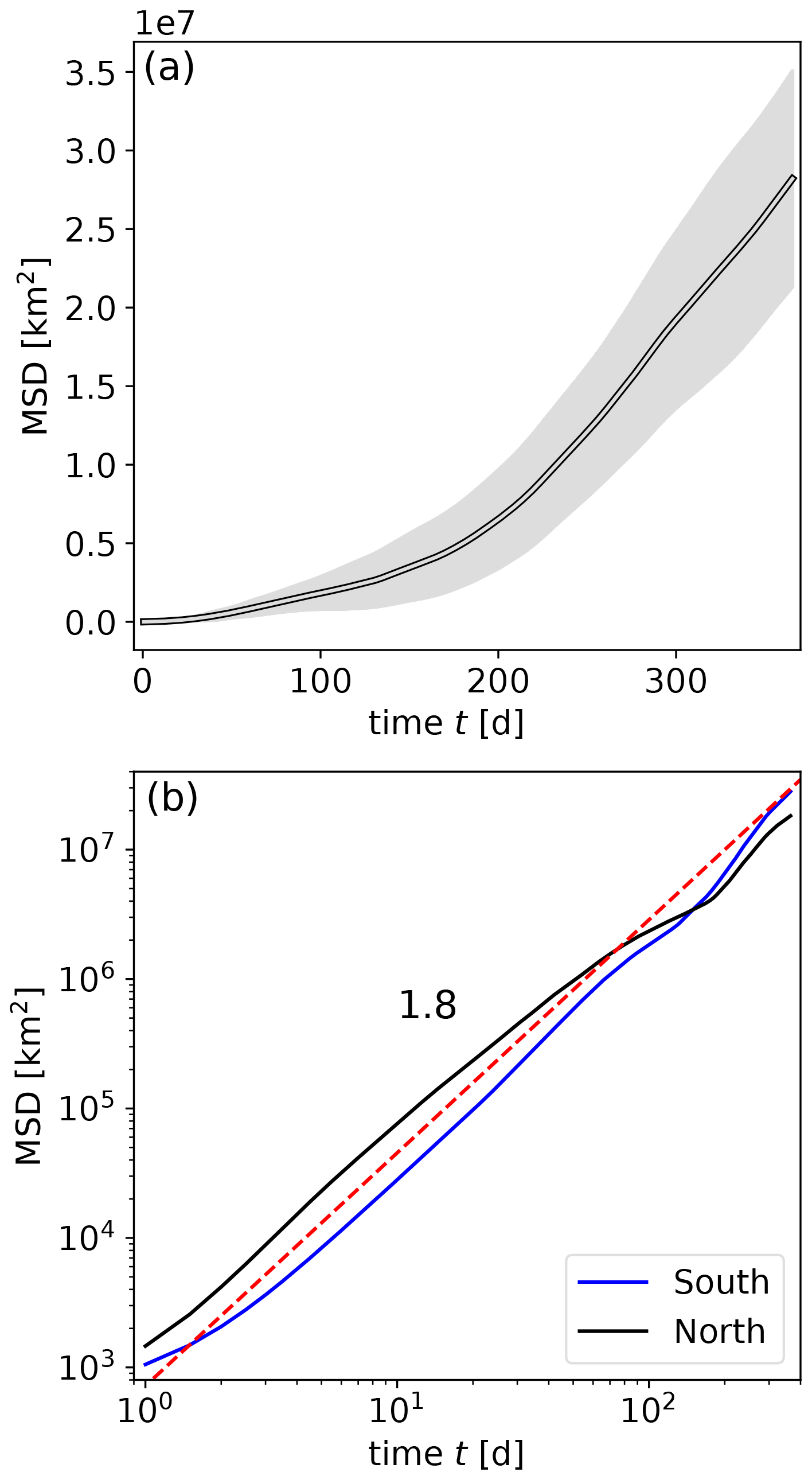
Figure 6 Mean squared displacement (MSD) for the advected parcels in units of km². The spherical geometry was fully taken into account when calculating distances from the initial positions. (a) MSD for the northern subset (lin-lin plot). The error band reflects the standard deviation obtained from year-by-year statistics. (b) MSDs for both the northern (black) and southern (blue) subsets of parcels on a double-logarithmic scale. The dashed red line illustrates a power law with an exponent value of around 1.8.

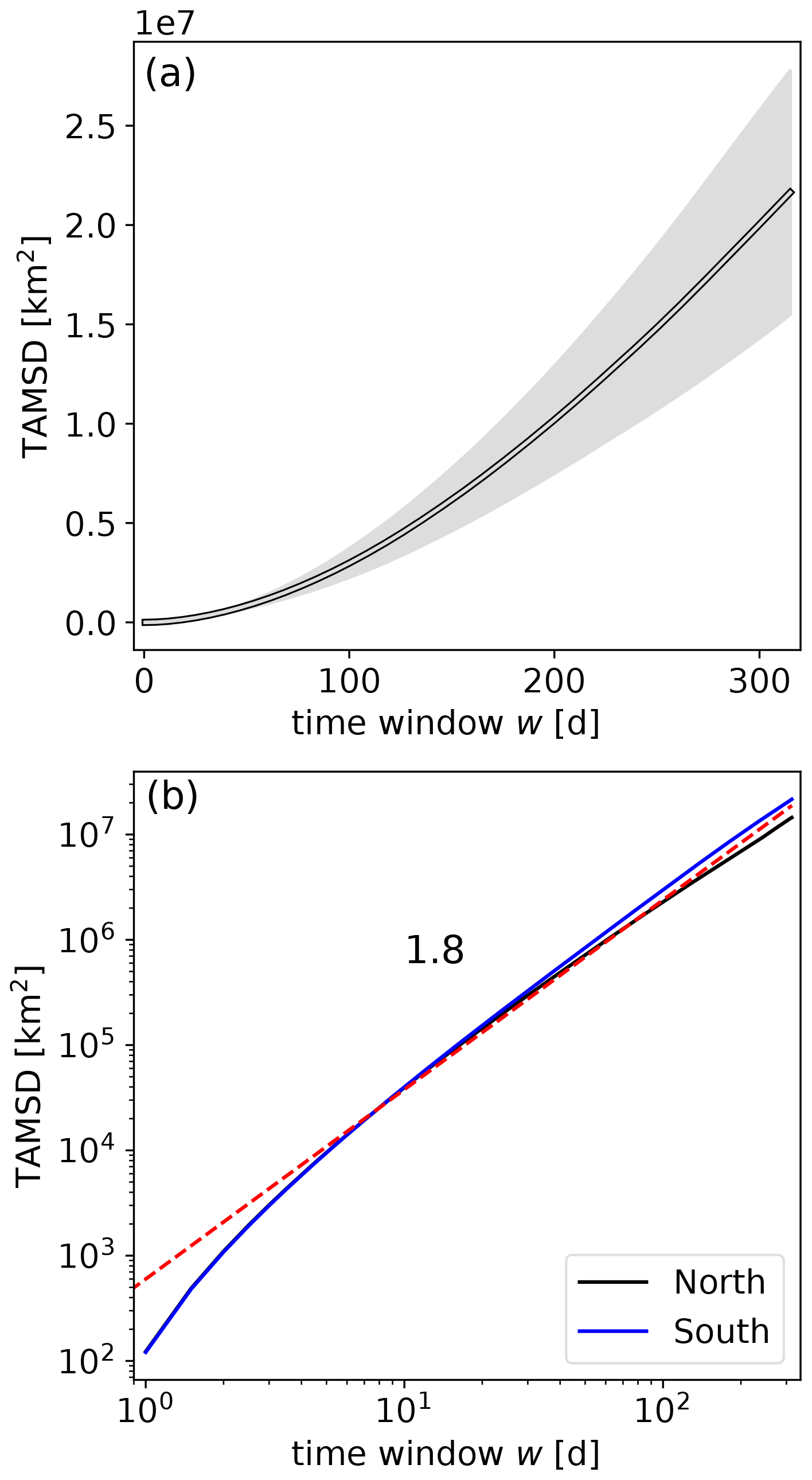
Figure 7 Time-averaged mean squared displacement (TAMSD) for the advected parcels in units of km². The spherical geometry was fully taken into account when calculating distances in moving time windows of size w. (a) TAMSD for the northern subset (lin-lin plot). The error band reflects the standard deviation obtained from year-by-year statistics. (b) TAMSDs for both the northern (black) and southern (blue) subsets of parcels on a double-logarithmic scale. The dashed red line illustrates a power law with an exponent value of around 1.8.

Firstly, we determine the mean squared displacement (MSD) as a function of time. The MSD is defined as the average over many trajectories (i.e., an ensemble average) of the square of the distance between the initial point and the endpoint at time t of each trajectory, so we use the formula

$$\begin{array}{}\text{(3)}& \mathrm{MSD}\left(t\right):=\langle \left(x\right(t)-x_{\mathrm{0}}{)}^{\mathrm{2}}\rangle ,\end{array}$$

where 〈…〉 denotes the average over all the trajectories with westward tendencies. For a classical diffusion process, it is known that MSD(t)∝t, while for ballistic motion (i.e., a purely deterministic drift), MSD(t)∝t². Empirically, we find that MSD(t)∝t^2H with H≈0.9 (see Fig. 6), i.e., faster than linear growth over time, but still less fast than ballistic motion. Such behavior is called superdiffusion (see, e.g., Bourgoin, 2015, and references therein), and in models it is caused by certain properties of the noise. For stationary increments, i.e., for a time-independent distribution of the noise, superdiffusion can be caused in two ways. The first is by long-range temporal correlations where the noise is not white but its autocorrelation function decays with the power law $c\left(\mathit{\tau }\right)\propto {\mathit{\tau }}^{-\mathrm{2}H-\mathrm{1}}$, and hence there is no finite correlation time. Alternatively, the noise can stem from a distribution with a fat tail, so it does not have a finite second moment. In this case, rare but huge jumps of the diffusive path allow particles to disperse much more quickly than they do diffusively. Any kind of superposition of these two mechanisms is also possible, so there are many different models that behave superdiffusively. We will employ additional analysis in order to identify the origin of this anomalous diffusive behavior.

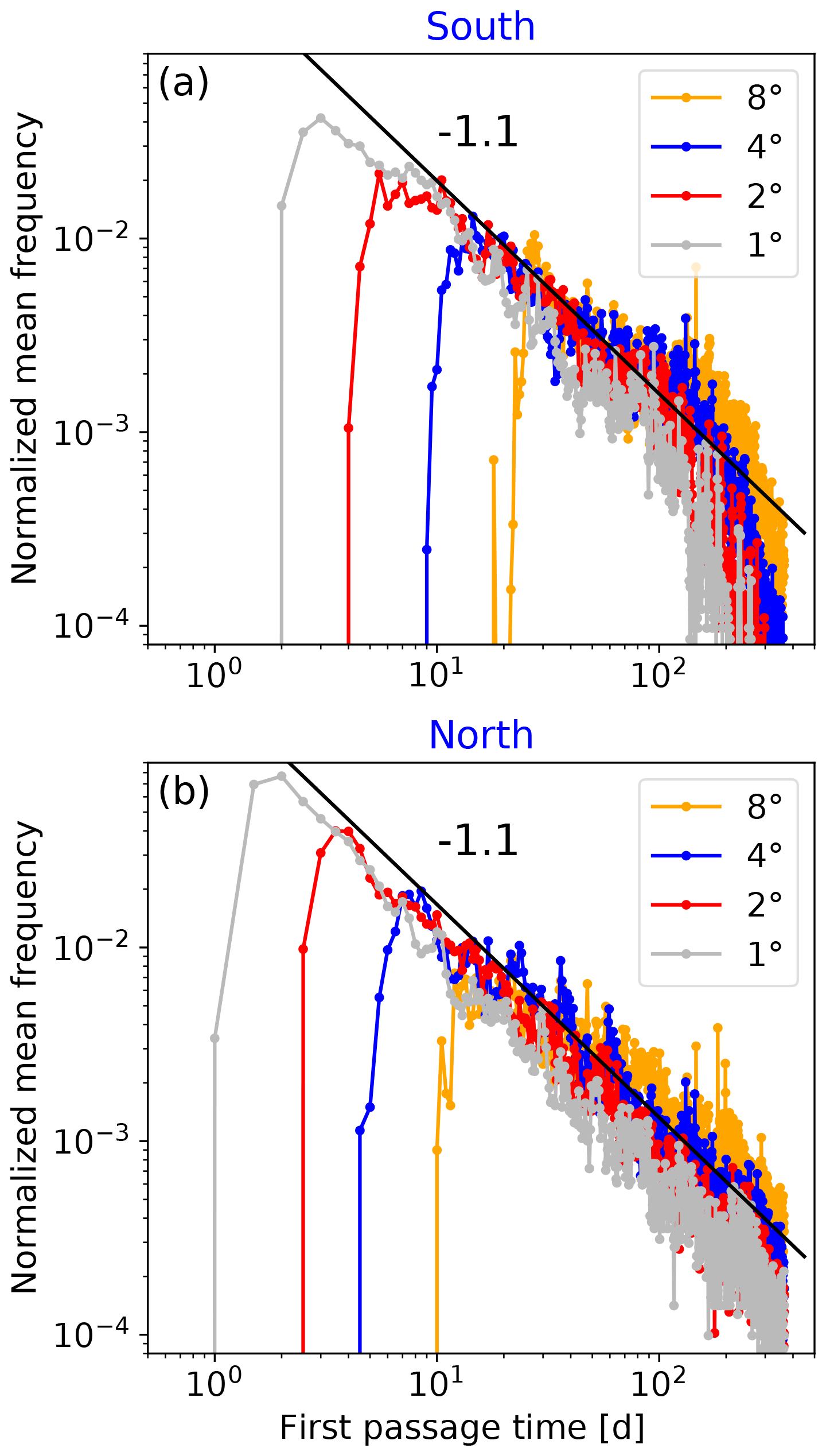
Figure 8 Normalized empirical frequency distribution of the first passage time (FPT) for the (a) southern subset and (b) northern subset of advected parcels on a double-logarithmic scale. Four different boundaries are shown at 1, 2, 4 and 8^∘ west from the initial positions of the tracers. The straight black line parallel to the envelopes illustrates a power law with an exponent value of around −1.1.

One such additional statistic is the time-averaged mean squared displacement TAMSD; see Fig. 7. Empirically, this displays power-law scaling with the same exponent ≈1.8 as the MSD. This is a signature of ergodicity (Metzler et al., 2014a), which restricts the choice of models further.

As a third statistic, we study the first passage time distribution. This is the distribution of the times needed by individual trajectories to pass through some predefined longitude circle. Since all particles start at 110^∘ W, this study considers the zonal motions of the tracers. We study four different positions of the line for passage, namely those that are 1, 2, 4 and 8^∘ west of the starting position. The corresponding distributions are shown in Fig. 8. The universal property of these distributions is a steep increase after some minimum time and a power-law decrease, t^−α. The power α (≈1.1) is independent of the line to be passed and is a further characteristic of the underlying stochastic process.

We evaluated the mean squared displacement of the particles up to distances of 10 000 km and for time windows of up to 1 year (Fig. 6), where the fractional Brownian motion model reproduces the observed anomalous diffusion well for the whole range of scales (see below). However, the nontrivial scaling of the MSD is not enough on its own to identify fractional Brownian motion as the correct model among several other anomalous diffusion processes, so we also performed a study of the first passage times. In this specific aspect, we restricted ourselves to distances and times of at most 900 km and 100 d, respectively. The reason for this is that, during many of the years (one is shown in Fig. 1a), a large fraction of the particles do not cross the 8^∘ distance from the place where they were released. This means that the number of particles that contribute to the first passage time distribution becomes smaller with increasing distance, and so, even for 16^∘, statistical sampling of the probability density is not good enough.

3.4 Fractional Brownian motion model

We can explain both behaviors of the tracers – that of the first passage time and that of the MSD – using a model of fractional Brownian motion (fBm). This is the path generated by accumulating (integrating) fractional Gaussian noise over time, and has two free parameters. One is the Hurst exponent H; the other is a generalized diffusion coefficient k_H, which determines the amplitude of the noise. For this model, it has been shown that the MSD scales as t^2H (Metzler and Klafter, 2000, 2004), i.e., the scaling of the MSD follows the same power law as the scaling of the TAMSD. The first passage time distribution shows a power law decay for large times, with power $\mathit{\alpha }=\mathrm{2}-H$ (Molchan, 1999). In addition, it is a Gaussian model, i.e., the distribution of the endpoints of trajectories as well as all distributions of the increments $x(t+\mathit{\delta })-x\left(t\right)$ are Gaussian for all t>0 and δ>0.

The results in Sect. 3.3 suggest that H=0.9. We can estimate the noise amplitude from the absolute values of the MSD in Fig. 6: the generalized diffusion coefficient is approximately 500 and 1000 km² d^−1.8 for the southern and northern parcels, respectively. Note that a direct comparison of the generalized diffusion coefficient k_H with those used in the literature for normal diffusion cannot be performed, since they have different units of time and roles in the model. In our superdiffusive fBm model, diffusion generates some effective drift. Compared to a model of normal Brownian diffusion plus an explicit ballistic drift, our model without an explicit drift term needs a larger generalized diffusion coefficient since it also generates an effective drift.

Let our time-discrete model of the time-continuous fractional Brownian motion have a time resolution of 1 d. Then the model noise amplitude is $\mathit{ϵ}=\sqrt{\mathrm{2}{k}_H}$. Hence, our model is $x\left(t\right)={\sum }_{i=\mathrm{1}}^t\mathit{ϵ}{\mathit{\xi }}_i$, where t is the time in days, ξ is the power-law-correlated Gaussian noise with unit variance and zero mean, and x(t) is the distance of the tracer from its starting position x(0)=0 in the zonal direction in km.

The results of the simulations are shown in Figs. 9 and 10. For the first passage time, we have approximated the distances from degrees using 111 km degree⁻¹, i.e., we numerically calculated the first passage time distributions for distances x of 111, 222, 444 and 888 km.

Sanders and Ambjörnsson (2012) suggest that the first passage time distribution has the following probability density:

$$\begin{array}{}\text{(4)}& \mathit{\varphi }\left(t\right)\simeq c{t}^{H-\mathrm{2}}\exp \left[-\mathit{\gamma }({\displaystyle \frac{s^{\mathrm{2}}}{\mathrm{4}{k}_H{t}^{\mathrm{2}H}}}{)}^{\mathit{\beta }}\right],\end{array}$$

where k_H is the abovementioned generalized diffusion coefficient, H is the Hurst exponent, which was estimated to be H≈0.9 for the ocean drifters, and the three free parameters c,βandγ are fitted to the process. Their values can only depend on H and k_H and the units of space and time, but they have not been derived analytically for the case of fractional Brownian motion, so we are free to fit them. Note, however, that they only affect the short-term behavior, since the exponential term tends to unity for large times t and the probability decays with the power law t^H−2.

Table 1 Fit parameters of the first passage time distribution (see Eq. (4)) to the empirical first passage times of the tracers in the northern (left) and southern (right) hemisphere. Notice that the essential parameter H has not been fitted but is given by the scaling of the MSD. Numerical fitting was performed by the nonlinear least squares method.

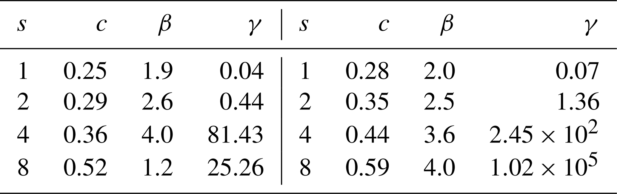
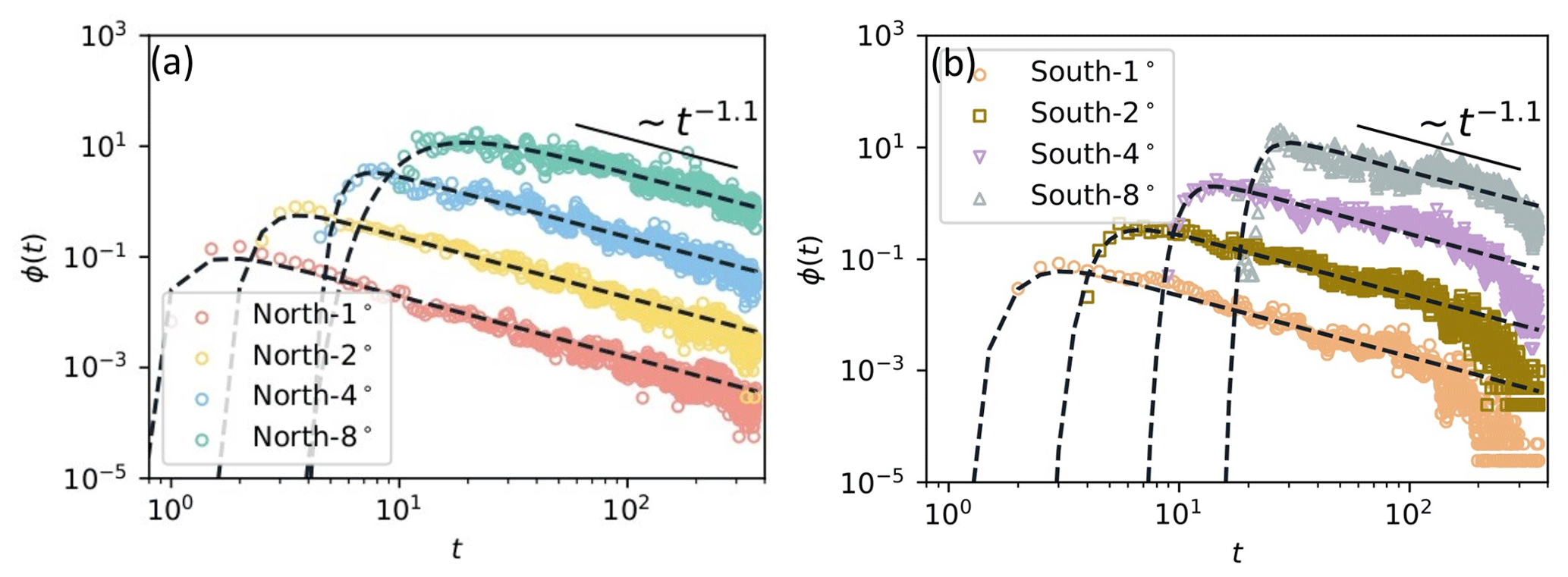
Figure 9 Comparison of the first passage time distribution of the fractional Brownian motion model (see Eq. (4)) with the empirical data for the (a) northern subset and (b) southern subset of advected parcels. Note that, to allow better visual comparison of the data to the fBm model, the values are multiplied by a factor of 10 for 2^∘, a factor of 100 for 4^∘ and a factor of 1000 for 8^∘.

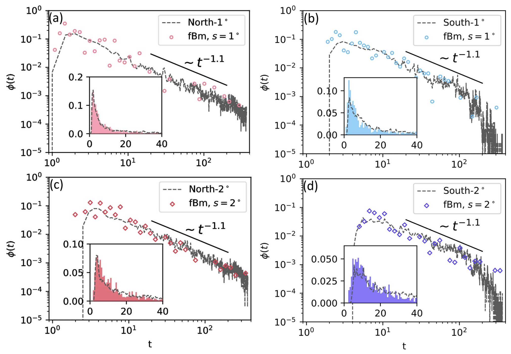
Figure 10 Comparison of the first passage time distribution of the fBm simulation with empirical data for the (a, c) northern subset (k_H=1000 km² d^−1.8) and (b, d) southern subset (k_H=500 km² d^−1.8) of advected parcels. The short solid black lines show the asymptotic behavior t^H−2 with Hurst exponent H=0.9, and the insets show the early behavior of the distribution on a linear scale. The time step Δt was chosen to be 0.0001 for 6600 runs.

We see in Fig. 9 that Eq. (4) with the parameters reported in Table 1 shows an excellent match to the empirical data from the oceanic tracers in the Northern and Southern hemispheres. Numerical simulations of this fractional Brownian motion process are in equally good agreement (Fig. 10), and we see that the fluctuations of the first passage time distribution of the oceanic tracer particles around the theoretical curve are of the same magnitude as the fluctuations of the numerical fBm trajectories, so they can be explained by mere statistical fluctuations.

In Fig. 1, we can see a quite clear westward drift for many of the trajectories. Such a drift term can also be included in the fractional Brownian motion model. A rough estimate of the drift velocity is about 5 km d⁻¹, so it is slow compared to the diffusion. While this slow drift leaves the bulk of the first passage time distribution unaffected, it might lead to a cutoff at long times. Such cutoffs can be seen in data from the Northern Hemisphere (see Fig. 10): after about 1 year, all tracers have reached the boundary, and the first passage time distribution drops to zero. Since this is a small correction, and since the development of the corresponding mathematical theory is still incomplete, we do not study here the fBm model with drift here.

While a pure fBm model has no preferred direction in space (i.e., particles diffuse both westward and eastward with the same statistics), reality suggests two modifications that can be included in our model: there are boundary conditions (the American continent) that prevent particles from moving eastward (this might be taken into account by including a reflecting boundary in our fBm model), and there might be a westward drift of a few km d⁻¹ that can be explicitly incorporated. Actually, the question of how much diffusion contributes to the westward advection is a very relevant one: our study tells us that if an explicit drift term is really needed in our model, it should be quite low – in the range of 5 km d⁻¹ or less. The strong persistence of the stochastic process, i.e., the long-range temporal correlations of the random increments to the path, ensures that steps change their signs rarely, and hence produce motion that looks as if it is being directed over long time intervals. Therefore, in the fBm model, the apparent drift is a sole consequence of the persistence of fBm, and we are able to reproduce the statistical properties of the tracers without including a drift term.

4 Conclusions

We have studied oceanic transport in the equatorial Pacific using observed and publicly available fields of surface velocities. Within these time-dependent fields, we numerically studied the trajectories of tracer particles released along a latitude circle at 110^∘ W within the latitude range [$-\mathrm{15}{}^{\circ }$,$+\mathrm{15}{}^{\circ }$]. We found nontrivial cross-correlations between advection indices and indices representing ENSO, with a time lag of 3 months. Beyond that, the erratic motions of individual particles showed two phenomena: an overall westward drift, which has been described in many previous articles, and the random deviations from this mean flow, which is in the focus of our world.

We should mention a possible limitation of the advection indices we defined. Since all the parcels start from the eastern boundary of the Pacific basin, the tracer cloud spreads gradually westward (mostly), and covers different regions after different time intervals throughout the year. In this respect, the eastern basin seems to dominate the statistics. Firstly, we emphasize that the statistical theories of random advection processes refer to the same situation: a cloud of tracers released from a restricted region that is gradually affected by the changing flow field with ever-increasing time. Secondly, we argue that, e.g., a uniformly distributed initial configuration (similar to drifting surface buoys at a given time instant) also has some shortcomings. Parcels starting from the western part of the basin quickly approach the coastal areas of the numerous islands and the continent; therefore, their trajectories are deflected by the local currents mostly in the meridional direction, and give a spurious contribution to the westward drift statistics. This is also the reason why we restricted an experiment to 1 year.

Using the statistics of the mean squared displacement , we found that the trajectory randomness is related to superdiffusion, i.e., the dispersion of particles is much faster than would be the case for a normal diffusion process (Figs. 6 and 7). This may be of high relevance to the spread of pollutants. A study of first passage times showed us that this process is well described by fractional Brownian motion. This implies that the statistics are still Gaussian, but the “noise” that makes the tracers diffuse has long-range temporal correlations. Indeed, long-range temporal correlations have been observed in many geophysical data sets before, such as in temperature and precipitation time series, but the Hurst exponent H≈0.9 is particularly large here, so the stochastic process is strongly non-Markovian and has a long memory.

We conclude that the collective effects of the spatial and temporal fluctuations of the velocity field that advects the particles have some self-similar structure that gives rise to a rather uniform time evolution on average over several years. In the end, our model contained only two parameters: the Hurst exponent H and the generalized diffusion coefficient k_H. This is a huge simplification compared to the simulation of the advection process, and will be useful for modeling and predicting the spread of advected passive scalars such as pollutants, nutrients or thermal energy in this region of the ocean.